Ada-XG-CatBoost: A Combined Forecasting Model for Gross Ecosystem Product (GEP) Prediction

Abstract

The degradation of the ecosystem and the loss of natural capital have seriously threatened the sustainable development of human society and economy. Currently, most research on Gross Ecosystem Product (GEP) is based on statistical modeling methods, which face challenges such as high modeling difficulty, high costs, and inaccurate quantitative methods. However, machine learning models are characterized by high efficiency, fewer parameters, and higher accuracy. Despite these advantages, their application in GEP research is not widespread, particularly in the area of combined machine learning models. This paper includes both a GEP combination model and an explanatory analysis model. This paper is the first to propose a combined GEP prediction model called Ada-XGBoost-CatBoost (Ada-XG-CatBoost), which integrates the Extreme Gradient Boosting (XGBoost), Categorical Boosting (CatBoost) algorithms, and SHapley Additive exPlanations (SHAP) model. This approach overcomes the limitations of single-model evaluations and aims to address the current issues of inaccurate and incomplete GEP assessments. It provides new guidance and methods for enhancing the value of ecosystem services and achieving regional sustainable development. Based on the actual ecological data of a national city, data preprocessing and feature correlation analysis are carried out using XGBoost and CatBoost algorithms, AdaGrad optimization algorithm, and the Bayesian hyperparameter optimization method. By selecting the 11 factors that predominantly influence GEP, training the model using these selected feature datasets, and optimizing the Bayesian parameters, the error gradient is then updated to adjust the weights, achieving a combination model that minimizes errors. This approach reduces the risk of overfitting in individual models and enhances the predictive accuracy and interpretability of the model. The results indicate that the mean squared error (MSE) of the Ada-XG-CatBoost model is reduced by 65% and 70% compared to the XGBoost and CatBoost, respectively. Additionally, the mean absolute error (MAE) is reduced by 4.1% and 42.6%, respectively. Overall, the Ada-XG-CatBoost combination model has a more accurate and stable predictive performance, providing a more accurate, efficient, and reliable reference for the sustainable development of the ecological industry.

1. Introduction

The degradation of ecosystems and the loss of natural resources have raised significant concerns about the reduction in ecosystem services, which pose serious threats to the sustainable development of human society and the economy [1]. Although the global economy, as measured by traditional Gross Domestic Product (GDP), more than doubled from 1990 to 2015, the reserves of global ecosystem assets—such as forests, grasslands, wetlands, soils, climate, and biodiversity—and the flow of ecosystem services they provide are under increasing pressure [2]. While GDP can quantify economic growth and development factors, it neglects the crucial contributions of natural resources to economic benefits [3]. In recent years, people have increasingly recognized the significant flaws in the way we measure development and well-being. More and more countries are placing emphasis on evaluating the value of ecosystem services to achieve a win–win scenario for ecological conservation and economic development [4,5].

These ecosystem services often have significant importance, but their value is frequently ignored or underestimated [6]. To achieve sustainable development, it is imperative to go beyond traditional economic indicators like GDP [7,8]. In response to this challenge, scholars have proposed the concept of Gross Ecosystem Product (GEP), which represents the total value of all final products and services provided by ecosystems for human well-being and sustainable economic and social development in a specific region [9]. The concept of GEP was initially proposed by the ecological economist Hannon [10]. Domestically, the concept of GEP was first introduced in 2013 by Ouyang et al. [11] when calculating the provincial-level GEP of Guizhou Province, and since then, numerous related studies have been conducted in China. The significance of GEP research lies in monetizing the value of ecosystem services, providing crucial support for policymakers to monitor changes in ecological values, achieve regional sustainable development, and promote the realization of ecosystem service values [12,13].

Currently, most GEP research focuses on ecologically representative regions [14,15,16], leading to incomplete assessments. Additionally, traditional statistical modeling is predominantly used [17,18,19,20], which presents significant challenges. Rao et al. [21] evaluated specific ecosystem types, including forests, wetlands, mountains, coasts, and lakes. These studies primarily have focused on individual ecosystem types and urbanized areas [22,23,24]. However, they lack a comprehensive assessment and accounting framework, failing to reflect the value of the entire ecosystem. Subsequent scholars have conducted extensive research at the global, national, and provincial levels [11,25,26,27,28,29], employing various research methods, including statistical analysis, market valuation, the water balance method, shadow engineering method, the replacement cost, the value transfer method, the travel cost method, and the hedonic pricing method to create corresponding models [12,30,31,32,33,34]. However, these methods are associated with significant challenges, such as high modeling complexity, high evaluation costs, and substantial time and effort requirements. Additionally, Costanza et al. [35] verified that among all the methods used, the value transfer method is more effective in estimating GEP [35,36]. However, the results from different studies can vary by more than 100 times [37].

With the widespread adoption of machine learning models, their high efficiency, minimal parameters, and high accuracy have prompted scholars both domestically and internationally to apply machine learning in GEP fields. He et al. [37] conducted a study on Potatso National Park using machine learning and big data analysis to evaluate the ecosystem service value of the national park. Wang et al. [38] used six machine learning models (MLP, RF, AdaBoost, GBDT, XGBoost, and LightGBM) to predict the gross primary productivity (GPP, an important component of GEP) of grasslands on the Mongolian Plateau, all of which achieved good results. The study also explored the main influencing factors and contribution rates of machine learning in GPP prediction. Yi et al. [39] used county-level administrative regions in China as samples and employed machine learning models to fit terrestrial ecosystems. Zhu et al. [40] developed three traditional machine learning (ML) models and a deep learning (DL) model using stacked autoencoders (SAEs) to estimate the grassland ecosystems in northern China. They focused on the alpine and temperate grasslands of northern China, achieving a prediction accuracy of 85%. Xiao et al. [41] developed an improved regression tree method to create a net ecosystem exchange (NEE) prediction model, which accurately predicted NEE. DPS et al. [42] tested four major plant functional types in North America and used support vector regression (SVR) and random forest (RF) to model the time series of GPP. They verified that machine learning models performed well in simulating GPP. Wang et al. [43] utilized machine learning algorithms to analyze the total ecosystem product of the Xilinhot grassland ecosystem.

According to the aforementioned literature review, traditional statistical modeling and current machine learning modeling methods face challenges in terms of accuracy and the assessment of ecological diversity. Additionally, they did not perform differentiated assessment analysis or comprehensive model evaluation, leading to significant inaccuracies in the results. The above literature has limited the scope of GEP research by focusing only on specific ecological types.

Therefore, this study employed XGBoost, CatBoost, and Ada-XG-CatBoost to conduct a comprehensive evaluation of 11 types of ecosystems nationwide. This approach significantly reflects the value of the entire ecosystem. Moreover, the three machine learning models proposed in this study show excellent results in predicting the value of the entire ecosystem. Notably, the newly introduced Ada-XG-CatBoost model achieved encouraging results in predicting GEP.

2. Materials and Methods

2.1. Experimental Data Source

This article adopted a real dataset on 346 cities in China. Among them, the area of land use and cultural service data were derived from the Statistical Yearbook and statistical surveys. Regulating service data are derived from the Statistical Yearbook and relevant departments. For the model, 80% of the sample points were selected as training data, and the remaining 20% of the sample points were used as test data.

Soil conservation, air purification, climate regulation, water conservation, oxygen release and carbon sequestration, evaporation, and other characteristics were the input features for the machine learning models. The specific parameters and the unit are shown in

Table 1. Specific parameters of ecosystem data and units.

Criterion	Ecological Indicators	Secondary Indicators	Units	Data Source
Provisioning Service	Agricultural products	Agricultural product value	Billions	Statistical surveys
	Forestry products	Forestry product value	Billions
	Fishery products	Fishery product value	Billions
	Livestock products	Livestock product value	Billions
Regulating Services	Water conservation	Evaporation	mm	Local meteorological bureau, water conservancy bureau, and related departments
		Precipitation
	Soil conservation	Soil conservation
	Flood water storage	Heavy rainfall	mm
	Oxygen release and carbon sequestration	Nitrogen fixation
	Climate regulation	High-temperature days	days
	Air purification	NO purification
		SO purification
		Dust purification
Cultural Services	Tourism income	Gross tourism income	Billions	Statistical Surveys

below.

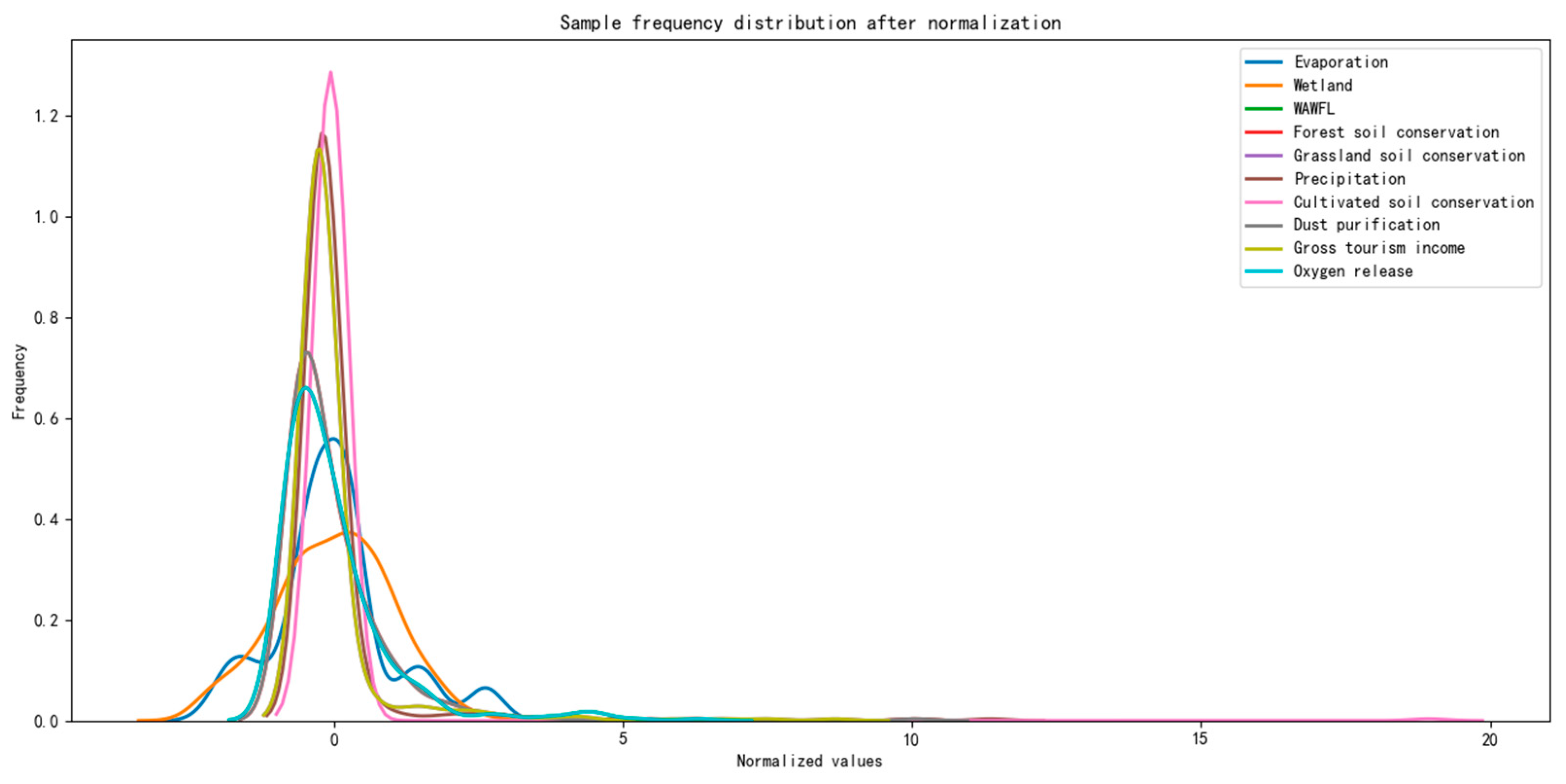
2.2. Data Preprocessing

Before training the model, the raw data needed to be preprocessed, including handling missing values, outliers, and normalization [44]. Common methods for dealing with outliers include deletion, treating outliers as missing values, mean correction, and capping. If outliers and missing values are not addressed, it can lead to a decline in model performance [45,46]. Considering that the experimental data came from real urban environments and has regional patterns, the interpolation method can better retain the data trends. Therefore, outliers can be treated as missing values and filled using interpolation based on the preceding and following data points in the feature space [47,48,49]. Common interpolation methods include Linear Interpolation, Polynomial Interpolation, Spline Interpolation, and Nearest Neighbor Interpolation [50]. Linear Interpolation is the simplest method, assuming linear change between two known data points, suitable for relatively smooth data variations. Polynomial Interpolation fits complex data changes but high-order polynomials can lead to overfitting, making it unsuitable for fitting GEP data. Spline Interpolation is ideal for smooth data variations [51]. However, GEP data are non-smooth and discrete. To more accurately fill in the missing values, we chose the Nearest Neighbor Interpolation method to handle anomalous data [52].

To prevent instability in prediction results due to infinite values and division by zero, we removed the heavy rainfall feature column, which had a large number of 0 values. Although there are also 0 and near-zero values in a very small number of other samples, considering the relatively small scale of the actual data, deleting these samples might impact the prediction results. Therefore, we retained these samples. [53].

To achieve improved model stability, convergence, and performance, as well as enhance the robustness of the model to input data and its generalizability across different scenarios [54], this article uses the Z-Score standardization method to convert the data to a distribution with a mean of 0 and a standard deviation of 1 and utilizes the StandardScaler class from the sklearn module to compute the mean and standard deviation of the feature columns in the data. This ensures that all the feature values adhere to a consistent scale following a normal distribution, which is beneficial for model training [55,56,57]. The standardization calculation formula is as follows (1):

$${\mathrm{X}}^{\prime }={\displaystyle \frac{\mathrm{X}-\mathsf{\mu }}{\mathsf{\delta }}}$$

(1)

In the formula, ${\mathrm{X}}^{\prime }$ is the sample data after the normalization process, $\mathrm{X}$ is the original sample data, $\mathsf{\mu }$ is a mean value characteristic, and $\mathsf{\delta }$ is the standard difference. The kernel density estimates for each feature were plotted using Seaborn’s kdeplot function, resulting in a normalized sample frequency distribution as shown in Figure 1 (only the normalized sample distribution of the candidate features is plotted in the figure).

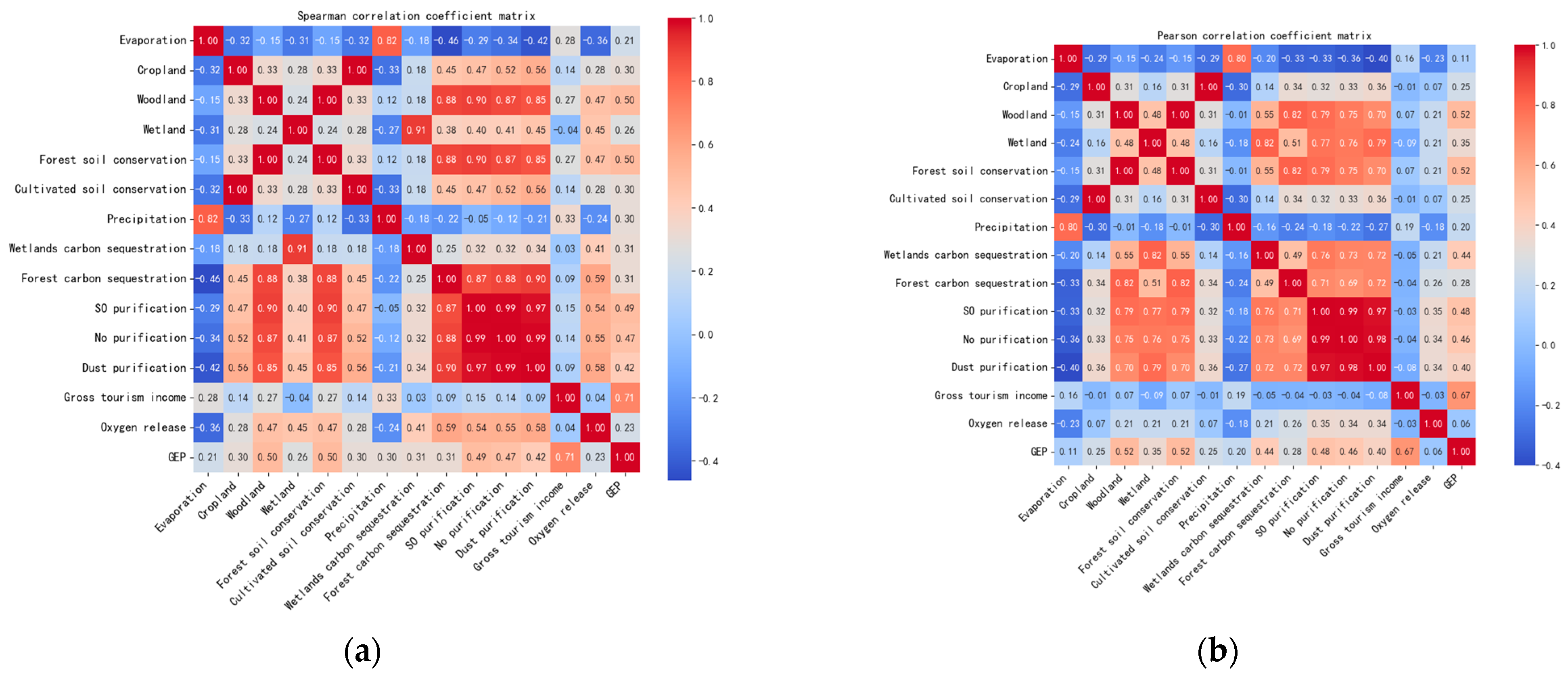
2.3. Feature Correlation Analysis

The authors of this article initially selected multiple explanatory variables, each affecting GEP differently. Some variables might have a low correlation with the final prediction results. Therefore, it was necessary to screen and analyze these 19 explanatory variables to improve the prediction accuracy of GEP. Pearson correlation coefficient is typically used to calculate the correlation between these 20 explanatory variables and GEP, as it measures the linear relationship between two variables. However, Pearson’s method assumes a linear relationship between variables and is not suitable when a strong but nonlinear relationship exists [58,59]. Given the complexity of the relationships between the explanatory variables and GEP, Pearson correlation may not be the most appropriate measure.

By calculating the Spearman rank correlation coefficient, we identified the correlations between the explanatory variables and the dependent variable [60]. The results show that 14 explanatory variables passed the two-tailed significance test at the 0.001 level. Spearman’s rank correlation coefficient is calculated using the following formula:

$$R_{rank}=1-{\displaystyle \frac{6{\sum }_{i=1}^n{D}^2}{n\left(n^2-1\right)}}$$

(2)

In the formula, $D$ represents the difference in ranks for each pair of data, and $n$ denotes the number of sample data points.

We utilized the Spearman rank correlation coefficient method to calculate the correlation coefficients between the 14 explanatory variables and GEP, and ranked these explanatory variables accordingly, as shown in Figure 2.

Among the initially selected explanatory variables, 14 variables passed the 0.01 two-tailed significance test, indicating a strong correlation with the dependent variable. Among them, gross tourism income has the highest correlation with GEP, with a coefficient of 0.71. This may be due to the differences in tourism expenditure levels across different regions, where regions with higher GEP may have higher tourism income.

This article presents a heatmap of the Spearman correlation coefficients (Figure 3), determined using a two-tailed test at the 0.001 significance level, to analyze the nonlinear strengths and directions of the relationships among the 14 explanatory variables [61].

There is evident multicollinearity among the initially selected 14 features. Therefore, it was necessary to use the Pearson correlation coefficient method to analyze the multicollinearity among these features. It can be seen that there is high multicollinearity between the NO purification, SO purification, and dust purification. Additionally, there is significant multicollinearity between the forest soil conservation and woodland, and between cropland and cultivated soil conservation [62,63,64].

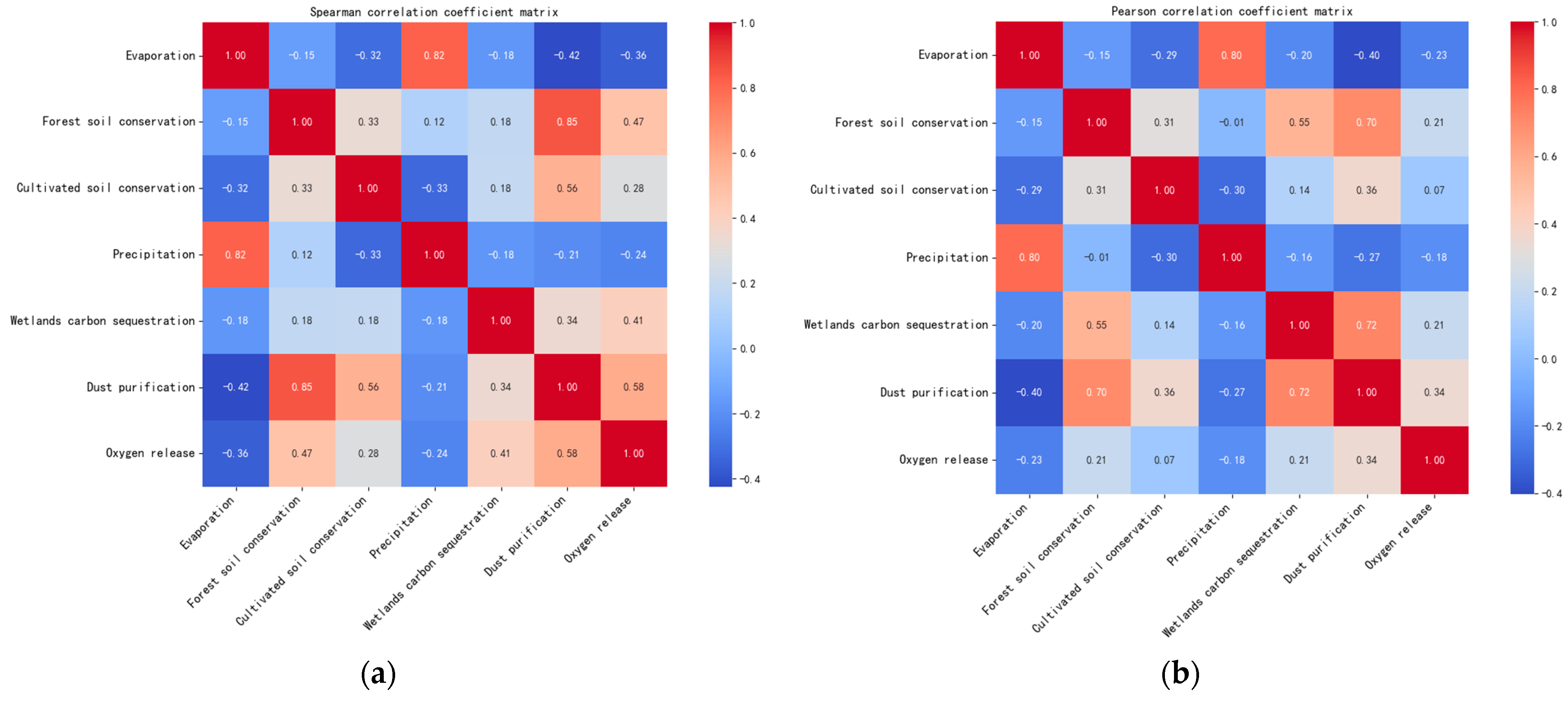
2.4. Feature Selection

After data preprocessing and feature correlation analysis, the candidate feature dataset is obtained. If the model is directly input for training, redundant noise and characteristic noise may be introduced, which will have a negative impact on the performance of the model and cause dimension disaster [65]. Especially for XGBoost, when there are many input features, the dimensions of the dataset will become large, which may cause problems such as insufficient memory and overfitting. The feature selection can conduct a quantitative analysis of the importance of features; delete the weak correlation features, which is lower than the setting threshold; reduce multiple correlations between features; reduce the model’s excessive risk; and improve the generalization of the model on the new data. Generally, an absolute correlation coefficient greater than 0.7 indicates a very close relationship; a coefficient between 0.4 and 0.7 suggests a strong relationship; and a coefficient of 0.1 or lower indicates a weak or negligible relationship [66,67,68].

To enhance the performance and efficiency of the model by selecting features that are highly correlated with the target variable yet non-redundant, this paper sets the threshold at 0.7. Since GEP is a complex issue, setting a threshold that is too low would result in discarding too many features, thereby failing to capture important information in the data. The final set of the extracted features totaled 7. The Pearson correlation matrix and Spearman rank correlation matrix heatmaps are shown in Figure 4. These 7 features were input into the machine learning model for training and testing.

2.5. Parameter Tuning

When using Python to train the training model, it is necessary to optimize the hyperparameters of the XGBoost and CatBoost models. Hyperparameter tuning methods include Grid Search, Random Search, Evolutionary Algorithms, and Bayesian optimization [69,70]. For models with extensive parameter spaces, Grid Search and Evolutionary Algorithms can be computationally expensive and inefficient. Random Search, while faster than Grid Search, does not guarantee finding the global optimal solution but can identify a good approximate solution. However, Bayesian optimization optimizes hyperparameters through a combination of model prediction and exploration, making it more efficient for searching parameter spaces [71,72].

In this paper, the bayesearchcv function was used to search the booster parameters, and the training samples were used to optimize the model parameters. The results of the booster parameter of XGBoost and CatBoost are shown in

Table 2. CatBoost hyperparameter settings.

Parameters	Hyperparameter Settings
depth	3
iterations	2000
learning rate	0.0099
subsample	0.6
colsample bytree	1.0
l2_leaf_reg	0.5

and

Table 3. XGBoost hyperparameter settings.

Parameters	Hyperparameter Settings
n_estimators	2000
max_depth	3
learning rate	0.027
subsample	1.0
Colsample bytree	1.0
reg_alpha	0.1
reg_lambda	1.0

.

2.6. Evaluation Indicator

Typically, R² (coefficient of determination), $MSE$ (mean squared error), $MAE$ (mean absolute error), and MAPE (mean absolute percentage error) are used as evaluation metrics to measure model performance. However, since MAPE is highly sensitive to zero values and cannot handle zero or very small values in the data samples, this could lead to calculation issues or biased results [73]. Therefore, we chose R², MAE, and MSE as the evaluation metrics to measure the performance of XGBoost, CatBoost, and Ada-XG-CatBoost. The definitions of the performance evaluation metrics used in this study are as follows:

$$R^2=1-{\displaystyle \frac{\sum \left(y_i-{\widehat{y}}_i\right){)}^2}{\sum (y_i-{\overline{y}}_i{)}^2}}$$

(3)

$$MAE={\displaystyle \frac{\sum \left|y_i-{\widehat{y}}_i\right|}{n}}$$

(4)

$$MSE={\displaystyle \frac{\sum {\left(y_i-{\widehat{y}}_i\right)}^2}{n}}$$

(5)

where $\widehat{y}$ indicates the prediction value of the target variable, $\overline{y}$ indicates the average value of the target variable, $\mathsf{\Sigma }$ represents the sum of the sum, and $i$ represents the number of samples.

2.7. Introduction to the Model

The models covered in this paper were all built in Python 3.11 using the Scikit-Learn 1.3.0, NumPy 1.26.2, and Pandas 2.1.1 libraries, and they were trained using an RTX 3050 Laptop GPU with 16 GB of memory.

For predicting GEP, commonly used machine learning algorithms include random forest (RF), Linear Regression, Neural Networks, Extreme Gradient Boosting (XGBoost), gradient boosting algorithm (CatBoost), and K-Nearest Neighbors (KNN) [74]. Different datasets are suitable for different algorithms. RF is suitable for handling large datasets and tends to perform better in such cases. KNN and Linear Regression are better suited for data with fewer outliers, and the relationship between the explanatory variables and GEP may not be entirely linear. Neural Networks can suffer from overfitting issues with smaller datasets. XGBoost and CatBoost are powerful gradient boosting algorithms known for their high predictive accuracy and their ability to prevent overfitting. They also maintain strong performance even in the presence of noise or outliers in the data [75].

Based on the above analysis, this study ultimately selected XGBoost and CatBoost as the final prediction models.

2.7.1. CatBoost

CatBoost stands for Gradient Boosting+Categorical Features, a GBDT framework based on a symmetric decision tree model, which has the advantages of supporting categorical variables, low hyper-parameter dependence, and high accuracy, and can effectively deal with categorical feature problems and reduce overfitting problems [76]. The advantages are as follows:

• Solves the problem of prediction bias: CatBoost uses a fully symmetric tree as a base model. It utilizes sort boosting to counteract anomalies in the dataset, which avoids the bias of gradient estimation and solves the problem of prediction bias.
• Effectively avoids overfitting: Leaf nodes are also calculated to select the structure of the tree when dealing with categorical features during the training process. CatBoost algorithm can deal with categorical features better on the basis of GBDT. CatBoost optimally upgrades the GBDT algorithm by adding a priori terms to reduce the influence of unfavorable factors such as noise and low-frequency data, as shown in Equation (6).

$${\widehat{x}}_k^{\left(i\right)}={\displaystyle \frac{\sum _{j=1}^{{\rm T}-1}\left[x_{\sigma j,k}=x_{\sigma {\rm T},k}\right]·Y_{\sigma j}+\alpha ·{\rm T}}{\sum _{j=1}^{{\rm T}-1}\left[x_{j,k}=x_{\sigma {\rm T},k}\right]+\alpha }}$$

(6)

where ${\rm T}$ is the a priori term and $\alpha$ is the weight of the a priori term ($\alpha$ > 0), the introduction of the a priori term helps to reduce the noise of the low-frequency category. In solving regression prediction problems, the a priori term $\alpha$ is usually taken as the mean of the dataset.

2.7.2. XGBoost

The Extreme Gradient Boosting Tree (XGBoost) model in ensemble learning algorithm boosting adds a regularization term to its cost function, which controls the complexity of the model and ensures the accuracy of the prediction results while avoiding the overfitting problem, which tends to give it an advantage [77].

The main idea of the XGBoost model is to generate the next learner based on the deviation between the result of the previous learner and the target, thus improving the model’s accuracy. The model uses several simple base learners and is very effective for studying regression problems. The superiority is shown below:

• High fitting accuracy: The XGBoost model utilizes a second-order Taylor’s formula to expand the loss function using both first-order and second-order derivatives as a way to improve the prediction accuracy.
• Lower model complexity: The XGBoost model adds regularization terms to the loss function of the gradient boosting decision tree (GBDT) to effectively reduce the model complexity. Its learning process is explained as follows:

$${\widehat{y}}_i=\sum _{i=1}^H{h}_k\left(x_i\right)$$

(7)

$$h_H\in \mathcal{B}$$

(8)

where $H$ is the number of trees; $h$ is a function in the function space $B$; ${\widehat{y}}_i$ is the model prediction; $x_i$ is the $i$th input data sample; and $\mathcal{B}$ is the set of all the possible CARTs. The prediction for step $t$ in the iterative process of the XGBoost algorithm is as follows:

$${\widehat{y}}_i=0$$

(9)

$${\widehat{y}}_i^{\left(1\right)}=h_1\left(x_i\right)={\widehat{y}}_i^{\left(0\right)}+h_1\left(x_i\right)$$

(10)

$${\widehat{y}}_i^{\left(2\right)}=h_1\left(x_i\right)+h_2\left(x_i\right)={\widehat{y}}_i^{\left(1\right)}+h_2\left(x_i\right)$$

(11)

$${\widehat{y}}_i^{\left(t\right)}=\sum _{k=1}^k{h}_k\left(x_i\right)={\widehat{y}}_i^{(t-1)}+h_i\left(x_i\right)$$

(12)

Therefore, the objective optimization function of the XGBoost algorithm is obtained as shown in Equation (13) as follows:

$$h_{obj}^{\left(t\right)}=\sum _{i=1}^{n}l(y_i,{\widehat{y}}_i^{\left(t\right)})+\sum _{i=1}^l\mathsf{\Omega }\left(h_i\right)=\sum _{i=1}^{n}l\left(y_i,{\widehat{y}}_i^{\left(t-1\right)}+h_t\left(x_i\right)\right)+\mathsf{\Omega }\left(h_i\right)+C$$

(13)

where $l$ is the loss function; $n$ is the number of observations; and Ω is the regularization term.

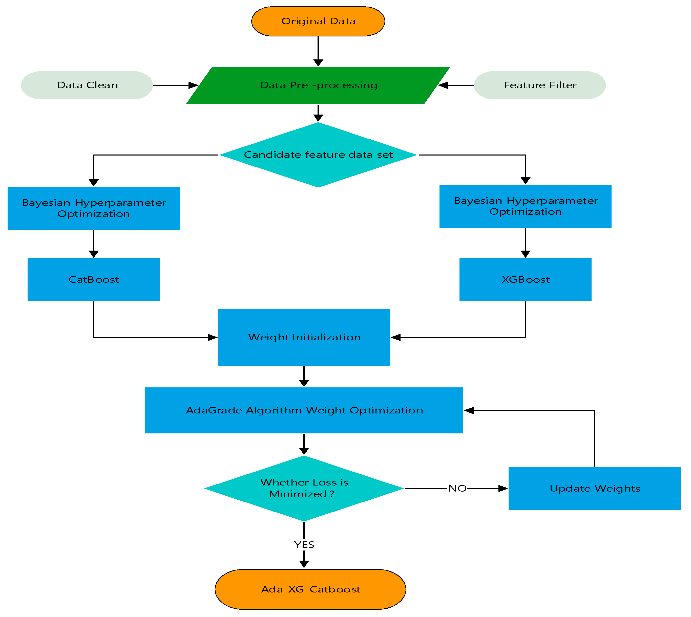
2.7.3. Ada-XGBoost-CatBoost

To overcome the limitations of a single model and improve the model’s ability to predict GEP [55,78,79], we used the Bayesian optimization algorithm to train and optimize the boost parameters of the individual models. Simultaneously, the AdaGrad optimization algorithm was utilized to optimize the weights of the Ada-XG-CatBoost ensemble, resulting in the prediction matrices of the trained individual models. The inverse error method is then used to assign greater weight to the individual models with better predictive performance. This approach ultimately yielded an ensemble model with the best predictive performance. Equation (14) represents the expression of the Ada-XG-CatBoost ensemble model:

$$y_{\mathrm{A}\mathrm{d}\mathrm{a}-\mathrm{X}\mathrm{G}-\mathrm{C}\mathrm{a}\mathrm{t}\mathrm{B}\mathrm{o}\mathrm{o}\mathrm{s}\mathrm{t}\_pred}=[\begin{array}{cc}w1& w2\end{array}][\begin{array}{c}{y}_{XGBoost\_pred}\\ y_{catboost\_pred}\end{array}]$$

(14)

$$w_1={\displaystyle \frac{MS{E}_{XGBoost}}{MS{E}_{CatBoost}+MS{E}_{XGBoost}}}$$

(15)

$$w_2={\displaystyle \frac{MS{E}_{CatBoost}}{MS{E}_{CatBoost}+MS{E}_{XGBoost}}}$$

(16)

where $w$₁ and $w$₂ are the initial weights of the gradient descent; $y_{XGBoost\_pred}$, $y_{catboost\_pred}$, and ${\mathrm{y}}_{\mathrm{A}\mathrm{d}\mathrm{a}-\mathrm{X}\mathrm{G}-\mathrm{C}\mathrm{a}\mathrm{t}\mathrm{B}\mathrm{o}\mathrm{o}\mathrm{s}\mathrm{t}\_pred}$ are the prediction results of the XGBoost, CatBoost, and XG-CatBoost combined models, respectively; and $MS{E}_{XGBoost}$ and $MS{E}_{CatBoost}$ are the mean squared error of XGBoost and CatBoost, respectively.

2.7.4. Combinatorial Modeling Strategies

The basic idea of combinatorial modeling is to combine the predictions of multiple models in different ways to achieve better overall performance while overcoming some of the limitations of a single model [80,81]. The common form of combinatorial predictive modeling is the weighted average of the individual predictive models, so the focus of combinatorial predictive modeling is on the determination of the weight values [82]. If the weighting coefficients of each single prediction model are assigned reasonable values, the prediction accuracy of the whole combination prediction model will be improved accordingly. In this study, we used the Bayesian hyperparameter search method to adjust the boosting parameters of XGBoost and CatBoost with the objective of minimizing the loss function. We used the AdaGrad optimization algorithm (Figure 5) to continually update the combined optimal weights of the two single models with a certain step size and train the models so as to improve the performance of the model and make the strengths and weaknesses of the single models complement each other.

3. Results and Discussion

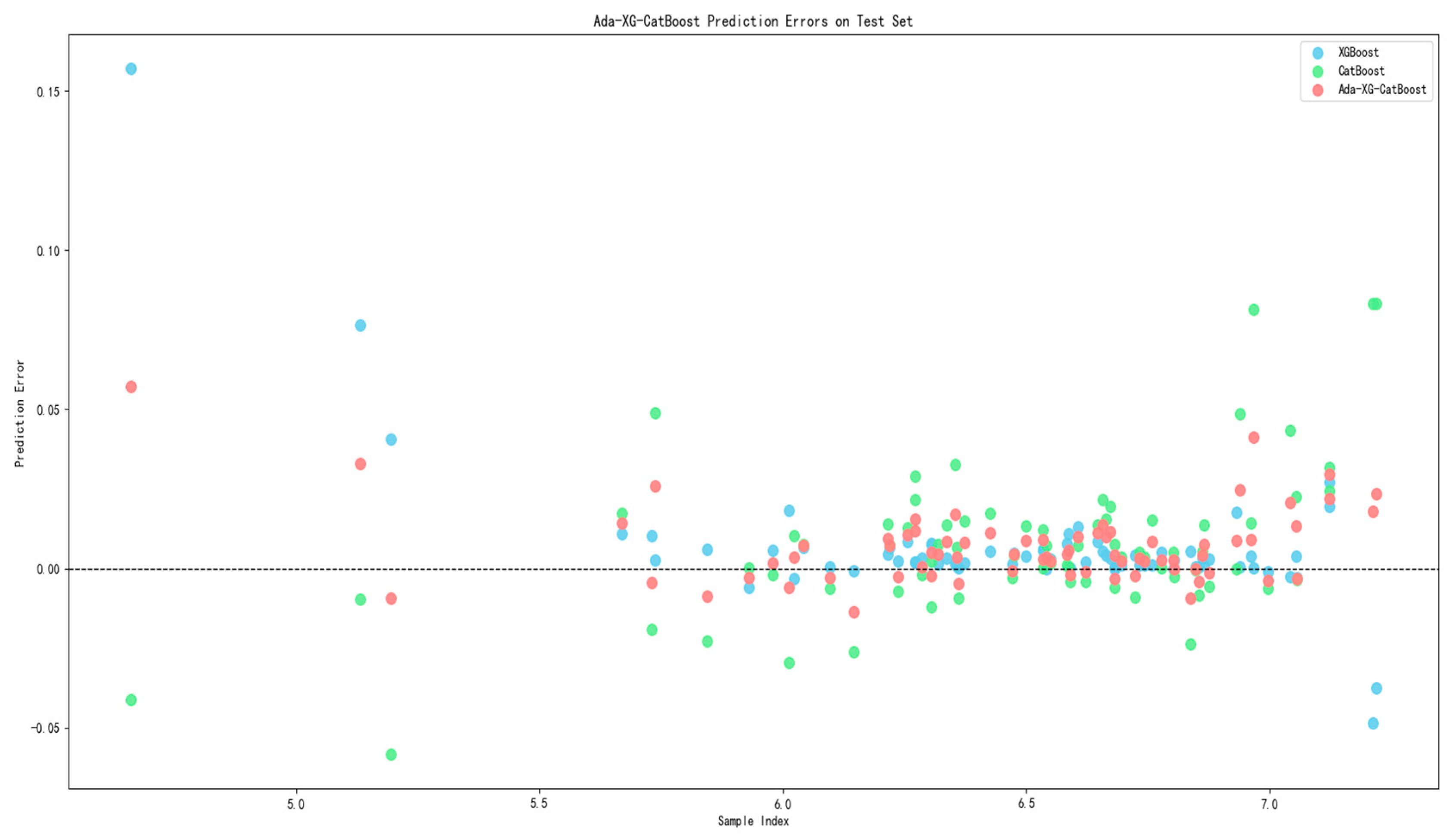
3.1. Models Performance Comparison and Analysis

To improve the performance of the XGBoost, CatBoost, and Ada-XG-CatBoost models on the test set, we conducted the following analysis:

Firstly, Bayesian hyperparameter optimization was employed to adjust the booster parameters of the XGBoost and CatBoost algorithms, yielding the optimal hyperparameter combinations. This ensured the effective training of the models for GEP prediction while avoiding overfitting. Secondly, the AdaGrad adaptive learning rate optimization algorithm was introduced. Combining the predictive performance of XGBoost and CatBoost, an early stopping strategy was adopted to monitor loss on the test set and analyze the models’ performance. Finally, based on the aforementioned methods, a model was constructed, and the Ada-XG-CatBoost model’s prediction results were obtained with the optimal weight matrix.

During the training of the Ada-XG-CatBoost model, the changes in weights w1 and w2 with the number of iterations are shown in Figure 6a, and the changes in the loss value with the number of iterations are shown in Figure 6b. As seen in Figure 6a, with the increase in iterations, the weights w1 and w2 of the Ada-XG-CatBoost model gradually converged after 250 iterations. Figure 6b shows that as the number of iterations increased, the loss value of the Ada-XG-CatBoost model during training also gradually stabilized, indicating that the Ada-XG-CatBoost model has found the optimal weights that minimized the loss.

When w1 = 0.50403207 and w2 = 0.49596793, the loss of the Ada-XG-CatBoost model was minimized, and the prediction accuracy reached its maximum value of 0.999.

The above indicators were used to evaluate the performance of the model. Different indicators can reflect the performance of the model in different aspects. The higher the R² is, the more accurate the prediction result is. The lower the MSE, RAE, and MAPE are, the more accurate the prediction results are.

Table 4. Evaluation results of XGBoost, CatBoost, and XG-CatBoost models.

	MSE	MAE	R2
XGBoost	0.00052	0.0097	0.9976
CatBoost	0.00060	0.0162	0.9973
Ada-XG-CatBoost	0.00018	0.0093	0.9992

presents the evaluation results for each model. The MSE (mean squared error) indicates prediction stability, with lower values representing more stable predictions. Based on the calculations, the Ada-XG-CatBoost model shows greater stability in predictions compared to the XGBoost and CatBoost models. The MSE values range from 0 to infinity, with values closer to 0 indicating better model performance. The MSE values for the models range from 0.0001 to 0.006, with the Ada-XG-CatBoost model achieving the lowest MSE. The CatBoost model’s MSE is slightly higher but still close. Additionally, all the performance metrics of the Ada-XG-CatBoost model are the best, making it suitable for predicting the national GEP.

Figure 7 displays the average predictions of the three trained models on the test dataset. Ada-XG-CatBoost exhibited the best performance (R² = 0.9992; MAE = 0.0093), followed by XGBoost (R² = 0.9976; MAE = 0.0097), and CatBoost (R² = 0.9973; MAE = 0.0162). When the frequency of the data samples was high, the scatter diagrams of the three models showed that they converged very closely on both sides of the reference line; that is, the prediction accuracy of the three models was high. It can be clearly seen in Figure 7 that compared to the other two single models, the overall prediction effect of the Ada-XG-CatBoost model was closer to the true value, and the predicted value was not too large or too small. It solved the problem of the prediction offset of a single model and overcame the limitations of a single model.

This indicates that the Ada-XG-CatBoost model can support national GEP prediction research.

The calculation results and errors of XGBoost, CatBoost, and Ada-XG-CatBoost on the test set are shown in Figure 8. Based on the comparative analysis of the errors in Figure 8, it is concluded that the errors of the three models on the test set are basically stable in the smaller range of [−0.08, 0.2], and the prediction errors of Ada-XG-CatBoost are more concentrated near the horizontal reference line compared to XGBoost and CatBoost. The predicted values of all three models are very close to the actual values, with the XG-CatBoost model exhibiting superior fitting performance and generalization ability.

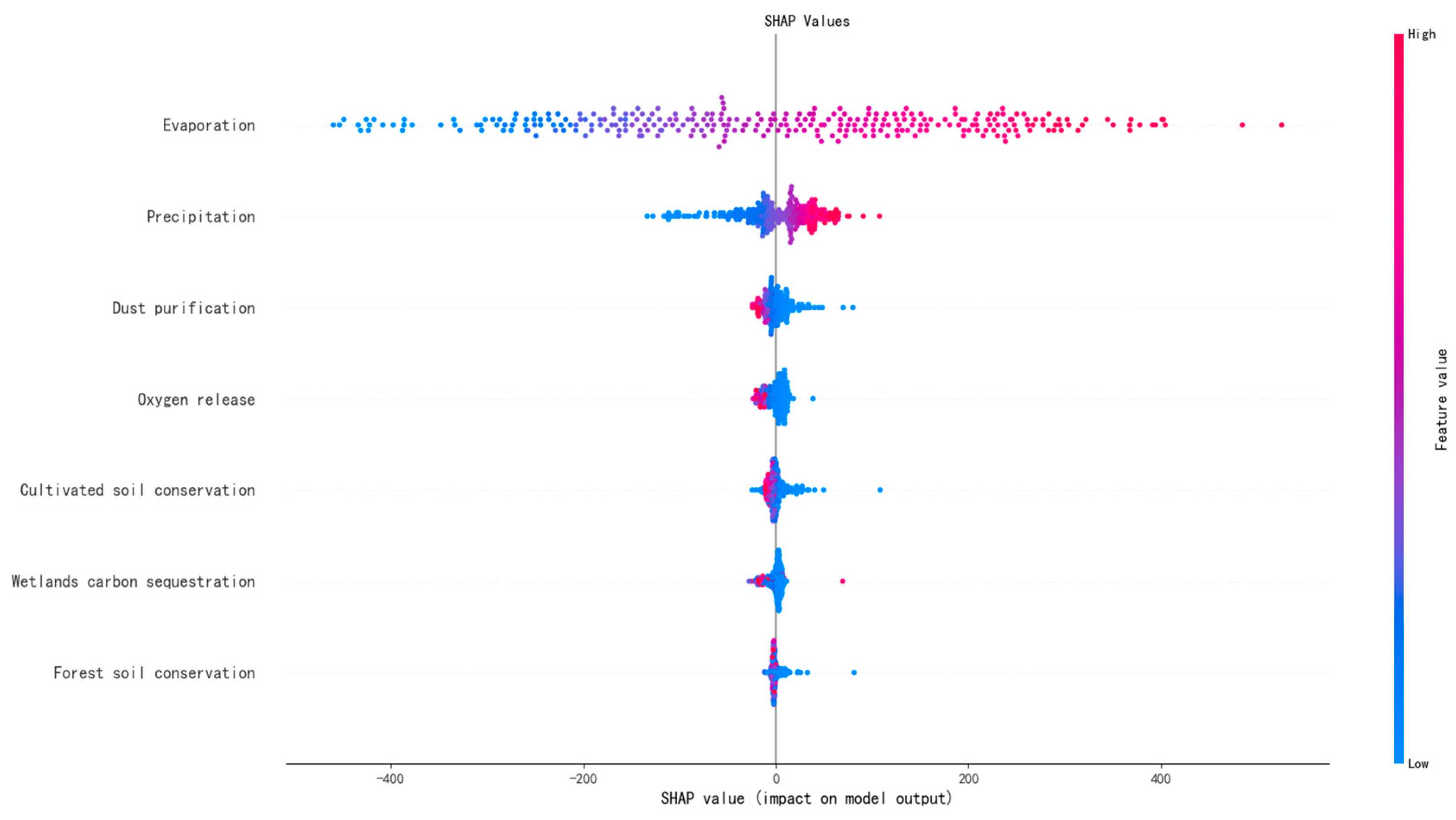
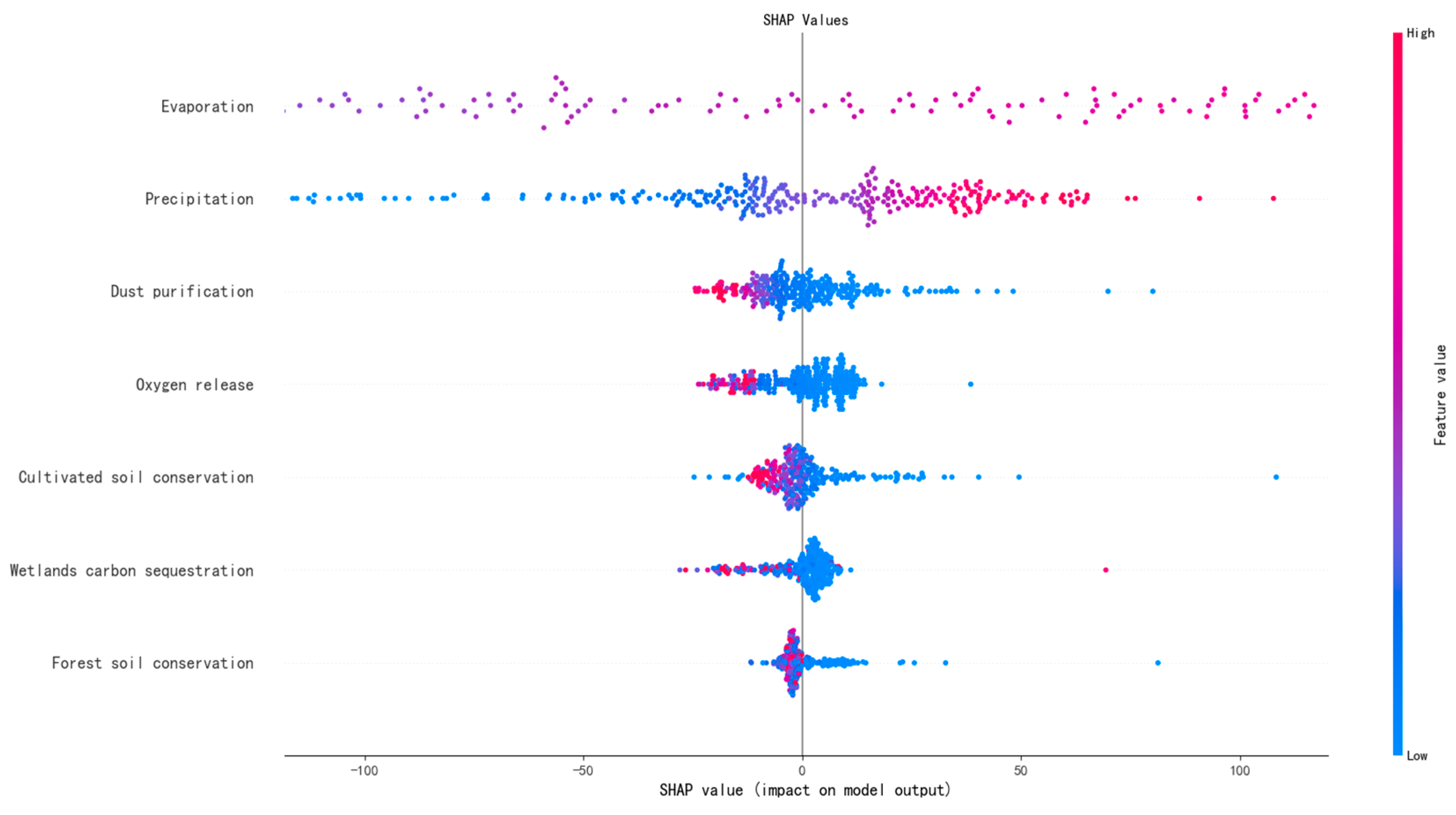
3.2. Model SHAP Value Interpretability Analysis

SHAP (Shapley Additive exPlanations) values are a method for interpreting machine learning model predictions using a fair and consistent method for assigning the degree to which each feature contributes to model predictions [83].

As shown in Figure 9, a SHAP plot was generated based on the weighted combination of XGBoost and CatBoost, illustrating the importance of the 11 influencing factors. This plot allowed for the interpretability analysis of the Ada-XG-CatBoost model, validating the importance of each feature to the model. In Figure 9, each dot represents a prediction sample, with the X-axis representing the SHAP values (the impact of the features on the output) and the Y-axis representing the influencing factors, indicating the extent to which each feature affects specific samples [84].

As shown in Figure 9, the feature of regional evaporation contributes the most to the GEP prediction. Secondly, the distribution of the blue and red points is relatively scattered, and the value range is large, which indicates that the influence of evaporation in different regions on the model prediction is different. Both the red and blue dots are more widely distributed, and the SHAP values of the red dots are both positive and negative, indicating that there is also not a simple linear relationship between the feature of evaporation and GEP; the areas with small amounts of evaporation have both positive and negative impacts on GEP prediction.

This indicates that different regional evaporation has different degrees of influence on the model predictions. Specifically, a negative SHAP value indicates a negative impact on GEP, a larger value of SHAP indicates a greater impact on GEP, and vice versa, i.e., the higher the regional evaporation, the higher the GEP and the greater the degree of impact on GEP, and vice versa. In addition, there are more red dots than blue dots, which reflects the country’s diverse climate and topography, as well as the predominance of inland areas. Since inland areas usually have arid or semi-arid climates, evaporation is relatively high in these areas, and thus, the magnitude of evaporation will show differences in different regions.

As shown in Figure 10, precipitation, dust purification, oxygen release, cultivated soil conservation, wetlands carbon sequestration, and forest soil conservation have varying degrees of influence on GEP. Specifically, the SHAP values for cultivated soil conservation and precipitation feature both positive and negative points, indicating a nonlinear relationship with GEP. When the SHAP value of precipitation is low, its effect on GEP prediction can be both positive and negative, meaning that regions with lower stormwater might have either high or low GEP.

Meanwhile, the SHAP values of precipitation, dust purification, oxygen release, cultivated soil conservation, wetlands carbon sequestration, and forest soil conservation have both positive and negative points, and larger SHAP values indicate a greater impact on GEP. However, the relationship is not simply linear, as both blue and red points in the figure have positive and negative values. The distributions of the blue and red dots also suggest a nonlinear relationship between these features and GEP. Specifically, when oxygen release, dust purification, wetlands carbon sequestration, and forest soil conservation are low, GEP distribution shows regularity. The blue and red points for the cultivated soil conservation are distributed in the negative value area of the SHAP plot. This indicates that, to some extent, increasing the value of cultivated land has a positive impact on GEP. However, once this value becomes too large, it may have a negative effect on GEP. For example, when the area of cultivated land increases, it can absorb and store large amounts of carbon, helping to mitigate climate change. However, an excessive increase in cultivated land area comes at the cost of natural habitats, leading to a decline in plant and animal species diversity. Additionally, too much cultivated land can result in decreased soil fertility and soil erosion, negatively impacting the soil’s carbon sequestration capacity. This can cause ecosystem instability and a reduction in biodiversity.

Overall, retaining the aforementioned influencing factors during feature selection is crucial for building an accurate GEP prediction model.

4. Conclusions

4.1. Research Content

In this study, we used a machine learning combinatorial modeling approach to predict GEP. This study utilized the PyCharm platform to evaluate the GEP of each city in China by using the Ada-XG-CatBoost combined model and developed the Ada-XG-CatBoost interpretable machine learning model. The aim of GEP planning research is to analyze and evaluate the contributions of ecosystems to human well-being, thereby accelerating the synergistic development of ecosystems and economic systems. This study draws the following conclusions:

• In terms of GEP prediction, the Ada-XG-CatBoost model is superior to the single models of XGBoost and CatBoost, with relatively high prediction accuracy and relatively good generalization ability. Compared to a single model, introducing a combined model enhances the mitigation of prediction bias, bolsters the model’s generalization performance and accuracy, and addresses the limitations of the individual models, resulting in more pronounced advantages.
• In practical GEP prediction studies, the Ada-XG-CatBoost combined model derived from the combination strategy serves as a more precise, efficient, and reliable generalization model. It offered a fresh approach and methodology for machine learning, offering significant reference value for government and local strategic planning.
• AdaGrad adaptively adjusted the learning rate based on the historical gradients of each parameter, eliminating the need for a globally fixed rate. The model achieved optimal weights after just 250 iterations, significantly reducing the iteration count and cutting down operational costs.
• This paper offered a novel research idea and model for GEP researchers. It not only simplifies the traditional statistical modeling of GEP but also enhances the accuracy of GEP assessment and valuation under high uncertainty. However, the study also faces some limitations [29,85].

4.2. Limitations for Future Work

This research seeks to establish practical methods to facilitate the conversion of resources, assets, and capital. However, there are still some limitations.

First, the Ada-XG-CatBoost model is not perfect. During data processing, in this study, we used the Nearest Neighbor Interpolation method to fill in the missing data values, which may reduce the performance of the model to some extent.

Second, we used Ada-XG-CatBoost and SHAP as interpretable machine learning methods to identify the main influencing factors, which may have overlooked a single model’s certain influencing factor. Future research can utilize methods like cross-validation to conduct multiple testing analyses on models, enhancing their generalizability and interpretability.

Finally, due to the limited dataset in this paper, we were not able to predict and evaluate GEP very accurately. In future research, we will consider adding multimodal information for further analyzing the feasibility of the model in GEP research, diversifying the data, and improving the model prediction performance.

In conclusion, the Chinese government attaches great importance to GEP and has conducted many pilot studies to promote its decision-making results.

References

1. Ma, G.; Yu, F.; Wang, J. Measuring gross ecosystem product (GEP) of 2015 terrestrial ecosystem in China. China Environ. Sci. 2017, 37, 1474–1482. [Google Scholar]
2. Ouyang, Z.; Song, C.; Zheng, H.; Polasky, S.; Xiao, Y.; Bateman, I.J.; Liu, J.; Ruckelshaus, M.; Shi, F.; Xiao, Y.; et al. Using gross ecosystem product (GEP) to value nature in decision making. Proc. Natl. Acad. Sci. USA 2020, 117, 14593–14601. [Google Scholar] [CrossRef] [PubMed]
3. Costanza, R.; de Groot, R.; Braat, L.; Kubiszewski, I.; Fioramonti, L.; Sutton, P.; Farber, S.; Grasso, M. Twenty years of ecosystem services: How far have we come and how far do we still need to go? Ecosyst. Serv. 2017, 28, 1–16. [Google Scholar] [CrossRef]
4. Jiang, W.; Wu, T.; Fu, B.J. The value of ecosystem services in China: A systematic review for twenty years. Ecosyst. Serv. 2021, 52, 101365. [Google Scholar] [CrossRef]
5. Aedasong, A.; Roongtawanreongsri, S.; Hajisamae, S.; James, D. Ecosystem services of a wetland in the politically unstable southernmost provinces of Thailand. Trop. Conserv. Sci. 2019, 12, 1940082919871827. [Google Scholar] [CrossRef]
6. Costanza, R.; de Groot, R.; Farber, S.; Grasso, M.; Hannon, B.; Limburg, K.; Naeem, S.; Paruelo, J.; Raskin, R.G.; Sutton, P.; et al. The value of the world’s ecosystem services and natural capital. Nature 1997, 387, 253–260. [Google Scholar] [CrossRef]
7. Xia, Q.-Q.; Chen, Y.-N.; Zhang, X.-Q.; Ding, J.-L. Spatiotemporal Changes in Ecological Quality and Its Associated Driving Factors in Central Asia. Remote Sens. 2022, 14, 3500. [Google Scholar] [CrossRef]
8. Nie, Z.; Li, N.; Pan, W.; Yang, Y.; Chen, W.; Hong, C. Quantitative Research on the Form of Traditional Villages Based on the Space Gene—A Case Study of Shibadong Village in Western Hunan, China. Sustainability 2022, 14, 8965. [Google Scholar] [CrossRef]
9. Ouyang, Z.; Zhu, C.; Yang, G.; Xu, W.; Zheng, H.; Zhang, Y.; Xiao, Y. Gross ecosystem product: Concept, accounting framework and case study. Acta Ecol. Sin. 2013, 33, 6747–6761. [Google Scholar] [CrossRef]
10. Bo, W.; Wang, L.; Cao, J.; Wang, X.; Xiao, Y.; Ouyang, Z. Valuation of China’s ecological assets in forests. Acta Ecol. Sin. 2017, 37, 4182–4190. [Google Scholar]
11. Cheng, M.; Huang, B.; Kong, L.; Ouyang, Z. Ecosystem Spatial Changes and Driving Forces in the Bohai Coastal Zone. Int. J. Environ. Res. Public Health 2019, 16, 536. [Google Scholar] [CrossRef] [PubMed]
12. Gowdy, J.; Howarth, R.; Tisdell, C. The Economics of Ecosystems and Biodiversity: Ecological and Economic Foundations; Rensselaer Polytechnic Institute: Troy, NY, USA, 2010. [Google Scholar]
13. Yu, M.; Jin, H.; Li, Q.; Yao, Y.; Zhang, Z. Gross Ecosystem Product (GEP) Accounting for Chenggong District. J. West China For. Sci. 2020, 49, 41–48. [Google Scholar]
14. Wang, P.; Chen, Y.; Liu, K.; Li, X.; Zhang, L.; Chen, L.; Shao, T.; Li, P.; Yang, G.; Wang, H.; et al. Coupling Coordination Relationship and Driving Force Analysis between Gross Ecosystem Product and Regional Economic System in the Qinling Mountains in China. Land 2024, 13, 234. [Google Scholar] [CrossRef]
15. Zhou, X.; Wang, Q.; Zhang, R.; Ren, B.; Wu, X.; Wu, Y.; Tang, J. A Spatiotemporal Analysis of Hainan Island’s 2010–2020 Gross Ecosystem Product Accounting. Sustainability 2022, 14, 15624. [Google Scholar] [CrossRef]
16. Li, Y.; Wang, H.; Liu, C.; Sun, J.; Ran, Q. Optimizing the Valuation and Implementation Path of the Gross Ecosystem Product: A Case Study of Tonglu County, Hangzhou City. Sustainability 2024, 16, 1408. [Google Scholar] [CrossRef]
17. Gao, J.; Yu, Z.; Wang, L.; Vejre, H. Suitability of regional development based on ecosystem service benefits and T losses: A case study of the Yangtze River Delta urban agglomeration China. Ecol. Indic. 2019, 107, 105579. [Google Scholar] [CrossRef]
18. Andersson, E.; Barthel, S.; Bergstrom, S.; Colding, J.; Elmqvist, T.; Folke, C. Reconnecting cities to the biosphere: Stewardship of green infrastructure and urban ecosystem services. MBIO 2014, 43, 445–453. [Google Scholar]
19. Liu, J.; Zhang, Q.; Wang, Q.; Liv, Y.; Tang, Y. Gross Ecosystem Product Accounting of a Globally Important Agricultural Heritage System: The Longxian Rice–Fish Symbiotic System. Sustainability 2023, 15, 10407. [Google Scholar] [CrossRef]
20. Boumans, R.; Roman, J.; Altman, I.; Kaufman, L. The Multiscale Integrated Model of Ecosystem Services (MIMES): Simulating the interactions of coupled human and natural systems. Ecosyst. Serv. 2015, 12, 30–41. [Google Scholar] [CrossRef]
21. Rao, N.; Ghermandi, A.; Portela, R.; Wang, X. Global values of coastal ecosystem services: A spatial economic analysis of shoreline protection values. Ecosyst. Serv. 2015, 11, 95–105. [Google Scholar] [CrossRef]
22. Sheng, L.; Jin, Y.; Huang, J. Value Estimation of Conserving Water and Soil of Ecosystem in China. J. Nat. Resour. 2010, 25, 1105–1113. [Google Scholar]
23. Bai, Y.; Li, H.; Wang, X.; Juha, M.A.; Jiang, B.; Wang, M.; Liu, W. Evaluating Natural Resource Assets and Gross Ecosystem Products Using Ecological Accounting System: A Case Study in Yunnan Province. J. Nat. Resour. 2017, 32, 1100–1112. [Google Scholar]
24. Xie, G.D.; Zhen, L.; Lu, C.X.; Xiao, Y.; Chen, C. Expert Knowledge Based Valuation Method of Ecosystem Services in China. J. Nat. Resour. 2008, 23, 911–919. [Google Scholar]
25. Liao, Z.; Zhou, B.; Zhu, J.; Jia, H. A critical review of methods, principles and progress for estimating the gross primary productivity of terrestrial ecosystems. Front. Environ. Sci. 2023, 11, 1093095. [Google Scholar] [CrossRef]
26. Qiu, X.; Zhao, R.; Chen, S. Review of Research on Value Realization of Ecological Products. China For. Prod. Ind. 2023, 6, 79–84. [Google Scholar]
27. Zou, Z.; Wu, T.; Xiao, Y.; Song, C.; Wang, K.; Ouyang, Z. Valuing natural capital amidst rapid urbanization: Assessing the gross ecosystem product (GEP) of China’s ‘Chang-Zhu-Tan’ megacity. Environ. Res. Lett. 2020, 15, 124019. [Google Scholar] [CrossRef]
28. Wang, W.; Xu, C.; Li, Y. Priority areas and benefits of ecosystem restoration in Beijing. Environ. Sci. Pollut. Res. Int. 2023, 30, 83600–83614. [Google Scholar] [CrossRef] [PubMed]
29. Zang, Z.; Zhang, Y.; Xi, X. Analysis of the Gross Ecosystem Product—Gross Domestic Product Synergistic States, Evolutionary Process, and Their Regional Contribution to the Chinese Mainland. Land 2022, 11, 732. [Google Scholar] [CrossRef]
30. Piyathilake, I.D.U.H.; Udayakumara, E.P.N.; Ranaweera, L.V.; Gunatilake, S.K. Modeling predictive assessment of carbon storage using invest model in Uva province, Sri Lanka. Model. Earth Syst. Environ. 2021, 8, 2213–2223. [Google Scholar] [CrossRef]
31. Ouyang, Z.; Lin, Y.; Song, C. Research on Gross Ecosystem Product (GEP): Case study of Lishui City, Zhejiang Province. Environ. Sustain. Dev. 2020, 45, 80–85. [Google Scholar]
32. Feng, M.; Liu, S.; Euliss, N.H., Jr.; Young, C.; Mushet, D.M. Prototyping an online wetland ecosystem services model using open model sharing standards. Environ. Model. Softw. 2011, 26, 458–468. [Google Scholar] [CrossRef]
33. Ondiek, R.A.; Kitaka, N.; Oduor, S.O. Assessment of provisioning and cultural ecosystem services in natural wetlands and rice fields in Kano floodplain. Kenya. Ecosyst. Serv. 2016, 21, 166–173. [Google Scholar] [CrossRef]
34. Wang, L.; Su, K.; Jiang, X.; Zhou, X.; Yu, Z.; Chen, Z.; Wei, C.; Zhang, Y.; Liao, Z. Measuring Gross Ecosystem Product (GEP) in Guangxi, China, from 2005 to 2020. Land 2022, 11, 1213. [Google Scholar] [CrossRef]
35. Costanza, R.; Groot, R.; Sutton, P.; van der Ploeg, S.; Anderson, S.J.; Kubiszewski, I.; Farber, S.; Turner, R.K. Changes in the global value of ecosystem services. Glob. Environ. Chang. 2014, 26, 152–158. [Google Scholar] [CrossRef]
36. Jiang, H.; Wu, W.; Wang, J.; Yang, W.; Gao, Y.; Duan, Y.; Ma, G.; Wu, C.; Shao, J. Mapping global value of terrestrial ecosystem services by countries. Ecosyst. Serv. 2021, 52, 101361. [Google Scholar] [CrossRef]
37. He, F.; Wei, X.; Zhou, J. Machine Learning-Driven Assessment of Ecological Resources: A Case Study in the Pudatso National Park. Yunnan Geogr. Environ. Res. 2023, 35, 1001–7852. [Google Scholar]
38. Wang, H.; Shao, W.; Hu, Y.; Cao, W.; Zhang, Y. Assessment of Six Machine Learning Methods for Predicting Gross Primary Productivity in Grassland. Remote Sens. 2023, 15, 3475. [Google Scholar] [CrossRef]
39. Yi, Z.; Wu, L. Identification of factors influencing net primary productivity of terrestrial ecosystems based on interpretable machine learning—Evidence from the county-level administrative districts in China. J. Environ. Manag. 2023, 326, 116798. [Google Scholar] [CrossRef]
40. Zhu, X.; He, H.; Ma, M.; Ren, X.; Zhang, L.; Zhang, F.; Li, Y.; Shi, P.; Chen, S.; Wang, Y.; et al. Estimating Ecosystem Respiration in the Grasslands of Northern China Using Machine Learning: Model Evaluation and Comparison. Sustainability 2020, 12, 2099. [Google Scholar] [CrossRef]
41. Xiao, J.F.; Zhuang, Q.L.; Baldocchi, D.D.; Law, B.E.; Richardson, A.D.; Chen, J.Q.; Oren, R.; Starr, G.; Noormets, A.; Ma, S.Y.; et al. Estimation of net ecosystem carbon exchange for the conterminous United States by combining MODIS and AmeriFlux data. Agric. For. Meteorol. 2008, 148, 1827–1847. [Google Scholar] [CrossRef]
42. Prakash Sarkar, D.; Shankar, U.; Parida, B.R. Machine learning approach to predict terrestrial gross primary productivity using topographical and remote sensing data. Ecol. Inform. 2022, 70, 101697. [Google Scholar] [CrossRef]
43. Wang, H.; Wu, N.; Han, G.; Li, W. Analysis of spatial-temporal variations of grassland gross ecosystem product based on machine learning algorithm and multi-source remote sensing data: A case study of Xilinhot, China. Glob. Ecol. Conserv. 2024, 51, 2942. [Google Scholar] [CrossRef]
44. Taamneh, M.M.; Taamneh, S.; Alomari, A.H.; Abuaddous, M. Analyzing the Effectiveness of Imbalanced Data Handling Techniques in Predicting Driver Phone Use. Sustainability 2023, 15, 10668. [Google Scholar] [CrossRef]
45. Amirivojdan, A.; Nasiri, A.; Zhou, S.; Zhao, Y.; Gan, H. ChickenSense: A Low-Cost Deep Learning-Based Solution for Poultry Feed Consumption Monitoring Using Sound Technology. AgriEngineering 2024, 6, 2115–2129. [Google Scholar] [CrossRef]
46. Liu, H.T.; Hu, D.W. Construction and Analysis of Machine Learning Based Transportation Carbon Emission Prediction Model. Environ. Sci. 2024, 45, 3421–3432. [Google Scholar]
47. Amir, A.; Henry, M. Reverse Engineering of Maintenance Budget Allocation Using Decision Tree Analysis for Data-Driven Highway Network Management. Sustainability 2023, 15, 10467. [Google Scholar] [CrossRef]
48. Bouguerra, H.; Tachi, S.E.; Bouchehed, H.; Gilja, G.; Aloui, N.; Hasnaoui, Y.; Aliche, A.; Benmamar, S.; Navarro-Pedreño, J. Integration of High-Accuracy Geospatial Data and Machine Learning Approaches for Soil Erosion Susceptibility Mapping in the Mediterranean Region: A Case Study of the Macta Basin, Algeria. Sustainability 2023, 15, 10388. [Google Scholar] [CrossRef]
49. Zhai, W.; Li, C.; Cheng, Q.; Ding, F.; Chen, Z. Exploring Multisource Feature Fusion and Stacking Ensemble Learning for Accurate Estimation of Maize Chlorophyll Content Using Unmanned Aerial Vehicle Remote Sensing. Remote Sens. 2023, 15, 3454. [Google Scholar] [CrossRef]
50. Alavi, S.H.; Bahrami, A.; Mashayekhi, M.; Zolfaghari, M. Optimizing Interpolation Methods and Point Distances for Accurate Earthquake Hazard Mapping. Buildings 2024, 14, 1823. [Google Scholar] [CrossRef]
51. Akbar, T.; Haq, S.; Arifeen, S.U.; Iqbal, A. Numerical Solution of Third-Order Rosenau–Hyman and Fornberg–Whitham Equations via B-Spline Interpolation Approach. Axioms 2024, 13, 501. [Google Scholar] [CrossRef]
52. Liu, R.; Gao, Z.-Y.; Li, H.-Y.; Liu, X.-J.; Lv, Q. Research on Molten Iron Quality Prediction Based on Machine Learning. Metals 2024, 14, 856. [Google Scholar] [CrossRef]
53. Song, W.; Feng, A.; Wang, G.; Zhang, Q.; Dai, W.; Wei, X.; Hu, Y.; Amankwah, S.O.Y.; Zhou, F.; Liu, Y. Bi-Objective Crop Mapping from Sentinel-2 Images Based on Multiple Deep Learning Networks. Remote Sens. 2023, 15, 3417. [Google Scholar] [CrossRef]
54. Hissou, H.; Benkirane, S.; Guezzaz, A.; Azrour, M.; Beni-Hssane, A. A Novel Machine Learning Approach for Solar Radiation Estimation. Sustainability 2023, 15, 10609. [Google Scholar] [CrossRef]
55. Wang, L.A. Study of China’s population forecast based on a combination model. Acad. J. Comput. Inf. Sci. 2022, 5, 76–81. [Google Scholar]
56. Zeng, J.; Dai, X.; Li, W.; Xu, J.; Li, W.; Liu, D. Quantifying the Impact and Importance of Natural, Economic, and Mining Activities on Environmental Quality Using the PIE-Engine Cloud Platform: A Case Study of Seven Typical Mining Cities in China. Sustainability 2024, 16, 1447. [Google Scholar] [CrossRef]
57. Zhu, H.; You, X.; Liu, S. Multiple Ant Colony Optimization Based on Pearson Correlation Coefficient. IEEE Access 2019, 7, 61628–61638. [Google Scholar] [CrossRef]
58. Saccenti, E.; Hendriks, M.H.W.B.; Smilde, A.K. Corruption of the Pearson correlation coefficient by measurement error and its estimation, bias, and correction under different error models. Sci. Rep. 2020, 10, 438. [Google Scholar] [CrossRef]
59. Ji, Y.; Zhang, Y.; Liu, D. Using machine learning to quantify drivers of aerosol pollution trend in China from 2015 to 2022. Appl. Geochem. 2023, 151, 105614. [Google Scholar] [CrossRef]
60. Muse, N.M.; Tayfur, G.; Safari, M.J.S. Meteorological Drought Assessment and Trend Analysis in Puntland Region of Somalia. Sustainability 2023, 15, 10652. [Google Scholar] [CrossRef]
61. Aviral Kumar, T.; Niyati, B.; Aasif, S. Stock Market Integration in Asian Countries: Evidence from Wavelet Multiple Correlations. J. Econ. Integr. 2013, 28, 441–456. [Google Scholar] [CrossRef]
62. Kim, G.Y.; Chung, D.B. Data-driven Wasserstein distributionally robust dual-sourcing inventory model under uncertain demand. Omega 2024, 127, 103112. [Google Scholar] [CrossRef]
63. Bian, L.H.; Ji, M.Q. Research on influencing factors and prediction of transportation carbon emissions in Qinghai. Ecol. Econ. 2019, 35, 35–39. [Google Scholar]
64. Mahjoub, S.; Labdai, S.; Chrifi-Alaoui, L.; Marhic, B.; Delahoche, L. Short-Term Occupancy Forecasting for a Smart Home Using Optimized Weight Updates Based on GA and PSO Algorithms for an LSTM Network. Energies 2023, 16, 1641. [Google Scholar] [CrossRef]
65. Skubleny, D.; Spratlin, J.; Ghosh, S.; Greiner, R.; Schiller, D.E. Individual Survival Distributions Generated by Multi-Task Logistic Regression Yield a New Perspective on Molecular and Clinical Prognostic Factors in Gastric Adenocarcinoma. Cancers 2024, 16, 786. [Google Scholar] [CrossRef]
66. Lukman, A.F.; Adewuyi, E.T.; Alqasem, O.A.; Arashi, M.; Ayinde, K. Enhanced Model Predictions through Principal Components and Average Least Squares-Centered Penalized Regression. Symmetry 2024, 16, 469. [Google Scholar] [CrossRef]
67. Sun, Z.; Wang, X.; Huang, H. Predicting compressive strength of fiber-reinforced coral aggregate concrete: Interpretable optimized XGBoost model and experimental validation. Structures 2024, 64, 106516. [Google Scholar] [CrossRef]
68. Chen, Y.; Yao, K.; Zhu, B.; Gao, Z.; Xu, J.; Li, Y.; Hu, Y.; Lin, F.; Zhang, X. Water Quality Inversion of a Typical Rural Small River in Southeastern China Based on UAV Multispectral Imagery: A Comparison of Multiple Machine Learning Algorithms. Water 2024, 16, 553. [Google Scholar] [CrossRef]
69. Tita, M.; Onutu, I.; Doicin, B. Prediction of Total Petroleum Hydrocarbons and Heavy Metals in Acid Tars Using Machine Learning. Appl. Sci. 2024, 14, 3382. [Google Scholar] [CrossRef]
70. Bobak, S.; Kevin, S.; Wang, Z. Taking the Human Out of the Loop: A Review of Bayesian Optimization. Proc. IEEE 2016, 104, 148–175. [Google Scholar]
71. Li, Y.; Abdallah, S. On hyperparameter optimization of machine learning algorithms: Theory and practice. Neurocomputing 2020, 415, 295–316. [Google Scholar] [CrossRef]
72. Storman, D.; Świerz, M.J.; Storman, M.; Jasińska, K.W.; Jemioło, P.; Bała, M.M. Psychological Interventions and Bariatric Surgery among People with Clinically Severe Obesity—A Systematic Review with Bayesian Meta-Analysis. Nutrients 2022, 14, 1592. [Google Scholar] [CrossRef] [PubMed]
73. Apostolos, A. Forecasting hotel demand uncertainty using time series Bayesian VAR models. Tour. Econ. 2018, 25, 734–756. [Google Scholar]
74. Osisanwo, F.; Akinsola, J.; Awodele, O.; Hinmikaiye, J.; Olakanmi, O. Supervised machine learning algorithms: Classification and comparison. Int. J. Comput. Trends Technol. 2017, 48, 128–138. [Google Scholar]
75. Praveena, M.; Jaiganesh, V. A literature review on supervised machine learning algorithms and boosting process. Int. J. Comput. Appl. 2017, 169, 32–35. [Google Scholar] [CrossRef]
76. Shao, Z.; Ahmad, M.N.; Javed, A. Comparison of Random Forest and XGBoost Classifiers Using Integrated Optical and SAR Features for Mapping Urban Impervious Surface. Remote Sens. 2024, 16, 665. [Google Scholar] [CrossRef]
77. Xiang, Q.; Wang, N.; Xiang, R. Prediction of Gas Concentration Based on LSTM-LightGBM Variable Weight Combination Model. Energies 2022, 15, 827. [Google Scholar] [CrossRef]
78. Xu, C.; Yi, W.; Biao, Z. Prediction of PM2.5 Concentration Based on the LSTM-TSLightGBM Variable Weight Combination Model. Atmosphere 2021, 12, 1211. [Google Scholar] [CrossRef]
79. Kim, Y.O.; Jeong, D.; Ko, I.H. Combining Rainfall-Runoff Model Outputs for Improving Ensemble Streamflow Prediction. J. Hydrol. Eng. 2006, 11, 578–588. [Google Scholar] [CrossRef]
80. Muhammad, A.; Stadnyk, T.A.; Unduche, F.; Coulibaly, P. Multi-Model Approaches for Improving Seasonal Ensemble Streamflow Prediction Scheme with Various Statistical Post-Processing Techniques in the Canadian Prairie Region. Water 2018, 10, 1604. [Google Scholar] [CrossRef]
81. Wang, X.; Wu, Z.; Wang, R.; Gao, X. UniproLcad: Accurate Identification of Antimicrobial Peptide by Fusing Multiple Pre-Trained Protein Language Models. Symmetry 2024, 16, 464. [Google Scholar] [CrossRef]
82. Mosso, D.; Rajteri, L.; Savoldi, L. Integration of Land Use Potential in Energy System Optimization Models at Regional Scale: The Pantelleria Island Case Study. Sustainability 2024, 16, 1644. [Google Scholar] [CrossRef]
83. Hjelkrem, L.O.; Lange, P.E.d. Explaining Deep Learning Models for Credit Scoring with SHAP: A Case Study Using Open Banking Data. J. Risk Financ. Manag. 2023, 16, 221. [Google Scholar] [CrossRef]
84. Airiken, M.; Li, S. The Dynamic Monitoring and Driving Forces Analysis of Ecological Environment Quality in the Tibetan Plateau Based on the Google Earth Engine. Remote Sens. 2024, 16, 682. [Google Scholar] [CrossRef]
85. Xie, H.; Li, Z.; Xu, Y. Study on the Coupling and Coordination Relationship between Gross Ecosystem Product (GEP) and Regional Economic System: A Case Study of Jiangxi Province. Land 2022, 11, 1540. [Google Scholar] [CrossRef]
Figure 1. Sample frequency distribution after normalization.
Sustainability 16 07203 g001
Figure 2. The correlation rankings of the 14 explanatory variables are shown.
Sustainability 16 07203 g002
Figure 3. Correlation heatmap with significance tested at the 0.001 level. (a) Spearman correlation coefficient matrix; (b) Pearson correlation coefficient matrix.
Sustainability 16 07203 g003
Figure 4. Heatmaps of correlation coefficient for candidate features. (a) Spearman correlation coefficient matrix; (b) Pearson correlation coefficient matrix.
Sustainability 16 07203 g004
Figure 5. Ada-XG-Catboost modeling flowchart.
Sustainability 16 07203 g005
Figure 6. Ada-XG-CatBoost model weights w1 and w2 and loss curves. (a) Ada-XG-Catboost model weight change curve. (b) Ada-XG-CatBoost test set loss iteration curve.
Sustainability 16 07203 g006
Figure 7. The fitting curves of the actual and predicted values for the XGBoost, CatBoost, and Ada-XG-CatBoost models on the test set.
Sustainability 16 07203 g007
Figure 8. Distribution of model predicted and true value residuals.
Sustainability 16 07203 g008
Figure 9. SHAP value of Ada-XG-CatBoost.
Sustainability 16 07203 g009
Figure 10. Localized enlargement of the SHAP value of Ada-XG-CatBoost.
Sustainability 16 07203 g010