Analysis of Wheat-Yield Prediction Using Machine Learning Models under Climate Change Scenarios

Abstract

Climate change has emerged as one of the most significant challenges in modern agriculture, with potential implications for global food security. The impact of changing climatic conditions on crop yield, particularly for staple crops like wheat, has raised concerns about future food production. By integrating historical climate data, GCM (CMIP3) projections, and wheat-yield records, our analysis aims to provide significant insights into how climate change may affect wheat output. This research uses advanced machine learning models to explore the intricate relationship between climate change and wheat-yield prediction. Machine learning models used include multiple linear regression (MLR), boosted tree, random forest, ensemble models, and several types of ANNs: ANN (multi-layer perceptron), ANN (probabilistic neural network), ANN (generalized feed-forward), and ANN (linear regression). The model was evaluated and validated against yield and weather data from three Punjab, Pakistan, regions (1991–2021). The calibrated yield response model used downscaled global climate model (GCM) outputs for the SRA2, B1, and A1B average collective CO₂ emissions scenarios to anticipate yield changes through 2052. Results showed that maximum temperature (R = 0.116) was the primary climate factor affecting wheat yield in Punjab, preceding the $T_{min}$ (R = 0.114), while rainfall had a negligible impact (R = 0.000). The ensemble model (R = 0.988, nRMSE= 8.0%, MAE = 0.090) demonstrated outstanding yield performance, outperforming Random Forest Regression (R = 0.909, nRMSE = 18%, MAE = 0.182), ANN(MLP) (R = 0.902, MAE = 0.238, nRMSE = 17.0%), and boosting tree (R = 0.902, nRMSE = 20%, MAE = 0.198). ANN(PNN) performed inadequately. The ensemble model and RF showed better yield results with $R^2$ = 0.953, 0.791. The expected yield is 5.5% lower than the greatest average yield reported at the site in 2052. The study predicts that site-specific wheat output will experience a significant loss due to climate change. This decrease, which is anticipated to be 5.5% lower than the highest yield ever recorded, points to a potential future loss in wheat output that might worsen food insecurity. Additionally, our findings highlighted that ensemble approaches leveraging multiple model strengths could offer more accurate and reliable predictions under varying climate scenarios. This suggests a significant potential for integrating machine learning in developing climate-resilient agricultural practices, paving the way for future sustainable food security solutions.

1. Introduction

Accurate wheat-yield projections are critical for sustaining agricultural practices and reducing the negative effects of climate change. Unlike prior studies, which mostly use traditional statistical methods, our research incorporates powerful machine learning algorithms to forecast wheat yield under various climate change scenarios [1]. Wheat is a vital cereal grain source, providing food for approximately 40% of the world’s population [2,3]. Most farmers, particularly those in developing nations, depend exclusively on their limited knowledge and prior experience. This limited knowledge makes it challenging for them to compete globally and fulfill expanding demands [4]. This study employs cutting-edge tools to investigate the complex interaction between climate conditions and wheat yield, providing more precise and useful findings.

Extreme weather, changing trends of rainfall, and rising temperatures are all things that could hurt food security and agriculture production. Uncertainty about the weather makes it hard to predict wheat yields, which are very important. Things like frost during the flowering and grain-filling stages, temperatures above 30 °C, and not enough rain at key times can all lead to production losses [5]. These problems already exist, and climate change will only make them worse. This will make it harder to plan and handle crops well.

The climate, management techniques, and personal standards can all affect the growth of a crop. Researchers use process-based and statistical methods, such as biological data and remote sensing [6,7,8], to keep an eye on production. Process-based models can be used for certain crops, like rice, wheat, and corn, to help with resource management and agriculture growth [9]. These models use correct data and algorithms to give farmers information that helps them make smart decisions. Statistical methods can also predict results in a wide range of situations by looking at how weather and land quality are linked to crops. Classical statistical methods based on mathematical models are often used to test ideas with crop samples. Their success, however, depends on having easy access to relevant farming data [10].

Global climate models (GCMs) are mostly used to guess how much food will be grown around the world in different weather and management situations. The best way to find out how climate change will affect crop growth is to use a GCM. GCMs have been used to model weather, land, management, and other aspects of agricultural development in order to predict food growth and output on a global and regional level. Different parts of the world have different weather, land, and ways of growing. Peng (2023) says that GCMs usually have a spatial resolution of 50 km × 50 km, which is good enough to obtain a good idea of national farming results. By adding these area factors, downscaling makes it possible to make more accurate and reliable estimates of crop yields. As Zhang (2019) says, the Coupled Model Intercomparison Phase 3 (CMIP3) collects GCM data from various sources to look into trends of climate change now and in the future. Using crop models and high-resolution climate data together, machine learning-based downscaling helps look at how climate change affects farming in specific areas. This study gives us useful information about how to change.

It is important to keep an eye on weather conditions like air temperature, CO₂, rainfall, and growing times when you are trying to adapt to a changing climate. Many studies have been conducted around the world to look at how climate change affects the output of crops. To show how climate change affects crop yields, Reference [11] used techniques for increasing yields that were part of the CMIP5 plan. As for Ishaque et al. [12], one way Pakistan might be able to change would be to move the best times to plant wheat to cooler months.

Using machine learning to fix problems has shown a lot of promise [13,14]. They are able to work with data that have a lot of dimensions, find relationships that are not straight, and see complex trends [15]. ML algorithms find links between dependent and independent factors by training them through spatiotemporal observational training on very large datasets. Machine learning techniques have been used in a number of ways to identify crops and predict their yields.

ML algorithms help with planning and running farms, and they are often used to guess how much food crops will produce. Models like artificial neural networks (ANNs), multiple linear regression (MLR) [16], random forest regression (RFR) [13,17], and XGboost [18] are used to estimate yields. These models consider things like temperature, humidity, wind speed, rainfall, and atmospheric gases. Overfitting is a problem with these models, which makes them less useful even when they do a good job of dealing with climate-related problems in agriculture. Using ensemble methods with multiple models makes yield predicting more accurate while reducing overfitting [19,20]. Ensemble methods, such as meta-machine learning, may improve the accuracy of wheat growth predictions by combining the results of many models.

When it comes to predicting climate change, statistical models and old methods that are based on past data often fall short. We suggest that this gap be filled by teaching a machine-learning model to predict wheat yields even when weather trends change. Machine learning algorithms may use enormous datasets to learn complicated correlations between variables and produce accurate predictions. The proposed solution integrates weather station data and CO₂ future emission scenarios to develop a precise machine-learning model capable of forecasting wheat yields. By accounting for climate change impacts on crop yields, our model empowers farmers to adapt their practices. The expected outcome is improved prediction accuracy, enhancing wheat production and food security. Similar studies using analogous methodologies have been conducted in other countries for different crops [21]. However, they did not use ensemble models, exposing a gap our research seeks to remedy. Our research stands out by combining ensemble modeling techniques, which aim to increase the robustness and accuracy of crop-yield projections.

Several studies have focused on forecasting crop production, especially in Pakistan, utilizing various predictors like rainfall, fertilizer, temperature, tractors, and labor. Previous research has highlighted the significant correlation between fertilizer application, remote sensing techniques, and wheat output [22,23,24,25].

More comprehensive studies that integrate multiple machine learning models specifically for wheat-yield prediction under climate change scenarios need to be conducted. While individual models have been explored, ensemble techniques that incorporate the advantages of many algorithms are required to improve forecast accuracy. Unlike previous studies that primarily relied on traditional statistical methods or focused on other regions [26], this work presents a novel way to predict wheat yield under climate change scenarios that employs a complex ensemble of machine learning models. The fundamental novelty of this research is the integration of many advanced machine learning algorithms to estimate wheat output based on climate data, which involves utilizing historical climate data as well as projections from GCMs. our research uniquely combines historical climate data, global climate model (GCM) projections, and advanced machine learning techniques. By doing so, we provide a comprehensive and accurate forecast of wheat yields specifically for Punjab, Pakistan. Our interdisciplinary approach advances agricultural yield prediction and offers practical insights for developing climate-resilient farming practices. These studies aim to enhance crop-forecasting accuracy by analyzing different factors’ effects on agriculture productivity, especially wheat production in Pakistan.

The key objective of this study is to construct a model for forecasting wheat yields via ANNs using meteorological and GCM data. To achieve this goal, the following tasks have been formulated:

• Identifying the key factors influencing wheat production
• Modeling and testing wheat-yield responses to rainfall and temperature variables using various methods such as boosting tree, ANNs, random forest regression, multiple linear regression, and ensemble models, based on observed yield and climatic data
• Anticipating and analyzing the potential influence of climate change on wheat crop trends up to the year 2052.

2. Materials and Methods

Certain materials and methods were used to conduct our experiments and analyze the data. We employed a novel combination of machine learning models to predict wheat yield. We carefully integrated random forest regression, boosted tree regression, artificial neural networks, and an ensemble model. Additionally, we preprocessed climate and yield data and applied advanced downscaling techniques to enhance the accuracy of localized prediction.

2.1. Research Workflow

The research process workflow is outlined in Figure 1.

Initially, historical data on temperature, rainfall, and crop yield are gathered and subjected to preprocessing. Various machine learning models, such as ANNs, MLR, RFR, and boosting trees, are assessed using the preprocessed data. An ensemble model is then constructed by leveraging the strengths of these individual models. Simultaneously, global climate model (GCM) data are incorporated, considering emission scenarios from multiple modeling centers. They operate at coarse spatial resolutions (hundreds of kilometers), but local applications like agriculture, water management, and urban planning require finer-scale climate data. Downscaling bridges this gap by providing localized climate projections and correcting biases in GCMs, enhancing reliability. Accurate precipitation and temperature data are crucial for wheat-yield modeling. XGboost is an ideal tool for downscaling tasks due to its balance of efficiency, accuracy, and execution speed. It provides feature importance scores for interpretability and uses regularization to prevent overfitting. Additionally, XGboost efficiently handles large datasets, scales well, and allows fine-tuning for specific needs. The XGboost model is utilized for downscaling, with GCM data serving as predictors and observed data as predictands. Subsequently, the XGboost model generates new values for climate variables. These newly generated values are utilized as input for model selection to make predictions extending to 2052.

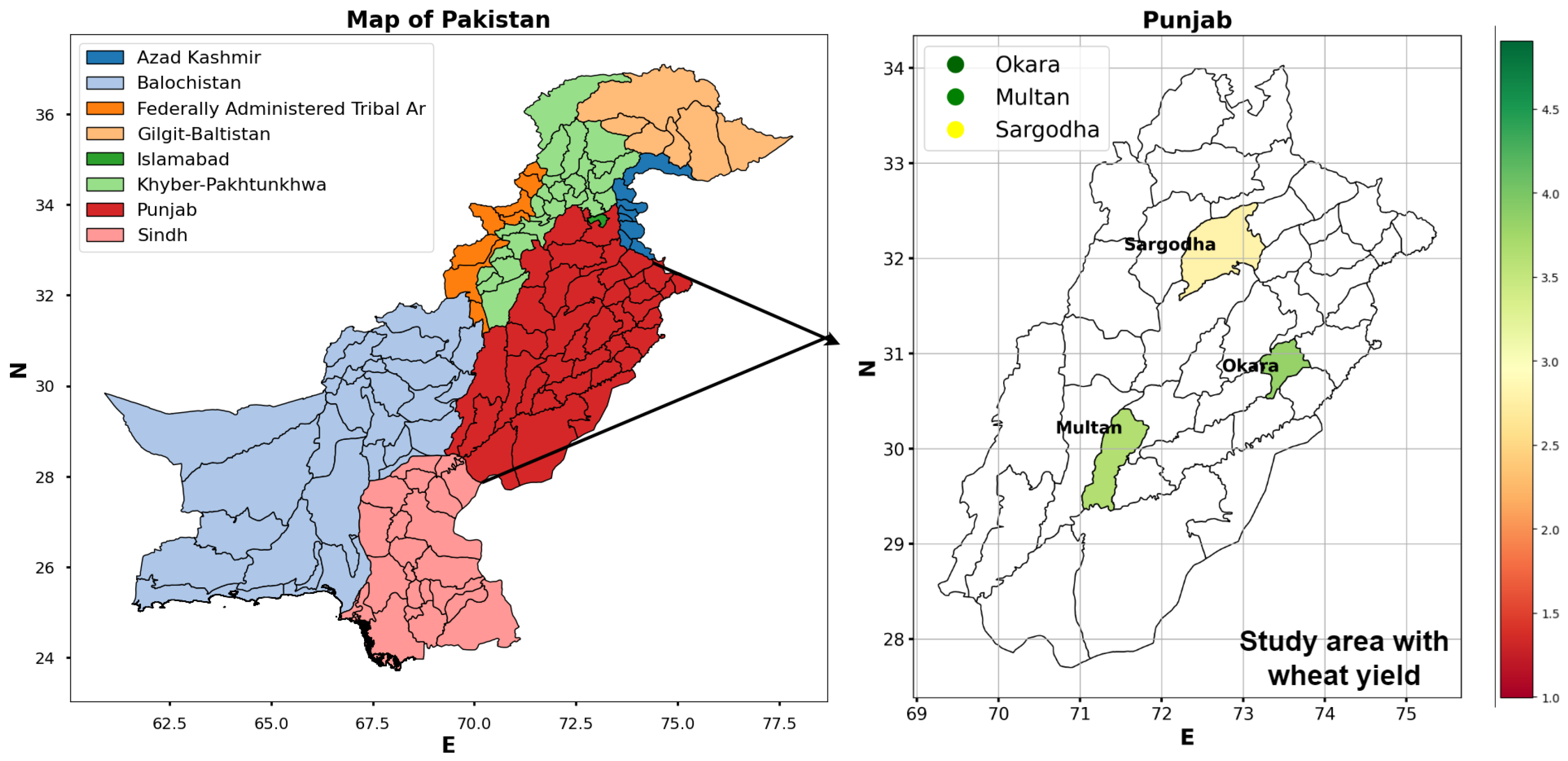
2.2. Study Area

The Okara, Multan, and Sargodha districts in Punjab province were chosen for their significant contributions to wheat production. The study area with wheat yield is mapped in Figure 2. Okara district, located in central Punjab at latitude $30.{8138}^{°}$ N and longitude $73.{4534}^{°}$ E, spans 2969 square kilometers. It boasts fertile agricultural lands irrigated by the Sutlej River and its tributaries, making it an ideal region for wheat cultivation. Multan district, situated in southern Punjab at latitude $30.{1575}^{°}$ N and longitude $71.{5249}^{°}$ E, covers an area of 3177 square kilometers. Known for its arid climate, Multan provides suitable conditions for wheat cultivation. Sargodha district, positioned in northern Punjab at latitude $32.{0740}^{°}$ N and longitude $72.{6861}^{°}$ E, encompasses 3139 square kilometers. Sargodha is a crucial area for wheat production in the region.

Projected climate changes, including temperature increases and altered rainfall patterns, are expected to significantly impact wheat production by mid-century. From 1980 to 2010, wheat yields fell by 5.5%, with a 0.13 °C temperature rise per decade. By 2050, global wheat output could drop by 1.9%, with severe impacts in Africa and South Asia, where yields might decline by 15% and 16% [27]. Major producers like Pakistan may also see reduced yields, threatening the global wheat supply. This study examines the factors driving climate change and its impact on essential crops like wheat.

2.3. Observed Data

The study utilized meteorological data encompassing monthly rainfall and minimum and maximum temperatures, manually collected from the weather database [28], spanning 1991 to 2021. Additionally, historical wheat-yield data (measured in tons/ha) from producing fields were sourced from the Government of Punjab [29] from 1991 to 2021.

2.4. GCM Data

Global Climate Models (GCMs) are widely recognized for their effectiveness and accuracy in assessing global climate change. In this study, we leveraged ensemble data to forecast future climate conditions in the study area. We collected data for AR4 SRB1, A2, and A1B mean composite emission scenarios from 24 international modeling centers, using baseline years 1971–2012 and 2011–2052. Recent research in climate modeling guided our decision to focus on these three specific GCMs (emission scenarios), particularly due to their suitability for simulating climatic conditions in the Punjab regions [21]. According to this study, these three GCMs are the best options for climatic simulation conditions in the Punjab. The AR4 Intergovernmental Panel on Climate Change provided monthly statistics [30] for 20 years and 30 years, encompassing the same geographic coordinates as the research area.

The IPCC Fourth Assessment Report (AR4, 2007) provided greenhouse gas concentration trajectories for SR emission scenarios. A1B predicted medium emissions, with atmospheric CO₂ levels reaching 703 ppm by 2100. A2 represented high emissions, resulting in 836 ppm CO₂, whereas B1 simulated lesser emissions, with CO₂ at 540 ppm in 2100. The study retrieved monthly climatic variables at a $0.{25}^{°}$ resolution, downscaled from three GCMs under the above-mentioned scenarios. Data collected included total precipitation (mm/day), maximum and minimum near-surface air temperature (°C), average air temperature (°C), surface downward motion shortwave heat (W/m²), and average wind speed at 10 (m/s). The XGboost model is employed to downscale GCM and observed data as predictors. The XGboost was chosen for its effective performance in solving nonlinear problems [18,31].

2.5. Data Processing

The methodology for data preprocessing and crop-yield projections involved several key steps. Data were gathered from various sources, processed, and used to calibrate models and validate results. To provide robust analysis, missing or irregular values must be addressed carefully.

Firstly, daily historical weather data, including maximum and minimum temperature and rainfall, was collected from a weather database [28]. Following the validation of the daily climatic data, several quality checks were carried out to assure reliability. These checks included data validation against preset acceptable ranges, logical sequence consistency tests (for example, temperature consistency), interpolation to handle missing data, and removing duplicate records. To manage missing data, linear interpolation was utilized, with each missing value estimated by averaging the values before and after it. To maintain data integrity, duplicate records were identified, and only the first instance of each duplicate entry was retained. This was then aggregated into monthly averages to match the timelines of the future estimates. The processed historical monthly climate datasets were combined into a single Excel file with pertinent modeling inputs and transformed into annual averages. The time series data yielded a uniform length of 31 years of records for each region.

The climate-prediction data utilized in this study were obtained from GCM AR4 for three future emissions scenarios: SRA2, B1, and A1B. The data were originally stored in netCDF format and must be preprocessed before analysis. We used Google Colab (Python) to convert the netCDF files to comma-separated values (.csv) for easy use in spreadsheet tools. As a result, Excel’s filtering tools allow us to reduce our focus to certain geographic places relevant to our research. Detailed documentation and metadata are critical for cooperation, comprehension, and validation. LAT and LONG filters were used to separate the study areas from the data. At first, the numbers were shown as monthly means over 20 or 30 years. Before making predictions about the average temperatures and amounts of rain and snow from 2022 to 2052, we changed them to yearly means.

The original GCM data were in Kelvin, but our history data are in degrees Celsius (°C), so we changed them. We need to change information so that they are consistent with each other so that we can make useful comparisons. Also, to match previous records, the amount of rain was changed from kg/m²/h to mm. The suggested ensemble forecasting method used both estimates about the future and data from the past to give a more accurate picture of how climate affects wheat yields. This method helps us understand seasonal changes and long-term climate trends better by focusing on bigger patterns instead of small changes that happen every day. This method could help farmers and farming groups make better decisions.

Data Splitting

ML models are less likely to be biased when datasets are split up. We carefully split our temperature and yield data into training and testing groups so that we could build models that could accurately predict crop yields. The dataset is split into training and testing groups so that different split ratios can be used to test how accurate the model’s predictions are. Nguyen (2021) says that the ratios of training to tests were as follows: 10–90, 20–80, 30–70, 40–60, 50–50, 60–40, 70–30, 80–20, and 90–10. We tried to avoid overfitting by giving the model the right amount of time to be trained and tested. We used an 80/20 split to train the model with $80\%$ of the data. The other 20% were saved so that we could test the out-of-sample model. This method makes sure that our models will be able to handle new data while they are being tested, which will give us a fair idea of their performance.

For datasets with between 100,000 and 100,000 records, our downscaling scoring method used a 60:20:20 split. In particular, around 60% of the data were used for training the model. A separate 20% portion were the test set for assessing model predictive performance. The final 20% constituted an independent validation set, allowing us to fine-tune hyperparameters. The training set enabled our models to learn underlying patterns from historical data. Hyperparameter tuning was guided by the validation set, optimizing model performance. By exploring various split ratios, we comprehensively understood our model’s forecast ability under different conditions. This exploration informed our final model selection, ensuring robustness when applied at scale.

2.6. Experimental Setup

For developing the machine learning models, historical daily weather data (including minimum temperature, maximum temperature, and rainfall) from 1991 to 2021 and corresponding wheat-yield data were obtained from the weather database and the Government of Punjab. The data were divided into 80% training and 20% testing sets. Six different supervised learning algorithms were used—artificial neural networks (ANNs) with LR, GFF, PNN, and MLP architectures, MLR, RFR, boosted tree regression, and a stacking ensemble model. The ANN models were developed using the Keras library in Python (specifically, Google Colab) with the Adam optimizer, binary cross-entropy loss, and varying numbers of hidden layers (10–7). They were trained for 90–1100 epochs on this architecture.

MLR was performed using the sci-kit-learn library. The boosted tree models were developed with maximum depth (from 10 to 90), learning rate (0.01), number of estimators (ranging from 100 to 1500), and 8-fold cross-validation. RFR model was built using maximum depth ranging from 10 to 90, several estimators of 80, and cross-validation of 8-fold. A GFF model was created using dense layers of (100, 92, 1) for the ANN. We used ’relu’ activation, ’adam’ optimizer, and ’lbfgs’ solver for training in Keras.

Lastly, a stacking ensemble model was created for training using the weighted average of the base models in sci-kit-learn. Final model evaluation was conducted on the unseen testing dataset, using performance metrics such as mean absolute error, root mean squared error, $R^2$, normalized root mean square error, mean biased error, and correlation coefficient to select the optimal hyperparameters for each algorithm. Regression graphs are generated using the matplotlib library in Google Colab to visualize the performance of all models.

The coarse resolution is downscaled by three GCM outputs from CMIP3 using the XGboost algorithm to project yields under future climates. XGboost was trained on 60% of the weather data for parameter tuning, validated on 20%, and tested on the remaining 20% to map large-scale climate variables to local observations. Hyperparameters such as maximum tree depth 30 and estimators ranging from 4 to 6 were optimized through 2-fold cross-validation. The downscaled climate projections were inputs to the top-performing ML models selected earlier. XGboost demonstrated vital skill in bridging global and regional scales, with downscaled outputs closely matching the validation data distribution. This validated XGboost’s ability to learn complex non-linear relationships between weather factors and crop yields and translate them to future conditions. Its efficient tree ensemble approach allowed for seamlessly incorporating climate model projections into crop forecasts.

3. Machine Learning Algorithms

The wheat-yield prediction was conducted using a range of algorithms, including ANN(LR), ANN(PNN), ANN(GFF), boosting tree, MLR, RFR, and ensemble methods, in conjunction with climate variables. These algorithms were chosen based on their proven effectiveness, as evidenced by previous research studies [16,18,32,33].

3.1. Multiple Linear Regression

Multiple linear regression models demonstrate the connection using a linear equation. One or more accessible (or predictive) variables can be related to a distinct reliant (or responsive) variable, i.e., every independent variable Xi is associated with the dependent variable Y. The multiple regression equation takes the following generic form:

$$Y=\alpha +{\gamma }_1{X}_1+{\gamma }_2{X}_2+{\gamma }_3{X}_3+\eta$$

(1)

where Y is the yield variable; $X_1$, $X_2$, and $X_3$ denote the rainfall, $T_{m}ax$, and $T_{m}in$, respectively; ${\gamma }_1$, ${\gamma }_2$, and ${\gamma }_3$ stand for the rainfall $\gamma$, $T_{m}ax$$\gamma$, and $T_{m}in$$\gamma$, respectively; and $\eta$ is the error in the observed value.

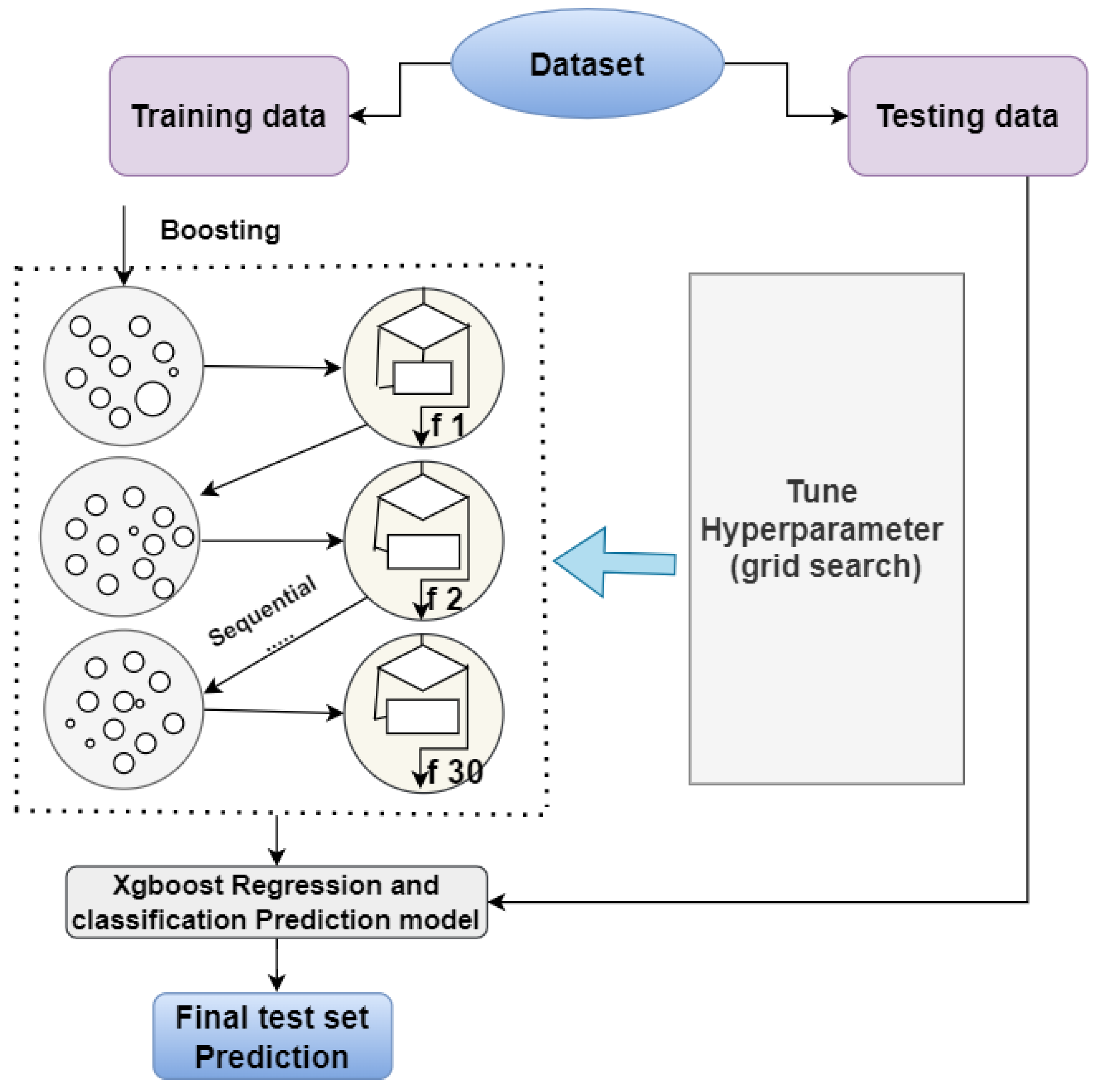
3.2. XGboost

Chen and Guestrin proposed the XGboost technique, a specific gradient boosting approach [34]. In Figure 3, one tree is included while developing sequential trees to optimize the goal further. The model combines slow learners’ predictions to generate a high learner using additive training procedures based on boosting. The model utilizes parallel calculations to enhance speed. It has the excellent fitting abilities of an ensemble tree, which is extremely effective (at most ten times quicker than RF to train) [9]. The fundamental form of the prediction at point t is given in this order:

$$f_i^t=\sum _{k=1}^t{f}_k\left(X_i\right)=f_i^{(t-1)}+f_t\left(x_i\right)$$

(2)

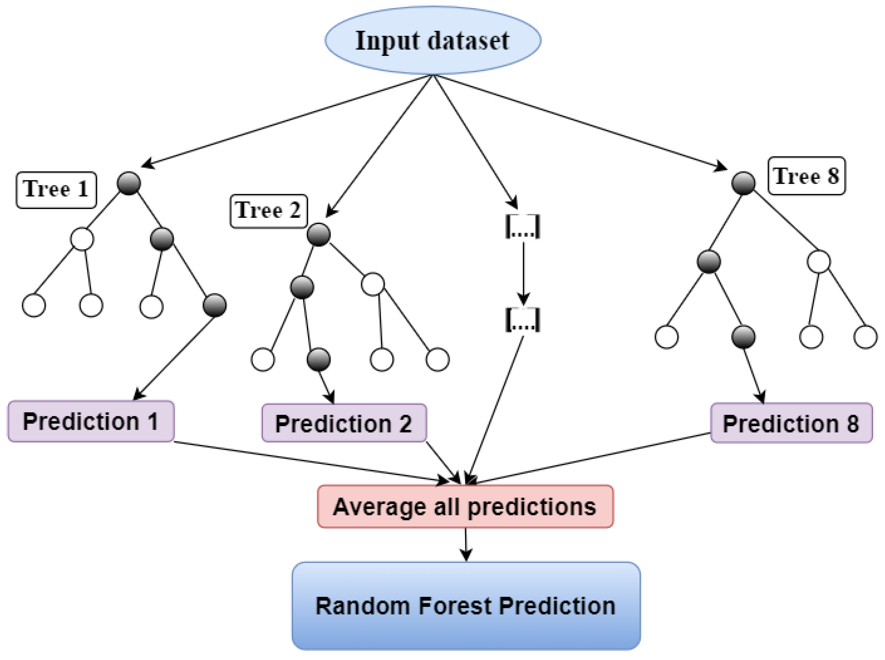
3.3. Random Forest Regression

RFR is a popular technique for digitization because of its capacity to handle complex datasets with non-linear correlations and intricate feature relationships. The model resists excessive fitting, and value gaps are suitable for noisy and incomplete data [35]. The RF algorithm uses many decision forests, each created using random sample data for training and covariance, as shown in Figure 4. The models have the advantage of picking prospective variables and training data for every split, minimizing overfitting, and improving prediction accuracy. Additionally, the model indicates the significance of each variable employed in the prediction. We used the Scikit-learn toolkit’ to identify RF features and important functions and rank the value of specific features in our RFR models. This helped us to grasp the fundamental processes that impact model reliability and yield. It was optimized through 20-max depth with a minimum splitting size of 2. The margin function for the training dataset taken at random from the distribution of the random vectors X, Y, and an ensemble of classifiers $h_1\left(X\right),h_2\left(X\right),\cdots ,h_k\left(X\right)$ is as follows:

$$mg(x,y)=a{v}_{k}I(h_k\left(x\right)=Y)-maxa{v}_{k}I(h_k\left(X\right)=j)$$

(3)

where I(.) is the indicator function. The margin measures the extent to which the mean number of votes at X and Y for the correct class exceeds the mean vote for any other class.

3.4. Artificial Neural Networks (ANNs) Model

An ANN is a nonlinear machine learning approach (Figure 5). The network comprises three interlinked layers: input (nodes), hiding (one to three layers of neurons), and output. Each link is assigned a numerical value known as its weight. Neuron j in the deep layer produces the output $h_j$ [36].

$$h_j=\sigma \left(\sum _{i=1}^N{V}_{ij}{x}_i+T_j^{hjd}\right)$$

(4)

In this equation, $\sigma$ represents the simulating function, N represents the count of input neurons, $V_{i}j$ represents the weight, $x_i$ represents the neuron input, and $T_j^{hjd}$ represents the hidden neuron threshold.

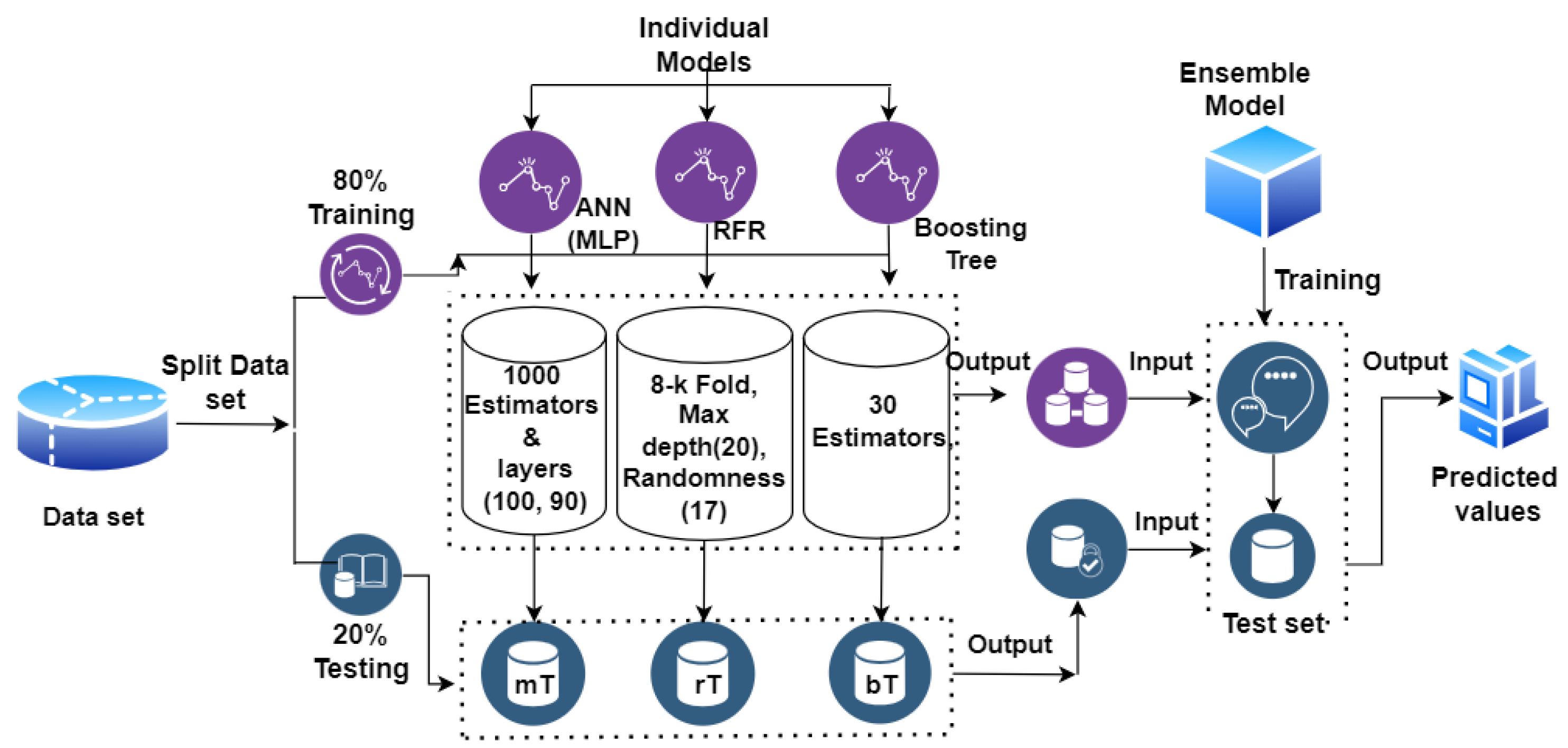
3.5. Ensemble Model

Anurag Satpathi [20] and Xuan Yang [37] compared traditional ML models to improved ensemble models. Ensemble models are highly precise as they mix numerous varieties of a single method to aggregate predictions from many basic learners. In the present research, we have employed three models to develop an ensemble model: random forest regression, ANN (multilayer perceptron), and boosting tree. The algorithm steps of the ensemble model for the wheat-production system diagram are shown in Figure 6.

The multilayer perceptron model is trained with 1000 n-estimators, using input and output layers (100, 90). The RF model is trained with altered parameters on eight folds (excluding fold1), and the fold1 results are forecasted. Repeating this technique eight times generates predicted values in the training set. For RF, we set max-depth to 20 and randomness to 17. The Boosting Tree model is trained with 30 estimators and randomness set to 24.

The training batch now comprises three sets of expected values combined to generate a new training set. The trained RF, ANN(MLP), and boosting tree models are applied to predict three sets of projected values for the test set (containing N3 samples). Finally, these three trained models train and validate a secondary layer ensemble model. The test sample is fed into the prepared ensemble model, which produces its final predicted result. This ensemble approach improves the accuracy of predictions and generalization, addressing the limitations of individual machine-learning techniques in crop-production prediction.

3.6. Evaluation Metrics

A machine learning model’s performance is assessed using several statistical measures that quantify how closely the model predicts the results. Metrics guide us during model fine-tuning and hyperparameter optimization and provide insights into various aspects of model accuracy, reliability, and potential biases [38]. The mean absolute error (MAE), correlation coefficient (R), root mean squared error (RMSE), mean biased Error (MBE), normalized root mean square error (MSE), and normalized mean square error (NMSE) were utilized to assess the downscaling capabilities [39,40]. Better model performance is indicated by $R^2$ and R near 1 and by values of MAE, MBE, and RMSE close to zero. Positive MBE values suggest overestimation, whereas negative values imply underestimating. The model effectiveness is categorized as outstanding, good, fair, or poor based on the nRMSE value, which ranges from 0 to 10%, 10 to 20%, 20 to 30% or >30%, respectively. The statistics index formulas are provided below:

$$MAE={\displaystyle \frac{1}{j}}\sum _{i=1}^j|x_i-\acute{x_1}|$$

(5)

$$\mathrm{NMSE}=ln\sum _{i=1}^j\left[{\displaystyle \frac{{(x_i-{\acute{x}}_i)}^2}{\left(\widehat{x_i}\widehat{{\acute{x}}_i}\right)}}\right]$$

(6)

$$RMSE=\sqrt{{\displaystyle \frac{{\sum }_{i=1}^N{(x_i-{\widehat{x}}_i)}^2}{N}}}$$

(7)

$$MBE={\displaystyle \frac{1}{n}}\sum _{i=1}^N(x_i-{\widehat{x}}_i)$$

(8)

$$nRMSE=\sqrt{{\displaystyle \frac{{\sum }_{i=1}^N{(x_i-{\widehat{x}}_i)}^2}{N}}}*{\displaystyle \frac{100}{\widehat{\acute{A}}}}$$

(9)

$$R={\displaystyle \frac{{\sum }_{i=1}^N(y_i-{\widehat{y}}_i)({\acute{y}}_i-\widehat{{\acute{y}}_i})}{\sqrt{{\sum }_{i=1}^N{(y_i-{\widehat{y}}_i)}^2{\sum }_{i=1}^N{(y_i-{\widehat{\acute{y}}}_i)}^2}}}$$

(10)

Here, $x_i$, $y_i$ is the observed yield values, ${\acute{x}}_i$, ${\acute{y}}_i$ is the produced yield values for the $i^{th}$ value, ${\widehat{x}}_i$, ${\widehat{y}}_i$ and ${\widehat{\acute{x}}}_i$, ${\widehat{\acute{y}}}_i$ indicate the median values of the pertinent factors, N denotes the amount of data points analyzed. To evaluate downscaling performance, $x_i$, $y_i$ and ${\acute{x}}_i$, ${\acute{y}}_i$ show historical and downscaled meteorological variables. The model’s capacity to generate the yield of wheat function and downscaled meteorological parameters for the research area is evaluated using a linear regression $y=\alpha x+\gamma$. The variable that is dependent (y) is the response (or target) variable, while the independent variable (x) is the predictor (or feature) variable. The intercept is $\gamma$, and the slope is $\alpha$. The wheat-yield function is evaluated by regressing observed and forecasted yield data.

4. Results

The results of the proposed machine learning models concentrate on:

• Conduct a correlation analysis between climate factors and wheat yields and identify the climate variables most significantly correlated with wheat production through statistical hypothesis testing of relationships.
• Apply various machine learning models (RF, MLR, boosting tree, MLP, PNN, GFF) to the historical climate and wheat-yield data to generate predictions and compare against actual historical yields.
• Evaluate the various machine learning models using training performance metrics such as $R^2$, R, nRMSE, MAE, MBE, and RMSE to identify the best performers.
• To downscale coarse resolution GCM climate projections to local scales under three emission scenarios (SRA1B, SRB1, SRA2) using the XGboost statistical downscaling model.
• Applying the best-performing machine learning model to project wheat yields over periods for three locations and emission scenarios using the downscaled generated climate variables data.

4.1. Importance of the Climate Parameters on Wheat Yield

Descriptive statistics for all variables are summarized in

Table 1. Descriptive statistics.

Locations	Variables	Statistics
		Average	Minimum	Maximum	Standard Deviation	SE	Skewness	CL
Okara	Rainfall	500.65	301.78	836.2	139.57	25.07	0.540	27.87
	$T_{max}$	32.48	30.83	33.83	0.818	0.147	0.2794	2.520
	$T_{min}$	21.00	19.50	22.25	0.618	0.11	0.132	2.946
	Yield	3.428	2.5006	3.904	0.416	0.074	−0.878	12.15
Sargodha	Rainfall	725.62	477.30	1131.7	173.52	31.165	0.511	23.91
	$T_{max}$	31.59	29.83	33.16	0.860	0.154	0.123	2.723
	$T_{min}$	20.59	18.25	21.91	0.965	0.173	−1.13	4.689
	Yield	2.613	2.194	2.994	0.259	0.046	−0.270	9.926
Multan	Rainfall	337.68	169.30	553.8	114.94	20.64	0.089	34.04
	$T_{max}$	33.02	31.33	35.00	1.019	0.183	0.3685	3.086
	$T_{min}$	21.74	20.08	23.41	0.902	0.162	−0.389	4.14
	Yield	2.822	1.996	3.647	0.456	0.0820	0.020	16.18
All sites	Rainfall	521.31	169.3	1131.7	214.59	22.25	0.550	41.16
	$T_{max}$	32.36	29.83	35.0	1.07	0.11	0.263	3.313
	$T_{min}$	21.11	18.25	23.41	0.96	0.099	−0.434	4.555
	Yield	2.954	1.99	3.904	0.517	0.0536	0.2281	17.50

.

Okara experiences moderate rainfall (average 500.65 mm), while Sargodha receives higher rainfall (average 725.62 mm). Multan has the lowest rainfall (average 337.68 mm). Overall, the combined average rainfall across all sites is 521.31 mm. Okara has an average $T_{max}$ of 32.48 °C, Sargodha averages 31.59 °C, and Multan experiences higher temperatures with an average $T_{max}$ of 33.02 °C. The overall average $T_{max}$ is 32.36 °C. Okara’s $T_{min}$ averages 21.00 °C, Sargodha at 20.59 °C, and Multan at 21.74 °C. The overall average $T_{min}$ is 21.11 °C. Okara has the highest yield (average 3.428), followed by Multan (average 2.822) and Sargodha (average 2.613). The overall average yield is 2.954. Sargodha stands out for high rainfall but lower yield, while Multan experiences the highest temperatures. Okara strikes a balance between these factors.

Table 2. Importance of the climate parameters.

Location	Variables	${\mathit{Coefficient}}^{\mathit{p}}$	Covariance	SE	R	t (Value)	p (Value)	95% Confidence Level
								Lower	Upper
Okara	Rainfall	−0.0001	0.000	0.006	0.1842	−0.104	0.9179	−0.001	0.001
	$T_{max}$	−0.0629	0.010	0.101		−0.620	0.540	−0.271	0.145
	$T_{min}$	0.114	0.017	0.131		0.869	0.3921	0.155	0.383
Sargodha	Rainfall	0.0001	0.000	0.0003	0.7106	0.2646	0.793	−0.0004	0.0005
	$T_{max}$	0.084	0.002	0.0517		1.627	0.115	−0.021	0.190
	$T_{min}$	0.154	0.001	0.040		3.869	0.0006	0.072	0.236
Multan	Rainfall	0.0003	0.0000	0.0006	0.6976	0.5365	0.5960	−0.0008	0.0014
	$T_{max}$	0.1185	0.007	0.086		1.3698	0.1820	−0.058	0.2958
	$T_{min}$	0.2482	0.009	0.0965		2.5722	0.0159	0.050	0.446
All sites	Rainfall	0.000	0.000	0.0002	0.149	0.310	0.757	−0.000	0.001
	$T_{max}$	0.116	0.004	0.066		1.766	0.081	−0.015	0.248
	$T_{min}$	0.114	0.004	0.066		1.734	0.086	−0.071	0.246

demonstrates how climate conditions influence wheat yields in different locations.

The results of statistical hypothesis testing (p-values) indicate the maximum temperature variable significantly influences wheat-yield responses. This finding is reinforced by analyzing the correlation and covariance relationships between climate factors and yield data. As shown in Table 2, there is a negligible negative coefficient (−0.0001) for rainfall. Still, it is statistically insignificant (p = 0.9179) in Okara, suggesting that these parameters do not substantially impact the local climate variables. In Sargodha, rainfall has a slight positive coefficient (0.0001) and is also statistically insignificant (p = 0.793). Similarly, in Multan, rainfall has a positive coefficient (0.0003) but lacks statistical significance (p = 0.5960). Overall, the impact of rainfall on yield appears minimal across all sites. $T_{max}$ has a favorable coefficient in all locations (ranging from 0.084 to 0.1185). However, only the coefficient for $T_{min}$ in Multan is statistically significant (p < 0.05), indicating its critical role in the region. Higher maximum temperatures may affect wheat yield. $T_{min}$ has positive coefficients in all locations (ranging from 0.114 to 0.2482). The coefficient for $T_{min}$ in Sargodha is statistically significant (p < 0.001). $T_{min}$ likely plays a role in wheat yield, especially in Sargodha.

Meanwhile, the p-values lacked significance for the relationships tested in Okara. The R-values from linear regression models using rainfall, maximum, and minimum temperature as predictors ranged from 0.1842 to 0.7106 across locations. Given the study area’s climate-yield dataset characteristics, this suggests that linear regression may not be the optimal approach for modeling crop yields. The results show that increasing temperatures hurt the wheat yield. Our results correlate with previous research, suggesting that rising heat stress due to climate change will affect wheat yield and production [41,42]. These results emphasize the need for region-specific climate models and localized climate adaptation strategies. Future research should explore these regional differences and underlying mechanisms further.

4.2. Selection of Predictors and Predicted Variables

Wheat-production functions were developed based on environmental factors, including rainfall, minimum temperature ($T_{min}$), and maximum temperature ($T_{max}$) as shown in Figure 7. The dataset used for yield modeling contained climate variables (predictor values) and recorded yield observations (response values). Various ML techniques were applied to model the relationships between climate drivers and wheat yields, including multiple regression, boosted tree regression, artificial neural networks, random forest modeling, and ensemble methods. The objective was to compare the performance of these statistical and ML approaches for projecting crop production under changing climatic conditions.

4.3. Performance Metrics of Different MLA

After implementing the ML models in Google Colab using existing libraries, we achieved the results provided in

Table 3. Statistical comparison of calibrated yield response functions among research models.

Rank	Model	MAE	RMSE	nRMSE %	MBE	R	${\mathit{R}}^2$
1	ANN(LR)	0.305	0.361	24.3	0.013	0.746	0.446
2	ANN(GFF)	0.220	0.301	19.2	−0.180	0.888	0.663
3	ANN(PNN)	0.422	0.466	28.4	−0.190	0.659	0.321
4	MLR	0.307	0.361	24.3	0.012	0.746	0.440
5	Boosting Tree	0.198	0.253	20.0	0.010	0.902	0.741
6	ANN(MLP)	0.230	0.266	17.0	−0.049	0.902	0.739
7	RFR	0.182	0.227	18.0	0.030	0.909	0.791
8	Ensemble	0.099	0.107	8.0	0.022	0.988	0.953

ANN(LR) = Linear Regression; ANN(GFF) = Generalized Feed Forward; ANN(MLP) = Multilayer perceptron; ANN(PNN) = Probabilistic Neural Network; MLR = Multiple Linear Regression; RFR = Random Forest Regression.

, where the red highlighted model represents the best outcome. The statistical comparison of calibrated yield response functions among different research models reveals that the ensemble model demonstrates the best overall performance, with the lowest MAE (0.099), RMSE (0.107), and nRMSE (8.0%), indicating high accuracy. 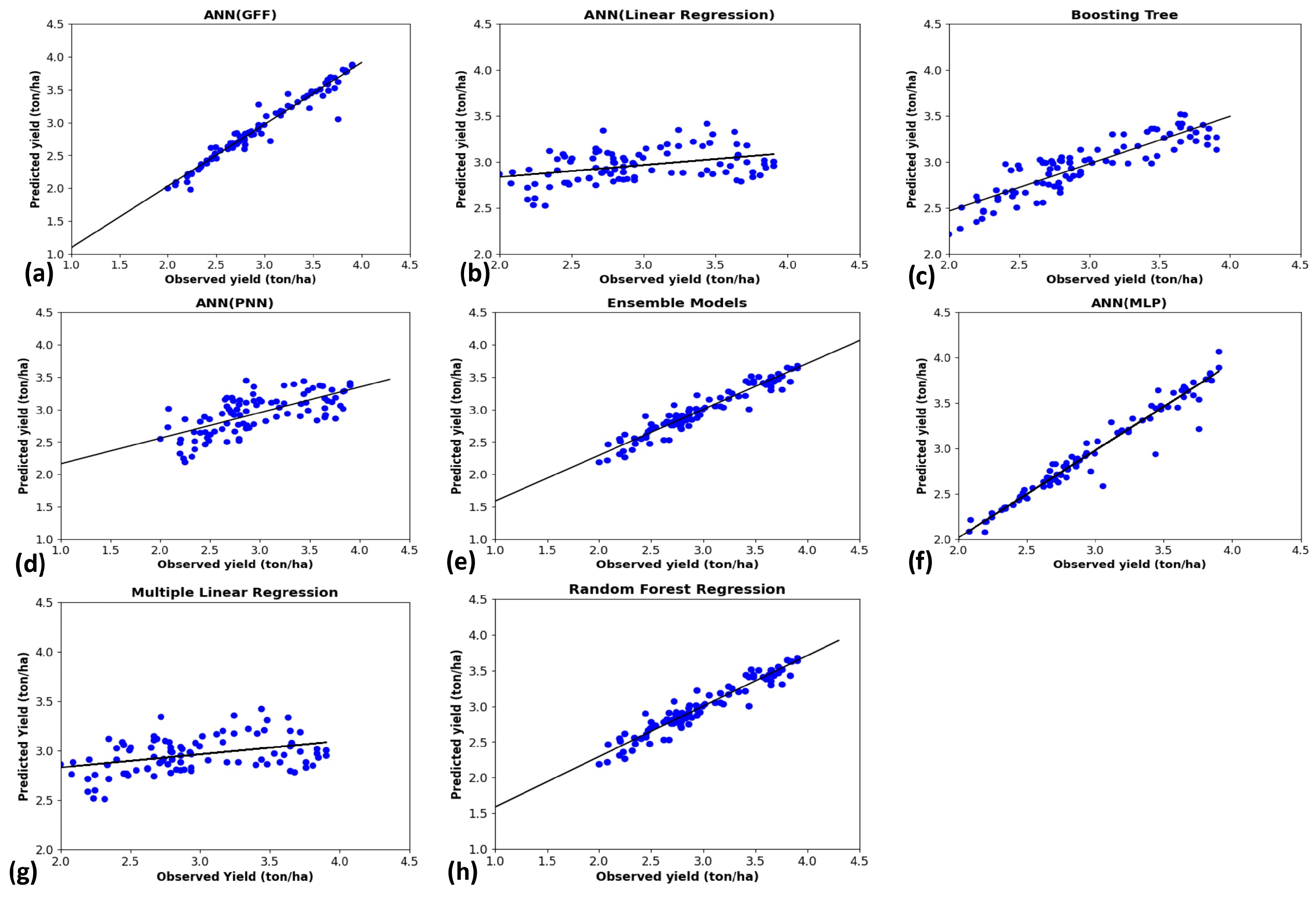It also shows the highest correlation (R = 0.988) and explanatory power ($R^2$ = 0.953), with minimal bias (MBE = 0.022). Following the ensemble model, the RFR and boosting tree models perform well, with RFR having an MAE of 0.182, RMSE of 0.227, and R of 0.909, while the boosting tree has an MAE of 0.198, RMSE of 0.253, and R of 0.902. Both models exhibit low bias and high explanatory power. Among the ANN models, ANN(MLP) shows good performance with an MAE of 0.230, RMSE of 0.266, and R of 0.902, followed by ANN(GFF) with an MAE of 0.220, RMSE of 0.301, and R of 0.888.

In contrast, ANN(LR) and MLR models show similar and moderate performance, each with an MAE of 0.305, RMSE of 0.361, and a correlation coefficient of 0.746. ANN(PNN) exhibits the lowest performance among ANN models, with a high MAE of 0.422, RMSE of 0.466, and a relatively low R of 0.659. The overall analysis indicates that advanced ensemble and tree-based models significantly outperform traditional regression and specific neural network models in accuracy, correlation, and explanatory power, highlighting their suitability for yield response-prediction tasks.

However, the moderate performance of ANN(LR) and MLR and the poor performance of ANN(PNN) highlight that not all neural network configurations are equally effective. These results emphasize the importance of model selection and tuning in achieving optimal predictive performance and suggest that more complex or specialized models offer substantial advantages over more straightforward, more traditional approaches in specific contexts like yield response prediction.

Indeed, the models were ranked in order of performance by the ensemble model, RFR, ANN(MLP), boosting tree, ANN(GFF), ANN(LR), and ANN(PNN) according to a cross-comparison thereof in Table 3. Figure 8 displays the scatter plots of predicted yields against observed yields. The ensemble model performance was deemed adequate since the regression line had a slope close to 1, indicating predictions closely matched observed values. The intercept was nearly 0, showing little overall bias in the model’s estimates. Predicted and actual data points are closely aligned along the 1:1 reference line with minimal dispersion.

Figure 9 compares yield curves for calibrated model outputs and observed data from 1991 to 2021. The ensemble model, ANN(MLP), RFR, and ANN(GFF) predicted time series yield data closely matching the observed yields, as evidenced by the comparing curves. Ensemble modeling showed a particularly strong performance for this climate-yield dataset. Small residual errors and close alignment between ensemble predictions and observations demonstrate its reliable representation of patterns.

According to the model evaluation findings, the ensemble model was the most accurate and sufficiently good to assess future yield change trends for 2021–2052 under different scenarios: AR4 SRA2, B1, and A1B. Consequently, we discovered that the yield function may be expressed using artificial neural network methods based on climate factors. The ensemble model is an effective computational tool for simulating wheat-yield response functions under typical meteorological circumstances.

4.4. Downscaling Climate Projections Using the XGboost Algorithm

We first downscaled climate variables across the study area to project wheat yields under future climates using the averaged ensemble of IPCC AR4 emissions scenarios. This multi-model mean incorporated high (A2), medium (A1B), and low (B1) CO₂ emissions scenarios. The XGboost algorithm was selected to downscale climate data from 1991 to 2052, as prior work has effectively applied it in similar contexts [18]. We employed a 60%, 20%, and 20% split to train, test, and validate the XGboost model on observed historical climate records from 1991 to 2052 for the three regions. Projections from global climate models served as predictors. By downscaling the multi-model mean using XGboost—a method proven skillful by others—we generated high-resolution climate inputs to drive our crop modeling while accounting for emissions uncertainty.

Table 4. Downscaled climate projections from emissions scenarios using XGboost.

Locations/ Scenarios	Training				Testing				Validation
	RMSE	nRMSE %	MAE	R	RMSE	nRMSE %	MAE	R	RMSE	nRMSE %	MAE	R
Okara/B1
$T_{max}$	0.244	0.90	0.102	0.979	0.248	0.90	0.113	0.970	0.210	0.63	0.200	0.970
$T_{min}$	0.222	0.79	0.095	0.991	0.221	0.795	0.099	0.99	0.105	0.485	0.099	0.99
Rain	0.387	0.134	0.04	0.924	0.350	0.134	0.061	0.924	0.095	0.244	0.017	0.924
Multan/B1
$T_{max}$	0.107	0.382	0.045	0.994	0.105	0.385	0.049	0.994	0.210	0.619	0.200	0.994
$T_{min}$	0.303	1.08	0.134	0.908	0.304	1.09	0.148	0.985	0.105	0.462	0.099	0.985
Rain	0.387	0.159	0.025	0.923	0.358	0.159	0.030	0.923	0.067	0.228	0.016	0.920
Sargodha/B1
$T_{max}$	0.197	0.732	0.086	0.989	0.197	0.733	0.086	0.989	0.210	0.658	0.200	0.989
$T_{min}$	0.240	0.827	0.098	0.987	0.238	0.827	0.119	0.942	0.105	0.496	0.099	0.997
Rain	0.416	0.126	0.039	0.909	0.437	0.126	0.044	0.900	0.090	0.172	0.017	0.900
Okara/A2
$T_{max}$	0.220	0.816	0.088	0.984	0.224	0.826	0.097	0.984	0.210	0.638	0.200	0.985
$T_{min}$	0.247	0.884	0.103	0.985	0.246	0.884	0.107	0.986	0.105	0.486	0.090	0.985
Rain	0.123	0.042	0.019	0.993	0.119	0.043	0.028	0.99	0.083	0.211	0.011	0.99
Multan/A2
$T_{max}$	0.257	0.918	0.107	0.973	0.254	0.918	0.117	0.975	0.210	0.619	0.200	0.976
$T_{min}$	0.226	0.810	0.095	0.944	0.227	0.810	0.105	0.983	0.105	0.462	0.099	0.983
Rain	0.073	0.030	0.009	0.99	0.067	0.032	0.011	0.99	0.291	0.983	0.113	0.998
Sargodha/A2
$T_{max}$	0.214	0.794	0.09	0.985	0.214	0.794	0.096	0.986	0.210	0.658	0.200	0.986
$T_{min}$	0.239	0.825	0.096	0.988	0.237	0.845	0.116	0.988	0.105	0.496	0.099	0.988
Rain	0.101	0.030	0.020	0.996	0.106	0.030	0.023	0.996	0.069	0.120	0.011	0.997
Okara/A1B
$T_{max}$	0.294	1.08	0.121	0.966	0.300	1.09	0.135	0.966	0.210	0.638	0.200	0.966
$T_{min}$	0.233	0.834	0.105	0.989	0.232	0.835	0.110	0.980	0.105	0.485	0.099	0.989
Rain	0.285	0.099	0.028	0.958	0.258	0.099	0.042	0.958	0.146	0.372	0.034	0.959
Multan/A1B
$T_{max}$	0.272	0.972	0.117	0.970	0.269	0.972	0.127	0.970	0.210	0.619	0.200	0.970
$T_{min}$	0.254	0.907	0.109	0.983	0.255	0.907	0.119	0.983	0.105	0.462	0.099	0.983
Rain	0.349	0.144	0.026	0.937	0.324	0.144	0.031	0.937	0.105	0.356	0.031	0.937
Sargodha/A1B
$T_{max}$	0.221	0.819	0.094	0.984	0.221	0.819	0.098	0.985	0.210	0.658	0.200	0.985
$T_{min}$	0.369	1.27	0.156	0.953	0.367	1.274	0.189	0.953	0.105	0.49	0.099	0.954
Rain	0.411	0.124	0.070	0.917	0.43	0.124	0.081	0.917	0.069	0.119	0.009	0.918

represents the statistical performance of the XGboost for downscaling all three parameters. All scenarios’ mean error values for $T_{max}$ during training ranged between 0.107 and 0.416 (RMSE), 0.030 and 1.08% (nRMSE), and 0.09 and 0.121 (MAE) (°C). The mean error values for $T_{min}$ during the training ranged between 0.222 and 0.369 (RMSE), 0.79 and 1.27% (nRMSE), and 0.095 and 0.95 (MAE) (°C).

The mean error values for precipitation during the training period ranged between 0.073 and 0.416, 0.159 and 0.174%, and 0.009 and 0.07 (mm/month) for the RMSE, nRMSE, and MAE. R values for $T_{max}$, $T_{min}$, and precipitation ranged between 0.966 and 0.998, 0.908 and 0.99, and 0.909 and 0.993. During testing, overall mean error values ranged between 0.067 and 0.437 (RMSE), 0.030 and 1.27% (RMSE), and 0.010 and 0.200 (MAE), and during validation, accuracy was higher than testing, i.e., 0.067–0.291 (RMSE) and 0.00–0.009 (MAE), respectively. Additionally, the nRMSE value for all three regions in the emission scenario SRB1 for variable $T_{max}$ and rain gives an outstanding performance comparison to the $T_{min}$ variable in the Multan region. In the emission scenario SRA2, the value of nRMSE also indicates outstanding performance for all three region variables.

In the SRA1B scenario, the Okara region performs better for $T_{min}$ and Rain, Multan performs well for all three variables, and Sargodha gives excellent results for Rain. We discovered that the model’s downscaling ability changed with average emission scenarios. Precipitation was downscaled with the SRA2 scenario, providing the highest performance (R = 0.90–0.996). However, SRB1 resulted in R values ranging from 0.909 to 0.92, and SRA1B ranged from 0.917 to 0.957. In SRA2, we also found that Sargodha’s precipitation performance was best, with R = 0.996. $T_{min}$ performance in SRB1 ranged from R = 0.908 to 0.99, in SRA2 from R = 0.944 to 0.988, and in SRA1B from R = 0.958 to 0.989, with SRA1B giving the most accurate performance in Okara (R = 0.989). $T_{max}$ performance in SRB1 ranged from R = 0.979 to 0.994, SRA2 from R = 0.973 to 0.985, and SRA1B from R = 0.966 to 0.984. When evaluating the downscaled temperature projections against observations, the XGboost approach appeared to capture patterns in daily high temperatures more accurately than in daily low temperatures.

The scatter plots comparing downscaled XGboost outputs to observed climate data showed strong, statistically significant correlations. For maximum temperature ($T_{max}$), the model captured between 0.913 and 0.951 of observed variation for Okara, 0.926 and 0.979 for Multan, and 0.951 and 0.961 for Sargodha during training, as seen in Figure 10. Similarly, Figure 11 showed for minimum temperature ($T_{min}$), the R-squared values ranged from 0.863 to 0.950 for Okara, 0.908 to 0.949 for Multan and 0.863 to 0.942 for Sargodha. While performance was higher for $T_{max}$ than $T_{min}$, both remained within acceptable ranges.

Figure 12 Precipitation outputs also correlated strongly with observations, with R-squared values ranging from 0.860 to 0.970 for Okara, 0.861 to 0.925 for Multan, and 0.837 to 0.970 for Sargodha during testing. This confirms that the downscaled projections generated by XGboost capture observed temperature and rainfall patterns with high fidelity, validating its use for impact modeling at local scales under future climates. The XGboost model demonstrated excellent downscaling performance for all variables during training, testing, and validation in the SRA1B, SRA2, and SRB1 scenarios.

The study leveraged the XGboost algorithm to downscale precipitation, minimum temperature, and maximum temperature projections for 2021–2052. These climate variables were derived from the averaged multi-model ensemble of IPCC AR4 baseline simulations. The downscaled climate projections, spanning 2021–2052, served as inputs to the crop-yield-modeling process. Specifically, we utilized these high-resolution climate data streams within the “Ensemble model”, a previously validated yield estimation function shown to achieve the highest accuracy levels.

4.5. Wheat-Yield Prediction over 2052

Our study leveraged the ensemble yield model with statistically downscaled climate variables under three IPCC emissions pathways (A1B, A2, B1). Figure 13 shows the predicted yields over 31 years for Okara, Multan, and Sargodha. Interestingly, while yields varied substantially year-to-year, we observed no statistically significant differences between the scenarios within each site. The yields with SRA1B are $3.30\%$ less than SRA2; SRB1 is also higher than SRA1B and SRA2, with 6.67% and 9.97% in Multan. In Sargodha, SR-A2 is higher than SRA1B and SRB1 at 6.2% and 6%. On the other hand, the greatest values in historical yield were 3.90, 2.99, and 3.64 (ton/ha) for Okara, Sargodha, and Multan. Specifically, field measurements across locations indicated an average peak yield of 0.95 tons per hectare. However, when using climate projections from GCMs within our crop modeling, the average maximum yield forecast was 0.90 tons per hectare, which means that yield decreased by 5.56%. According to these findings, climate change is projected to reduce wheat output in these regions by at least 5.5%. In our research, we discovered that ML models greatly improve the accuracy of wheat-yield predictions. Unlike traditional statistical methods, which struggle to consider the nonlinear and intricate connections between climate variables and crop yield, ML models—especially ensemble approaches—can effectively handle high-dimensional data and capture complex patterns, resulting in more dependable predictions.

The improving accuracy of ML models allows farmers to build better adaptation techniques. Farmers may make informed decisions about planting schedules, irrigation timing, and crop selection based on precise production estimates. These decisions help to increase resistance to adverse climate circumstances. Farmers can protect crop yields by predicting probable losses due to rising temperatures and implementing mitigation measures, such as selecting heat-tolerant wheat cultivars or modifying agricultural practices.

5. Comparison of the Proposed Method with Existing Techniques

The proposed wheat crop-production forecast system should be evaluated against machine learning and deep learning methodologies.

Table 5. Comparison with existing studies.

Ref/Year	Data Type	Methodology	Factors	${\mathit{R}}^2$	RMSE
[45], 2019	Remote sensing data	SVM	Multiple variables, Yield	0.93	11.7%
[43], 2020	Meteorological and remote sensing data	LSTM, CNN	Phenology variables (11) Climate variable (9) Yield	0.77	721 kg/ha
[44], 2020	Satellite images climate data, soil maps Historical yield	AdaBoost model	Vegetation indices $T_{min}$, $T_{max}$, mean soil, 6 other features	0.86	0.51
[46], 2021	Climate and geographical data	SVM	$T_{min}$, $T_{max}$, mean humidity, min-max WS, Yield	0.33	760kg/ha
[39], 2021	Climate, satellite data soil data	LSTM	$T_{min}$, $T_{max}$ precipitation, Yield soil depth/texture, pH.	0.83	561kg/ha
[47], 2022	Multi source data	RFR	SVI, Climate data, Soil properties, Yield	0.74	758 kg/ha
[40], 2022	Climate, GCM(CMIP6) data	Ensemble Model	Temperature Precipitation SPEI, Yield	0.705–0.918	0.358–0.390
[19], 2023	Multi-sensor data	Ensemble model	$T_{max}$, Sunshine duration Precipitation, Irrigation volume	0.692	0.916 t/ha
[25], 2023	Climate data and Remote sensing, SPEI	SVM	$T_{min}$, $T_{max}$ humidity, RH, WS 2-scenarios wheat	0.78	2.07
[22], 2023	in-situ, meteorological, and remote sensing	MLR	Multi-variables, Yield	0.64	733.53 kg/ha
[18], 2023	Multi-source data	XGBoost	LST, NDVI pH, 6 other features, Yield	0.89	0.3
Proposed Work	Climate, GCM(CMIP3) data	Ensemble MLM	${\mathbf{T}}_{\mathbf{min}}$, ${\mathbf{T}}_{\mathbf{max}}$, Rainfall, Yield	0.953	0.107

compares the suggested strategy to the current state of the art, demonstrating its generalizability. When evaluating machine learning systems, accuracy is often the most important factor. Various performance measures, including accuracy, were utilized to assess the efficacy of the classifier under different settings. The proposed deep and machine learning models outperform current methods significantly. Refs. [43,44] achieved good accuracy using deep learning on phenology/vegetation data. However, climate factors were underrepresented. Ref. [40] used an ensemble approach on GCM projections like our study. While accuracy was moderate, incorporating uncertainty estimates through multiple models was a strength. The proposed work achieved exceedingly high performance metrics as compared to previous investigations.

This suggests the fusion of machine learning algorithms within an ensemble modeling framework effectively captured the complex inter-dependencies between climate variables and wheat over climatic conditions. By leveraging a wealth of data from multiple sources, including CMIP3 climate projections, the study was able to train models on a far richer information set than prior research reliant on narrower inputs. This likely empowered the ensemble to uncover intricate linear and non-linear response patterns across locations and periods that simpler individual models could not detect. The R2 (0.953) and RMSE (0.10) metrics surpassed the next-best scores based on the comparison provided. The proposed ensemble models methodology outperformed other machine learning and deep learning methodologies with all factors in Table 5.

6. Discussion

This work presents a novel way to predict wheat yield under climate change scenarios that employs a complex ensemble of machine learning models. The fundamental novelty of this research is the integration of many advanced machine learning algorithms to estimate wheat output based on climate data, which involves utilizing historical climate data as well as projections from GCMs. We applied a range of ML models, including RFR, MLR, boosted tree regression, artificial neural networks (ANNs), XGboost, and ensemble models, to forecast wheat yield to varying climate conditions. Subsequently, observed climate factors and yield data were used to evaluate and refine the predicted wheat-yield function. The downscaled GCMs output for different CO₂ emissions scenarios AR4 SRB1, A2, and A1B were incorporated into the calibrated output response model to anticipate yield trends through 2052. Focusing on local wheat data, our research aims to capture growth characteristics, predict future trends, and enhance crop-yield projections for the specified area.

In our study, we found that maximum temperature ($T_{max}$) and minimum temperature ($T_{min}$) are crucial in influencing wheat yield, while rainfall has minimal impact. Notably, the ensemble model—combining the strengths of various machine learning models—outperformed traditional methods. With an impressive $R^2$ value of 0.953 and an RMSE of 0.107, the ensemble model outperformed individual models in capturing the complicated connections between climatic conditions and crop yield. Policymakers can use insights from ML models to create policies that promote sustainable agriculture practices. For example, prioritizing investments in climate-resilient crop types and encouraging advanced irrigation practices can help to boost agricultural adaptability. Integrating ML models into national agricultural planning allows for more effective resource allocation, which helps to ensure food security in the face of climate change.

Previous research on the impacts of climate change on wheat production in China found that winter wheat yields are projected to decline by 7.1% over the next 50 years, according to their modeling. Meanwhile, their analysis anticipated spring wheat yields will decrease by 17.5% over the same time. This separate study examined the potential effects of global warming, specifically on winter wheat cultivation in Gansu Province, China. Their results revealed little to moderate impacts on the suitable growing region for winter wheat under various climate change scenarios forecasted for the province.

The researchers [48,49] used two regional climate projection models with RCP 4.5 and RCP 8.5 scenarios. The study found that environmental degradation, specifically temperature trends, has a statistically significant impact on crop yield in this region. The impacts analysis found that wheat yields may rise by up to 14% in some areas but fall 7.9–11% in others depending on temperature trends. This demonstrates that climate change, through its effects on warming, presents statistically significant risks to regional agricultural productivity.

The research findings suggest that under projected drought conditions in South Asia, there could be a substantial decrease in wheat yield, with estimates indicating a potential reduction of around 29.30% compared to normal yield levels [40]. By utilizing advanced climate and crop models, the study aims to provide insights into the future risk of yield reduction under different drought intensities, highlighting the significant impact of extreme weather events on crop production in the region. Ref. [50] examined wheat-yield variability under expected future climates using previous wheat-yield sensitivity data. As well [51], this study found that increasing temperature has a detrimental impact on wheat yields, but cumulative precipitation had a favorable impact. Future climate scenarios are expected to increase temperature, decreasing wheat yields in Punjab.

Pakistan has the fourth largest irrigation system globally, contributing around 90% of agricultural production. However, the country lacks sufficient weather observatories across all regions and provinces to properly examine the relationship between climate and agriculture.

Here are some fundamental approaches to improve wheat yield while adapting to changing climate conditions:

• More weather stations are needed across Pakistan to thoroughly examine nationwide climate-agriculture relationships at the district and provincial levels.
• Developing and promoting wheat varieties that exhibit heat tolerance, drought resistance, and disease resilience is crucial. These climate-smart cultivars can withstand extreme temperatures and water scarcity, ensuring stable yields.
• Early sowing and climate-informed planting dates help avoid extreme heat stress during grain filling. Adjusting planting windows based on weather forecasts improves yield outcomes.
• Efficient irrigation systems, rainwater harvesting, and proper water scheduling are essential. Consistent water supply during critical growth stages enhances yield.
• Mapping suitable crop habitats can aid precautionary measures and innovations to boost agricultural output and food security amid climate shifts.

Although our study focused on the Punjab region of Pakistan, the methodologies and models we employed can be adapted to other areas and crops. This scalability underscores the importance of ML models as crucial tools for global agricultural planning and improving food security strategies. Future research could explore applying these models in diverse geographical contexts and with various crops to validate their effectiveness and adaptability. The results will equip policymakers to craft innovative crop-management strategies for crops like wheat and maize locally and nationally. Collaboration across disciplines will increase our collective potential to construct climate-resilient food systems in the face of urgent climate hazards. Future research should consider other variables such as soil health, pest and disease prevalence, and socioeconomic characteristics to improve the robustness and accuracy of crop-production estimates. Furthermore, more complex ensemble approaches and real-time data can improve machine learning models’ adaptability and reactivity. Collaboration among data scientists, agronomists, and policymakers will be critical to realizing the full promise of machine learning in agriculture.

7. Conclusions

The study used various advanced modeling techniques, including random forest regression, BTR, ANN, MLR, and ensemble models, to forecast site-specific wheat-yield responses based on weather conditions and yield data. The ensemble model, RFR, and ANN(MLP) were better than boosted tree regression when it came to calibrating wheat output models for Punjab. The ensemble model did better than the others, with an R2 of 0.953 and an RMSE of 0.107. The study also showed that artificial neural networks are good at predicting crop yields in both current and future climate scenarios. This was achieved by using GCM results for many CO2 emission scenarios to do this up until 2052. The study found that higher temperatures in Punjab are more to blame for lower wheat yields than lower temps. According to the study, higher temperatures during key stages of growth may lead to lower wheat yields. You cannot say enough about how important it is to think about the highest temperatures when making climate-resilient plans to protect world farming output and ways of making a living. The yield response model we used is based on downscaled GCM predictions. It shows that under different climate change scenarios, wheat yield will drop by 5.5% by 2052. Because of climate change, wheat output is going down, which shows how important it is to have flexible growing methods. Make climate forecasts for the years up to 2052 by putting together the results of global warming models with different scenarios for CO2 emissions. By incorporating machine learning (ML) models to predict wheat yield under climate change scenarios, we gain several advantages over traditional methods. These models offer improved predictive accuracy, enabling us to guide adaptation strategies and inform policy decisions. Their transformative potential in agriculture underscores the importance of advanced data analytics. As we progress, refining these models and exploring their applicability across diverse regions and agricultural systems will be crucial for ensuring global food security.

Our research identified a need for more research on crop prediction in specific areas of Pakistan, particularly regarding wheat-yield forecasting in Punjab using GCM data. This study explores machine learning models’ potential in enhancing wheat-yield prediction in these regions. Through advanced techniques applied to agricultural data, our research contributes to understanding climate change impacts on agriculture, offering crucial insights for developing targeted adaptation strategies in Punjab, Pakistan. Our interdisciplinary approach underscores the importance of collaborative efforts in addressing climate change challenges to global food security, providing actionable insights for policymakers, agricultural experts, and farmers to develop adaptive measures and resilient crop management practices.