1. Introduction
Energy harvesting has been a central concern in human technology historically and continues to be so today. This includes the practice of harvesting energy from motion [
1,
2]. A basic principle of energy harvesting from motion created by humans, such as our body motion or vehicle motion, is to harvest energy that is otherwise lost as friction [
2] so that one gains energy without impeding the desired motion. A potential source for such energy is the undesired vertical motion of vehicle bodies, which is presently typically lost as heat in the suspension system.
There is accordingly significant research into harvesting energy from suspension systems (see Refs. [
3,
4,
5] for reviews). There are proposals involving variable damping coefficients [
6], active suspension [
7,
8], regenerative control [
9], and more [
5,
10,
11,
12]. There are several companies undertaking research on suspension harvesting (see, for example, Refs. [
13,
14]).
A crucial question in such research is how much energy can be extracted. The rough amount of energy available in passenger cars is estimated at 100–400 W [
15,
16]. The amount of energy that can potentially be recovered from the suspension depends on both the car and the road parameters. Understanding this dependence is important for judging the feasibility of suspension harvesting and what the optimal power outputs are.
In this article, we provide several results concerning the possible power output from the suspension as a function of the road and vehicle parameters. We employ numerical and analytical tools, including stochastic processes models and system dynamics methods [
17]. We employ the widely used quarter car model which is regarded as accurate while not being too complex [
18,
19]. In the quarter car model, one models a quarter of the car, as illustrated in
Figure 1. We model the road either as having randomly distributed uneven bumps or speed bumps. The model we propose using for randomly distributed bumps is known as the AR(1) process (autoregressive model of order 1) [
20]. In this process, there are random changes in the vertical profile of the surface, as well as a degree of memory of the surface at the previous point. We show that this model matches the ISO 8608 standard [
21] for road roughness well. We find that the road roughness coefficient of ISO 8608 and the diffusion coefficient of the AR(1) road are equal up to a factor. We model replacing the resistive dampening in the suspension with an energy harvester. This approach is chosen so that the energy harvesting does not impact the motion differently to a normal suspension. We consider both resistive loads and supercapacitor loads. We provide numerical simulations and analytical expressions concerning how much power can be extracted for the given road and vehicle parameters.
2. One Speed Bump
This section concerns how much power can be extracted from a single speed bump. We firstly describe the simulation model and then analyse how much power can be harvested when the car goes over the bump.
2.1. Simulation Model
We model a speed bump by generating a road height
, where
H is the maximal height,
L is the length,
v is the car speed, and
t is the time. The bump is depicted in
Figure 2. We use this model because it is stated to be a good approximation for the commonly used circular speed bump [
22,
23].
In the simulation, the harvester replaces the damper
c shown in
Figure 1. We employ the paradigm that only energy otherwise dissipated as heat may be harvested, such that the motion of the vehicle is not altered relative to the normal suspension when the harvester is introduced. Whilst in some circumstances, such as water wave energy harvesting [
24], it can be advantageous to optimise power output by maximising the motion, in the case of vehicle suspension, this is clearly not desired. The damping force from the harvester is modelled as
, where
. This
models the scenario of a resistive load connected to an EM harvester as described in
Appendix A. The case of a supercapacitor as the load is considered in
Appendix C. The damping force conducts infinitesimal work
on the quarter car with associated power
. Energy conservation then means that
is the maximal power that can be generated by the harvester in the process. The energy generated
E is the instantaneous power
P integrated from the moment of hitting the bump to when the motion induced by the bump stops.
The energy harvested E depends on the bump and car parameters. Unless stated otherwise, the simulations for the speed bump employ the following parameters: Ns/m, Ns/m, N/m, 135,000 N/m, kg, kg, m, and m. These were chosen to match a low-speed electric vehicle such as an E-Trike (a three-wheeled low-speed electric vehicle).
In this section on speed bumps, we use Simulink [
25] to calculate the energy harvested from the relative motion of the car body and the wheel. The associated state-space model is described in
Appendix A.
2.2. Most Power Is Available When Passing the Bump
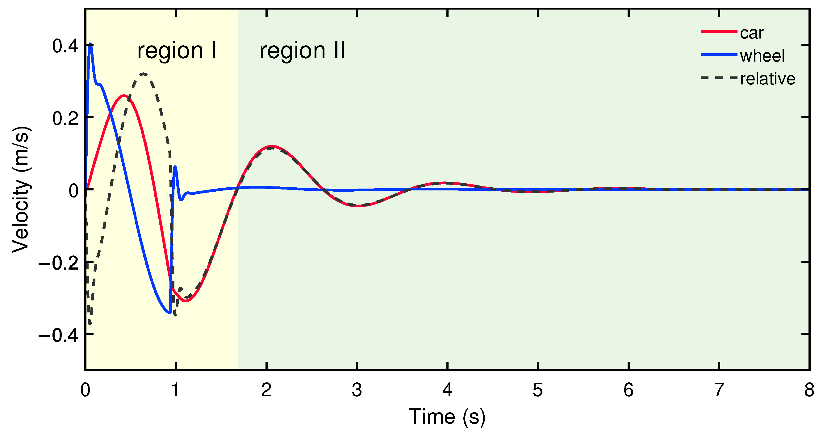
In
Figure 3, we see a typical output of a simulation, divided into ‘being over the bump’ (region I) and ‘having passed the bump’ (region II), respectively. The wheel is initially accelerated quickly in region I; the suspension translates this into a smoother motion of the car chassis, consistent with a significant relative motion between the chassis and wheel. It is from this relative motion that one can gain power by damping the motion with a transducer.
Figure 4 shows how most energy is harvested at two moments associated with entering and exiting the bump. It moreover shows that there is a band of damping coefficients from
to
, with higher and lower values relative to that band yielding less. Intuitively, those extreme values of
c lead to the energy being dissipated in the wheel instead of being harvested.
2.3. How Harvested Power Depends on Speed, Damping Constant, and Bump Parameters
Very different values, ranging from 3000 N
s /m to 11,000 N
s /m, of the damping coefficient
c give rise to maximal power for different speeds, as shown in
Figure 5. For example, if in the 40 km/h case
c was assigned to be 3110 Ns/m, for which the harvested energy from a quarter car model moving at 15 km/h is maximal, the harvested energy would be 229.27 J, taking up 72.15 % of that harvested by setting
, which is 317.75 J. The speed bump simulations show that the height of the bump has little to no effect on which
c maximises the power harvested, whereas the length of the bump does (see
Appendix B).
Next, we turn towards a road with randomly distributed bumps of varying heights and a more analytical treatment.
3. Random Road Surface
We now consider suspension energy harvesting given a road model corresponding to imperfections rather than well-structured speed bumps. A simple approach to model a random road is to pick the height from a Gaussian distribution (also called the Bell curve or Normal distribution) at each position x (for some discretisation of x). However, physical surfaces tend to have smoother changes, so we consider a generalisation of a Gaussian road modelled by an autoregressive process, as will be explained below. We use the generalised model to derive an expression for how much power can be extracted as a function of the parameters involved. The derivation involves, for technical convenience, Fourier transforming the road surface and then working in the frequency domain.
3.1. Model of Generalised Gaussian Road AR(1)
We assume the road surface can be modelled by the autoregressive process AR(1) [
26]. The term ‘autoregressive’ stems from the fact that the current value of the process is regressed upon (or predicted from) its own past values. The number 1 indicates that only the most recent time value is used. More specifically,
where
is the height of road at position
x,
is the distance between road height samples,
d is a decay parameter, and
is a normal distribution function independent of
x, with the mean 0 and standard deviation
.
Applying Equation (
1) iteratively
n times obtains
where each
is picked independently with the mean 0 and standard deviation
.
We shall later encounter ratios of the parameters
d,
, and
associated with the AR(1) road. We will mainly focus on the regime where
d is close to 0, since we will show that the AR(1) model matches the ISO standard for characterising road roughness in that regime. We note that, for small
d, two ratios of AR(1) parameters are expected to directly correspond to physical properties of the road and not be artefacts of the sampling spacing
. Consider replacing
with
. Then, (i)
d changes to
for small
d from Equation (
2) and (ii)
changes to
. Therefore, the ratios
and
remain constant under such sample interval replacement. Keeping in line with common terminology of stochastic processes in physics, we term
D the diffusion constant and
the decay rate.
The impact of the road surface on the quarter car relative velocity
can be more conveniently calculated in terms of sinusoidal decompositions. The derivatives in the Newtonian equations of motion are easy to calculate for sinuisodal functions of time. We shall therefore make use of the Fourier transform of the road surface. To distinguish it from other heights, we shall label the road height
(and the heights of the two masses as
and
where
). Since the car travels with speed
v, for time
t,
whether
i is 1, 2,
r, or
. There is accordingly one Fourier transform of
associated with the
x parametrisation,
and another associated with
t as follows:
We shall analyse how each Fourier component of the road is associated with the Fourier component of the relative motion of the same frequency. A Fourier component of the road with weight in the Fourier decomposition will turn out to be required by the equations of motion to have a fixed ratio with a Fourier component of the relative motion. This ratio is termed the transfer function of the two given Fourier components. The potential power output will be proportional to . We next calculate , known as the spectral power density of the road, followed by calculating the transfer function .
3.2. Spectral Power Density of Generalised Road
We will derive the expression of the spectral power density [
27]
for the generalised Gaussian road AR(1), where the notation “
” denotes a definition.
We start with the fact that the spectral power density
is the Fourier transform of the autocorrelation function:
where
is termed the autocorrelation of
. Equation (
5) follows from noting that
and from letting
. (See, for example, Ref. [
26] as a background reference on such calculations.)
To evaluate the integral in Equation (
5) for our case of an AR(1) road, we firstly calculate the autocorrelation function. Given the AR(1) assumption of Equation (
1) and recalling that the assumption implies Equation (
2), the autocorrelation of the road can be obtained by
The last equality in Equation (
6) can be recovered as follows.
. Demand
. Then,
, such that
.
We now wish to use Equation (
6) to evaluate Equation (
5).
When
, let
and define
, where
. Then
, such that the term in Equation (
5) is proportional to
Thus, combining Equation (
7), Equation (
6) and Equation (
5) one sees that
When
, from Equation (
1), we have
, which corresponds to white noise. A white noise road profile has distribution
and is commonly stated as having autocorrelation
(where
is the unit impulse function), such that
Equation (
9) can, reassuringly, also be recovered as a limit of the following computationally well-defined
discrete Fourier transform of Equation (
6):
From Equation (
10), when
,
.
3.3. Relation to ISO Standard for Characterising Road Roughness
In the ISO 8608 standard, the road profile is characterised in terms of the power density spectral density
[
21] as a function of the spatial angular frequency
. If we again let
x represent the longitudinal position of the vehicle and
represent the road height above the reference line at
x, then
and
, where ‘
’ denotes a definition. The ISO 8608 standard [
21] involves the curve-fitting assumption that
Here,
is the spatial angular frequency, and often
rad/m.
C is a coefficient that can be interpreted as the road roughness. The ‘waviness’
is a somewhat controversial value, which may depend on
and is often set as 2 for simplicity [
28]. The formula for
then only has one free parameter, which is the roughness coefficient
C.
We are now in a position to derive
of Equation (
11) from the assumption of the road being generated by AR(1), as defined in Equation (
1).
For a small decay rate,
,
, and
. Then, from Equation (
8),
where the second approximation assumes that
.
D is the diffusion rate of the road. When comparing with Equation (
11), we find that the road roughness coefficient of ISO 8608 and the diffusion coefficient of the AR(1) road are equal up to a factor:
4. Energy Harvested on a Random Road Surface
We firstly derive the transfer function which captures how different the frequency components of the road surface are associated with the relative motion of the car body and wheel. We then use the transfer function to derive the power dissipated as a function of the car and road parameters.
4.1. Transfer Function on a Gaussian Road
Transfer functions play a crucial role in analysing and optimising suspension systems (see, for example, Ref. [
17]). For a given sinusoidal input with a given frequency, there is a certain output response of the given frequency, and the transfer function in question is the ratio of the output and input amplitudes. In our case, the input is the road surface and the output is the relative motion of the car body and tire.
The relevant transfer function of the quarter car model can be derived as follows. Firstly, write down the Newtonian equations of motion for the quarter car:
where the terms are as defined in
Figure 1. Fourier transforming both sides, and writing for notational simplicity
, yields
Equation (
15) can be seen in a few lines (see
Appendix E) to yield a transfer function
, respecting
Equation (
16) corresponds to a resistive load coupled to the EM harvester. In
Appendix C, we moreover derive an alternative transfer function
H corresponding to a supercapacitor as a load.
We can now write down the transfer function for a common choice of car parameters. The
golden car is a quarter car model used in the international road roughness index (see
Appendix D) with specific parameter values given in
Table 1. Taking that case as an example, Equation (
16) reduces to
where the golden car parameters are denoted as
,
=
/
,
/
,
/
, and
/
[
29].
The power density spectrum of the relative motion of the golden quarter car is, for any quarter car, given in terms of the power density spectrum
Next, we will apply Equation (
17) and Equation (
18) to calculate the energy dissipation in the damper/harvester.
4.2. Potential Power Output
The instantaneous power dissipated in the damper/harvester can be written in terms of the relative motion of the tire and car body as
. Taking the stochastic average yields
where the second equality assumes that the average relative velocity, without conditioning on known previous values, is 0.
Moreover, noting that
and, as shown earlier, the known fact that
one sees that
can be written as
Plugging Equation (
8) and Equation (
16) into Equation (
24) yields
By putting in, for example, the golden car parameters, Equation (
25) becomes
Furthermore, for the golden car speed used in the IRI road roughness index,
m/s, the integral of Equation (
26) can be evaluated analytically with Mathematica to yield
where
is defined as
and
is the diffusion constant of the AR(1) process. For concreteness, suppose
and that the golden car parameters are used. For a golden car with
kg, the energy dissipated from Equation (
19) is then
The above argument exemplifies how, in general, plugging Equation (
25) into Equation (
19) yields an analytical expression for the expected power as a function of the parameters of the quarter car model and the AR(1) road model. This is a key technical contribution of this paper.
We can also, as a further example, evaluate the power when the road model reduces to AR(0). From Equation (
8), the power spectrum is then
. Similar to Equation (
26),
which leads to the power of the golden car of
kg and
m to be
The golden car example can further be used to relate the International Roughness Index IRI for roads [
29,
30] to the extractable power of that golden car, as detailed in
Appendix D.
5. Summary and Outlook
We investigated how much power can be harvested from the suspension of a vehicle. We assumed the paradigm of converting the energy otherwise dissipated as heat into work. We firstly investigated how much power can be harvested from a semicircular speed bump, finding that most power is harvested whilst passing the bump rather than in the oscillations after it, and that the harvested amount depends on the relation between the damping coefficient to the speed and the length of the bump. We then proposed a generalised Gaussian stochastic model for roads: AR(1). Under the AR(1) assumption, we derived an analytical expression for the amount of power that can be extracted as a function of the parameters of the car and road model. For a special case of AR(1) and a standard car known as the golden car, the extractable power can be directly determined from the International Roughness Index of the road. Another special case of AR(1) allows us to derive a key assumption underlying an ISO standard for characterising road roughness, such that parameters from the ISO standard, together with a free parameter of AR(1), can be employed to analytically calculate the extractable power.
Our findings should help evaluate the potential for energy harvesting from vehicle suspension across a range of road conditions. The results also suggest that the standard characterisations of roads should be augmented to include both free parameters in the AR(1) model. Furthermore, preliminary results not described here suggest that convolutional neural networks can significantly enhance the harvesting by controlling the damping coefficient efficiently, something which deserves further investigation. In particular, dynamically varying damping parameters should be investigated. Furthermore, the assumption of linear systems could be relaxed. Our analytical methods should be extended to more complicated non-linear damping forces from the harvester. The analytical results here should be compared with experimental data. The investigation can also be viewed as contributing to the general program of understanding how much power can be extracted from pseudo-random power sources [
31,
32].
Author Contributions
Conceptualization, O.D. and D.E.; methodology, H.G., W.Z.; software, W.Z. and H.G.; validation, O.D., D.E. and F.M.; formal analysis, H.G.; resources, O.D.; writing—original draft preparation, H.G. and W.Z.; writing—review and editing, O.D., F.M. and D.E.; supervision, O.D. All authors have read and agreed to the published version of the manuscript.
Funding
We acknowledge support from the National Natural Science Foundation of China (Grants No. 12050410246, No. 1200509, No. 12050410245), City University of Hong Kong (Project No. 9610623) and the Shenzhen Science Technology and Innovation Commission (Grant No. 20200805101139001).
Informed Consent Statement
Not applicable.
Data Availability Statement
All relevant data is shown in the article.
Acknowledgments
We thank Hessner Technologies Limited in HK Science Park, Pietro Mincuzzi at Troublemaker and Emil Jersling for discussions concerning energy harvesting from suspension of low-speed electric vehicles.
Conflicts of Interest
The authors declare no conflicts of interest.
Abbreviations
| Symbol | Description |
| v | Speed of the car |
| Damping coefficient of the suspension |
| c | Damping coefficient of the suspension |
| Damping coefficient of the tire |
| Damping force of the suspension |
| z coordinate of the car body |
| z coordinate of the tire |
| Relative displacement between the car body and the tire |
| z coordinate of the road |
| Fourier transformation of in the spatial angular frequency domain, |
| Fourier transformation of in the temporal angular frequency domain, |
| Mass of the car body |
| Mass of the tire |
| Spring constant of the suspension |
| Spring constant of the tire |
| H | Height of the speed bump |
| Transfer function |
| L | Length of the speed bump |
| W | Work conducted on the suspension |
| P | Power of the suspension damping |
| Spectral power density function |
| Spatial angular frequency |
| Temporal angular frequency |
| C | Road roughness |
| Road waviness |
| Normal distributed random variable with mean 0 and variance |
| d | A decay parameter used in AR(1) Gaussian road |
| Variance |
| |
| Sampling distance of the Gaussian road |
| Decay rate of the AR(1) Gaussian road |
| D | Diffusion costant for the AR(1) Gaussian road |
| for the golden car |
| / for the golden car |
| / for the golden car |
| / for the golden car |
| / for the golden car |
Appendix A. State Space Model of Quarter Car
Appendix A.1. State-Space Model of Vertical Car Body Motion
Differential equations of the quarter car model:
The state vector
, and the State-space model can be written as
State-Space Model with Harvester
In this model, we assume that an electromagnetic harvester is installed between car body and wheel and harvesting energy from the relative motion of the two parts. An example model for the instantaneous electrical power generated by the system is [
33]
where
| N | —turns of coil |
| B | —average flux density in the air-gap |
| Nl | —effective length of coil |
| RL | —resistance of load |
| Rc | —resistance of coil |
| Lc | —inductance of coil |
| j | —imaginary unit |
| ω | —angular frequency of relative motion. |
Assuming that the contribution from the inductance of the coil is negligible, this can be simplified as
Appendix B. Different Bump Lengths
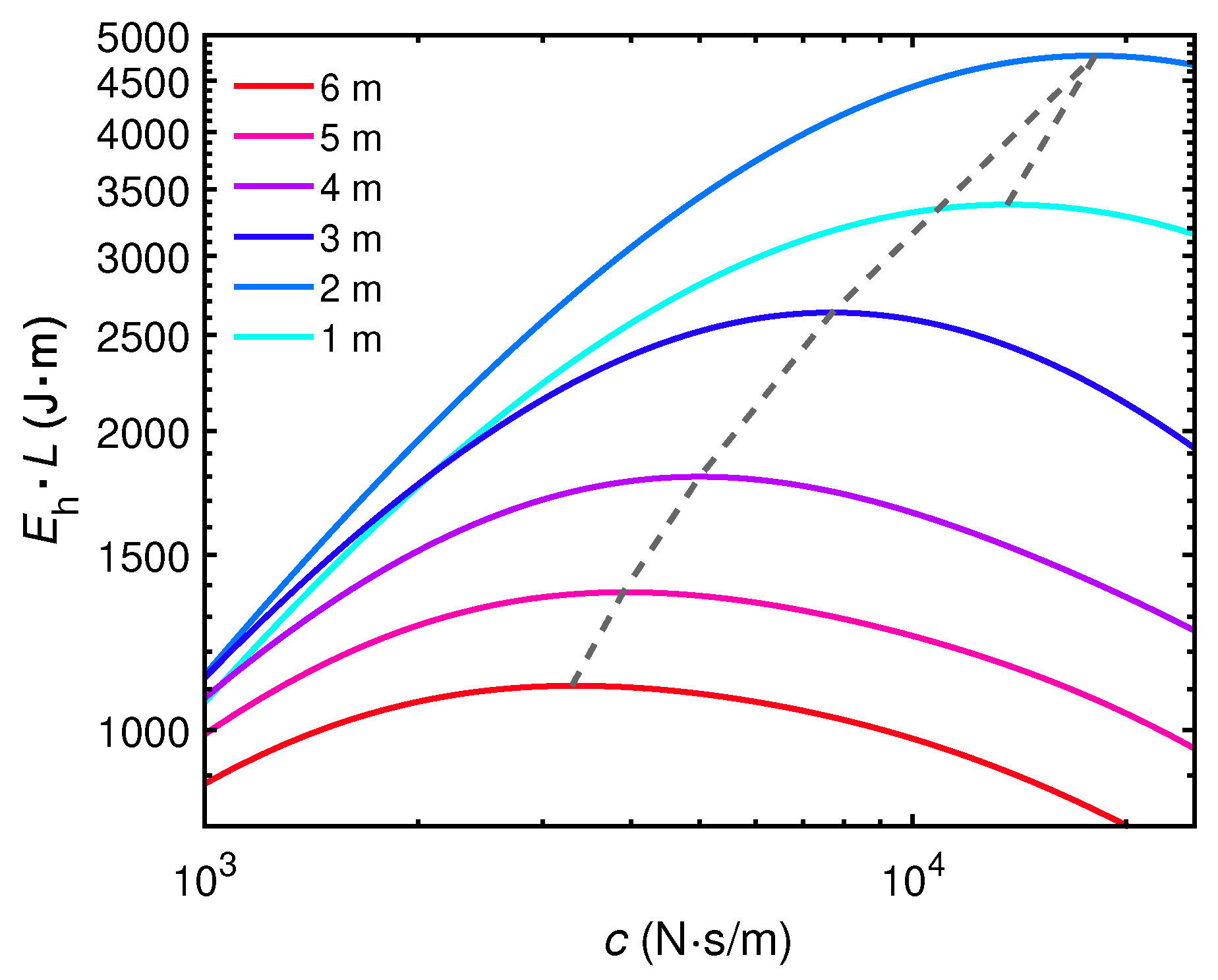
Consider that the height of the speed bump is m. The bump length is set to be 1, 2, 3, 4, 5, and 6 m, respectively. The quarter car is moving at 20 km/h.
From
Figure A1, a strong dependence between which
c maximises the power output and the length of the speed bump are observed.
Figure A1.
Impacts of c on harvested energy for different bump lengths L (1–6 m). The harvested energy is scaled by the bump length for enhancing visibility, and a dashed line connecting maximum values is included for guiding the eyes.
Figure A1.
Impacts of c on harvested energy for different bump lengths L (1–6 m). The harvested energy is scaled by the bump length for enhancing visibility, and a dashed line connecting maximum values is included for guiding the eyes.
Appendix C. Em Harvester Coupled with a Supercapacitor
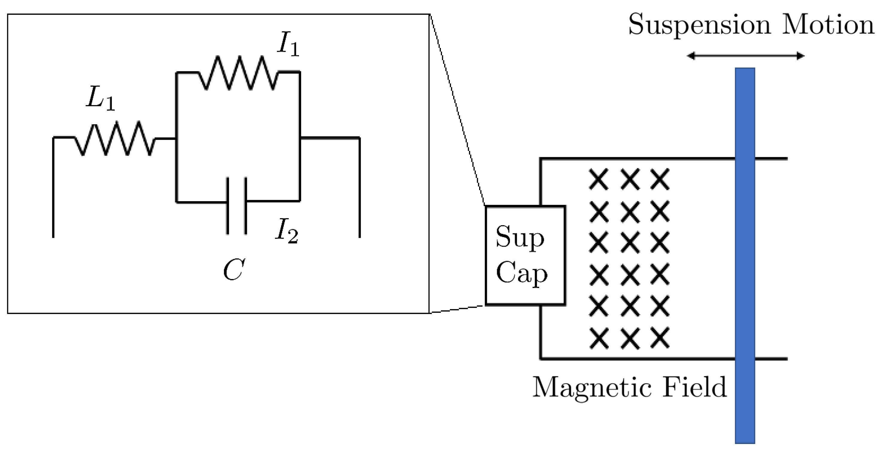
We now consider what change of the load is not resistive, but a supercapacitor. This is motivated by low-speed electric vehicle applications. The simplified set-up we consider is depicted in
Figure A2.
Figure A2.
A simplified EM harvester circuit. The rod cutting the magnetic induction line has a velocity proportional to the relative velocity of the tire and chassis. The generated electric energy is stored in a supercapacitor for quick charging and discharging.
Figure A2.
A simplified EM harvester circuit. The rod cutting the magnetic induction line has a velocity proportional to the relative velocity of the tire and chassis. The generated electric energy is stored in a supercapacitor for quick charging and discharging.
We firstly write down the equations governing the time evolution.
f is the force from the supercapacitor and harvester onto the tyre and chassis. Capital letters indicate Fourier transform, e.g.,
F is the Fourier transform of
f.
Fourier transforming the EM force
f gives
where
We now, armed with the Fourier transform of
f, return to the equations of motion. Firstly, we rewrite them as
Simplifying and Fourier transforming gives
which may be abbreviated as
such that the transfer function of interest is
Appendix D. IRI Relation to Power
The International Roughness Index (IRI) is a common indicator of pavement roughness. It is defined as the difference between the total displacement
L (in meters) of the body suspension and the driving distance, in kilometers, of the golden car standard vehicle driving at the speed of
km/h [
29,
30]: IRI
.
The IRI is closely related to the integral of the power dissipated , but there is a subtlety in that IRI uses the absolute value without the power of 2.
We make the significant assumption that is approximately identically and independently distributed such that . This assumption is for mathematical convenience but can be physically justified in a regime where the suspension response time is much faster than the road variations.
Let
for notational simplicity, then
Thus, taking into account the definition IRI
[
29,
30], we find
where
.
, and the IRI of airport runways, for example, is
, and for rough roads is
.
Although the derivation of Equation (
A14) includes a strong i.i.d. assumption, numerics suggest that the equation holds arbitrarily well for AR(0) roads, indicating that it should be possible to derive Equation (
A14) without that strong assumption.
Appendix E. Transfer Function Given AR(1) Road Details
The transfer function of the quarter car model can be derived as below. The motion equation of quarter car is
Taking the Fourier transformation of both sides and defining
, we have
When simplifying it, we obtain
When solving the above equations, we obtain
The energy harvested by the suspension is directly related to the relative displacement between the car body and the tire,
. Then, we calculate the transfer function
that tells us the relative displacement
based on the road profile
,
References
- Holdren, J.P. Population and the energy problem. Popul. Environ. 1991, 12, 231–255. [Google Scholar] [CrossRef]
- Priya, S.; Inman, D.J. Energy Harvesting Technologies; Springer: Berlin/Heidelberg, Germany, 2009; Volume 21. [Google Scholar]
- Hrovat, D. Survey of advanced suspension developments and related optimal control applications. Automatica 1997, 33, 1781–1817. [Google Scholar] [CrossRef]
- Wei, C.; Jing, X. A comprehensive review on vibration energy harvesting: Modelling and realization. Renew. Sustain. Energy Rev. 2017, 74, 1–18. [Google Scholar] [CrossRef]
- Abdelkareem, M.A.A.; Xu, L.; Ali, M.K.A.; Elagouz, A.; Mi, J.; Guo, S.; Liu, Y.; Zuo, L. Vibration energy harvesting in automotive suspension system: A detailed review. Appl. Energy 2018, 229, 672–699. [Google Scholar] [CrossRef]
- Li, S.; Xu, J.; Pu, X.; Tao, T.; Gao, H.; Mei, X. Energy-harvesting variable/constant damping suspension system with motor based electromagnetic damper. Energy 2019, 189, 116199. [Google Scholar] [CrossRef]
- Karnopp, D. Active and semi-active vibration isolation. In Current Advances in Mechanical Design and Production VI; Elarabi, M.E., Wifi, A.S., Wifi, A.S., Eds.; Pergamon: Oxford, UK, 1995; pp. 409–423. [Google Scholar]
- Suda, Y.; Nakadai, S.; Nakano, K. Hybrid suspension system with skyhook control and energy regeneration (development of self-powered active suspension). Veh. Syst. Dyn. 1998, 29 (Suppl. 1), 619–634. [Google Scholar] [CrossRef]
- Okada, Y.; Harada, H. Regenerative control of active vibration damper and suspension systems. In Proceedings of the 35th IEEE Conference on Decision and Control, Kobe, Japan, 13 December 1996; IEEE: Piscataway, NJ, USA, 1996; Volume 4, pp. 4715–4720. [Google Scholar]
- Zhang, Z.; Zhang, X.; Rasim, Y.; Wang, C.; Du, B.; Yuan, Y. Design, modelling and practical tests on a high-voltage kinetic energy harvesting (eh) system for a renewable road tunnel based on linear alternators. Appl. Energy 2016, 164, 152–161. [Google Scholar] [CrossRef]
- Hoo, G.K. Investigation of Direct-Current Brushed Motor Based Energy Regenerative Automotive Damper. Master Thesis, Department Mechanical Engineering, National University of Singapore, Singapore, 2013. [Google Scholar]
- Faiz, J.; Ebrahimi-Salari, M.; Shahgholian, G. Reduction of cogging force in linear permanent-magnet generators. IEEE Trans. Magn. 2009, 46, 135–140. [Google Scholar] [CrossRef]
- 2006. Available online: https://www.speedgoat.com/success-stories/speedgoat-user-stories/clearmotion (accessed on 5 August 2024).
- 2006. Available online: www.audi-mediacenter.com/en/photos/detail/the-innovative-shock-absorber-system-from-audi-new-technology-saves-fuel-and-enhances-comfort-36880 (accessed on 5 August 2024).
- Zuo, L.; Zhang, P.-S. Energy harvesting, ride comfort, and road handling of regenerative vehicle suspensions. J. Vib. Acoust. 2013, 135, 011002. [Google Scholar] [CrossRef]
- Fairbanks, J. Vehicular thermoelectrics: A new green technology. In Proceedings of the 2011 Directions in Engine-Efficiency and Emissions Research (DEER) Conference, Detroit, MI, USA, Coronado, CA, USA, 3–8 January 2011. [Google Scholar]
- Karnopp, D.C.; Margolis, D.L.; Rosenberg, R.C. System dynamics: Modeling, Simulation, and Control of Mechatronic Systems; John Wiley & Sons: Hoboken, NJ, USA, 2012. [Google Scholar]
- Türkay, S.; Akçay, H. A study of random vibration characteristics of the quarter-car model. J. Sound Vib. 2005, 282, 111–124. [Google Scholar] [CrossRef]
- Alleyne, A.; Hedrick, J.K. Nonlinear control of a quarter car active suspension. In Proceedings of the 1992 American Control Conference, Chicago, IL, USA, 24–26 June 1992; IEEE: Piscataway, NJ, USA, 1992; pp. 21–25. [Google Scholar]
- Box, G.E.P.; Jenkins, G.M.; Reinsel, G.C.; Ljung, G.M. Time Series Analysis: Forecasting and Control; John Wiley & Sons: Hoboken, NJ, USA, 2015. [Google Scholar]
- ISO8608; Mechanical Vibration–Road Surface Profiles–Reporting of Measured Data. Standard, International Organization for Standardization: Geneva, Switzerland, 2016.
- Hassan, A.A.; Rakha, H.A. A fully-distributed heuristic algorithm for control of autonomous vehicle movements at isolated intersections. Int. J. Transp. Sci. Technol. 2014, 3, 297–309. [Google Scholar] [CrossRef]
- Obregón-Biosca, S. Speed humps and speed tables: Externalities on vehicle speed, pollutant emissions and fuel consumption. Results Eng. 2020, 5, 100089. [Google Scholar] [CrossRef]
- Todalshaug, J.H.; Ásgeirsson, G.S.; Hjálmarsson, E.; Maillet, J.; Möller, P.; Pires, P.; Guérinel, M.; Lopes, M. Tank testing of an inherently phase-controlled wave energy converter. Int. J. Mar. Energy 2016, 15, 68–84. [Google Scholar] [CrossRef]
- Chaturvedi, D.K. Modeling and Simulation of Systems Using MATLAB and Simulink; CRC Press: Boca Raton, FL, USA, 2017. [Google Scholar]
- Percival, D.B.; Walden, A.T. Spectral Analysis for Physical Applications; Cambridge University Press: Cambridge, UK, 1993. [Google Scholar]
- Youngworth, R.N.; Gallagher, B.B.; Stamper, B.L. An overview of power spectral density (psd) calculations. Opt. Manuf. Test. VI 2005, 5869, 206–216. [Google Scholar]
- Múčka, P. Simulated road profiles according to iso 8608 in vibration analysis. J. Test. Eval. 2017, 46, 405–418. [Google Scholar] [CrossRef]
- Sayers, M.W. Guidelines for Conducting and Calibrating Road Roughness Measurements; Technical Report; University of Michigan, Ann Arbor, Transportation Research Institute: Ann Arbor, MI, USA, 1986. [Google Scholar]
- Sayers, M.W. On the calculation of international roughness index from longitudinal road profile. In Transportation Research Record; 1995; Available online: https://trid.trb.org/View/452992 (accessed on 5 August 2024).
- Halvorsen, E. Energy harvesters driven by broadband random vibrations. J. Microelectromechanical Syst. 2008, 17, 1061–1071. [Google Scholar] [CrossRef]
- Swati; Singh, U.; Dahlsten, O.C.O. Quantifying the value of transient voltage sources. Phys. Rev. Appl. 2022, 18, 054064. [Google Scholar] [CrossRef]
- El-hami, M.; Glynne-Jones, P.; White, N.M.; Hill, M.; Beeby, S.; James, E.; Brown, A.D.; Ross, J.N. Design and fabrication of a new vibration-based electromechanical power generator. Sens. Actuators A Phys. 2001, 92, 335–342. [Google Scholar] [CrossRef]
| Disclaimer/Publisher’s Note: The statements, opinions and data contained in all publications are solely those of the individual author(s) and contributor(s) and not of MDPI and/or the editor(s). MDPI and/or the editor(s) disclaim responsibility for any injury to people or property resulting from any ideas, methods, instructions or products referred to in the content. |
© 2024 by the authors. Licensee MDPI, Basel, Switzerland. This article is an open access article distributed under the terms and conditions of the Creative Commons Attribution (CC BY) license (https://creativecommons.org/licenses/by/4.0/).


