Improved Multi-Objective Beluga Whale Optimization Algorithm for Truck Scheduling in Open-Pit Mines

Abstract

Big data and artificial intelligence have promoted mining innovation and sustainable development, and the transportation used in open-pit mining has increasingly incorporated unmanned driving, real-time information sharing, and intelligent algorithm applications. However, the traditional manual scheduling used for mining transportation often prioritizes output over efficiency and quality, resulting in high operational expenses, traffic jams, and long lines. In this study, a novel scheduling model with multi-objective optimization was created to overcome these problems. Production, demand, ore grade, and vehicle count were the model’s constraints. The optimization goals were to minimize the shipping cost, total waiting time, and ore grade deviation. An enhanced multi-objective beluga whale optimization (IMOBWO) algorithm was implemented in the model. The algorithm’s superior performance was demonstrated in ten test functions, as well as the IEEE 30-bus system. It was enhanced by optimizing the population initialization, improving the adaptive factor, and adding dynamic domain perturbation. The case analysis showed that, in comparison to the other three conventional multi-objective algorithms, IMOBWO reduced the shipping cost from 7.65 to 0.84%, the total waiting time from 35.7 to 7.54%, and the ore grade deviation from 14.8 to 3.73%. The implementation of this algorithm for truck scheduling in open-pit mines increased operational efficiency, decreased operating costs, and advanced intelligent mine construction and transportation systems. These factors play a significant role in the safety, profitability, and sustainability of open-pit mines.

1. Introduction

Truck transportation is one of the main methods used in open-pit mining. In this field, conventional transportation techniques were inefficient, which worsened the effects on the environment and also consumed more energy and posed serious safety risks [1,2]. Truck schedule rigidity and reliance on manual operation frequently result in traffic jams and delays, raising operating expenses and lengthening waiting times [3,4,5]. Furthermore, it has been established that catastrophic geological occurrences such as landslides and ground collapses are dangerous for driver safety [6,7]. Mining transportation systems are going through a revolutionary age due to the rapid development of artificial intelligence and unmanned driving in recent years [8,9,10]. Newer intelligent mining transportation models maximize efficiency and safety while simultaneously consuming less energy [11,12,13]. Efficient data analytics can be used to enhance route planning and scheduling tactics, effectively mitigating truck congestion and minimizing transportation lag, thanks to the systems’ constant monitoring of the logistical dynamics and mining terrain. In particular, the introduction of unmanned mining trucks not only has improved operational safety but also plays a vital role in material transportation, because transportation cost accounts for a sizeable share of mine operating expenses [14,15,16]. Nevertheless, there are certain drawbacks to the present scheduling procedures for the transferring of unmanned mining trucks, including some waiting time during operations and comparatively high shipping costs [17]. Therefore, it is crucial to design and optimize the unmanned mining truck dispatching model for use in open-pit mines in order to decrease operating costs, increase the effectiveness of ore transportation, decrease carbon emissions, and improve overall corporate performance [18,19,20,21,22].

To simulate real-world dispatch situations and develop scheduling models that align with real-world mining operations, researchers have undertaken in-depth investigations on truck dispatching models. In general, this paper focuses on methods for solving these models and optimizing goals [23,24,25,26]. Early research frequently described very simple models that primarily focused on single-objective constraints before progressively expanding to multi-objective, complex constraints. For instance, Temeng et al. developed and validated a nonpreemptive goal-programming approach for truck dispatching to ensure stable ore quality and maximize production [27]. Topal et al. concentrated on cutting overall truck maintenance costs and used case studies to demonstrate the efficacy of the mixed integer programming approach in doing so [28]. In order to solve energy difficulties while achieving production needs, Patterson et al. proposed a domain search-based algorithm to decrease the energy use of trucks and shovels required to reach production targets [29]. Yao et al. constructed a mine truck scheduling model under mixed transportation constraints based on allocation demand [30].

The dynamic and multidimensional nature of truck dispatching in open-pit mines still presents difficulties issues, despite the tremendous efforts of those researchers to introduce helpful algorithms for truck dispatching models, better adapting them to real mining transportation situations [13,18,22,31]. Environmental protection and worker safety are becoming increasingly important in the context of pursuing intelligent and unmanned mining operations. Increasing operational efficiency while minimizing environmental impact and optimizing operational safety has become a critical issue. As a result, appropriate models must be created and put into use that take safety regulations, production demands, environmental protection, technological advancements, and operation efficiency into account.

Integer programming and the linear programming method are frequently presented as solutions to these models [32,33,34]. Numerous studies have used artificial intelligence algorithms to handle truck scheduling issues as a result of the quick advancement of evolutionary computation techniques. In order to provide workable solutions for the allocation and real-time scheduling of mining trucks, for instance, Coelho et al. employed three multi-objective algorithms—2PPLSVNS, MOVNS, and NSGA-II—to solve dynamic truck allocation problems in open-pit mining operations [35]. Practical scheduling solutions were provided by Mendes et al. who proposed a multi-objective evolutionary algorithm for dynamic truck scheduling in open-pit mines [36]. Two multi-objective genetic algorithms were created by Alexandre et al. to handle scheduling schemes that maximize production and minimize expenses while allocating trucks and shovels in open-pit mining operations [37]. Furthermore, while managing multi-dimensional dispatch objectives, traditional algorithms frequently display subpar performance, lengthy calculation durations, and challenges in generating workable scheduling solutions that efficiently support intelligent dispatch systems. Therefore, there is an urgent need to introduce new solutions to address the challenges in solving mining truck scheduling models. Zhang et al. proposed a beluga optimization algorithm by observing a beluga group’s swimming, feeding, and whale-falling activities [38]. Upon evaluation, the algorithm performed well, and case studies on distributed generation (DG) optimization [39], iron ore sintering batching [40], and anti-roll torsion bar optimization [41] were also carried out. Based on these factors, an improved multi-objective beluga whale optimization (IMOBWO) was introduced, wherein the population was initialized and its range expanded using logistic chaotic mapping. Adaptive factors were proposed to improve the algorithm’s capacity for global searches and to quicken the algorithm’s pace of convergence. The algorithm’s solving power was improved by increasing the domain perturbation approach, broadening the pool of potential solutions. The algorithm’s solution power was demonstrated using ten test functions and the IEEE 30-bus problem for thorough assessment before it was ultimately used with a real mining truck scheduling case.

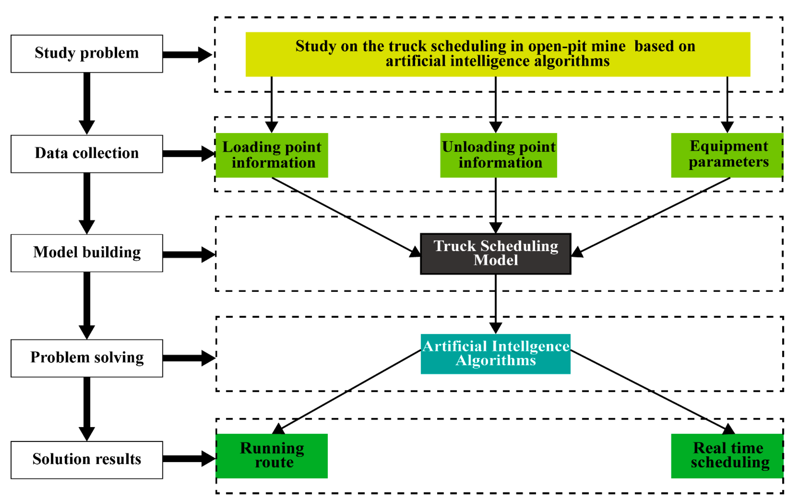
In this study, a new open-pit mine truck scheduling model solved by the IMOBWO algorithm was proposed. The model took production demands, ore grade requirements, vehicle limitations, and route restrictions into account, aiming at achieving comprehensive optimization in terms of carbon emissions, shipping cost, total waiting time, and ore grade deviation. The IMOBWO algorithm performance was evaluated using test functions and the IEEE 30-bus problem, and a scheduling solution was provided following case analysis. This model enhanced operational safety and reduced transportation delays in the mining industry, which was of great significance for improving the overall operational efficiency of open-pit mines.

2. Problem Description and Model Establishment

2.1. Process Analysis of Truck Scheduling Problem

Trucking transportation scheduling is recognized as a multi-dimensional task encompassing path optimization, traffic flow coordination, and dynamic real-time decision making. These dimensions impose significant complexity on the scheduling domain, necessitating the pursuit of varied optimization goals amid numerous constraints. This paper has focused on the achievement of reduced shipping cost, the minimization of total waiting time, and the strict control of ore grade deviation. Furthermore, open-pit mine truck dispatching requires the consideration of complex constraints, such as truck transport capacity, ore supply at loading points, ore demand at crushing stations, and ore grade differences at different mining benches.

The research process followed in this article is shown in Figure 1, which outlines the study problem, data collection method, model building, problem solving, and solution results.

2.2. Description of Symbols

According to the actual state of the open-pit mine in Guigang, Guangxi, the parameters and the variables in the model are shown in

Table 1. List of variable definitions.

Parameter Definition	Symbolic	Value	Unit
Working hours per shift	H	8	hour
Number of loading points	M	6	site
Number of crushing stations	N	4	site
Number of mine Trucks	K	13	vehicle
Truck load	G	50	ton
Fuel cost per liter	L	7.9	Yuan/L
Number of times truck k travels from loading point i to crushing station j	Xkij	Decision variable	times
Number of times truck k travels from crushing station j to loading point i	Ykij	Decision variable	Times
Minimum ore grade	η	0.099	%
Fuel consumption of mine trucks with full load	Q1	6.7	L/km
No-load fuel consumption of mine trucks	Q2	3.9	L/km
Fuel Conversion Rate	λ	2.65	kg/L
Unit carbon trading cost	l	0.041	yuan/kg
Mine car full load speed	V1	18	km/h
Mine car no full load speed	V2	37	km/h
Unit truck loading time	tl	5	min
Unit truck unloading time	ts	3	min
Errors in ore grade allowed in the mine	w	0.05	%

.

2.3. Multi-Objective Truck Scheduling Model

In this study, to meet the demands of efficient and flexible mining transportation operations, a multi-objective scheduling model was established. The main optimization objectives were to optimize shipping cost, total waiting time, and ore grade deviation, while the main constraints were production constraints, transport capacity, and supply–demand balance.

2.3.1. Objective Function

Since diesel-powered trucks produce carbon emissions during operation, the cost of truck transportation carbon emissions (C) is due to the fuel conversion factor (λ) and the unit carbon transaction cost (l), as shown in Equation (1).

$$C={\displaystyle \sum _{k=1}^K({\displaystyle \sum _{i=1}^M{\displaystyle \sum _{j=1}^N\lambda l(X_{kij}{d}_{ij}{Q}_1+Y_{kij}{d}_{ij}{Q}_2}}}))$$

(1)

The truck shipping cost function is constructed by the truck driving cost and carbon emission treatment cost, as shown in Equation (2).

$$F(X_1)=MIN({\displaystyle \sum _{i=1}^M{\displaystyle \sum _{j=1}^N({\displaystyle \sum _{k=1}^K{X}_{kij}{d}_{ij}{Q}_{1}L}+{\displaystyle \sum _{n=1}^k{Y}_{kij}{d}_{ij}{Q}_{2}L}}})+C)$$

(2)

X₁ is represented the truck transportation cost, and F(X₁) is represented the truck cost function.

Since the number of ores transported per shift is constant, the ore transport task completed in limited working hours reduced operating costs and improved the equipment utilization rate, benefiting the company. However, irrational scheduling will lead to traffic jams in the process of loading or unloading the trucks, thus increasing non-working hours. As a result, the minimization of total waiting time for the trucks is considered as the optimization objective, and the total waiting time function is constructed, as shown in Equation (3).

$$F(X_2)=MIN{\displaystyle \sum _{k=1}^K(}H-{\displaystyle \frac{{\displaystyle \sum _{i=1}^m{\displaystyle \sum _{j=1}^n[X_{ij}(d_{ij}+t_l{V}_2)]}}}{V_2}}-{\displaystyle \frac{{\displaystyle \sum _{i=1}^m{\displaystyle \sum _{j=1}^n[Y_{ij}(d_{ij}+t_s{V}_1)]}}}{V_1}})$$

(3)

X₂ represents the total waiting time of the trucks, and F(X₂) represents the total waiting time function.

In order to improve the efficiency of ore allocation, neutralize the different tastes of ore, increase the output of qualified ores, reduce the amount of waste rock, meet the requirements of ore quality, improve the economic efficiency of the mine, and enhance the utilization rate of natural resources in the mine, the function with ore grade deviation as the optimization objective is established, as shown in Equation (4).

$$F(X_3)={\displaystyle \frac{{\displaystyle \sum _{j=1}^N{\displaystyle \sum _{i=1}^M{\displaystyle \sum _{k=1}^K\left|G{X}_{kij}(R_i-r_j)\right|}}}}{{\displaystyle \sum _{j=1}^N{\displaystyle \sum _{i=1}^M{\displaystyle \sum _{k=1}^{K}G{X}_{kij}}}}}}$$

(4)

X₃ represents the ore grade deviation, and F(X₃) represents the ore grade deviation function, R_i represents the i loading point ore grade, r_j represents the j crushing station specified grade.

2.3.2. Constraints

In order to satisfy the ore quantity demand constraints of each crushing station for each shift, the total ore car transportation quantity of each shift should be not less than the planned output of each crushing station F_j, the crushing stations demand constraint function is established, as shown in Equation (5).

$${\displaystyle \sum _{i=1}^M{\displaystyle \sum _{k=1}^K(X_{kij}G)}}-F_j\ge 0$$

(5)

In order to satisfy the ore volume supply constraints for each shift at each mining site, the total ore truck transportation volume for each shift should be no greater than the ore production W_i at each mining site. The mining site supply constraint function is established, as shown in Equation (6).

$${\displaystyle \sum _{i=1}^M{\displaystyle \sum _{k=1}^K(X_{kij}G)}}-W_i\le 0$$

(6)

In order to meet the requirements of ore allocation, the overall grade of the transported ore and the error of the specified grade η the difference between the two should be no greater than the ore taste error w allowed in the mine, and the ore grade error constraint function is established, as shown in Equation (7).

$$\left|{\displaystyle \frac{{\displaystyle \sum _{k=1}^K{\displaystyle \sum _{i=1}^{M}G{X}_{kij}{R}_{ki}}}}{{\displaystyle \sum _{k=1}^K{\displaystyle \sum _{i=1}^{M}G{X}_{kij}}}}}-\min \eta \right|-w\le 0$$

(7)

The total number of transportation trucks in the mine is limited, and the number of trucks requires by the scheduling scheme should be less than the number of existing trucks K. The constraint on the number of transportation trucks is constructed, as shown in Equation (8).

$${\displaystyle \sum _{k=1}^K{K}_k}\le K$$

(8)

In order to satisfy the scheduling continuity, the kth truck should proceed to the i (j) crushing station (loading point) after completing the loading (unloading) of ore from the j (i) loading point (crushing station), the trucks are always active between the loading points and the crushing stations, the continuous trucking constraint is constructed as shown in Equation (9).

$${\displaystyle \sum _{j=1}^M{\displaystyle \sum _{i=1}^N{X}_{kij}}}-{\displaystyle \sum _{j=1}^M{\displaystyle \sum _{i=1}^N{Y}_{kij}}}=0$$

(9)

3. Multi-Objective Beluga Whale Optimization

3.1. Beluga Whale Optimization

In 2022, Zhang et al. proposed a beluga whale optimization (BWO) algorithm upon observing the swimming, feeding, and whale-falling behaviors of beluga whales [42,43]. The algorithm has been tested and validated in engineering cases and has shown good results. Multiple objective beluga whale optimization (MOBWO) [44] is a fusion of the beluga whale optimization algorithm and the idea of multi-objective optimization. The beluga whale optimization algorithm contains the following four main steps.

3.1.1. Population Initialization

The algorithm is initialized by constructing a random population through an agent model, where each beluga whale in the population is an initial solution, X represents the agent position matrix, and the agent position matrix is built based on the population size n and solution dimension d, x_n,d is candidate solution, as shown in Equation (10):

$$X=\left[\begin{array}{cccc}{x}_{1,1}& x_{1,2}& \cdots & x_{1,d}\\ x_{2,1}& x_{2,2}& \cdots & x_{2,d}\\ ⋮& ⋮& ⋮& ⋮\\ x_{n,1}& x_{n,2}& \cdots & x_{n,d}\end{array}\right]$$

(10)

where n is the size of the population for which the algorithm is designed and d is the dimension of the problem to be solved. Fx is the fitness value matrix, and f (x_n,1 x_n,2 … x_n,d) is the fitness value of each individual in the population, as shown in Equation (11).

$$Fx=\left[\begin{array}{cccc}f(x_{1,1}& x_{1,2}& \cdots & x_{1,d})\\ f(x_{2,1}& x_{2,2}& \cdots & x_{2,d})\\ ⋮& ⋮& ⋮& ⋮\\ f(x_{n,1}& x_{n,2}& \cdots & x_{n,d})\end{array}\right]$$

(11)

In the beluga whale optimization algorithm, the balancing factor B_f determines the degree of algorithm exploration and exploitation, as shown in Equation (12):

$$B_f=B_0(1-{\displaystyle \raisebox{1ex}{$t$}\!\left/ \!\raisebox{-1ex}{$2T$}\right.})$$

(12)

where B₀ is a random number between (0,1), T is the maximum number of iterations, t is the current number of iterations, and B_f is the balancing factor that balanced the exploration and development phases. The exploration stage occurs when the balancing factor B_f > 0.5 and the development stage occurs when B_f ≤ 0.5; when t gradually increases, B_f gradually decreases and the algorithm gradually transitions from the exploration stage to the development stage.

3.1.2. Exploration Phase

The exploration phase of the algorithm simulates the swimming behavior of a group of beluga whales, which is updated with the location of the beluga whales, as shown in Equation (13):

$$\{\begin{array}{c}{X}_{i,j}^{t+1}=X_{i,p_j}^t+(X_{r,p_1}^t-X_{i,p_j}^t)(1+r_1)\sin (2\pi r_2)j=even\\ X_{i,j}^{t+1}=X_{i,p_j}^t+(X_{r,p_1}^t-X_{i,p_j}^t)(1+r_1)\cos (2\pi r_2)j=odd\end{array}$$

(13)

where $X_{i,j}^{t+1}$ denotes the position of the ith beluga after the tth iteration in the jth dimension, p_j denotes a random number from 1 to d, and r denotes a random number from 1 to n, $X_{i,p_j}^t$ and $X_{r,p_1}^t$ are the current positions of the ith and rth beluga, r₁ and r₂ are random operators for the enhanced exploration phase, taking values between (0,1), and sin (2πr₂) and cos (2πr₂) are used to average the random numbers between fins.

3.1.3. Development Phase

The development stage expands the candidate solutions by simulating the feeding behavior of beluga whales, where neighboring belugas cooperate and share information with each other. Levi’s flight is introduced in the development phase of BWO to improve the convergence performance of the algorithm, as shown in Equation (14):

$$X_i^{t+1}=r_3{X}_{best}^t-r_4{X}_i^t+C_1\times L_f\times (X_r^t-X_i^t)$$

(14)

where t is the current iteration number, $X_i^{t+1}$ is the position of the next iteration of the ith beluga whale, $X_{best}^t$ is the position of the optimal individual in the current population, $X_r^t$ and $X_i^t$ are the positions of a random beluga whale and the ith beluga whale, r₃ and r₄ are random numbers in the range of (0,1), C₁ = 2r₄ × (1 − t/T), which denotes the jumping intensity of the Lévy flight, and L_f is the Lévy flight function.

3.1.4. Whale-Fall Stage

The beluga whale group faces many external threats during migration and foraging, leading to the phenomenon of whale fall in some in the group. In order to ensure the stability of the population, the population has undergone position updates, as shown in Equations (15) and (16):

$$X_i^{t+1}=r_5{X}_i^t-r_6{X}_r^t+r_7{X}_{step}$$

(15)

$$X_{step}=(u_b-l_b)\exp (-C_2\times {\displaystyle \raisebox{1ex}{$t$}\!\left/ \!\raisebox{-1ex}{$T$}\right.})$$

(16)

where r₅ and r₆ are random numbers between (0,1), X_step is the beluga whale fall step, u_b is the upper limit of the variable, l_b is the lower limit of the variable, C₂ is the factor controlling the step size, C₂ = 2W_f × n, W_f denotes the probability of beluga whales falling, W_f = 0.1 − 0.05 t/T, and n is the population size.

3.2. Improved Beluga Whale Optimization Algorithm

It has been shown that variants of the BWO algorithm can effectively overcome the low accuracy and slow convergence of BWO, thus effectively solving multi-objection problems [39,40,41]. In this section, three improvements were made: (i) logistic chaotic [45] mapping was introduced to optimize the population distribution of BWO and enhance the algorithm’s solution efficiency; (ii) the B_f factor was improved to balance the algorithm’s global and local search capabilities; and (iii) domain perturbation was carried out during the development stage for the population update, aiming to expand the solution range and enhance the solution capability.

3.2.1. Optimized Population Initialization

The population initialization of BWO is introduced in Section 3.1.1, but BWO constructs the initial population randomly, resulting in an uneven distribution that affects the algorithm’s solution efficiency. As a result, logistic chaotic mapping was introduced to carry out the population initialization of the algorithm, expanding the range of the initial population distribution and improving the algorithm’s solving efficiency, as shown in Equation (17).

$$X_{k+1}=\lambda X_k\times (1-X_k)$$

(17)

where X_k ∈ (0,1), λ is a parameter that regulates the range of the mapping sequence, λ ∈ [0, 4], and the mapping distribution becomes more uniform when λ increases; therefore, λ takes the value of 4.

3.2.2. Improved the B_f Factor

The B_f factor determines the extent of the role of algorithm exploration and exploitation and plays an important role in balancing the algorithm’s global and local search abilities. According to Equation (12), B_f, depending on the number of current iterations, shows linear changes, and the linear balancing factor hinders the global search ability of the algorithm in the early stage and reduces the convergence speed of the algorithm in the later stage. As a result, B_f is improved, and a nonlinear balancing factor is proposed to enhance the performance of the algorithm, as shown in Equation (18).

$$B_f=B_0(1-{\displaystyle \frac{1}{2}}\times {({\displaystyle \raisebox{1ex}{$t$}\!\left/ \!\raisebox{-1ex}{$T$}\right.})}^2)$$

(18)

3.2.3. Dynamic Domain Perturbation

As seen in Section 3.1.3, the BWO development phase expands the candidate solutions through beluga location sharing. As a result, a dynamic domain perturbation factor η was designed to further expand the solutions. The domain perturbation factor showed an increasing and then decreasing trend with the number of iterations, which accelerated the optimization speed of the algorithm in the early stage, enhanced the development ability in the middle stage, accelerated the convergence performance in the late stage, expanded the candidate solutions as a whole, and strengthened the algorithm’s solving ability. The dynamic domain perturbation factor is shown in Equation (19):

$$\eta =\sin (\pi \times {\displaystyle \raisebox{1ex}{$t$}\!\left/ \!\raisebox{-1ex}{$T$}\right.})$$

(19)

With the inclusion of the dynamic domain perturbation factor, the beluga position update during the development stage is shown in Equation (20):

$$X_i^{t+1}=r_3{X}_{best}^t-\eta X_i^t+C_1\times L_f\times (X_r^t-X_i^t)$$

(20)

3.2.4. Flowchart for Improved Beluga Whale Optimization Algorithm

The beluga whale optimization algorithm was further improved and combined with the multi-objective idea of the non-dominated genetic algorithm, proposing an improved multi-objective beluga whale optimization algorithm. A flow chart of the algorithm is shown in Figure 2.

4. IMOBWO Performance Analysis

In this paper, the beluga whale optimization algorithm was enhanced from three aspects: initialization, adaptive factor, and development-stage domain perturbation. Upon integrating multi-objective optimization ideas, an improved multi-objective beluga whale algorithm was proposed. Ten multi-objective functions (ZDT1-ZDT4, Wfg5, Kursawe, Viennet2, Viennet3, DTLZ6, DTLZ7) [46,47,48] and IEEE-30bus [49,50] were selected. Their performance was analyzed to verify the solving capability of the IMOBWO.

4.1. Test Functions

The four main indexes for evaluating the performance of multi-objective algorithms, namely generation distance (GD), inverted generation distance (IGD), hypervolume (HV), and spacing (SP) were selected. The experimental software MATLAB 2022a was used, the number of iterations was 200, and the number of populations was 100. By analyzing multiple objective beluga whale optimization (MOBWO), multi-objective gray wolf optimization (MOGWO) [51], non-dominated sorting whale optimization (NSWOA) [52], and IMOBWO in 10 test functions were used, and the test results are shown in

Table 2. Test results of the four algorithms on the 10 test functions.

Test Function	IMOBWO				MOBWO				MOGWO				NSWOA
	GD	IGD	HV	SP	GD	IGD	HV	SP	GD	IGD	HV	SP	GD	IGD	HV	SP
ZDT1	6.473 × 10−5	0.0015	0.7229	0.002	9.617 × 10−5	0.0049	0.7192	0.0045	6.928 × 10−5	0.0099	0.709	0.0132	5.257 × 10−4	0.0057	0.7142	0.0058
ZDT2	2.661 × 10−5	0.0022	0.4467	0.0057	4.809 × 10−5	0.006	0.4436	0.0062	4.30 × 10−5	0.0097	0.4353	0.0143	1.644 × 10−4	0.0047	0.4436	0.0069
ZDT3	9.557 × 10−5	0.0057	0.6045	0.0042	1.307 × 10−4	0.1049	0.7784	0.005	1.726 × 10−4	0.0117	0.5974	0.0225	3.921 × 10−4	0.0069	0.5988	0.0064
ZDT4	4.958 × 10−5	0.0022	0.7222	0.0034	5.562 × 10−5	0.003	0.7214	0.0042	1.253 × 10−4	0.0136	0.7089	0.0109	2.518 × 10−4	0.0051	0.7182	0.0076
Wfg5	0.0045	0.0688	0.3092	0.0089	0.0052	0.0691	0.3086	0.0121	0.0068	0.0884	0.2994	0.0327	0.0064	0.0884	0.2994	0.0187
Kursawe	0.0015	0.0341	0.5062	0.0811	0.0021	0.0531	0.5048	0.103	0.0065	0.0817	0.4977	0.1199	0.0036	0.0555	0.5043	0.13334
Viennet2	2.052 × 10−4	0.0256	3416	0.0069	4.657 × 10−4	0.0694	0.3373	0.0171	2.611 × 10−4	0.0227	0.3387	0.0172	0.0099	0.0191	0.3381	0.0439
Viennet3	2.212 × 10−4	0.027	0.1835	0.0342	2.261 × 10−4	0.0386	0.1834	0.0485	5.136 × 10−4	0.0974	0.1827	0.0973	5.316 × 10−4	0.0427	0.183	0.0619
DTLZ6	3.759 × 10−5	0.0032	0.2013	0.0043	6.608 × 10−5	0.0054	0.2008	0.0089	4.901 × 10−5	0.0087	0.1946	0.0099	4.831 × 10−5	0.0049	0.1999	0.0073
DTLZ7	0.0018	0.0854	0.2768	0.057	0.0019	0.2311	0.2599	0.0444	0.0071	0.0956	0.2596	0.0733	0.0055	0.0789	0.2673	0.0817

.

Among the 10 test functions, ZDT1-ZDT4 and Kursawe have two optimization objectives, and the other functions have three. The evaluation index values of the 10 test functions obtained using four algorithms were analyzed, and the following conclusions were drawn:

(i)

The GD values obtained using IMOBWO were smaller than those obtained using the other algorithms for all 10 test functions, which was shown in Figure 3. The GD values obtained using IMOBWO for the functions ZDT2, ZDT3, Wfg5, and DTLZ6 were 2.661 × 10⁻⁵, 9.557 × 10⁻⁵, 0.0045, and 3.759 × 10⁻⁵. Compared to the other three algorithms, IMOBWO showed significant performance advantages. According to Figure 3, the line of IMOBWO was always located at the lowest level, which showed that the average distance between the obtained solutions and the true Pareto solution set of the function was minimized, proving the superior convergence performance of IMOBWO.

(ii)

The IGD values obtained using IMOBWO were smaller than those obtained using the other algorithms for eight of the test functions (excluding DTLZ7 and Viennet2), which was shown in Figure 4. The IGD values obtained using IMOBWO for the functions ZDT2, ZDT3, Kursawe, and Viennet3 were 0.0022, 0.0057, 0.0341, and 0.027. Compared to the other three algorithms, IMOBWO showed good performance, with the average distance from the set of Pareto solutions of the function to the solution obtained using the algorithm being the smallest, confirming that IMOBWO performed better than the other three algorithms in terms of diversity and convergence.

(iii)

The HV values obtained using IMOBWO were greater than those obtained using the other algorithms for nine of the test functions (excluding ZDT3), which was shown in Figure 5. The HV values obtained using IMOBWO for the functions Wfg5, Viennet2, and DTLZ7 were 0.3092, 0.3416, and 0.2768. Compared to the other three algorithms, the HV values obtained using IMOBWO were always above the line graph, indicating that the distribution of the population in the target space was significantly better than that of the other algorithms.

• (iv) The SP values obtained using IMOBWO were smaller than those obtained using the other algorithms for nine of the test functions (excluding DTLZ7), which was shown in Figure 6. The SP obtained values of IMOBWO on functions such as ZDT1, Wfg5, Kursawe, Vinnet2, and Vinnet3 were 0.0020, 0.0089, 0.0811, 0.0069, and 0.0342. Compared to the other three algorithms, the SP index values obtained using IMOBWO were significantly smaller, indicating that the distance between each solution of IMOBWO and the other solutions was the smallest and proved the homogeneity of the solution set. The performance of the 10 test functions proved that IMOBWO had better convergence performance in the multi-objective problem solving and the uniform distribution of the solution set possessed diversity.

4.2. IEEE 30-Bus

In order to test the ability of IMOBWO to solve engineering problems, the IEEE 30-bus problem was selected, and the Pareto frontier surfaces of the four algorithms were generated to analyze the distribution of the solution space and the dominant relationship between each multi-objective algorithm and verify the adaptability of IMOBWO for solving multi-objective engineering problems. The distribution of the frontier surfaces of the four algorithms were shown in Figure 7.

The analysis in Figure 7 showed the excellent performance of IMOBWO for the IEEE 30-bus problem. When observing the Pareto frontier distributions of the four algorithms, the following could be seen: (i) a better solving ability of IMOBWO compared to MOBWO, with most of the solutions obtained using the former being dominated by the latter; (ii) strong solving ability of both IMOBWO and NSWOA for the test problem, with the latter having had more non-dominant distributions on the Pareto frontier than the former, and poor performance in terms of convergence performance; (iii) IMOBWO was better in both solution space distribution and convergence performance compared to MOGWO. The effective solving ability and superior convergence performance of IMOBWO for multi-objective problems were further verified.

5. Case Analysis

In this section, IMOBWO was applied to the truck scheduling problem of an open-pit mine in Guangxi, China. This section was divided into three parts; the first part provided a brief introduction of the basic situation of the mine, the second part showed the data needed for this study, and the third part introduced the research data and used IMOBWO to solve the scheduling model, as well as compared the solution results of the four algorithms and analyzed the application capabilities among the algorithms.

5.1. Introduction to an Open-Pit Mine

The mine is located in Guigang city in Guangxi, China, and is an open-pit mine production, with an overall flat mining environment. There are six loading points and four crushing stations in the mine, each of which is equipped with crushers and excavators, and all of which are capable of mining. The daily ore output from the six working faces satisfies the requirements of the mine’s production. The current mining status of the mine is shown in Figure 8, letters A to E refer to the 6 loading point positions, while letters a to d refer to the 4 crushing station positions.

The steps of ore production in this mine were as follows: after blasting, the ore was initially crushed into blocks using rock drills and crushing hammers, then loaded onto unmanned trucks using excavation shovels, and transported to the mine’s crushing stations by road for granular crushing, in preparation for the subsequent extraction of minerals. However, the mine production was relatively sloppy; transportation truck scheduling relied on manual scheduling, and vehicle scheduling had the problems of high shipping cost and waiting time. Additionally, there was an obvious deficiency in the control of ore quality and the protection of transportation safety. As a result, a multi-objective scheduling model based on intelligent algorithms was applied to this open-pit mine to promote the intelligent transformation of truck scheduling, which was conducive to cost reduction, efficiency improvement, and synergistic development of open-pit mine production.

5.2. Presentation of Research Data

The research data were divided into two parts. First, the existing mechanical equipment in the mining area was considered, including data on the basic equipment such as the crushers, excavators, and transportation trucks used. Second, the parameter settings related to truck scheduling were included, such as the distance from each working face (loading point) to each crushing station, the ore grade provided by each working face and specified by each crushing plant, the amount of ore required to be supplied by the loading points and crushing plants in each shift, and other model-solving information.

5.2.1. Basic Data on Mining Equipment

The basic operation data of the crushers, dump trucks, excavators, etc., were obtained through field research on the current production status of the mine and combined with the preliminary information such as the mine development program, as shown in

Table 3. Basic data of the equipment.

Equipment Name	Equipment Model	Equipment Parameters
Crusher	PCF2022	Production capacity/t∙h−1	750~1000
		Feed size/mm	1200 × 1000 × 1500
		Discharge size/mm	≤40
Truck	YT3761	Load/t	50
		Full load speed/km∙h−1	18
		No-load speed/km∙h−1	37
Excavator	PC850-8E0	Working efficiency/t∙h−1	465
		Bucket volume/m3	4.3
		Working weight/kg	78,300

.

5.2.2. Scheduling Model Parameterization

By collecting the location coordinates of each loading point and crushing station through a satellite cloud map of the mining area and combining them with the current production status of the mining area, the basic parameters such as the distance from each loading point to each crushing station, the supply of ore at the loading points, and the ore demand at the crushing stations was obtained, as shown in

Table 4. Distances between loading points and crushing stations.

Average Distance/km	Crushing Stations a	Crushing Stations b	Crushing Stations c	Crushing Stations d
Loading point A	3.251	2.694	2.838	1.543
Loading point B	1.902	2.264	3.031	3.194
Loading point C	2.861	1.348	2.984	2.142
Loading point D	1.596	3.689	1.865	3.065
Loading point E	1.64	2.87	2.716	2.887
Loading point F	3.227	1.658	1.334	1.793

,

Table 5. Ore supply at loading points.

		Loading Point A	Loading Point B	Loading Point C	Loading Point D	Loading Point E	Loading Point F
Supply/t		5100	6100	4200	5300	6500	7000
Grade/%		0.137	0.131	0.119	0.139	0.13	0.121

and

Table 6. Ore demand by crushing plant.

		Crushing Stations a	Crushing Stations b	Crushing Stations c	Crushing Stations d
Demand/t		3000	3000	3000	3000
Grade/%		0.125	0.125	0.125	0.125

.

5.3. Application Results

In this section, the results of four algorithms—IMOBWO, MOBWO, MOGWO, and NSWOA—for solving the truck scheduling problem for open-pit mines were shown. The experimental software was MATLAB 2022a was used, the number of iterations was 200, and the population size was 100. The results were shown in Figure 9.

In the analysis of the frontier surface distribution of the four algorithms, subplot (a) showed that feasible solutions to the scheduling problem were obtained in the three-dimensional objective space using all four algorithms, confirming the feasibility of the multi-objective algorithms for multi-objective problem solving. From an analysis of subplot (b), it was found that in terms of the total waiting time and the shipping cost, IMOBWO showed a dominant relationship over the other three algorithms. From an analysis of subplot (c), it was found that, in the two-dimensional objective space composed of ore grade deviation and shipping cost, all algorithms showed better solution results, while IMOBWO had better solution results. From an analysis of subfigure (d), it was found that IMOBWO had a significant dominance over MOBWO, MOGWO, and NSWOA in the two-dimensional objective space composed of total waiting time and ore grade deviation.

To demonstrate the solving ability of the improved algorithm, optimal solutions of the four algorithms on three objectives were listed in

Table 7. The optimal values of four algorithms under three optimization objectives.

Optimization Objective	Solution Algorithm	Shipping Cost/Yuan	Total Waiting Time/h	Grade Deviation
Minimize Shipping cost	IMOBWO	52,108.4	21.2361	1.8878 × 10−3
	MOBWO	52,617.1	27.1433	2.0602 × 10−3
	MOGWO	52,544.4	28.2412	1.9897 × 10−3
	NSWOA	56,094.9	28.8406	2.1777 × 10−3
Minimize Total waiting time	IMOBWO	55,967.1	15.4318	1.9975 × 10−3
	MOBWO	59,847.1	16.5958	2.1933 × 10−3
	MOGWO	58,303.2	18.7224	2.1620 × 10−3
	NSWOA	62,092.4	20.944	2.2873 × 10−3
Minimize Grade deviation	IMOBWO	52,108.4	21.2361	1.8878 × 10−3
	MOBWO	52,812.1	19.4529	1.9583 × 10−3
	MOGWO	52,650.6	26.5475	1.9863 × 10−3
	NSWOA	56,226.1	28.7033	2.1676 × 10−3

.

The optimal values of the four algorithms were listed in detail in the bar chart in Figure 10.

From Figure 10, it could be seen that by applying IMOBWO for open-pit mine truck scheduling, the shipping cost decreased from 7.65 to 0.84%, the total waiting time decreased from 35.7 to 7.54%, and the ore grade deviation decreased from 14.8 to 3.73%. Figure 10 confirms the effectiveness of the IMOBWO algorithm in optimizing truck scheduling, which not only significantly reduced shipping cost but also optimized fuel consumption and carbon emission treatment cost that made up the shipping cost, thereby directly promoting mining environmental protection and sustainable development. In addition, through optimization, the idle time of trucks was significantly reduced, and the grade deviation of mined ore was better controlled. Compared to the other three algorithms, IMOBWO had the best solution for the open-pit mine truck scheduling problem.

To further demonstrate the solution results and to provide a basis for the development of a transportation truck scheduling scheme, the running routes of the trucks used for scheduling by IMOBWO under the objective of minimizing the shipping cost are shown in

Table 8. Optimized truck routes.

Vehicle Number	Optimized Trucks Route
1	AcEdDdAdCbCcCdEbAdFdDaEdEaCaBaCcAcBcCa
2	BdEdCaDaDdDbBcEbAcBbFaCbCdBbDdAaDbAdBd
3	CbBcBcAbCcCdCdEaFbDbEaCcEbCaFbBaBc
4	DdBaAbAdDdCdDdEaBaFdAbBcDbCaEbDaBdBcEdAa
5	EbAaFcAcBdDdEbEbBcDcCdAcCbCbFdEbBcBbCcCc
6	FaBdDbCbDbEbFaBaCaAdDaCbEaCcCbEbDa
7	AbBaAaAcCcBdAdEbCdBaEaDdBbAbBcAcAbCd
8	CdAbCdBcBcAdBaCbFcDbDaBaEaAcEbAc
9	DaCbDaBdEbAaAbCdEdBdFbEcDcDaCbAcCbDcDd
10	EaBbDcAaAbDbFcCbAaCcAaEaDcBdDcBaCcBc
11	FaCdBaBbFbFcBdFaEaCcFaCdDbFcFdFaBc
12	AdBcAdFaBcDcBaAdDcFdFcBdDcEdEdBbAaCaBbAd
13	BdEbDbBbFcAdEaAcAdAaFcBbFaBcCaFcBcDaBcCd

, and the Gantt chart of truck operation is shown in Figure 11.

In Table 8, the operating routes of unmanned trucks at the open-pit mine in Guigang are presented using the IMOBWO algorithm. In Figure 11, a progress schedule of the trucks within the first hour is shown. The above results demonstrated that the scheduling algorithm proposed in this paper could effectively solve the actual scheduling problem and provide certain decision support for production practice.

6. Conclusions and Future Directions

It has been acknowledged that planning transportation for mining trucks is essential to the output of open-pit mines. The utilization of intelligent technology in truck scheduling plays a crucial role in decreasing operational expenses, improving ore output, and reducing transportation delays. It also reduces environmental pollution and work-related safety risks. In order to overcome the challenges associated with the open-pit mine truck scheduling problem, this study proposed a novel multi-objective intelligence algorithm. The following conclusions were drawn:

(1)

With the help of extensive empirical data from a mine in Guigang, Guangxi Province, China, a multi-objective truck scheduling model was built. This model was constructed to minimize ore grade deviation, total waiting time, and shipping cost. The fuel coefficient was used to convert truck fuel consumption into carbon emissions generated by vehicle operation, the truck shipping cost comprised two parts: the carbon emission treatment cost generated by fuel consumption and the truck driving cost, obviously, optimizing truck scheduling benefited the shipping cost, which could help diminish fuel consumption and carbon emission treatment cost. The model included constraints that take into account a number of factors, such as the availability of truck resources, the distance between each loading site and crushing station, the ore demand at crushing stations, and the supply of ore at loading locations.

(2)

An improved multi-objective beluga whale optimization algorithm was proposed, and performance testing was conducted. Using logistic chaotic mapping, the initial population distribution was improved, and the distribution range of the solution was expanded. An adaptive factor was proposed that balanced the global and local search capabilities of the algorithm, overcoming the problem of slow convergence speed. The dynamic domain perturbation strategy was added to increase the number of potential solutions and improve the algorithm’s ability to solve problems. The performance of IMOBWO was then investigated using IEEE 30-bus and 10 test functions, proving its superior problem-solving capability.

(3)

When used for mine truck scheduling, IMOBWO demonstrated strong application skills. The shipping cost dropped from 7.65 to 0.84%, the total waiting time dropped from 35.7 to 7.54%, and the ore grade deviation dropped from 14.8 to 3.73% when compared to the other three algorithms.

This study’s findings, taken together, show that IMOBWO performs exceptionally and has great value in mine scheduling applications. Future research directions might include improving the algorithm’s solving capabilities. The applications of IMOBWO in other engineering scenarios will also be explored. The goal of this study was to promote the deep integration of intelligent scheduling algorithms and mine car scheduling, thereby promoting the sustainable development of the open-pit mining industry.

References

1. Purhamadani, E.; Bagherpour, R.; Tudeshki, H. Energy consumption in open-pit mining operations relying on reduced energy consumption for haulage using in-pit crusher systems. J. Clean. Prod. 2021, 291, 125228. [Google Scholar] [CrossRef]
2. Kuzmin, S.; Kadnikova, O.; Altynbayeva, G.; Turbit, A.; Khabdullina, Z. Development of a New Environmentally-Friendly Technology for Transportation of Mined Rock in the Opencast Mining. Environ. Clim. Technol. 2020, 24, 341–356. [Google Scholar] [CrossRef]
3. Fang, Y.; Peng, X. Micro-Factors-Aware Scheduling of Multiple Autonomous Trucks in Open-Pit Mining via Enhanced Metaheuristics. Electronics 2023, 12, 3793. [Google Scholar] [CrossRef]
4. Moradi Afrapoli, A.; Askari-Nasab, H. Mining fleet management systems: A review of models and algorithms. Int. J. Min. Reclam. Environ. 2019, 33, 42–60. [Google Scholar] [CrossRef]
5. Bissiri, Y. Application of Agent-Based Modeling to Truck-Shovel Dispatching Systems in Open Pit Mines. Doctor of Philosophy—Ph.D. Thesis, University of British Columbia, Vancouver, BC, Canada, November 2022. [Google Scholar] [CrossRef]
6. Ismail, S.N.; Ramli, A.; Aziz, H.A. Research trends in mining accidents study: A systematic literature review. Saf. Sci. 2021, 143, 105438. [Google Scholar] [CrossRef]
7. Kasap, Y.; Subaşı, E. Risk assessment of occupational groups working in open pit mining: Analytic Hierarchy Process. J. Sustain. Min. 2017, 16, 38–46. [Google Scholar] [CrossRef]
8. Tang, J.; Zhao, B.; Yang, C.; Zhou, C.; Chen, S.; Ni, X.; Ai, Y. An Architecture and Key Technologies of Autonomous Truck Dispatching System in Open-pit Mines. In Proceedings of the 2022 International Conference on Cyber-Physical Social Intelligence (ICCSI), Nanjing, China, 18–22 November 2022. [Google Scholar] [CrossRef]
9. Chen, L.; Li, Y.; Silamu, W.; Li, Q.; Ge, S.; Wang, F.Y. Smart Mining With Autonomous Driving in Industry 5.0: Architectures, Platforms, Operating Systems, Foundation Models, and Applications. IEEE Trans. Intell. Veh. 2024, 9, 4383–4393. [Google Scholar] [CrossRef]
10. Noriega, R.; Pourrahimian, Y. A systematic review of artificial intelligence and data-driven approaches in strategic open-pit mine planning. Resour. Policy 2022, 77, 102727. [Google Scholar] [CrossRef]
11. Hartlieb-Wallthor, P.V.; Hecken, R.; Kowitz, S.F.; Suciu, M.; Ziegler, M. Sustainable Smart Mining: Safe, Economical, Environmental Friendly. In Yearbook of Sustainable Smart Mining and Energy 2021: Technical, Economic and Legal Framework; Springer International Publishing: Cham, Switzerland, 2022; pp. 37–79. [Google Scholar] [CrossRef]
12. Ertugrul, N.; Kani, A.P.; Davies, M.; Morán, L. Status of Mine Electrification and Future Potentials. In Proceedings of the 2020 International Conference on Smart Grids and Energy Systems (SGES), Guilin, China, 13–15 November 2020. [Google Scholar] [CrossRef]
13. Wang, Q.; Gu, Q.; Li, X.; Xiong, N. Comprehensive overview: Fleet management drives green and climate-smart open pit mine. Renew. Sustain. Energy Rev. 2024, 189, 113942. [Google Scholar] [CrossRef]
14. Mena, R.; Zio, E.; Kristjanpoller, F.; Arata, A. Availability-based simulation and optimization modeling framework for open-pit mine truck allocation under dynamic constraints. Int. J. Min. Sci. Technol. 2013, 23, 113–119. [Google Scholar] [CrossRef]
15. Zhang, L.; Shan, W.; Zhou, B.; Yu, B. A dynamic dispatching problem for autonomous mine trucks in open-pit mines considering endogenous congestion. Transp. Res. Part C: Emerg. Technol. 2023, 150, 104080. [Google Scholar] [CrossRef]
16. Ta, C.H.; Kresta, J.V.; Forbes, J.F.; Marquez, H.J. A stochastic optimization approach to mine truck allocation. Int. J. Surf. Min. Reclam. Environ. 2005, 19, 162–175. [Google Scholar] [CrossRef]
17. Huo, D.; Sari, Y.A.; Kealey, R.; Zhang, Q. Reinforcement Learning-Based Fleet Dispatching for Greenhouse Gas Emission Reduction in Open-Pit Mining Operations. Resour. Conserv. Recycl. 2023, 188, 106664. [Google Scholar] [CrossRef]
18. Munirathinam, M.; Yingling, J.C. A review of computer-based truck dispatching strategies for surface mining operations. Int. J. Surf. Min. Reclam. Environ. 1994, 8, 1–15. [Google Scholar] [CrossRef]
19. Alarie, S.; Gamache, M. Overview of solution strategies used in truck dispatching systems for open pit mines. Int. J. Surf. Min. Reclam. Environ. 2002, 16, 59–76. [Google Scholar] [CrossRef]
20. Shamsi, M.; Pourrahimian, Y.; Rahmanpour, M. Optimisation of open-pit mine production scheduling considering optimum transportation system between truck haulage and semi-mobile in-pit crushing and conveying. Int. J. Min. Reclam. Environ. 2022, 36, 142–158. [Google Scholar] [CrossRef]
21. Mirzaei-Nasirabad, H.; Mohtasham, M.; Askari-Nasab, H.; Alizadeh, B. An optimization model for the real-time truck dispatching problem in open-pit mining operations. Optim. Eng. 2023, 24, 2449–2473. [Google Scholar] [CrossRef]
22. Zhang, S.; Lu, C.; Jiang, S.; Shan, L.; Xiong, N.N. An Unmanned Intelligent Transportation Scheduling System for Open-Pit Mine Vehicles Based on 5G and Big Data. IEEE Access 2020, 8, 135524–135539. [Google Scholar] [CrossRef]
23. Nehring, M.; Topal, E.; Knights, P. Dynamic short term production scheduling and machine allocation in underground mining using mathematical programming. Min. Technol. 2010, 119, 212–220. [Google Scholar] [CrossRef]
24. Souza, M.J.; Coelho, I.M.; Ribas, S.; Santos, F.G.; Merschmann, L.H.C. A hybrid heuristic algorithm for the open-pit-mining operational planning problem. Eur. J. Oper. Res. 2010, 207, 1041–1051. [Google Scholar] [CrossRef]
25. Afrapoli, A.M.; Tabesh, M.; Askari-Nasab, H. A multiple objective transportation problem approach to dynamic truck dispatching in surface mines. Eur. J. Oper. Res. 2019, 276, 331–342. [Google Scholar] [CrossRef]
26. Choi, Y.; Nguyen, H.; Bui, X.N.; Nguyen-Thoi, T. Optimization of haulage-truck system performance for ore production in open-pit mines using big data and machine learning-based methods. Resour. Policy 2022, 75, 102522. [Google Scholar] [CrossRef]
27. Temeng, V.; Otuonye, F.; Frendewey, J. A nonpreemptive goal programming approach to truck dispatching in open pit mines. Miner. Resour. Eng. 1998, 7, 59–67. [Google Scholar] [CrossRef]
28. Topal, E.; Ramazan, S. A new MIP model for mine equipment scheduling by minimizing maintenance cost. Eur. J. Oper. Res. 2010, 207, 1065–1071. [Google Scholar] [CrossRef]
29. Patterson, S.R.; Kozan, E.; Hyland, P. Energy efficient scheduling of open-pit coal mine trucks. Eur. J. Oper. Res. 2017, 262, 759–770. [Google Scholar] [CrossRef]
30. Yao, J.; Wang, Z.; Chen, H.; Hou, W.; Zhang, X.; Li, X.; Yuan, W. Open-pit mine truck dispatching system based on dynamic ore blending decisions. Sustainability 2023, 15, 3399. [Google Scholar] [CrossRef]
31. Temeng, V.A.; Otuonye, F.O.; Frendewey, J.O. Real-time truck dispatching using a transportation algorithm. Int. J. Surf. Min. Reclam. Environ. 1997, 11, 203–207. [Google Scholar] [CrossRef]
32. Rehman, S.U.; Asad, M.W.A. A mixed-integer linear programming (MILP) model for short-range production scheduling of cement quarry operations. Asia-Pac. J. Oper. Res. 2010, 27, 315–333. [Google Scholar] [CrossRef]
33. Santelices, G.; Pascual, R.; Lüer-Villagra, A.; Cawley, A.M. Integrating mining loading and hauling equipment selection and replacement decisions using stochastic linear programming. Int. J. Min. Reclam. Environ. 2017, 31, 52–65. [Google Scholar] [CrossRef]
34. Li, Z. A methodology for the optimum control of shovel and truck operations in open-pit mining. Min. Sci. Technol. 1990, 10, 337–340. [Google Scholar] [CrossRef]
35. Coelho, V.N.; Souza, M.J.; Coelho, I.M.; Guimaraes, F.G.; Lust, T.; Cruz, R.C. Multi-objective approaches for the open-pit mining operational planning problem. Electron. Notes Discret. Math. 2012, 39, 233–240. [Google Scholar] [CrossRef]
36. Mendes, J.B.; D’Angelo, M.F.S.V.; Maia, N.A.; Veloso, R.R. A Hybrid Multiobjective Evolutionary Algorithm for Truck Dispatching in Open-Pit-Mining. IEEE Lat. Am. Trans. 2016, 14, 1329–1334. [Google Scholar] [CrossRef]
37. Alexandre, R.F.; Campelo, F.; Vasconcelos, J.A. Multi-objective evolutionary algorithms for the truck dispatch problem in open-pit mining operations. Learn. Nonlinear Models 2019, 17, 53–66. [Google Scholar] [CrossRef]
38. Zhong, C.; Li, G.; Meng, Z. Beluga whale optimization: A novel nature-inspired metaheuristic algorithm. Knowl. Based Syst. 2022, 251, 109215. [Google Scholar] [CrossRef]
39. Li, L.L.; Fan, X.D.; Wu, K.J.; Sethanan, K.; Tseng, M.L. Multi-objective distributed generation hierarchical optimal planning in distribution network: Improved beluga whale optimization algorithm. Expert Syst. Appl. 2024, 237, 121406. [Google Scholar] [CrossRef]
40. Li, Z.P.; Li, X.D.; Yan, X.T.; Wen, W.; Zeng, X.X.; Zhu, R.J.; Wang, Y.H.; Yi, L.Z. Optimal proportioning of iron ore in sintering process based on improved multi-objective beluga whale optimisation algorithm. J. Iron Steel Res. Int. 2024, 31, 1597–1609. [Google Scholar] [CrossRef]
41. Li, Y.; Chen, Z.; Hou, M.; Guo, T. Multi-objective optimization design of anti-roll torsion bar using improved beluga whale optimization algorithm. Railw. Sci. 2024, 3, 32–46. [Google Scholar] [CrossRef]
42. Hassan, M.H.; Kamel, S.; Jurado, F.; Ebeed, M.; Elnaggar, M.F. Economic load dispatch solution of large-scale power systems using an enhanced beluga whale optimizer. Alex. Eng. J. 2023, 72, 573–591. [Google Scholar] [CrossRef]
43. Li, Z.; Gao, J.; Guo, J.; Xie, Y.; Yang, X.; Li, M.J. Optimal loading distribution of chillers based on an improved beluga whale optimization for reducing energy consumption. Energy Build. 2024, 307, 113942. [Google Scholar] [CrossRef]
44. Xing, Q.; Huang, X.; Wang, J.; Wang, S. A novel multivariate combined power load forecasting system based on feature selection and multi-objective intelligent optimization. Expert Syst. Appl. 2024, 244, 122970. [Google Scholar] [CrossRef]
45. Kanso, A.; Smaoui, N. Logistic chaotic maps for binary numbers generations. Chaos Solitons Fractals 2009, 40, 2557–2568. [Google Scholar] [CrossRef]
46. Nebro, A.J.; Luna, F.; Alba, E.; Dorronsoro, B.; Durillo, J.J.; Beham, A. AbYSS: Adapting Scatter Search to Multiobjective Optimization. IEEE Trans. Evol. Comput. 2008, 12, 439–457. [Google Scholar] [CrossRef]
47. Cheng, R.; Li, M.; Tian, Y.; Xiang, X.; Zhang, X.; Yang, S.; Jin, Y.; Yao, X. Benchmark Functions for the Cec’2018 Competition on Many-Objective Optimization; University of Birmingham Edgbaston: Birmingham, UK, 2018. [Google Scholar]
48. Zitzler, E.; Deb, K.; Thiele, L. Comparison of Multiobjective Evolutionary Algorithms: Empirical Results. Evol. Comput. 2000, 8, 173–195. [Google Scholar] [CrossRef]
49. Flôr, V.B.B.; Do Coutto Filho, M.B.; de Souza, J.C.S.; Vergara, P.P. Critical Data Visualization to Enhance Protection Schemes for State Estimation. IEEE Trans. Smart Grid 2023, 14, 1249–1261. [Google Scholar] [CrossRef]
50. Hemeida, M.; Senjyu, T.; Alkhalaf, S.; Fawzy, A.; Ahmed, M.; Osheba, D. Reactive power management based hybrid GAEO. Sustainability 2022, 14, 6933. [Google Scholar] [CrossRef]
51. Mirjalili, S.; Saremi, S.; Mirjalili, S.M.; Coelho, L.D.S. Multi-objective grey wolf optimizer: A novel algorithm for multi-criterion optimization. Expert Syst. Appl. 2016, 47, 106–119. [Google Scholar] [CrossRef]
52. Islam, Q.N.U.; Ahmed, A.; Abdullah, S.M. Optimized controller design for islanded microgrid using non-dominated sorting whale optimization algorithm (NSWOA). Ain Shams Eng. J. 2021, 12, 3677–3689. [Google Scholar] [CrossRef]
Figure 1. Research route for truck scheduling problem.
Sustainability 16 06939 g001
Figure 2. IMOBWO flow chart.
Sustainability 16 06939 g002
Figure 3. Line graph of GD values obtained using four algorithms.
Sustainability 16 06939 g003
Figure 4. Line graph of IGD values obtained using four algorithms.
Sustainability 16 06939 g004
Figure 5. Line graph of HV values obtained using four algorithms.
Sustainability 16 06939 g005
Figure 6. Line graph of SP values obtained by four algorithms.
Sustainability 16 06939 g006
Figure 7. IEEE 30-bus test results.
Sustainability 16 06939 g007
Figure 8. Schematic diagram of loading points and crushing stations.
Sustainability 16 06939 g008
Figure 9. The solution results from four algorithms. (a) The objectives of shipping cost, total waiting time, and ore grade deviation. (b) The objectives of total waiting time and shipping cost. (c) The objectives of ore grade deviation and shipping cost. (d) The objectives of total waiting time and ore grade deviation.
Sustainability 16 06939 g009
Figure 10. The optimal values of four algorithms under three optimization objectives.
Sustainability 16 06939 g010
Figure 11. Gantt chart of truck operation.
Sustainability 16 06939 g011