An Approach for Future Droughts in Northwest Türkiye: SPI and LSTM Methods

Abstract

Predetermining the risk of possible future droughts enables proactive measures to be taken in key areas such as agriculture, water management, and food security. Through these predictions, governments, non-governmental organizations, and farmers can develop water-saving strategies, encourage more efficient use of water, and minimize economic losses that may occur due to drought. Thus, future drought forecasts stand out as a strategic planning tool for the protection of natural resources. To achieve this aim, forecasted drought conditions for the next decade (2024–2034) at nine meteorological stations in the Sakarya basin, located northwest of Türkiye, are examined, using historical monthly precipitation data from 1991 to 2023. This study uses the Standardized Precipitation Index (SPI) and Long Short-Term Memory (LSTM) deep learning methods to investigate future meteorological droughts. The research confirms the compatibility and reliability of the LSTM method for forecasting meteorological droughts by comparing historical and forecasted SPI values’ correlograms and trends. In addition, drought maps are created to visually represent the spatial distribution of the most severe droughts expected in the coming years, and areas at risk of drought in the Sakarya Basin are determined. The study contributes to the limited literature on forward-looking drought forecasts in the Sakarya Basin and provides valuable information for long-term water resource planning and drought management in the region.

1. Introduction

Drought is one of the most significant global and regional challenges threatening humanity [1]. An increase in floods and flash floods in recent years, a decrease in agricultural production, a reduction in the quantity and quality of available freshwater resources, rising temperatures due to climate change, and decreased precipitation are indicators of the occurrence of a “drought” disaster in Turkey [2,3,4]. According to the Fifth Assessment Report (AR5) published by the Intergovernmental Panel on Climate Change (IPCC), serious drought risk is particularly highlighted in the Mediterranean Basin in Turkey [5]. Even without changes in climate conditions, it is estimated that by 2050, the per capita water availability in Turkey will be around 1200 m³ annually due to population growth [6]. Therefore, both climate change and population growth lead to the expectation that Turkey will become a water-stressed country by 2050 [7]. In many parts of the world, including regions near Europe and the Mediterranean Basin like Turkey, the lowest nighttime temperatures in spring and summer have shown a warming trend statistically and climatologically [8]. Additionally, in regions where the Mediterranean precipitation regime is observed in Turkey, there is a tendency for decreased precipitation during the winter months, indicating drought [9].

Drought, whose beginning and end cannot be precisely determined, is understood by being compared to other types of disasters and leads to the disruption of hydrological balance [10]. Therefore, it is necessary to examine meteorological drought primarily, followed by hydrological drought, agricultural drought, and socio-economic drought. Meteorological drought occurs when precipitation in a region falls below the mean for a certain timescale. Hydrological drought manifests itself with a decrease in surface and groundwater due to precipitation deficiency. Subsequently, agricultural drought and socio-economic drought occur with the emergence of irrigation water needs and decreased production. The most well-known method for monitoring meteorological drought is the standardized precipitation index (SPI) [11,12,13]. Introduced by Mckee et al. (1993), this method calculates the SPI value by dividing the difference between precipitation and the mean by the standard deviation within a specified time interval [14]. It is a preferred method by many researchers due to its use of only precipitation data [15,16,17].

Moreira et al. (2006) examined long-term SPI series for the Alentejo region in southern Portugal over three distinct periods to investigate the temporal variation in drought. They indicated that droughts were of similar severity in the first and third periods but more severe in the second period [18]. Šebenik et al. (2017) used the SPI method for drought analysis at five stations in Slovenia and found a high correlation between standardized runoff and SPI values for the Pesnica River Basin using a 2-month-period SPI [19]. Bhunia et al. (2020) analyzed drought using the SPI method with 117 years of precipitation data in the Purulia, Bankura, and Midnapore regions of India and observed an increasing trend in drought [20].

The increasing temperatures and decreasing precipitation worldwide, including Turkey, make it challenging to forecast future meteorological parameters due to climate change [21,22]. The recurrent neural network (RNN) architecture used in deep learning, known as long short-term memory (LSTM), has shown promise recently for application in time series analysis and future prediction [23,24,25]. LSTM, whose use has increased in hydrology in recent years, has been adopted by many researchers [26,27]. Duong et al. (2018) compared LSTM, artificial neural network (ANN), and seasonal artificial neural network (SANN) methods to predict monthly precipitation data in Vietnam’s Camau province and stated that the LSTM method had better performance with an R² value of 0.989 compared to the others [28]. Poornima and Pushpalatha (2019) compared autoregressive integrated moving average (ARIMA) and LSTM models using meteorological variables such as precipitation, temperature, and humidity to predict SPI and standardized potential evapotranspiration index (SPEI) values and reported that the LSTM model was more successful than the ARIMA model in predicting SPI and SPEI values for 1-, 6-, and 12-month timescales [29]. Samad et al. (2020) predicted precipitation in Australia using LSTM and ANN methods with data including precipitation, wind speed, temperature, pressure, humidity, and wind direction, and mentioned that LSTM had lower errors than ANN [30]. Xu et al. (2022) utilized a hybrid model combining ARIMA and LSTM to predict drought in China. They used ARIMA, support vector regression (SVR), LSTM, ARIMA-SVR, least square–SVR (LS-SVR), and ARIMA-LSTM models to predict SPEI and reported that the ARIMA-LSTM model had high prediction accuracy for long-term drought forecasting in China at 6-, 12-, and 24-month timescales [31]. In hydrological investigations, the adaptive moment estimation (ADAM) optimizer is favored to speed up the training of LSTM models. Anh et al. (2023) tried RMSprop, Adagrad, Adadelta, and Adam optimizers to improve the results in the rainfall-runoff model implemented with LSTM [32]. Solgi et al. (2021) employed the ADAM optimizer on the training set of the LSTM–Neural Network models to estimate the groundwater level and showed that the ADAM optimizer is successful in deep machine learning problems [33].

Drought indices calculated depending on meteorological variables vary over very short distances in regions with complex topographic structures. For this reason, a densely established measurement station network is needed in the basin to accurately measure spatially varying parameters in a water catchment [34,35]. The solution for this situation, which is not very economical regarding initial investment, operation, and maintenance expenses, is to model point-measured observation values and data layers showing spatial distribution [36]. Different interpolation techniques are generally used in spatial calculations in the GIS environment [37]. Goovaerts (2000) created a precipitation forecast map using Thiessen Polygon, IDW, and Ordinary Kriging (OK) interpolation methods. The study used rainfall and altitude data together, and it was stated that the OK method had fewer errors than others [38]. Refs. [39,40] used SPI values when examining the spatial variation of meteorological drought. Ref. [41] selected the most appropriate timescale and index value for the Yeşilırmak basin with seven different meteorological drought indices and created drought maps.

When the studies conducted in the Sakarya basin are examined, Ref. [42] made a drought prediction for the meteorological station in Sakarya province using the LSTM method. It used SPI values at delay times t, t − 1, t − 2, and t − 3 as inputs. Similarly, Ref. [43] compared the temporal and spatial characteristics of drought using the SPI values in the Sakarya Basin and the precipitation projection data obtained with the RCP 4.5 and 8.5 scenarios of the HadGEM2-ES global climate model. Apparently, there is a limited amount of literature in which forward-looking predictions are made in drought monitoring and forecasting studies in the basin [44,45]. The novelty of this study is to determine meteorological droughts for long-term effective water resource planning in the region and to reveal possible drought severity and time in the future with high-accuracy predictions obtained from LSTM models. Thus, SPI and LSTM methods were used to forecast future droughts in the Sakarya Basin, which is located in the northwest of Türkiye and has a large population density. For this purpose, time series of SPI values were calculated using the monthly total precipitation between 1991 and 2023 for nine stations in the basin. Then, SPI series that may occur in the future 10 years (2024–2034) were forecasted using the LSTM method at the Ankara Regional, Ankara Esenboğa Airport, Beypazarı, Bozüyük, Emirdağ, Ilgın, Kütahya, Polatlı, and Yunak stations, which met the stationarity condition in the time series. Linear trend line equations and correlograms of historical and forecasted SPI values were compared and found to be compatible with each other. The drought maps for the periods with the most severe droughts were created by using future SPI series for all stations. The places with high drought risk were predicted with drought maps for the entire basin.

2. Materials and Methods

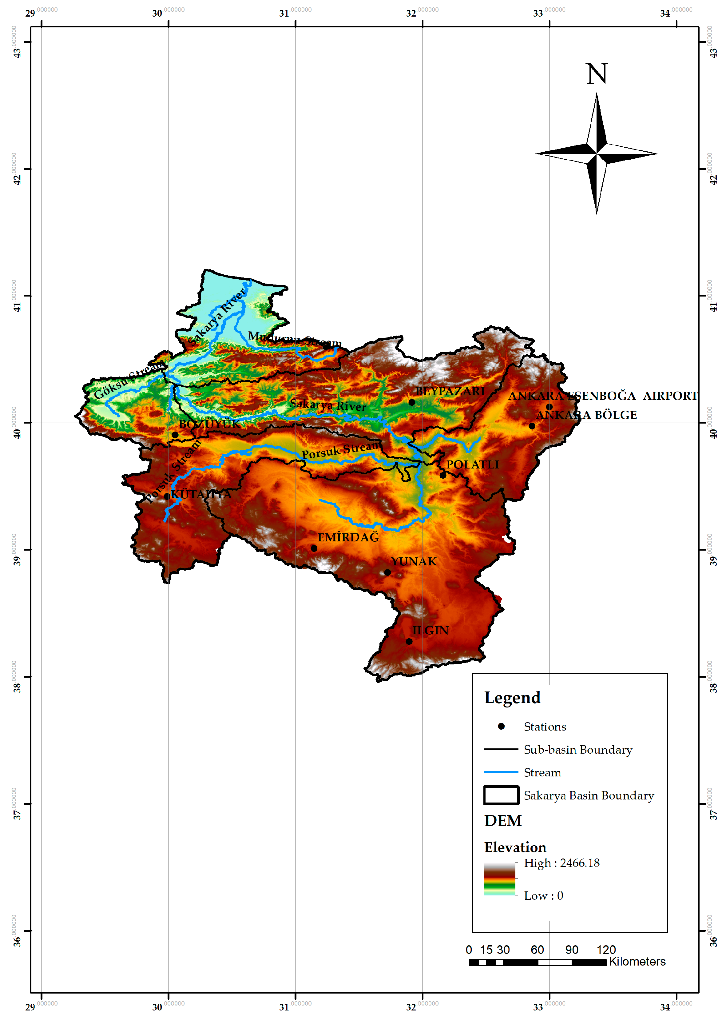
2.1. Study Region

Sakarya Basin, one of the 25 river basins in Türkiye, is located in the northwest of the country. It neighbors the Marmara and Eastern Black Sea Basins in the north, the Akarçay and Konya Closed Basins in the south, the Susurluk Basin in the west, and the Kızılırmak Basin in the east. The total basin area is 58,160 km² and is located between 37°96′–41°20′ northern latitudes and 29°26′–33°24′ eastern longitudes. In the basin, whose mean elevation is 965 m, the mean annual precipitation is 479 mm, and the mean annual temperature is 10.6 °C. Due to its location and the size of the area it covers, the Black Sea climate is observed in the north of the basin, while the Mediterranean climate is seen in the parts close to the Marmara Basin. A continental climate prevails in the middle of the basin, where summers are hot and winters are cold [46].

The monthly total precipitation data between 1991 and 2023 used in the meteorological drought analysis for the Sakarya Basin were taken from the General Directorate of Meteorology (MGM) for the nine meteorological observation stations. The information and the locations of these stations are given in

Table 1. Information on meteorological stations determined for drought analysis of Sakarya Basin.

Station	Station Number	Latitude	Longitude	Mean Annual Precipitation (mm)
Ankara Bölge	17130	39.9727	32.8637	412.36
Ankara Esenboğa Airport	17128	40.1240	32.9992	400.14
Beypazarı	17680	40.1608	31.9172	406.33
Bozüyük	17702	39.9039	30.0525	497.03
Emirdağ	17752	39.0098	31.1463	429.52
Ilgın	17832	38.2763	31.8940	435.32
Kütahya	17155	39.4171	29.9891	555.30
Polatlı	17728	39.5834	32.1624	362.12
Yunak	17798	38.8205	31.7258	441.05

and Figure 1, respectively.

The main river branch of the basin is the Sakarya River, fed by the Porsuk, Ankara, Karasu, Göksu, Çarksuyu, and Mudurnu Streams. The basin is divided into 6 sub-basins: Upper Sakarya, Porsuk Stream, Ankara Stream, Middle Sakarya, Göksu–Karasu, and Lower Sakarya Sub-basins, considering the hydrological, geological, and topographic situation. The largest lake in the basin is Sapanca Lake, and it meets the drinking and utility water needs of Sakarya province, where the population density is high [47].

2.2. Methods

2.2.1. Standardized Precipitation Index

Standardized precipitation index (SPI) is generally used to evaluate meteorological drought. SPI, which involves adapting a probability density function such as gamma or normal distribution to total precipitation amounts, allows dimensionless standard series to be obtained by Equation (1).

$$SPI={\displaystyle \frac{X-\overline{X}}{\sigma }}$$

(1)

Here $X$, $\overline{X}$, and $\sigma$ represent precipitation height (mm), mean precipitation, and standard deviation, respectively.

After the precipitation-probability relationship is established from historical records, the probability of any observed precipitation data and their deviation from the normal distribution, which has a mean of zero and a standard deviation of one, can be calculated. Situations where the SPI value is below zero are considered to be periods of drought, while situations when it rises above zero are considered to be periods where the drought is over, that is, rainy periods. In the SPI method, precipitation data are arranged for an uninterrupted period of at least 30 years.

Table 2. Drought categories according to SPI values [14].

SPI	Drought Categories
0 to −0.99	Mild drought
−1.0 to −1.49	Moderate drought
−1.5 to −1.99	Severe drought
$\le$−2.0	Extreme drought

gives drought severity categories according to SPI values [14].

2.2.2. Long Short-Term Memories

Long short-term memory (LSTM) is a novel recurrent network architecture (RNN) combined with a gradient-based learning algorithm designed to overcome error backflow issues in modeling time series. LSTM has a long-term dependency that makes it more accurate than traditional RNNs and uses it for future predictions [48]. In LSTM and RNNs, which are very similar to each other, the output of the previous step is used as the input of the current step and is kept in memory for a short time. Since RNNs cannot retain information for long, some information may be lost at the beginning of the network. Moreover, RNNs experience the problem of gradient extinction during backpropagation. To overcome these problems, gates that regulate and control the information flow are created in LSTM networks. Among these gates, the input gate takes the previous hidden state and the current input and applies it to the sigmoid function to update the cell state. The cell state allows for the retention or forgetting of information with the help of other gates. While the output gate gives the output of the cell, the forget gate decides the parts of the information to be forgotten and kept in memory [49]. The cell state updated according to the outputs from the gates can be represented mathematically by Equations (2)–(6):

$$f_t=\sigma \left(W_f\left[h_{t-1},x_t\right]+b_f\right)$$

(2)

$$i_t=\sigma \left(W_i\left[h_{t-1},x_t\right]+b_i\right)$$

(3)

$$c_t=\tanh (W_c[h_{t-1},x_t]+b_c$$

(4)

$$o_t=\sigma \left(W_o\left[h_{t-1},x_t\right]+b_o\right)$$

(5)

$$h_t=o_t\mathit{tan}h\left(c_t\right)$$

(6)

Here, $f_t$, $i_t$, and $o_t$ represent the forget gate vector, input gate vector, and output gate vector at step t, respectively; $c_t$ is the cell state vector at step t; $h_t$ and $h_{t-1}$ are the hidden state vectors known as output vectors at steps t and t − 1; $\sigma$ and $\mathrm{t}\mathrm{a}\mathrm{n}\mathrm{h}$ represent sigmoid and hyperbolic tangent functions; $W_f$ and $b_f$ are the weight matrix and bias of the forget gate; $W_i$ and $b_i$ are the weight matrix and bias of the input gate; $W_c$ and $b_c$ are the weight matrix and bias of the cell state; and $W_o$ and $b_o$ indicate the weight matrix and deviation of the output gate [50]. This given process continues repeatedly. Weight matrices ($W$) and deviation values ($b$) are learned by the model so that the difference between the real training values and LSTM output values is minimal [51].

2.2.3. Adaptive Moment Estimation Optimizer

The adaptive moment estimation (ADAM) optimizer, proposed by Kingma and Ba (2014), is a gradient-based optimization algorithm [52]. The method has a simple application, requires less memory, and is suitable for solving multi-data and multi-parameter problems. The algorithm optimizes the weights at each level [53]. It uses estimates of the first and second gradient moments that are known as the mean and variance by varying the learning rate for each weight in the neural network. For this reason, it is known as adaptive moment estimation [54]. The update rule of the ADAM optimizer can be shown by Equations (7) and (8):

$$m_t={\beta }_1{m}_{t-1}+(1-{\beta }_1)g_t$$

(7)

$$v_t={\beta }_2{v}_{t-1}+(1-{\beta }_2)g_t^2$$

(8)

where m and v are the moving averages, g is the gradient in the current batch, t is the number of iterations, and β₁ and β₂ are the hyperparameters. Then, the wanted values are obtained from the expected values with the bias-corrected estimators $\widehat{m_t}$ (and $\widehat{v_t}$) given in Equations (9) and (10).

$$\widehat{m_t}={\displaystyle \frac{m_t}{1-{\beta }_1^t}}$$

(9)

$$\widehat{v_t}={\displaystyle \frac{v_t}{1-{\beta }_2^t}}$$

(10)

The algorithm is concluded by scaling the learning rate separately for each parameter, and the weight update is performed using Equation (11).

$$w_t=w_{t-1}-\alpha {\displaystyle \frac{\widehat{m_t}}{ϵ+\sqrt{\widehat{v_t}}}}$$

(11)

where w is the model weight, α is the learning rate, t is the number of iterations, and ε is the default value of 10−8 to avoid division by zero [55].

2.2.4. Inverse Distance Weighting

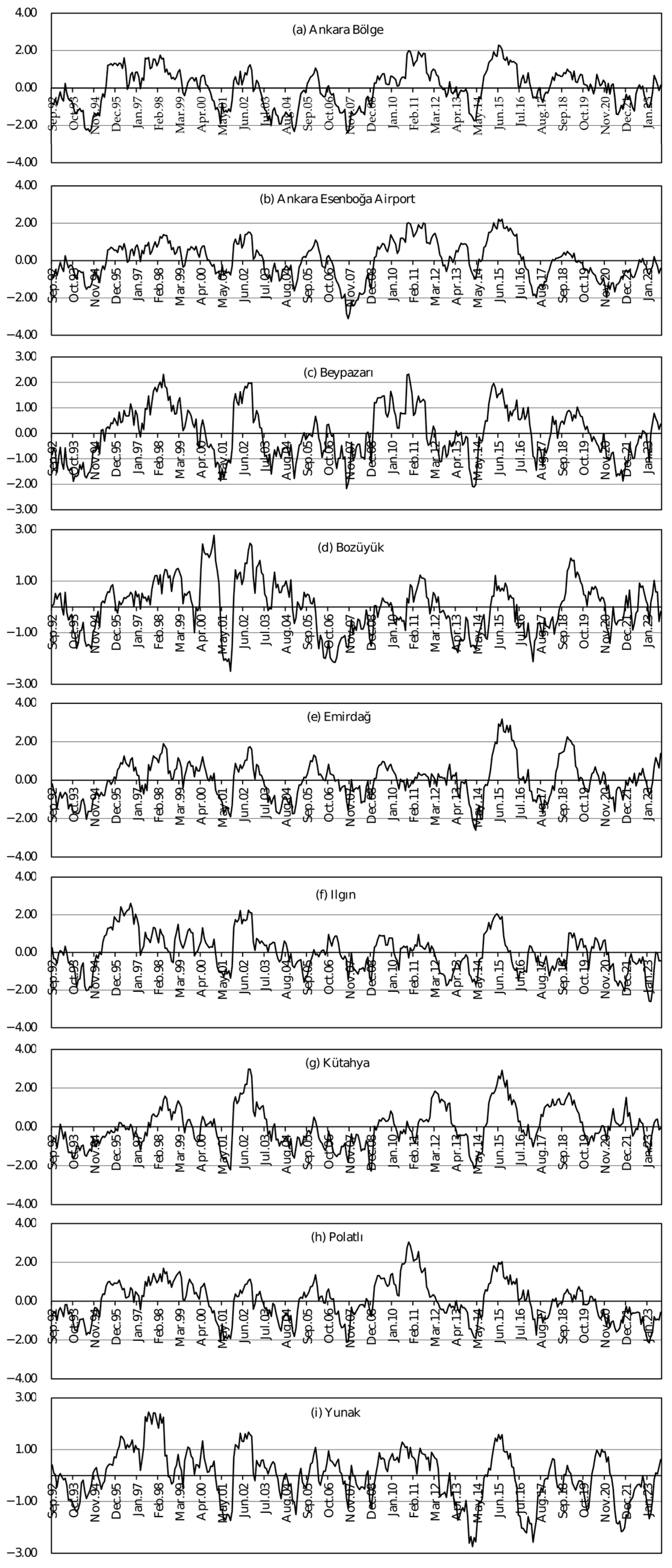
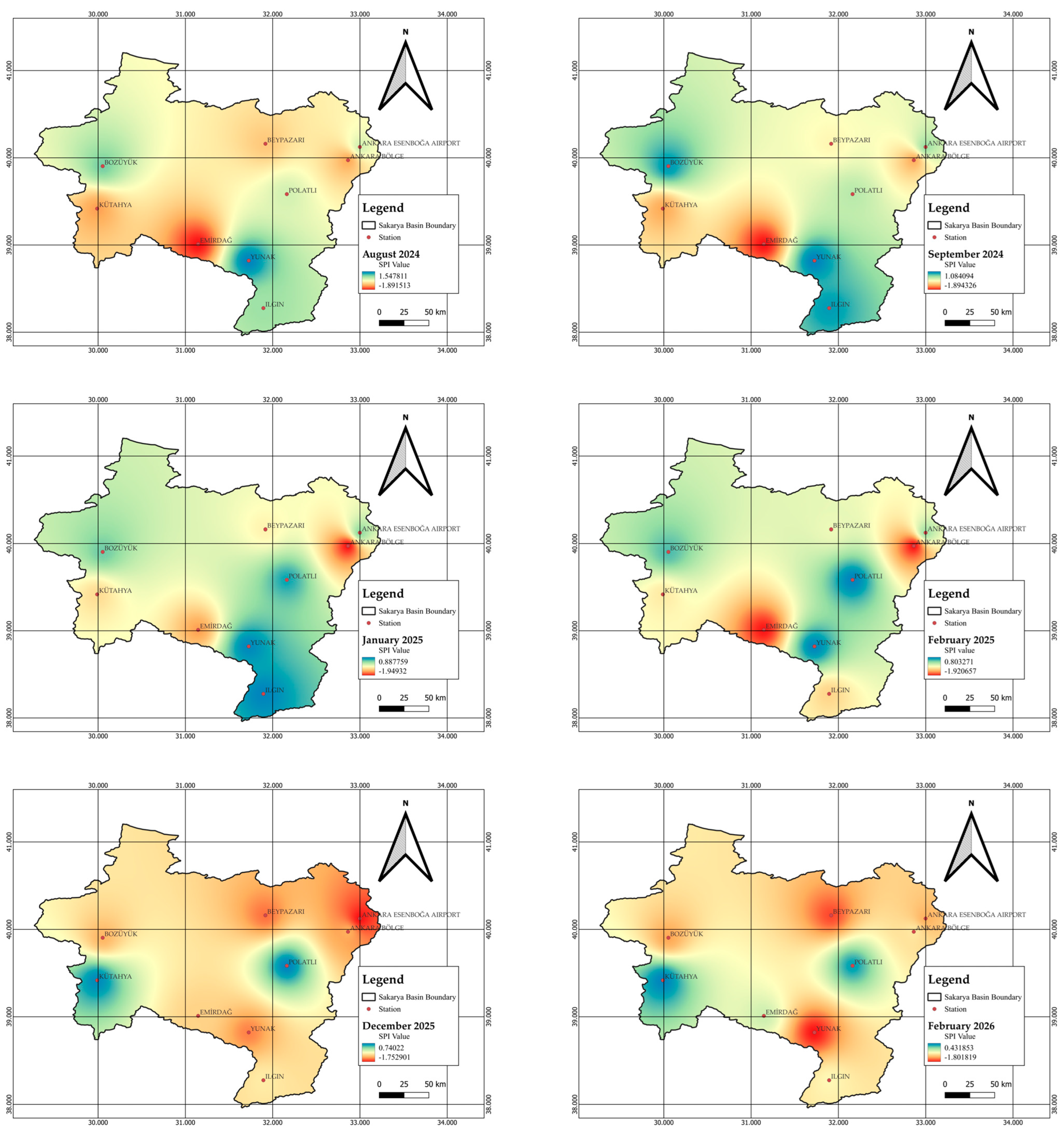
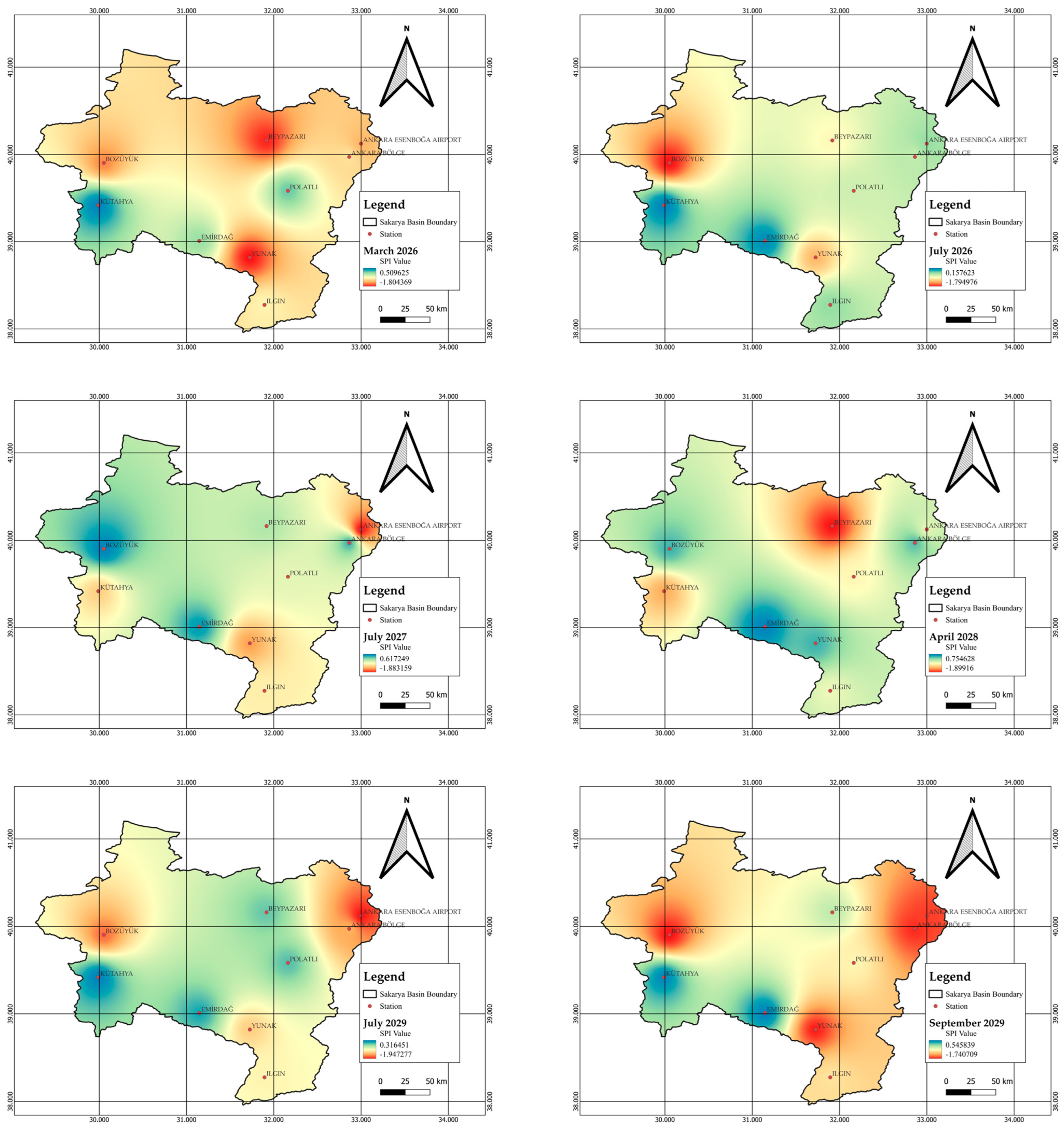
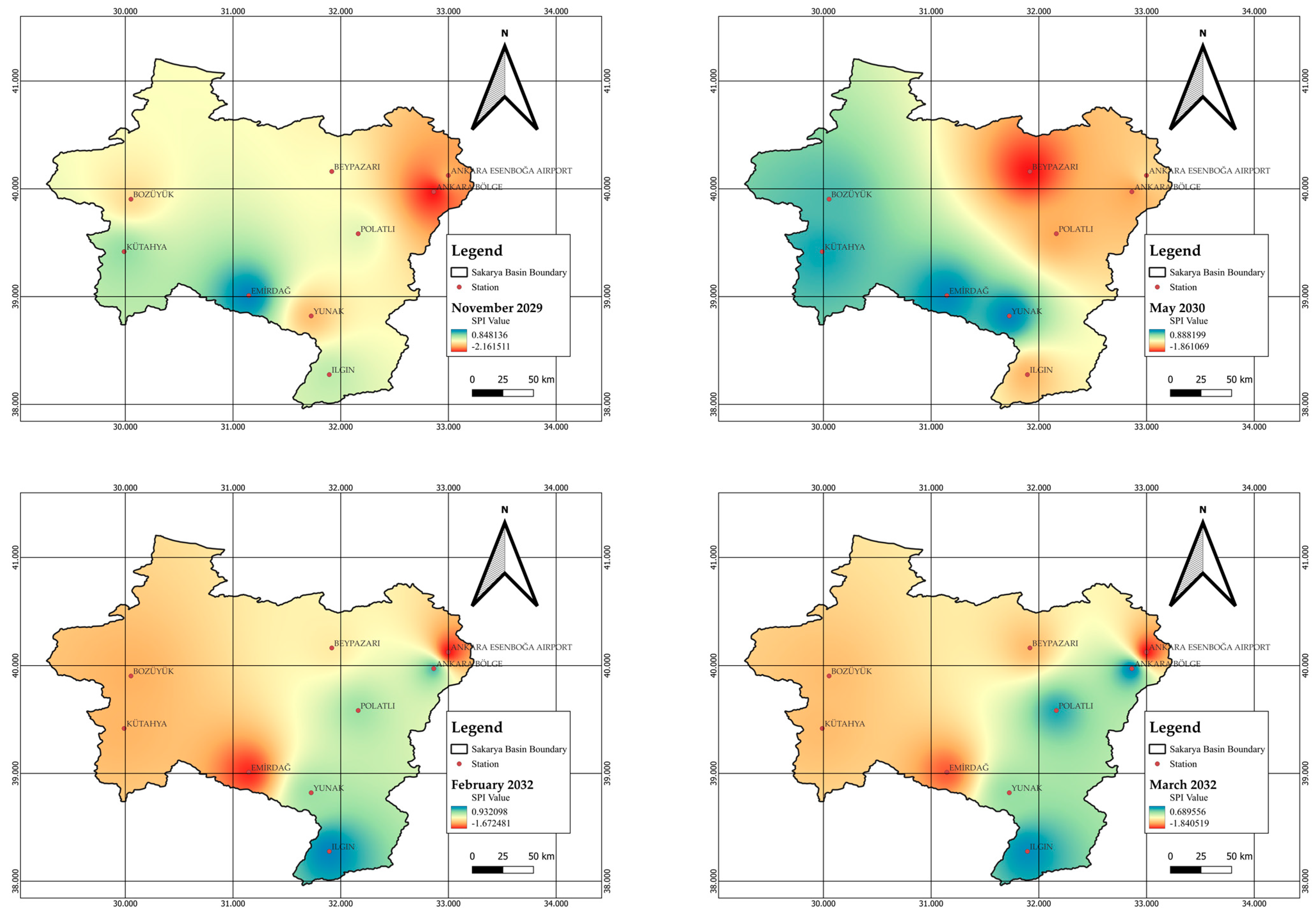
Inverse distance weighting (IDW) is an interpolation technique used to determine cell values of unsampled points by using sample points with known values. Predicted values are a function of the distance and size of nearby points. Increasing the distance causes the effect on the cell to be predicted to decrease. In this method, which is a deterministic approach, properties such as general distribution, trend, anisotropy, and data clustering are examined [56]. Generally, a weighted moving average is used for interpolation. Prediction is made with IDW, an intermediate value generator, as follows [57,58]:

$$\theta \left(X_0\right)={\sum }_{i=1}^n{\displaystyle \frac{\theta \left(X_i\right)d_i^{-r}}{{\sum }_{i=1}^n{d}_i^{-r}}}$$

(12)

where $\theta \left(X_0\right)$ is the interpolated value at the unsampled location $X_0$ based on observed values of $\theta \left(X_i\right)$ at surrounding locations up to i = 1, 2, …, n. $d_i$ is the distance between the unknown and observed values, and r is the power parameter of the appropriate constant. As r grows, the assigned weight of observations at a greater distance from the location of the forecast becomes smaller. Using Equation (12), unknown values were calculated, and maps were produced in the ARCGIS (v10.8) environment, which is a GIS software.

3. Results

This study aims to predict the times and locations of future meteorological droughts in Sakarya Basin in Türkiye. Short timescale SPI values such as those at 3 and 6 months are more effective in identifying short-term droughts, while 12-month timescale SPI values are better for identifying less frequent longer-term drought events [29,59]. Thus, to determine meteorological drought values in this study, 12-month timescale SPI series were calculated using precipitation values obtained from the Ankara Bölge, Ankara Esenboğa Airport, Beypazarı, Bozüyük, Emirdağ, Ilgın, Kütahya, Polatlı, and Yunak stations in the basin. The 12-month timescale SPI series of these stations are given in Figure 2. As seen from Figure 2, dry and rainy periods occurred at almost the same time intervals at all stations.

Since the use of linear statistical methods in predicting non-linear time series is insufficient due to data complexity, the use of LSTM, one of the deep neural network algorithms, is frequently preferred [60,61]. Hence, the SPI series, which were time series, were modeled using LSTM to predict possible droughts in the future. Before proceeding to the modeling, the stationarity of the SPI series of each station was checked. For this purpose, ADF, one of Dickey–Fuller’s parametric unit root tests, was used. The statistics obtained by the ADF test are given in

Table 3. ADF test results.

Station	ADF Statistics	p-Value	Critical Value (1%)	Critical Value (5%)	Critical Value (10%)
Ankara Bölge	−3.681	0.0240	−3.984	−3.423	−3.134
Ankara Esenboğa Airport	−3.490	0.0400	−3.984	−3.423	−3.134
Beypazarı	−3.593	0.0300	−3.984	−3.423	−3.134
Bozüyük	−3.651	0.0260	−3.984	−3.423	−3.134
Emirdağ	−4.866	0.0003	−3.984	−3.423	−3.134
Ilgın	−4.311	0.0030	−3.984	−3.423	−3.134
Kütahya	−4.390	0.0023	−3.984	−3.423	−3.134
Polatlı	−3.420	0.0488	−3.984	−3.423	−3.134
Yunak	−4.432	0.0019	−3.984	−3.423	−3.134

.

In order for the SPI series to meet the stationarity condition, the p-value must be below 0.05 and the absolute value of the test statistic must be greater than the absolute value of the 5% critical value.

In the modeling stage, the SPI series that may occur in the next 10 years (2024–2034) at the Ankara Region, Ankara Esenboğa Airport, Beypazarı, Bozüyük, Emirdağ, Ilgın, Kütahya, Polatlı, and Yunak stations were forecasted using LSTM. The first 80% of the monthly data between 1991 and 2023 were used for training, and the last 20% were used for testing to define better periodicity. The performance of LSTM models was assessed using mean squared error (MSE) as described in Equation (13):

$$MSE={\displaystyle \frac{1}{N}}{\sum }_{i=1}^N{(X_{ireal}-X_{iforecast})}^2$$

(13)

where N is the number of real data, and $X_{ireal}$ and $X_{iforecast}$ are SPI values and LSTM model results, respectively.

This study focused on forecasting future SPI series and employed the PyTorch library within a Python (v3.12) environment in the LSTM method. Loshchilov and Hutter (2016) said that future SPI series also reflected periodicity with correlograms like the historical series with the CosineAnnealingLR as an LR strategy added to the LSTM torch [62]. Therefore, CosineAnnealingLR was used to obtain periodicity close to the historical series in the future 10-year series in this study. The various hyperparameters were explored to identify the optimal model configuration. The optimal model configuration is given in

Table 4. Optimal model configuration for all stations.

Station	Hidden Layer Size	Number of Hidden Layers
Emirdağ	128	3
Yunak	128	3
Ankara Region	256	3
Ankara Esenboğa Airport	256	2
Beypazarı	256	2
Kütahya	256	5
Polatlı	256	3
Bozüyük	512	3
Ilgın	512	3

. Moreover, hyperparameter tunings of the methodology and findings are as follows:

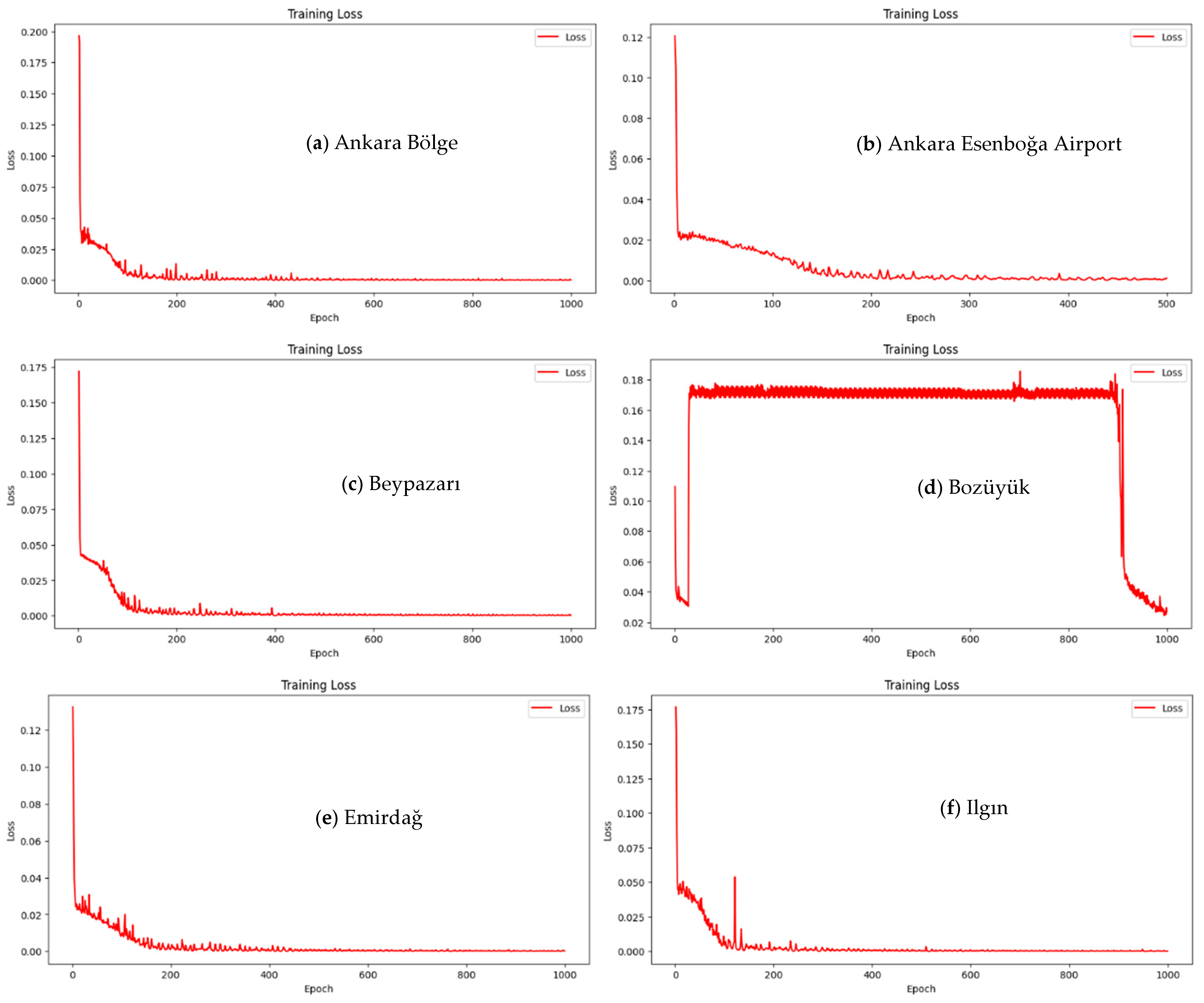
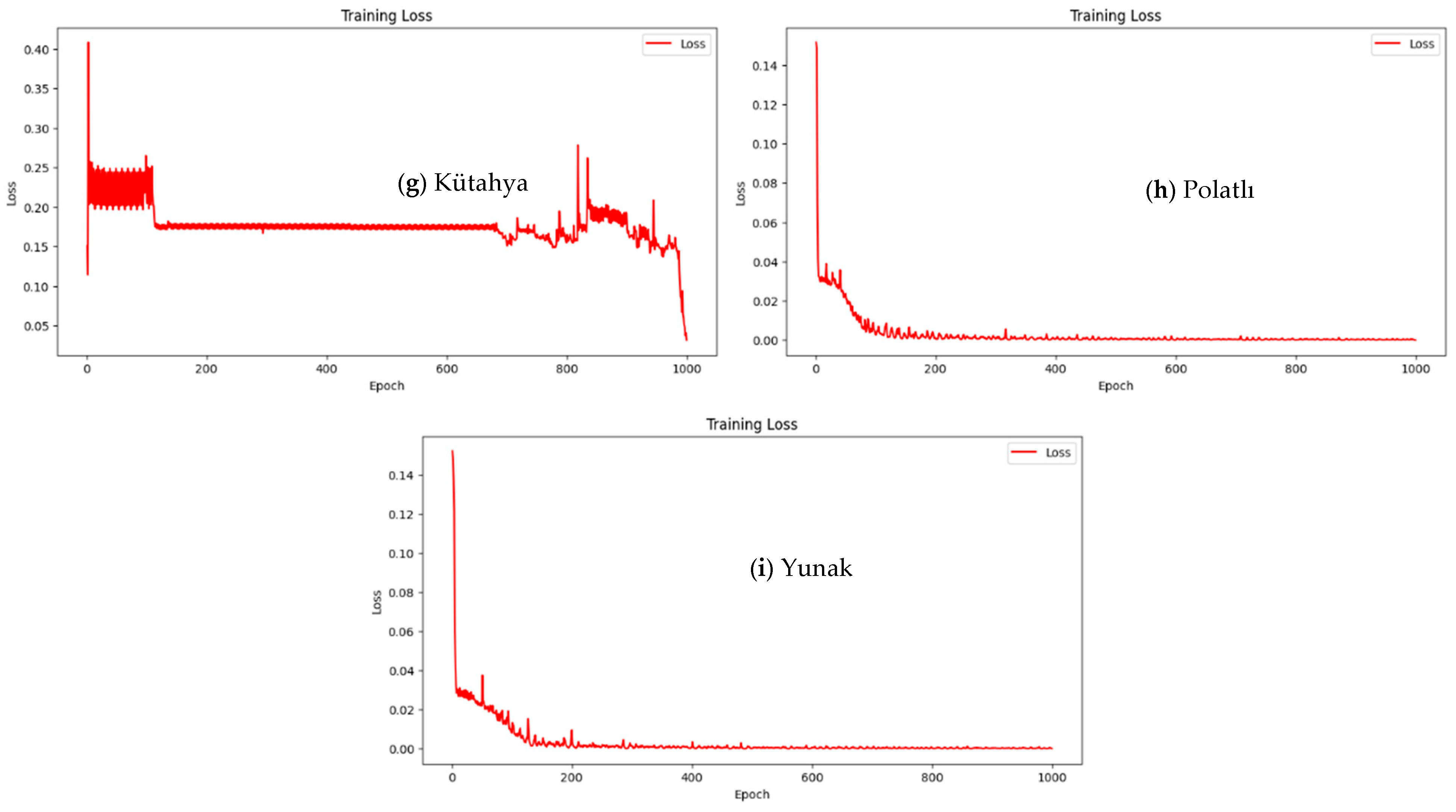
• Learning Rate: It was set to 0.001 in all models.
• Epoch Range: Models were trained for 500 to 1000 epochs to minimize MSE towards zero.
• Hidden Layer Sizes: Considered sizes were 32, 64, 128, 256, and 512.
• Number of Hidden Layers (Nodes): Models were tested with 1, 2, 3, 4, and 5 hidden layers.
• Optimizer: The Adam optimizer was utilized in all cases.

It was observed that the MSE value decreased (losses) with the increase in the number of epochs during the training phase at all stations in Figure 3. An epoch refers to each iteration during model training in which the model uses the entire training set to update its weights. This indicates that the predictions of the model are getting closer to the true values as training progresses. A decrease in the MSE over epochs indicates that the model is improving its accuracy by adjusting its weights through backpropagation and gradient descent. If the MSE continues to decrease and then remains constant, it means that the model is learning underlying patterns in the training data.

Historical and forecasted SPI values for the future 10-year time series and trend line equations are given in Figure 4. When Figure 4 is examined, the similar trends were obtained for historical and forecasted SPI values. The SPI series for the next 10 years covering the years 2024–2034 obtained from the LSTM models for all stations follow a similar pattern to the past SPI series, indicating that the models can project historical climatic or meteorological conditions into the future, continuing increasing or decreasing trends. At the same time, similar seasonal patterns are formed in the past and future series.

In addition, the correlograms were compared to evaluate the compatibility of the historical and forecasted SPI series. Figure 5 shows the autocorrelation functions (ACFs) of the historical and forecasted SPI series for each station, and it was observed that the ACFs of the forecasted SPI series were similar to the ACFs of the historical SPI series. ACFs, which show how much a time series is related to its own historical values, measure this relationship with a certain number of lags. According to the lag axis, it shows how long the time series is related to itself. ACF values that start from a high value and gradually decrease show the mean of time series changes over time. From here, it can also be said that the time series has an increasing or decreasing trend. In the Ankara Region, Ankara Esenboğa Airport, Bozüyük, Emirdağ, Ilgın, Kütahya, Polatlı and Yunak stations, the ACFs of the historical and forecasted SPI series remain outside the 95% confidence interval at lags of up to 5 to 7 months. From here, it is understood once again that the forecasted SPI series have a similar trend to the historical SPI series. At Beypazarı station, the increasing trend of the historical series was caught with a lag of up to 3 months. ACFs of future time series at 95% confidence interval for all stations show that the model successfully captures correlations in historical data.

4. Discussion

In this study, SPI and LSTM models were used to forecast future drought conditions in the Sakarya Basin. The main objective of the study is to forecast drought risk maps that may occur in the nine meteorological stations between 2024 and 2034. The drought maps created are of critical importance for water resource management and planning in the region and will help make strategic decisions to minimize possible drought effects. For this purpose, time series of SPI values of all stations for the next 10 years were created in order to select the most severe drought values that may occur in the future (Figure 6).

It can be seen from Figure 6a, in which the next 10-year SPI series is presented for all stations, the forecasted SPI series of the Ankara Bölge and Ankara Esenboğa Airport stations frequently reach positive values, indicating rainy periods. However, SPI values below −2 indicate extreme drought, and above 2 indicate extreme rainy durations. The graph shows the most severe dry times likely to occur in the region, and drought periods close to −2 are also observed at the Ankara Bölge, Ankara Esenboğa Airport, Beypazarı, and Emirdağ stations. The Yunak and Bozüyük stations reached positive SPI values, especially Yunak station, which frequently exceeded 1, indicating rainy periods. According to Figure 6, the most serious droughts in the future will occur on the following dates, respectively: August and September 2024; January, February, and December 2025; February, March, and July 2026; July 2027; April 2028; July, September, and November 2029; May 2030; February, March, June, and October 2032; and January 2033. Additionally, Figure 6b is given as a 100% stacked line graph to compare the effect of the forecasted SPI values for each station on the general drought in the region as a percentage. That is, Figure 6b is a graph of the change in the anomalies of the percentage SPI values in the future for all stations over time. The SPI values expressed in percentages show how much the SPI value of each station has increased or decreased compared to the long-term mean of the region. The Ankara Bölge and Ankara Esenboğa Airport stations show similar trends and have the smallest extreme drought values compared to other stations. Yunak station has remarkable peaks, especially in terms of positive anomalies. This shows that much more precipitation than the regional mean can be expected in Yunak during some periods.

Since the drought has spatial and temporal variations, drought maps for the Sakarya Basin were created using the IDW interpolation technique available in the ARCGIS(v10.8) package. The IDW technique assumes that points closer to stations have higher potential than points further away. The forecasted SPI values of nine meteorological stations for the period from 2024 to 2034 were interpolated for the driest months in Figure 6. Figure 7 shows local changes in drought for August and September 2024; January, February, and December 2025; February, March, and July 2026; July 2027; April 2028; July, September, and November 2029; May 2030; February, March, June, and October 2032; and January 2033 when the riskiest droughts are expected in the future.

According to the future drought maps given in Figure 7, consistent spatial distributions were obtained. According to the color scale used in the maps, blue and its shades indicate areas with rain, yellow represents areas with a mild risk of drought, orange indicates areas with a moderate risk of drought, and dark orange denotes areas with a severe risk of drought. Extreme drought is shown in red. It has been observed that the drought value in the region will range from 1.54 to −2.16 in the future. Generally, drought is estimated to occur in the severe drought category between −1.70 and −1.90, occurring in moderate drought levels. While a consistent spatial distribution is usually obtained in the region for the four drought categories, extreme drought is predicted to happen in the north and east of the region, at the Ankara Esenboğa airport and Ankara Regional stations especially. It could be said that mild drought and moderate drought categories are expected to occur in the central and western parts of the region, and it is inevitable that drought will occur in the future around the Emirdağ and Yunak stations located in the south of the region. It is forecasted that there will be rainy periods around the Ilgın station in the south of the region. Drought affecting a large part of the region is expected, especially in December 2025, February 2026, September 2029, and June 2032.

5. Conclusions

In this study, analyses performed using the LSTM method to forecast future drought conditions in the Sakarya Basin, Türkiye, have revealed important findings for the water resource management and planning of the region. Future SPI values for the period between 2024 and 2034 were forecasted with the LSTM model using SPI series calculated based on monthly precipitation data between 1991 and 2023.

Future drought times were effectively forecasted with LSTM models that have the ability to process complex and non-linear time series data. The suitability of the model was demonstrated by the similarity of historical and forecasted SPI values. The forecasted SPI series followed past drought patterns and showed that similar trends will continue in the future. In particular, severe droughts that will occur during certain periods and the spatial distribution of these droughts provide critical information for regional water management. The drought maps created using the IDW interpolation technique determined the areas with the highest drought risk in the region. The findings of the study provide a scientific basis for the development of water resource management, agriculture, and disaster preparedness strategies in the region. The predictions of the timing and severity of future droughts will enable authorities and stakeholders to take precautions.

It is aimed to improve the results by using new LSTM models in the future. The study is based on datasets of nine stations from Sakarya Basin. Having more than nine stations at the high and low elevation points of the basin may eliminate the limitation of the study. Including more stations distributed throughout the basin may increase the generalizability of the results. More stations allow for more frequent data collection in different parts of the basin. This increases spatial resolution and can more accurately reflect regional differences. In particular, precipitation and SPI changes in topographically complex regions can be better modeled. At the same time, increasing the number of stations increases the accuracy of spatial interpolation techniques. The interpolation methods such as IDW can provide more precise results with more data points. Thus, future drought forecasting errors can be reduced for regions with sparse station networks and more reliable drought maps can be created. Moreover, using different optimization methods for future studies may improve the performance of the LSTM model. In the study, SPI series obtained from precipitation data were used for drought analysis. However, different hydrological parameters (such as streamflow, evapotranspiration), atmospheric parameters (such as air temperature, humidity, wind speed, pressure), and parameters related to human activities (such as the greenhouse gas effect) can also be used in drought analysis. Global warming effects, such as temperature changes and greenhouse gas emissions, can cause soil moisture depletion and agricultural drought while increasing surface runoff. In future studies, future drought forecasting of the region can be made by working with different drought indices using these and similar variables.

In conclusion, this study has made significant progress in forecasting future meteorological droughts in the Sakarya Basin. The future predictions made using the LSTM model provide an important tool for improving water resource management and making decisions to solve water scarcity problems that may occur in the region.

References

1. Türkeş, M. A Detailed Analysis of the Drought, Desertification and the United Nations Convention to Combat Desertification. Marmara J. Eur. Stud. 2012, 20, 7–55. [Google Scholar] [CrossRef]
2. Ozcelik, C.; Yilmaz, M.U.; Benli, K. Assessing drought in Turkish basins through satellite observations. Int. J. Climatol. 2024, 44, 3613–3640. [Google Scholar] [CrossRef]
3. Serkendiz, H.; Tatli, H.; Kılıç, A.; Çetin, M.; Sungur, A. Analysis of drought intensity, frequency and trends using the spei in Turkey. Theor. Appl. Climatol. 2024, 155, 2997–3012. [Google Scholar] [CrossRef]
4. Korkmaz, M.; Kuriqi, A. Regional Climate Change and Drought Dynamics in Tunceli, Turkey: Insights from Drought Indices. Water Conserv. Sci. Eng. 2024, 9, 49. [Google Scholar] [CrossRef]
5. Turan, E.S. Turkey’s Drought Status Associated with Climate Change. J. Nat. Hazards Environ. 2018, 4, 63–69. [Google Scholar] [CrossRef]
6. Ballar, Z. Stormwater Management in Cities as a Climate Change Adaptation Strategy: Case of Halkapınar District (Izmir, Turkey). Master’s Thesis, Izmir Institute of Technology, Urla, Turkey, 2019. [Google Scholar]
7. Kadıoğlu, M.; Ünal, Y.; İlhan, A.; Yürük, C. Climate Change and Sustainability in Agriculture in Turkey. Federation of Turkish Food and Beverage Industry Associations. 2017. Available online: https://www.tgdf.org.tr/wp-content/uploads/2017/10/iklim-degisikligi-rapor-elma.compressed.pdf (accessed on 11 July 2024).
8. Türkeş, M.; Sümer, U.M. Spatial and Temporal Patterns of Trends and Variability in Diurnal Temperature Ranges of Turkey. Theor. Appl. Climatol. 2004, 77, 195–227. [Google Scholar] [CrossRef]
9. Türkeş, M. Observed and Projected Climate Change, Drought and Desertification in Turkey. Ankara Univ. J. Environ. Sci. 2012, 4, 1–32. [Google Scholar] [CrossRef]
10. Yüksel, G.; Sökün, H. Drought Analysis with Dynamic Mode Decomposition for the Aegean Region. Int. J. 3D Print. Technol. Digit. Ind. 2022, 6, 54–61. [Google Scholar] [CrossRef]
11. Wei, X.; Huang, S.; Liu, D.; Li, J.; Huang, Q.; Leng, G.; Shi, H.; Peng, J. The response of agricultural drought to meteorological drought modulated by air temperature. J. Hydrol. 2024, 639, 131626. [Google Scholar] [CrossRef]
12. Wang, Z.; Chang, J.; Wang, Y.; Yang, Y.; Guo, Y.; Yang, G.; He, B. Temporal and spatial propagation characteristics of meteorological drought to hydrological drought and influencing factors. Atmos. Res. 2024, 299, 107212. [Google Scholar] [CrossRef]
13. Arra, A.A.; Alashan, S.; Şişman, E. Trends of meteorological and hydrological droughts and associated parameters using innovative approaches. J. Hydrol. 2024, 640, 131661. [Google Scholar] [CrossRef]
14. McKee, T.B.; Doesken, N.J.; Kleist, J. The Relationship of Drought Frequency and Duration to Time Scales. In Proceedings of the 8th Conference on Applied Climatology, Anaheim, CA, USA, 17–22 January 1993; pp. 179–183. [Google Scholar]
15. Oluwatobi, A.; Gbenga, O.; Oluwafunbi, F. An Artificial Intelligence Based Drought Predictions in Part of the Tropics. J. Urban Environ. Eng. 2017, 11, 165–173. [Google Scholar] [CrossRef]
16. El Ibrahimi, A.; Baali, A. Application of Several Artificial Intelligence Models for Forecasting Meteorological Drought Using the Standardized Precipitation Index in the Saïss Plain (Northern Morocco). Int. J. Intell. Eng. Syst. 2018, 11, 267–275. [Google Scholar] [CrossRef]
17. Malik, A.; Kumar, A.; Rai, P.; Kuriqi, A. Prediction of Multi-Scalar Standardized Precipitation Index by Using Artificial Intelligence and Regression Models. Climate 2021, 9, 28. [Google Scholar] [CrossRef]
18. Moreira, E.E.; Paulo, A.A.; Pereira, L.S.; Mexia, J.T. Analysis of SPI Drought Class Transitions Using Loglinear Models. J. Hydrol. 2006, 331, 349–359. [Google Scholar] [CrossRef]
19. Šebenik, U.; Brilly, M.; Šraj, M. Drought Analysis Using the Standardized Precipitation Index (SPI). Acta Geogr. Slov. 2017, 57, 31–49. [Google Scholar] [CrossRef]
20. Bhunia, P.; Das, P.; Maiti, R. Meteorological Drought Study through SPI in Three Drought Prone Districts of West Bengal, India. Earth Syst. Environ. 2020, 4, 43–55. [Google Scholar] [CrossRef]
21. Wi, S.; Steinschneider, S. On the need for physical constraints in deep learning rainfall–runoff projections under climate change: A sensitivity analysis to warming and shifts in potential evapotranspiration. Hydrol. Earth Syst. Sci. 2024, 28, 479–503. [Google Scholar] [CrossRef]
22. Jeon, S.; Kim, J. Artificial intelligence to predict climate and weather change. JMST Adv. 2024, 6, 67–73. [Google Scholar] [CrossRef]
23. Swagatika, S.; Paul, J.C.; Sahoo, B.B.; Gupta, S.K.; Singh, P.K. Improving the forecasting accuracy of monthly runoff time series of the Brahmani River in India using a hybrid deep learning model. J. Water Clim. Chang. 2024, 15, 139–156. [Google Scholar] [CrossRef]
24. Renteria-Mena, J.B.; Plaza, D.; Giraldo, E. Multivariate Hydrological Modeling Based on Long Short-Term Memory Networks for Water Level Forecasting. Information 2024, 15, 358. [Google Scholar] [CrossRef]
25. Lu, M.; Xu, X. TRNN: An efficient time-series recurrent neural network for stock price prediction. Inf. Sci. 2024, 657, 119951. [Google Scholar] [CrossRef]
26. Dikshit, A.; Pradhan, B.; Alamri, A.M. Long Lead Time Drought Forecasting Using Lagged Climate Variables and a Stacked Long Short-Term Memory Model. Sci. Total Environ. 2021, 755, 142638. [Google Scholar] [CrossRef] [PubMed]
27. Danandeh Mehr, A.; Rikhtehgar Ghiasi, A.; Yaseen, Z.M.; Sorman, A.U.; Abualigah, L. A Novel Intelligent Deep Learning Predictive Model for Meteorological Drought Forecasting. J. Ambient Intell. Humaniz. Comput. 2022, 14, 10441–10455. [Google Scholar] [CrossRef]
28. Duong, T.A.; Bui, M.D.; Rutschmann, P. Long Short Term Memory for Monthly Rainfall Prediction in Camau, Vietnam. Res. Gate 2018. in preprint. [Google Scholar]
29. Poornima, S.; Pushpalatha, M. Drought Prediction Based on SPI and SPEI with Varying Timescales Using LSTM Recurrent Neural Network. Soft Comput. 2019, 23, 8399–8412. [Google Scholar] [CrossRef]
30. Samad, A.; Gautam, V.; Jain, P.; Sarkar, K. An Approach for Rainfall Prediction Using Long Short Term Memory Neural Network. In Proceedings of the 2020 IEEE 5th International Conference on Computing Communication and Automation (ICCCA), Greater Noida, India, 30–31 October 2020; pp. 190–195. [Google Scholar]
31. Xu, D.; Zhang, Q.; Ding, Y.; Zhang, D. Application of a Hybrid ARIMA-LSTM Model Based on the SPEI for Drought Forecasting. Environ. Sci. Pollut. Res. 2022, 29, 4128–4144. [Google Scholar] [CrossRef]
32. Anh, D.T.; Thanh, D.V.; Le, H.M.; Sy, B.T.; Tanim, A.H.; Pham, Q.B.; Thanh, D.D.; Son, T.M.; Dang, N.M. Effect of Gradient Descent Optimizers and Dropout Technique on Deep Learning LSTM Performance in Rainfall-Runoff Modeling. Water Resour. Manag. 2023, 37, 639–657. [Google Scholar] [CrossRef]
33. Solgi, R.; Loaiciga, H.A.; Kram, M. Long Short-Term Memory Neural Network (LSTM-NN) for Aquifer Level Time Series Forecasting Using In-Situ Piezometric Observations. J. Hydrol. 2021, 601, 126800. [Google Scholar] [CrossRef]
34. Orieschnig, C.; Cavus, Y. Spatial characterization of drought through CHIRPS and a station-based dataset in the Eastern Mediterranean. Proc. IAHS 2024, 385, 79–84. [Google Scholar] [CrossRef]
35. Workneh, H.T.; Chen, X.; Ma, Y.; Bayable, E.; Dash, A. Comparison of IDW, Kriging and orographic based linear interpolations of rainfall in six rainfall regimes of Ethiopia. J. Hydrol. Reg. Stud. 2024, 52, 101696. [Google Scholar] [CrossRef]
36. Daly, C.; Neilson, R.P.; Phillips, D.L. A Statistical-Topographic Model for Mapping Climatological Precipitation over Mountainous Terrain. J. Appl. Meteorol. Climatol. 1994, 33, 140–158. [Google Scholar] [CrossRef]
37. Ali, M.G.; Younes, K.; Esmaeil, A.; Fatemeh, T. Assessment of Geostatistical Methods for Spatial Analysis of SPI and EDI Drought Indices. World Appl. Sci. J. 2011, 15, 474–482. [Google Scholar]
38. Goovaerts, P. Geostatistical Approaches for Incorporating Elevation into the Spatial Interpolation of Rainfall. J. Hydrol. 2000, 228, 113–129. [Google Scholar] [CrossRef]
39. Rahman, M.R.; Lateh, H. Meteorological Drought in Bangladesh: Assessing, Analysing and Hazard Mapping Using SPI, GIS and Monthly Rainfall Data. Environ. Earth Sci. 2016, 75, 1026. [Google Scholar] [CrossRef]
40. Mahajan, D.R.; Dodamani, B.M. Spatial and Temporal Drought Analysis in the Krishna River Basin of Maharashtra, India. Cogent Eng. 2016, 3, 1185926. [Google Scholar] [CrossRef]
41. Boustani, A.; Ülke, A. Investigation of Meteorological Drought Indices for Environmental Assessment of Yesilirmak Region. J. Environ. Treat. Tech. 2020, 8, 374–381. [Google Scholar]
42. Coşkun, Ö.; Citakoglu, H. Prediction of the Standardized Precipitation Index Based on the Long Short-Term Memory and Empirical Mode Decomposition-Extreme Learning Machine Models: The Case of Sakarya, Türkiye. Phys. Chem. Earth Parts A/B/C 2023, 131, 103418. [Google Scholar] [CrossRef]
43. Duvan, A.; Aktürk, G.; Yıldız, O. Effect of Climate Change on Spatiotemporal Characteristics of Meteorological Drought in Sakarya Basin, Turkey. J. Eng. Sci. Res. 2021, 3, 207–217. [Google Scholar] [CrossRef]
44. Varol, T.; Atesoglu, A.; Ozel, H.B.; Cetin, M. Copula-based multivariate standardized drought index (MSDI) and length, severity, and frequency of hydrological drought in the Upper Sakarya Basin, Turkey. Nat. Hazards 2023, 116, 3669–3683. [Google Scholar] [CrossRef]
45. Kartal, V.; Emiroglu, M.E. Hydrological Drought and Trend Analysis in Kızılırmak, Yeşilırmak and Sakarya Basins. Pure Appl. Geophys. 2024, 181, 1919–1943. [Google Scholar] [CrossRef]
46. TUBITAK. Watershed Protection Action Plan for Sakarya Basin, Final Report; TUBITAK: İstanbul, Turkey, 2013. [Google Scholar]
47. Yaykiran, S. Structuring the High Resolution Hydrological Model of Sakarya Basin. Master’s Thesis, Istanbul Technical University, İstanbul, Turkey, 2016. [Google Scholar]
48. Hochreiter, S.; Schmidhuber, J. Long Short-Term Memory. Neural Comput. 1997, 9, 1735–1780. [Google Scholar] [CrossRef] [PubMed]
49. Selvin, S.; Vinayakumar, R.; Gopalakrishnan, E.A.; Menon, V.K.; Soman, K.P. Stock Price Prediction Using LSTM, RNN and CNN-Sliding Window Model. In Proceedings of the 2017 International Conference on Advances in Computing, Communications and Informatics (ICACCI), Udupi, India, 13–16 September 2017; pp. 1643–1647. [Google Scholar]
50. Wu, X.; Zhou, J.; Yu, H.; Liu, D.; Xie, K.; Chen, Y.; Hu, J.; Sun, H.; Xing, F. The Development of a Hybrid Wavelet-ARIMA-LSTM Model for Precipitation Amounts and Drought Analysis. Atmosphere 2021, 12, 74. [Google Scholar] [CrossRef]
51. Sagheer, A.; Kotb, M. Time Series Forecasting of Petroleum Production Using Deep LSTM Recurrent Networks. Neurocomputing 2019, 323, 203–213. [Google Scholar] [CrossRef]
52. Kingma, D.P.; Ba, J.L. Adam: A Method for Stochastic Optimization. In Proceedings of the 3rd International Conference on Learning Representations, San Diego, CA, USA, 7–9 May 2015; pp. 1–15. [Google Scholar]
53. Chandriah, K.K.; Naraganahalli, R.V. RNN/LSTM with Modified Adam Optimizer in Deep Learning Approach for Automobile Spare Parts Demand Forecasting. Multimed. Tools Appl. 2021, 80, 26145–26159. [Google Scholar] [CrossRef]
54. Kumar, G.P.; Priya, G.S.; Dileep, M.; Raju, B.E.; Shaik, A.R.; Sarman, K.V.S.H.G. Image Deconvolution Using Deep Learning-Based Adam Optimizer. In Proceedings of the 2022 6th International Conference on Electronics, Communication and Aerospace Technology, Coimbatore, India, 1–3 December 2022; pp. 901–904. [Google Scholar]
55. Şen, S.Y.; Özkurt, N. Convolutional Neural Network Hyperparameter Tuning with Adam Optimizer for ECG Classification. In Proceedings of the 2020 Innovations in Intelligent Systems and Applications Conference (ASYU), Istanbul, Turkey, 15–17 October 2020; pp. 1–6. [Google Scholar]
56. Doğan, H.M.; Yılmaz, D.S.; Kılıç, O.M. Mapping and Interpreting Some Soil Surface Properties of Central Kelkit Basin by Inverse Distance Weighted (IDW) Method. Gaziosmanpaşa J. Sci. Res. 2013, 6, 46–54. [Google Scholar]
57. Lloyd, C.D. Local Models for Spatial Analysis; CRC Press: Boca Raton, FL, USA, 2010. [Google Scholar]
58. Chen, H.; Fan, L.; Wu, W.; Liu, H.B. Comparison of Spatial Interpolation Methods for Soil Moisture and Its Application for Monitoring Drought. Environ. Monit. Assess. 2017, 189, 525. [Google Scholar] [CrossRef] [PubMed]
59. Mpanyaro, Z.; Kalumba, A.M.; Zhou, L.; Afuye, G.A. Mapping and Assessing Riparian Vegetation Response to Drought along the Buffalo River Catchment in the Eastern Cape Province, South Africa. Climate 2024, 12, 7. [Google Scholar] [CrossRef]
60. Kara, A. Global Solar Irradiance Time Series Prediction Using Long Short-Term Memory Network. Gazi Univ. J. Sci. Part C Des. Technol. 2019, 7, 882–892. [Google Scholar] [CrossRef]
61. Mirzaei, M.; Yu, H.; Dehghani, A.; Galavi, H.; Shokri, V.; Mohsenzadeh Karimi, S.; Sookhak, M. A novel stacked long short-term memory approach of deep learning for streamflow simulation. Sustainability 2021, 13, 13384. [Google Scholar] [CrossRef]
62. Loshchilov, I.; Hutter, F. SGDR: Stochastic Gradient Descent with Warm Restarts. arXiv 2016, arXiv:1608.03983. [Google Scholar]
Figure 1. Locations of meteorological stations determined in Sakarya Basin.
Sustainability 16 06905 g001
Figure 2. Time series of SPI for 12-month period.
Sustainability 16 06905 g002
Figure 3. Variation in losses in MSE values of the training set in LSTM models.
Sustainability 16 06905 g003aSustainability 16 06905 g003b
Figure 4. Time series and trend line equations for historical and forecasted SPI values.
Sustainability 16 06905 g004aSustainability 16 06905 g004bSustainability 16 06905 g004cSustainability 16 06905 g004d
Figure 5. ACFs of historical and forecasted SPI values.
Sustainability 16 06905 g005
Figure 6. (a) SPI series, (b)100% stacked line graphs of SPI series in the future 10 years for all stations.
Sustainability 16 06905 g006
Figure 7. Spatial changes in droughts expected in the future 10-years.
Sustainability 16 06905 g007aSustainability 16 06905 g007bSustainability 16 06905 g007cSustainability 16 06905 g007d