Fusion of Hierarchical Optimization Models for Accurate Power Load Prediction

Abstract

Accurate power load forecasting is critical to achieving the sustainability of energy management systems. However, conventional prediction methods suffer from low precision and stability because of crude modules for predicting short-term and medium-term loads. To solve such a problem, a Combined Modeling Power Load-Forecasting (CMPLF) method is proposed in this work. The CMPLF comprises two modules to deal with short-term and medium-term load forecasting, respectively. Each module consists of four essential parts including initial forecasting, decomposition and denoising, nonlinear optimization, and evaluation. Especially, to break through bottlenecks in hierarchical model optimization, we effectively fuse the Nonlinear Autoregressive model with Exogenous Inputs (NARX) and Long-Short Term Memory (LSTM) networks into the Autoregressive Integrated Moving Average (ARIMA) model. The experiment results based on real-world datasets from Queensland and China mainland show that our CMPLF has significant performance superiority compared with the state-of-the-art (SOTA) methods. CMPLF achieves a goodness-of-fit value of 97.174% in short-term load prediction and 97.162% in medium-term prediction. Our approach will be of great significance in promoting the sustainable development of smart cities.

1. Introduction

Electricity is the fundamental power source in modern society, supporting industry, transportation, communication, and daily life. It is beneficial to promote sustainability by driving renewable energy utilization, reducing greenhouse gas emissions, and facilitating energy structure transformation. With the vigorous construction of the country’s power, the Internet of Things (IoT) and its work [1,2], power load forecasting is receiving more and more attention [3,4]. Electric load is crucial in the operation and administration of power systems [5], ensuring efficient power resource utilization and seamless power grid operation [6,7,8]. Reasonable and effective forecasting models can not only help the operation plan of the internal units of the power grid but also provide support for its operation and maintenance. They even can give guidance and suggestions for the plan of power grid transformation and expansion, facilitating the transformation of traditional power grids into smart grids [9,10]. Improving the accuracy of electricity load forecasting helps address the uncertainty and variability of renewable energy generation, facilitating the better integration of clean energy sources such as wind and solar power into the grid. Improving energy efficiency contributes to the development of smart grids and distributed energy systems [11,12]. For example, to achieve accurate predictions of power grid load aligning with real-world requirements, Lv and colleagues [13] suggested a mixed approach involving the elimination of seasonal factors and error correction using variational mode decomposition and LSTM. They conducted a comprehensive analysis utilizing four authentic load datasets originating from Singapore and the United States to validate the efficiency and practicability of the recommended method [14]. This model has the potential to guarantee the security and efficiency of power grid functioning. Therefore, the establishment of a reasonable and efficient power load-forecasting model has great practical significance [15,16].

However, the power load-forecasting problem still faces many challenges [17,18], such as poor data quality, uncertain load changes, and high model complexity. Traditional load-forecasting methods primarily include linear models and simple statistical models such as linear regression models, autoregressive integrated moving average models, and exponential smoothing methods [19]. These methods are constrained by data limitations and algorithmic deficiencies [10,20], such as difficulty in capturing nonlinear relationships, limited ability to handle long-term time series data, and susceptibility to overfitting or underfitting issues. Consequently, they fall short of meeting the power system’s requirements for high accuracy, robustness, and generalization capability [3,21]. These limitations have driven the development of more advanced forecasting methods, such as those employing machine learning and deep learning techniques, to enhance prediction accuracy and robustness [22]. For instance, Kong and Tan, along with their respective collaborators [23,24], utilized the LSTM model in power load forecasting. The results showed an improvement in forecasting accuracy. Wang et al. [7] proposed a unified machine-learning approach for load forecasting. The results showed that this method improved the prediction accuracy. Yazici and colleagues [25] suggested employing a one-dimensional convolutional neural network. This method outperformed other predictive models at some levels. However, power load data are inherently unstable and nonlinear, and a single forecasting model has limited capacity for data processing.

To further enhance the accuracy of power load forecasting, researchers have suggested various combination forecasting models to overcome the difficulties in power load forecasting, and the research results of various combination forecasting models showed that the combined forecasting model integrated the strengths of individual models [26]. For example, Chu et al. [27] used improved LSTM networks. Bayram et al. [28] proposed a dynamic drift-adaptive learning framework with LSTM. Fang et al. [29] used a novel reinforced deep recurrent neural network and LSTM algorithm. Li and colleagues [30] introduced an enhanced short-term load-forecasting approach, mixed logistic regression, and LSTM. Lv and his colleagues [13] proposed hybrid predictive models combining variational mode decomposition and LSTM. Jiang et al. [31] combined LSTM and convolutional neural networks for power load prediction. Ng R W et al. [26] proposed an enhanced self-organizing incremental neural network model for short-term time series load forecasting. All these approaches demonstrated improved prediction accuracy using hybrid models. In recent years, due to the swift progress of deep learning methods, power load forecasting has shifted from conventional time series analysis to deep learning approaches [7,32]. This is a new development direction [33,34], opening avenues to enhance power load forecasting accuracy.

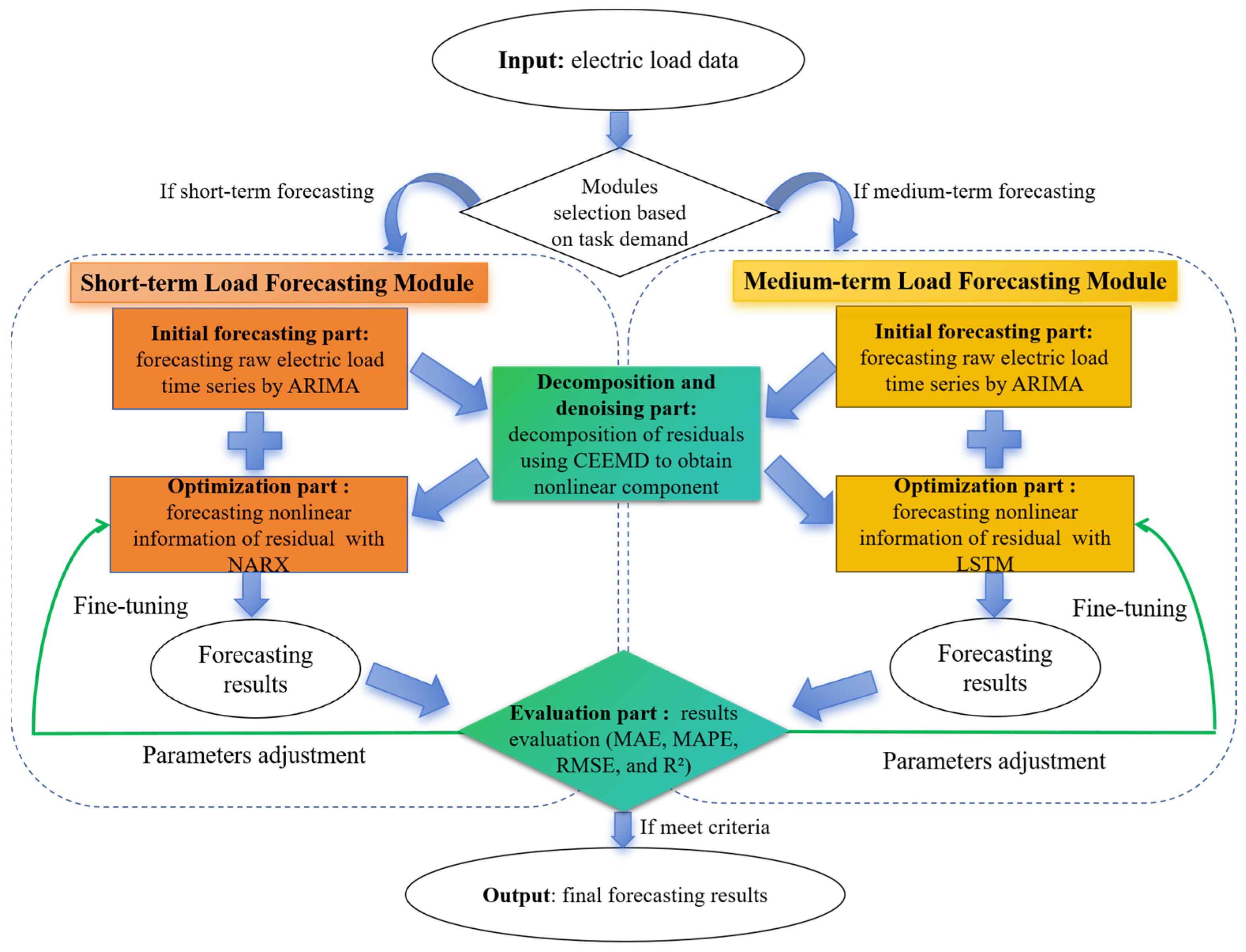
A CMPLF method that fuses hierarchical optimization models is proposed in this study to address the challenge of fitting the nonlinear residuals, aiming to improve the accuracy of short- and medium-term power load forecasting. The method divides the power load-forecasting problem into short-term and medium-term forecasting based on the dataset’s time unit length. Specifically, for short-term power load prediction [35,36], we chose the ARIMA model to finish preliminary load forecasting and mined its internal linear information. After deriving the forecast residuals, we used the CEEMD algorithm to decompose the nonlinear components in the residuals. The NARX model then was used to analyze the short-term dependence between the load residuals and power load to make a comprehensive prediction. For medium-term load prediction [37,38], considering the extensive data period, the ARIMA model, utilized for forecasting the linear aspects of the data, remained unchanged. The LSTM model was employed to fit the nonlinear elements within the residuals of the ARIMA model, analyzing the long-term dependencies among the load residuals. The final forecasting results were derived by integrating predictions from both linear and nonlinear models. This fusion approach also incurs certain costs. Model integration increases system complexity, requiring more computational resources and time for training and validation. However, our method significantly improves the accuracy of power load forecasting. The primary contributions of this work can be condensed into three aspects:

• A hierarchical optimization method is developed for accurate power load prediction, including the initial forecasting model, decomposition and denoising strategy, and efficient nonlinear optimization algorithms based on two forecasting modules.
• In this highly precise forecasting method, by breaking through bottlenecks in hierarchical model fusion, three emerging models, i.e., an ARIMA model, a NARX model, and LSTM networks are effectively fused.
• The superiority and validity of the CMPLF method are confirmed through two forecasting experiments using 30 min interval power load data from Queensland provided by the Australian Energy Market Operator (AEMO). This work proves that the proposed CMPLF method is suitable for the samples of different regions.

The rest of this paper is structured as follows: Section 2 presents the overview and flowchart of our proposed CMPLF method via deep learning. The short-term load-forecasting and medium-term load-forecasting modules in the CMPLF method are then described. Subsequently, every part and the algorithms in the two modules are introduced in detail. In Section 3, we used the dataset from the 10th Teddy Cup Data Mining Challenge in 2022 to train the models to improve the accuracy of power load forecasting. To verify the superiority and validity of the CMPLF method, we accomplished three experiments via different datasets in Section 4. Eventually, Section 5 provides a summary of the entire paper, drawing conclusions and proposing future work directions.

2. The Proposed CMPLF Method

This section provides an overview of the proposed CMPLF method, which aims to solve the problem of fitting the nonlinear part of the residuals and improve the accuracy and stability of power system load forecasting. The structure and flowchart of the CMPLF method are first given. Subsequently, the two modules of the CMPLF method are introduced in detail, respectively. Eventually, the specific content of each part is designed while a summary of the deep learning models and elevation metrics are presented.

2.1. Overview of the Proposed CMPLF Method

A structural overview of the proposed CMPLF method is shown in Figure 1, illustrating the flowchart of the load prediction method. Firstly, based on the input load data, we categorize power load forecasting into short-term forecasting and medium-term forecasting. Each module has four parts, namely the initial forecasting part, decomposition and denoising part, optimization part, and evaluation part, which are tightly related and reflect the integrity of power load forecasting. After receiving the forecasting results obtained from the combination prediction of linear and nonlinear models, we put them into the evaluation part to judge if they meet the criteria. If the results do not meet the criteria, the parameters of the models will be fine-tuned. Instead, the forecasting results are output.

2.2. Design of the CMPLF Method

2.2.1. Design Philosophy of the CMPLF Method

As we all know, the power system load has complex characteristics in practice. Its trend cannot be described simply as linear or nonlinear but exists objectively in the form of Figure 2.

Due to the complex forms of the existence of the power system load, a single prediction model cannot make a comprehensive extraction and training of its features. Therefore, a medium is needed to integrate predictive models from different domains to enable the prediction of the complex forms of load data. CEEMD is commonly used in signal processing, fault diagnosis, and data analysis. Its rationality in data decomposition is that it can effectively separate the endowment modal functions at different scales. So, CEEMD can be used as an efficient integration medium when analyzing the power system load, a target with complex compositions.

2.2.2. Short-Term Load-Forecasting Module

The short-term load-forecasting module consists of four parts: the ARIMA model, CEEMD algorithm, NARX model, and evaluation part. To accurately achieve short-term power load forecasting, the ARIMA model is utilized to mine the linear information of the electrical load. After deriving the prediction residuals, we use the CEEMD algorithm to decompose the nonlinear components in the residuals. Then, the NARX model is employed to analyze the short-term dependence among the load residuals to obtain the integrated prediction results. In the last step, we use four evaluation indexes to evaluate and revise the models. The flowchart of the short-term load-forecasting module is presented below in Figure 3.

Here, X₁ to X₅ is the nonlinear component of power load residuals, ω is the hidden layer weights, Sigm is the activation function, and P₁ to P₅ is the predicted value of the nonlinear component of the residuals. So, we can know how the short-term load-forecasting module works from Figure 3.

2.2.3. Medium-Term Load-Forecasting Module

The medium-term load-forecasting module consists of four parts: the ARIMA model, CEEMD algorithm, LSTM model, and evaluation part. To accurately achieve medium-term power load forecasting, we still use the ARIMA model to mine the linear information. The CEEMD algorithm is then adopted to decompose the nonlinear components in the residuals. The LSTM model is used for medium-term prediction and then we analyze the long-term dependence among the load residuals. Eventually, the two forecasting results are combined to produce the final medium-term load-forecasting results. We also use four evaluation indexes to evaluate and revise the models. The flowchart of the medium-term load-forecasting module is shown as follows in Figure 4.

Same as the short-term load-forecasting module, where X₁ to X₅ is the nonlinear component of power load residuals, σ is the hidden layer weights, tanh is the activation function, and P₁ to P₅ is the predicted value of the nonlinear component of the residuals. Therefore, we can know how the medium-term load-forecasting module works from Figure 4.

2.3. Theoretical Basis

2.3.1. Initial Forecasting Part

ARIMA Model

The autoregressive difference moving average model, or ARIMA [39] model, is a model proposed by Box and Jenkins. ARIMA separates signal and noise by using past observations while considering differential, autoregressive, and moving average components. ARIMA requires its data to be smooth, and it needs to convert the unstable data into smooth data by multiple differences or finding co-integration relationships when dealing with unstable data. Its composition consists of an autoregressive (AR) process and a moving average (MA) process. It is difficult for the traditional regression model to fit the dataset effectively and reasonably when the predicted dataset has a significant cyclical trend in time with too many factors affecting its development and change. At this point, ARIMA shows its unique advantages as a typical time series analysis model. The original time series model is shown in Equation (1):

$$(1-{\displaystyle \sum _{i=1}^p{\alpha }_i}{L}^i){(1-L)}^d{y}_t={\alpha }_0+(1+{\displaystyle \sum _{i=1}^q{\beta }_i}{L}^i){\epsilon }_t$$

(1)

where L is the lag operator of y, which satisfies: $L^i{y}_t=y_{t-i}$; y_t is the output power prediction; and y_t−i is the power value for the previous time step. β is the regression coefficient, α_i is the coefficient determined by difference equations, and ε_t is the perturbation term.

The module is used to perform the first prediction on the preprocessed dataset, mainly dealing with the linear features in the dataset. By capturing the trend and seasonal components of the time series, the ARIMA model can provide a preliminary forecasting result. This module performs well in dealing with long-term trends and cyclical fluctuations in electric load data but is limited in its ability to handle nonlinear features.

2.3.2. Decomposition and Denoising Part

CEEMD Algorithm

CEEMD [40] is a multi-scale signal decomposition technique for decomposing nonlinear and non-stationary signals. It is a decomposition method that obtains several IMFs and a residual term through a series of iterations of the signal. CEEMD aims to solve the “residual auxiliary noise” problem of EEMD. CEEMD overcomes the problem of mode confusion and convergence difficulty of the traditional Empirical Mode Decomposition (EMD) by adaptively correcting noise and locking local characteristic frequency for each local oscillation mode. It can extract the local characteristics of signals more accurately with better robustness and stability. Therefore, CEEMD is widely used in signal analysis, pattern recognition, and time series forecasting, such as power system load forecasting. It can be used to decompose the nonlinear components to further improve prediction accuracy.

The module is used to extract the nonlinear components from the processed residuals of the ARIMA model. By decomposing the residuals, the CEEMD algorithm can decompose complex nonlinear signals into several IMFs. These IMFs represent the different frequency components of the data. The process provides the basis for subsequent time series network models to deal with nonlinear features.

2.3.3. Optimization Part

NARX Model

The NARX [41,42] is a model for short-term time series forecasting. This model can handle nonlinear, dynamic, complex, and noisy time series data. Specifically, NARX consists of two parts: the autoregressive part and the external variable part. The autoregressive part is a feedforward neural network, which takes its historical input at the current time as input and predicts the output value at the current time. The external variable part takes external variable input as auxiliary input of the model, these external variables can be other data related to the current time or information from the external environment. NARX needs to be trained to determine the weights and bias parameters of the model, which usually uses the error backpropagation algorithm for training. In the prediction process, the known historical data and external variables are input into the model, and the prediction results in the future time can be generated by the model.

The module is used for short-term nonlinear time series forecasting, which can handle dynamic, complex, and noisy data. By processing the nonlinear features of the data decomposed by the CEEMD algorithm, the NARX model can provide further prediction results for the nonlinear sequences of electric load.

LSTM Model

LSTM [4,30] is a commonly used modified model of the recurrent neural network (RNN) [43]. It introduces a gating mechanism based on RNN, which allows the LSTM model to decide when to update the information stored in each neuron. The main component structures of LSTM are the input gate $i_t$, forgetting gate $f_t$, and output gate $o_t$. Moreover, in the gate structure, $c_t$ denotes the current state of the cell, $h_t$ denotes the hidden layer state, and $x_t$ is the input data. Firstly, in the input layer, the original fault time series is defined as $F_0=\left\{f_1,f_2,\cdots ,f_n\right\}$. Then, the divided training set and test set can be expressed as $F_{\mathrm{tr}}=\left\{f_1,f_2,\cdots ,f_m\right\}$ and $F_{\mathrm{te}}=\left\{f_{m+1},f_{m+2},\cdots ,f_n\right\}$. The constraints $m<n$, $m,n\in N$ are satisfied, then the elements $f_t$ in the training set are normalized, and the normalized training set is ${F\prime }_{\mathrm{tr}}=\left\{{f\prime }_1,{f\prime }_2,\cdots ,{f\prime }_m\right\}$.

To adapt to the characteristics of the hidden layer input, the data segmentation method is applied to the process $F_{tr}^{\prime }$. The segmentation window length is set to L. The input of the segmented model is $\mathrm{X}=\left\{X_1,X_2,\cdots ,X_L\right\}$, and the corresponding theoretical output is $Y=\left\{Y_1,Y_2,\cdots ,Y_L\right\}$. Input X into the hidden layer, which contains L isomorphic LSTM cells connected by anterior–posterior moments. Set the cell state vector size to $S_{state}$, then both $C_{P-1}$ and $H_{P-1}$ vectors are of a size $S_{state}$. Apply the trained $LSTM$ network (denoted as $LST{M}_{net}^{*}$) for prediction. The prediction process uses an iterative approach, first theoretically outputting the last row of data for Y as $F_f=\left\{{f\prime }_{m-L+1},{f\prime }_{m-L+2},\cdots ,{f\prime }_m\right\}$, inputting $F_f$ into $LST{M}_{net}^{*}$ to output the results, and then combining the last L − 1 data points of $Y_f$ and $P_{m+1}$ into a new row of data shown as Equation (2):

$$Y_{f+1}=\left\{{f\prime }_{m-L+2},{f\prime }_{m-L+3},\cdots ,{f\prime }_{m+1}\right\}$$

(2)

Input $Y_{f+1}$ into $LST{M}_{net}^{*}$, then the prediction value at m + 2 is $P_{m+2}$. By analogy, the prediction sequence obtained is $P_0=\left\{P_{m+1},P_{m+2},\cdots ,P_n\right\}$. Next, the $P_0$ inverse normalization of $z-score$ (denoted as $de\_zscore$) is performed to obtain the final prediction sequence corresponding to the test set $F_{te}$ as $Pte=de\_zscore(P0)=\left\{P_{m+1}^{\ast },P_{m+2},\cdots P_n^{\ast }\right\}$, where

$$p_k^{\ast }=p_k\sqrt{{\displaystyle \sum _{t=1}^n{\left(ft-{\displaystyle \sum _{t=1}^{n}ft/n}\right)}^2/n}}+{\displaystyle \sum _{t=1}^{n}ft/n}m+1\le k\le n,k\in N$$

(3)

The module is used for long-term nonlinear time series forecasting. Time series networks can capture dependencies in time series through their special lagging mechanism and thus, model nonlinear features. By training the LSTM model, we are able to accurately predict the extracted nonlinear components, reducing the error and improving the overall model performance.

2.3.4. Evaluation Part

To assess the accuracy of the models, we apply four model evaluation indices in the forecasting result evaluation section: MAE, MAPE, RMSE, and R².

MAE is the expected value of absolute error predicted by the model. The lower the value of MAE, the better the precision of the model for describing the overall experimental data. The formula is shown in Equation (4):

$$MAE={\displaystyle \frac{1}{N}}{\displaystyle \sum _{i=1}^n|y_i}-{\widehat{y}}_i|$$

(4)

where N represents the sample size, $y_i$ denotes the actual sample value, and ${\widehat{y}}_i$ signifies the predicted value of the model.

MAPE refers to the average of the absolute value of the deviation between each observed value and the arithmetic mean value. The result is expressed as a percentage to make it more intuitive. A smaller MAPE indicates a smaller expectation of the variance between the predicted value and the actual value, showing higher accuracy for the model. The formula is as follows:

$$MAPE={\displaystyle \frac{1}{N}}{\displaystyle \sum _{i=1}^n\left|\frac{{\widehat{y}}_i-y_i}{y_i}\right|}\times 100\%$$

(5)

RMSE can be defined as the square root of the quotient of the square of the difference between the predicted value and the true value divided by the number of observations n. The smaller the RMSE value, the more accurate the model is in predicting the data. The formula is as follows:

$$RMSE=\sqrt{{\displaystyle \frac{{\displaystyle \sum _{i=1}^n{(y_i-{\stackrel{⌢}{y}}_i)}^2}}{N}}}$$

(6)

R² is a statistical measure of the goodness-of-fit of a regression model that expresses the overall relationship between the dependent variable and all the independent variables. R² is equal to the ratio of the regression sum-of-squares to the total sum-of-squares, i.e., the percentage of the variability in the dependent variable that is explained by the regression equation (in MATLAB (R2023b), R² = 1—the ratio of the regression sum-of-squares to the total sum-of-squares). Of the error between the actual and mean values, the regression error and the residual error are in a reciprocal relationship. Thus, the regression error determines the R² of the linear model from the positive side, and the residual error determines the R² of the linear model from the negative side. The maximum value of R² is 1. The closer the value of R² is to 1, the better the regression line fits the observations. In contrast, the smaller the value of R² is, the poorer the fit of the regression line to the observations. The formula is as follows:

$$R^2=1-{\displaystyle \frac{\sum {\left(y-\widehat{y}\right)}^2}{\sum {\left(y-\overline{y}\right)}^2}}$$

(7)

3. Experimental Analysis

In this section, the data coming from the 10th Teddy Cup Data Mining Challenge in 2022 was used to train the models. These data were provided in a mathematics modeling competition, which was available at http://www.tipdm.com/ (accessed on 23 July 2023). For short-term load forecasting, the regional 15 min load data were used to predict the power load of the region in the future and analyze the prediction accuracy. For medium-term load forecasting, the daily load values would be predicted according to the load dataset provided from a region in mainland China.

3.1. Training of Short-Term Load-Forecasting Model

3.1.1. Dataset Analysis

To study the variation in the power load with time from 1 January 2018, to 31 August 2021, the NARX model and ARIMA model were combined in this paper. Moreover, the CEEMD algorithmic decomposition was performed before fitting the NARX model. First, the ARIMA model was used to fit the raw power load series while the NARX model was used to fit the nonlinear information in the residual of the ARIMA model mined by the CEEMD algorithm. In this way, the linear part and nonlinear part of the power load time series were fitted, respectively. The accuracy of short-term load forecasting was improved.

3.1.2. Establishment of ARIMA Model

After importing the 15 min daily load data from 2018 to 2021 into SPSS25 (V25.0.0), the corresponding time variables were defined and plotted as a time series diagram. The analysis shows that the total active power fluctuates around a certain value with time. Due to the total active power fluctuating greatly with time, we judge that the time series is non-stationary and needs to be treated with a difference. To reduce the data loss caused by the difference as much as possible, the first-order difference is used to determine the ARIMA (p, d, q) parameters d for 1.

Due to p, d in the ARIMA model was determined by the autocorrelation coefficient (ACF) and the partial autocorrelation coefficient (PACF), respectively. We made the ACF and PACF plots of the series after the first-order difference. It can be seen that the lag number of the ACF is truncated after 2, and the lag number of the PACF is truncated after 1. Both ACF and PACF of the data have trailing phenomena while the ACF is out of the confidence interval at lag number 2 seen from the graphs. Therefore, we judge that p is taken as 2 in the ARIMA model. The PACF is outside the confidence interval when the lag number is 8, so we judge that the value of q in the model is 8.

The parameters of the ARIMA model given by SPSS are shown in

Table 1. The parameters of the ARIMA model.

			Estimate	Standard Error	t	Significance
ARIMA (2,1,8)	Constant		2.112	134.024	0.016	0.987
	AR	Delay 1	−0.744	0.025	−29.717	0.000
		Delay 2	0.251	0.025	10.053	0.000
	Difference		1.000
	MA	Delay 1	−0.360	0.024	−15.290	0.000
		Delay 2	0.711	0.016	44.589	0.000
		Delay 3	−0.202	0.014	−13.933	0.000
		Delay 4	−0.568	0.011	−53.706	0.000
		Delay 5	0.093	0.014	6.461	0.000
		Delay 6	0.464	0.010	46.091	0.000
		Delay 7	−0.157	0.011	−14.760	0.000
		Delay 8	−0.349	0.008	−41.923	0.000
Time	Molecule	Delay 0	−0.001	0.018	−0.044	0.965

:

In the ARIMA (2,1,8) model shown in Table 1, ${\alpha }_0$ = 2.112, ${\alpha }_1$ = −0.744, ${\alpha }_2$ = 0.251, and ${\epsilon }_t$ = −0.001. The expressions of the ARIMA (2,1,8) model were derived by substituting ${\alpha }_0$, $\beta$, and ${\epsilon }_t$, then simplifying as Equation (8):

$$y_t={\displaystyle \frac{2.112-(1+{\sum }_{i=1}^8{\beta }_i{L}^i)\times 0.001}{(1+0.744L-0.251L^2)(1-L)}}$$

(8)

The ARIMA model fitting results obtained by SPSS are shown in

Table 2. ARIMA model statistics.

Model	Fit Statistics	Young-Box Q (18)			Number of Outliers
	Stationary R-Square	Statistics	DF	Significance
ARIMA (2,1,8)	0.760	3901.733	8	0.103	0

:

Table 2 shows that the R² of the model is 0.760. The significance test yields a p-value of 0.103. This indicates that the original hypothesis is accepted at a 95% confidence level, i.e., the white noise series is considered to be the residuals. Since the ARIMA model has some errors in the total active power prediction, the prediction analysis should be performed after the nonlinear mining of its residuals.

3.1.3. Mining Nonlinear Information of Residual via CEEMD

While the ARIMA model has demonstrated good performance in fitting power system load, its fundamental linearity makes it susceptible to distortion when handling nonlinear data. Therefore, the CEEMD algorithm was used to deal with the residual produced by the ARIMA model to decompose its nonlinear components in the experiments.

The original residual dataset was decomposed by adding conjugate white noise, and the results of each decomposition were visualized to detect the outlier data. Then, the box plot was drawn as shown in Figure 5. When the number of decompositions reached 7, the outlier data completely disappeared. The decomposed data showed set monotonicity, i.e., the nonlinear components in the residuals were all removed.

Figure 6 below shows, after nine decompositions by the CEEMD algorithm, the results of the prediction residuals of the ARIMA model. The results show that the data are significantly linear after seven decompositions. The results of the first seven decompositions are superimposed and processed to constitute the nonlinear components of the residuals for further analysis. This work can complement the forecasting results of the ARIMA model.

3.1.4. Residual Prediction Analysis via NARX

To study the load of the power system in the region at fifteen-minute intervals, the NARX model was developed to mine the nonlinear components of the residuals.

Parameter Determination

The hidden layer is tasked with processing the features of the input data samples. The delay is the rectification of the state of the update unit of the time series network. As the number of network layers increases, the accuracy of the model rises, but at the same time, the complexity of the model increases. Moreover, the computational consumption and risk of overfitting also increase significantly. The higher the delay time, the higher the accuracy of the model to establish long-term dependence between data samples, but at the same time, it will also face the problems of computational cost and overfitting risk. Considering the game between the number of samples and the prediction accuracy of the model, a 30-layer network with five delays was selected to build the model.

Choice of Activation Function

The essence of the learning ability of neural networks is to optimize their parameters through training the feedback of error. Therefore, the error of the current layer is closely related to the choice of the activation function. Due to the large amount of data in the training set in the short-term load forecasting, if the ReLU function or tanh function is chosen as the activation function, neither of its derivative values may be greater than one, which makes the gradient disappear during the iteration process and leads to the early termination of training. Therefore, we chose to use the sigmoid function as the activation function. Moreover, the neurons with the derivative value of one chosen for learning could effectively avoid the gradient disappearance phenomenon and make the model training complete smoothly.

After the model parameters and activation functions were determined, the NARX model was established. The nonlinear residuals extracted by CEEMD were imported into the built NARX model and the training was started. The proportion of the training set, generalization set, and test set is 14:3:3. In the last step, the residual predictions from NARX were replenished to the ARIMA model results to acquire the final forecasting results. See Figure 7.

From Figure 7, it can be seen that the ARIMA-NARX model fits the actual values greatly, and its prediction results are very accurate. It is indicated that our proposed ARIMA-NARX model and its forecasting effect have wonderful significance on short-term load forecasting, which is also instructive for actual production. Additionally, the R² of the ARIMA-NARX mentioned in Section 4 is 0.983 on this dataset can prove it well.

3.2. Training of Medium-Term Load-Forecasting Model

3.2.1. Dataset Analysis

To study the variation in the daily power load values over time for each day from 1 January 2018, to 31 August 2021, for the power grid in this region, we combined the LSTM model with the ARIMA model and performed the CEEMD decomposition process before fitting the LSTM model. First, the ARIMA model was used to fit the daily power load sequences. Then, we chose the LSTM model to fit the residuals of the ARIMA model to exploit the nonlinear information in them. In this way, the linear and nonlinear parts of the power load time series were fitted separately to enhance the accuracy of medium-term power load forecasting.

3.2.2. Linear Information Fitting and Nonlinear Information Extraction

To analyze the daily power load values in the region over time, this research first utilized the ARIMA model to fit the daily values of the power load in the region. The ARIMA (1,1,14) model of the daily power load values was established. The expression is as follows:

$$y_t={\displaystyle \frac{85.639-(1+{\displaystyle \sum _{i=1}^{14}{\beta }_i{L}^i})\times 0.214}{(1+0.569L)(1-L)}}$$

(9)

The prediction results were compared with the real values to derive the prediction residuals. The nonlinear information was extracted using the CEEMD algorithm, in which the time series was decomposed into nine IMF components and one residual term. Then, the decomposition results were obtained by summing the first seven nonlinear terms. The results were substituted into the LSTM model to fit the residuals.

3.2.3. Nonlinear Information Prediction via LSTM

In this research, LSTM was used to predict the nonlinear residuals of the ARIMA model extracted from CEEMD. The training and testing sets were set to 70% and 30%, respectively, while the initial learning rate of the LSTM model was set to 0.1. The learning rate was multiplied by a factor of 0.5 after 300 iterations to prevent the overfitting of the model. The time dimension parameter was set to 30, while the numbers of implied units and iterations were set to 250 and 500. The data obtained from CEEMD was imported into MATLAB and then computed. The prediction results of the training set and its fitting error are shown in Figure 8:

The model training result shows that the RMSE of the LSTM model converges to 0.13 after about 400 iterations. The comparison between the predicted values with the true values reveals that the LSTM has a great prediction effect for the testing set. Therefore, it is found that the LSTM model achieves better results in predicting the nonlinear residuals of the ARIMA model.

Lastly, the predictions of the LSTM model were added with the forecasting results of the ARIMA model to obtain the final prediction results. The final forecasting results of the daily power load are shown in Figure 9.

From Figure 9, it is clear that the ARIMA-LSTM model is a terrific fit for the actual values and its prediction results are greatly accurate. It proves that our proposed ARIMA-LSTM model and its forecasting effect have important significance on medium-term load forecasting, which is also instructive for actual production. Additionally, the R² of the ARIMA-LSTM mentioned in Section 4 being 0.987 on this dataset can prove it well.

4. Performance Evaluation

In this section, three experiments are introduced objectively to validate the performance and superiority of the proposed CMPLF method. Before that, the dataset involved in the experiments must be set up.

4.1. Dataset Setting

The experiments in this paper used 30 min interval power load data from Queensland, Australia in 2023, which is available at https://aemo.com.au/ accessed on 11 August 2023. The 30 min interval power load data of Queensland is from 8 June 2023, to 12 July 2023. We divided the operational load data into 5 groups according to weeks, of which 70% was chosen as the training set and the remaining 30% was automatically included in the testing set.

4.2. Experiment I: Performance of the CMPLF Method Compared with Basic Models

4.2.1. Comparison of Short-Term Load-Forecasting Models

To test the effect of the ARIMA-NARX model on short-term forecasting, the MAPE, RMSE, and R² of the ARIMA model, NARX model, and ARIMA-NARX model were calculated on the dataset, respectively. The results are shown in

Table 3. Comparison of the precision of the different models (short-term).

Model	Evaluation Indicators
	MAPE	RMSE	R-Square
ARIMA	0.0579	0.417	0.897
NARX	0.0324	0.245	0.919
Our model	0.0231	0.146	0.983

:

Table 3 shows that the ARIMA-NARX model fits with less error than the conventional ARIMA model and NARX model, i.e., it has a better prediction effect. Compared with the original ARIMA model, the MAPE and RMSE of the ARIMA-NARX model for the test set predictions are reduced by 60.1% and 64.9%, respectively. The R² of the ARIMA-NARX model is enhanced by 9.6% over the ARIMA model. Compared with the original NARX model, the MAPE and RMSE of the ARIMA-NARX model for the test set predictions are reduced by 28.7% and 40.4%, respectively. Moreover, the R² of the ARIMA-NARX model is improved by 7.0% over the NARX model. It is clear that ARIMA-NARX has a significant performance improvement over the basic models in short-term power load forecasting.

4.2.2. Comparison of Medium-Term Load-Forecasting Models

To test the performance of the ARIMA-LSTM model on medium-term forecasting, the MAPE, RMSE, and R² of the ARIMA model, LSTM model, and ARIMA-LSTM model were calculated on the dataset, respectively. The results are shown in

Table 4. Comparison of the precision of the different models (medium-term).

Model	Evaluation Indicators
	MAPE	RMSE	R-Square
ARIMA	0.0579	0.417	0.897
LSTM	0.0318	0.229	0.924
Our model	0.0223	0.138	0.987

:

From the analysis of the data in Table 4, it is evident that the ARIMA-LSTM model fits with less error than the traditional ARIMA model and LSTM model, i.e., it has better prediction results. Compared with the original ARIMA model, the MAPE and RMSE of the ARIMA-LSTM model for the test set predictions are reduced by 61.5% and 66.9%, respectively. The R² of the ARIMA-LSTM model is enhanced by 10.0% over the ARIMA model. Compared with the original LSTM model, the ARIMA-LSTM model reduces its MAPE and RMSE by 29.9% and 39.7%, respectively. Moreover, the R² of the ARIMA-LSTM model is improved by 6.8% over the LSTM model. It can be concluded that ARIMA-LSTM has a significant performance improvement over the original models in medium-term power load forecasting.

The experimental data in Part 4.2 shows the proposed ARIMA-NARX model and the ARIMA-LSTM model provide good performance in forecasting the daily power load of a region in mainland China with much better accuracy than the simple, existing deep learning models. Therefore, we combine the two hybrid models to integrate the CMPLF method. The method is a recommended deep learning method for forecasting the short- and medium-term power load of a region.

4.3. Experiment II: Validity of the CMPLF Method on Cross-Regional Datasets

To verify the validity of our proposed CMPLF method, we used the dataset from Queensland to examine the accuracy of the models. MATLAB was used to finish this experiment to show the validity of this forecasting method on cross-regional datasets.

Figure 10 shows the fitness of short-term load forecasting. The horizontal coordinate of this graph is the true load, while the vertical coordinate is the load predicted by the ARIMA-NARX model. The line band Y = x refers to the case where the predicted and actual loads are equal. The distance of each point (blue) plotted with the data predicted by our model from this center line represents the magnitude of the error. The lower the dispersion of all the scattered points, the greater the model. Conversely, the lower the accuracy of the model. It shows that the prediction results have a low degree of discretization from this center line. Therefore, we can obtain that the ARIMA-NARX algorithm has an accurate prediction effect on short-term power load forecasting.

Figure 11 shows the fitness of medium-term load forecasting. The horizontal coordinate of this graph is the true load while the vertical coordinate is the load predicted by the ARIMA-LSTM model. The line band Y = x refers to the case where the predicted and actual loads are equal. The distance of each point (red) plotted with the data predicted by our model from this center line represents the magnitude of the error. The lower the dispersion of all the scattered points, the greater the model. Conversely, the lower the accuracy of the model. It shows that the prediction results have a low degree of discretization from this center line. Therefore, we can obtain that the ARIMA-LSTM algorithm has an accurate prediction effect on medium-term power load forecasting.

Therefore, Experiment II can verify the CMPLF method applies to cross-regional datasets.

4.4. Experiment III: Superiority of the CMPLF Method Compared with the SOTA Prediction Methods

To show the superiority of our models in the CMPLF method on power load forecasting and to compare with some existing mainstream models, the experiment took two deep learning methods: the PSO-LSTM model and the GWO-BP model into comparison. Our simulation referred to the actual data collected from June 2023 to July 2023 by AEMO.

Figure 12 exhibits the comparison between the forecasting results and real data on short-term load forecasting using the ARIMA-NARX model, PSO-LSTM model, and GWO-BP model.

Based on the prediction results, this experiment also calculated the MAE, MAPE, and R² for the different models. These two conventional error criteria can show the specific effect of each forecasting model. The detailed results are displayed in

Table 5. Comparison of the error criteria of the three forecasting models (short-term).

Model.	Evaluation Indicators
	MAE	MAPE	R-Square
PSO-LSTM	63.5548	0.0559	0.8881
GWO-BP	67.1038	0.0595	0.8762
Our method	54.1754	0.0488	0.9104

.

From the above table, we can clearly know that the proposed ARIMA + NARX combining method performs the best result in short-term power load forecasting compared with the other methods.

Figure 13, on the other hand, shows the comparison between the prediction results and real data on medium-term load forecasting using the ARIMA-LSTM model, PSO-LSTM model, and GWO-BP model.

Based on the forecasted data, this experiment also calculated the MAE, MAPE, and R² for the different models. These two conventional error criteria can show the specific effect of each forecasting model. The detailed results are shown in

Table 6. Comparison of the error criteria of the three forecasting models (medium-term).

Model	Evaluation Indicators
	MAE	MAPE	R-Square
PSO-LSTM	63.3017	0.0548	0.9131
GWO-BP	76.7714	0.0661	0.8621
Our method	54.3116	0.0472	0.9222

.

From the above table, we can clearly know that the proposed ARIMA + LSTM combining method performs the best result in medium-term power load forecasting compared with the other methods.

Furthermore, to better represent the superiority of our proposed ARIMA-NARX model and the ARIMA-LSTM model on short- and medium-term load forecasting, we made two relative error box-scatter plots based on the forecasted data. See Figure 14.

From Figure 14, these unevenly distributed points can also clearly verify that the combined models in our proposed CMPLF method have a superior forecasting effect on short- and medium-term load forecasting compared with some existing mainstream models.

Although the CMPLF method uses a combination of the ARIMA model and time series networks and outperforms a single model in terms of evaluation metrics, it still suffers from some errors. These errors may arise from the fact that the ARIMA model assumes that the time series are linear and that the statistical properties do not vary over time. In addition, the time series networks may be deficient in handling long time dependencies and incomplete data noise rejection. Also, the ARIMA model and the time series networks have inadequate hyperparameter optimization, as well as the complexity of the power system and external factors can generate errors.

Considering the development of the models, the errors can be further reduced by introducing more advanced models and automated parameter optimization techniques using data cleaning and feature engineering to remove noise, and incorporating external factors to increase the sensitivity of the models to external changes.

5. Conclusions and Future Work

Our study proposes a CMPLF method based on the fusion of hierarchical optimization models, namely ARIMA-NARX and ARIMA-LSTM, which is utilized to forecast short- and medium-term load. In this work, a combination to fuse the ARIMA model with the NARX model and the LSTM model is worked to the problem of fitting the nonlinear part of the residuals. The CMPLF method has two modules to forecast short-term load and medium-term load, respectively. Experiment I reveals that the fitting performance of both ARIMA-NARX and ARIMA-LSTM is better than that of ARIMA, NARX, and LSTM on the dataset from a region of mainland China. Included among these, the R² of the ARIMA-NARX and ARIMA-LSTM models are 0.983 and 0.987 on this dataset, respectively. Therefore, this forecasting method, based on the hybrid algorithm of ARIMA-NARX and ARIMA-LSTM, can predict the short-term and medium-term power load more accurately. In Experiment II, the goodness-of-fit values are 97.174% for the ARIMA-NARX model and 97.162% for the ARIMA-LSTM model based on the data of the Queensland power grid. The results of this experiment using the power grid dataset from Queensland fully demonstrate the validity of the CMPLF method proposed in this paper. Furthermore, to more clearly verify the superiority of our proposed CMPLF method, Experiment III takes some existing mainstream forecasting methods into comparison. The data illustrates that the CMPLF method has the best performance. Our work will be instructive for achieving sustainability in energy management systems.

Although the proposed CMPLF method shows good results on the provided power load dataset, the models are based on the basic assumption that the future power load is only influenced by its historical value. This simplifies the real situation. In practice, there are many factors affecting the region’s electric load. For example, government policies and the socioeconomic environment also have a significant impact on the industry’s electric consumption. Therefore, it is the future research direction to combine more reasonable factors influencing power load and establish more accurate power load-forecasting models.

References

1. Xie, L.; Wu, J.; Li, Y.; Sun, Q.; Xi, L. Automatic generation control strategy for integrated energy system based on ubiquitous power internet of things. IEEE Internet Things J. 2022, 10, 7645–7654. [Google Scholar] [CrossRef]
2. Wang, J.; Gao, J.; Wei, D. Electric load prediction based on a novel combined interval forecasting system. Appl. Energy 2022, 322, 119420. [Google Scholar] [CrossRef]
3. Solyali, D. A Comparative Analysis of Machine Learning Approaches for Short-/Long-Term Electricity Load Forecasting in Cyprus. Sustainability 2020, 12, 3612. [Google Scholar] [CrossRef]
4. Pavlatos, C.; Makris, E.; Fotis, G.; Vita, V.; Mladenov, V. Enhancing Electrical Load Prediction Using a Bidirectional LSTM Neural Network. Electronics 2023, 12, 4652. [Google Scholar] [CrossRef]
5. Soyler, I.; Izgi, E. Electricity Demand Forecasting of Hospital Buildings in Istanbul. Sustainability 2022, 14, 8187. [Google Scholar] [CrossRef]
6. Tang, J.; Saga, R.; Cai, H.; Ma, Z.; Yu, S. Advanced Integration of Forecasting Models for Sustainable Load Prediction in Large-Scale Power Systems. Sustainability 2024, 16, 1710. [Google Scholar] [CrossRef]
7. Wang, X.; Yao, Z.; Papaefthymiou, M. A real-time electrical load forecasting and unsupervised anomaly detection framework. Appl. Energy 2023, 330, 120279. [Google Scholar] [CrossRef]
8. Laitsos, V.; Vontzos, G.; Bargiotas, D.; Daskalopulu, A.; Tsoukalas, L.H. Enhanced Automated Deep Learning Application for Short-Term Load Forecasting. Mathematics 2023, 11, 2912. [Google Scholar] [CrossRef]
9. Jayashankara, M.; Shah, P.; Sharma, A.; Chanak, P.; Singh, S.K. A novel approach for short-term energy forecasting in smart buildings. IEEE Sens. J. 2023, 23, 5307–5314. [Google Scholar] [CrossRef]
10. Korkas, C.; Dimara, A.; Michailidis, I.; Krinidis, S.; Marin-Perez, R.; Martínez García, A.I.; Tzovaras, D. Integration and Verification of PLUG-N-HARVEST ICT Platform for Intelligent Management of Buildings. Energies 2022, 15, 2610. [Google Scholar] [CrossRef]
11. Khan, S.U.; Khan, N.; Ullah, F.U.M.; Kim, M.J.; Lee, M.Y.; Baik, S.W. Towards intelligent building energy management: AI-based framework for power consumption and generation forecasting. Energy Build. 2023, 279, 112705. [Google Scholar] [CrossRef]
12. Wu, D.; Lin, W. Efficient residential electric load forecasting via transfer learning and graph neural networks. IEEE Trans. Smart Grid 2022, 14, 2423–2431. [Google Scholar] [CrossRef]
13. Lv, L.; Wu, Z.; Zhang, J.; Zhang, L.; Tan, Z.; Tian, Z. A VMD and LSTM based hybrid model of load forecasting for power grid security. IEEE Trans. Ind. Inform. 2022, 18, 6474–6482. [Google Scholar] [CrossRef]
14. Lin, X.; Zamora, R.; Baguley, C.A.; Srivastava, A.K. A hybrid short-term load forecasting approach for individual residential customer. IEEE Trans. Power Deliv. 2022, 38, 26–37. [Google Scholar] [CrossRef]
15. Chan, K.Y.; Yiu, K.F.C.; Kim, D.; Abu-Siada, A. Fuzzy Clustering-Based Deep Learning for Short-Term Load Forecasting in Power Grid Systems Using Time-Varying and Time-Invariant Features. Sensors 2024, 24, 1391. [Google Scholar] [CrossRef] [PubMed]
16. Tudose, A.M.; Sidea, D.O.; Picioroaga, I.I.; Boicea, V.A.; Bulac, C. A cnn based model for short-term load forecasting: A real case study on the romanian power system. In Proceedings of the 2020 55th International Universities Power Engineering Conference (UPEC), Turin, Italy, 1–4 September 2020; IEEE: Piscataway, NJ, USA, 2020; pp. 1–6. [Google Scholar]
17. Shayan, M.E.; Najafi, G.; Ghobadian, B.; Gorjian, S.; Mamat, R.; Ghazali, M.F. Multi-microgrid optimization and energy management under boost voltage converter with Markov prediction chain and dynamic decision algorithm. Renew. Energy 2022, 201, 179–189. [Google Scholar] [CrossRef]
18. Kim, N.; Park, H.; Lee, J.; Choi, J.K. Short-term electrical load forecasting with multidimensional feature extraction. IEEE Trans. Smart Grid 2022, 13, 2999–3013. [Google Scholar] [CrossRef]
19. Shayan, M.E.; Ghasemzadeh, F.; Rouhani, S.H. Energy storage concentrates on solar air heaters with artificial S-shaped irregularity on the absorber plate. J. Energy Storage 2023, 74, 109289. [Google Scholar] [CrossRef]
20. Shabbir, N.; Kütt, L.; Raja, H.A.; Ahmadiahangar, R.; Rosin, A.; Husev, O. Machine learning and deep learning techniques for residential load forecasting: A comparative analysis. In Proceedings of the 2021 IEEE 62nd International Scientific Conference on Power and Electrical Engineering of Riga Technical University (RTUCON), Riga, Latvia, 15–17 November 2021; IEEE: Piscataway, NJ, USA, 2021; pp. 1–5. [Google Scholar]
21. Dudek, G.; Pełka, P. Pattern similarity-based machine learning methods for mid-term load forecasting: A comparative study. Appl. Soft Comput. 2021, 104, 107223. [Google Scholar] [CrossRef]
22. Shayan, M.E.; Petrollese, M.; Rouhani, S.H.; Mobayen, S.; Zhilenkov, A.; Su, C.L. An innovative two-stage machine learning-based adaptive robust unit commitment strategy for addressing uncertainty in renewable energy systems. Int. J. Electr. Power Energy Syst. 2024, 160, 110087. [Google Scholar] [CrossRef]
23. Kong, W.; Dong, Z.Y.; Jia, Y.; Hill, D.J.; Xu, Y.; Zhang, Y. Short-term residential load forecasting based on LSTM recurrent neural network. IEEE Trans. Smart Grid 2017, 10, 841–851. [Google Scholar] [CrossRef]
24. Tan, M.; Yuan, S.; Li, S.; Su, Y.; Li, H.; He, F.H. Ultra-short-term industrial power demand forecasting using LSTM based hybrid ensemble learning. IEEE Trans. Power Syst. 2019, 35, 2937–2948. [Google Scholar] [CrossRef]
25. Yazici, I.; Beyca, O.F.; Delen, D. Deep-learning-based short-term electricity load forecasting: A real case application. Eng. Appl. Artif. Intell. 2022, 109, 104645. [Google Scholar] [CrossRef]
26. Ng, R.W.; Begam, K.M.; Rajkumar, R.K.; Wong, Y.W.; Chong, L.W. An improved self-organizing incremental neural network model for short-term time-series load prediction. Appl. Energy 2021, 292, 116912. [Google Scholar] [CrossRef]
27. Chu, X.; Gao, Y.; Qiu, Y.; Li, M.; Fan, H.; Shi, M.; Wang, C. Short-term load forecast using improved long-short term memory network. In Proceedings of the 2022 IEEE 5th International Electrical and Energy Conference (CIEEC), Nangjing, China, 27–29 May 2022; IEEE: Piscataway, NJ, USA, 2022; pp. 1228–1233. [Google Scholar]
28. Bayram, F.; Aupke, P.; Ahmed, B.S.; Kassler, A.; Theocharis, A.; Forsman, J. DA-LSTM: A dynamic drift-adaptive learning framework for interval load forecasting with LSTM networks. Eng. Appl. Artif. Intell. 2023, 123, 106480. [Google Scholar] [CrossRef]
29. Fang, X.; Zhang, W.; Guo, Y.; Wang, J.; Wang, M.; Li, S. A novel reinforced deep rnn–lstm algorithm: Energy management forecasting case study. IEEE Trans. Ind. Inform. 2021, 18, 5698–5704. [Google Scholar] [CrossRef]
30. Li, J.; Deng, D.; Zhao, J.; Cai, D.; Hu, W.; Zhang, M.; Huang, Q. A novel hybrid short-term load forecasting method of smart grid using MLR and LSTM neural network. IEEE Trans. Ind. Inform. 2020, 17, 2443–2452. [Google Scholar] [CrossRef]
31. Jiang, L.; Wang, X.; Li, W.; Wang, L.; Yin, X.; Jia, L. Hybrid multitask multi-information fusion deep learning for household short-term load forecasting. IEEE Trans. Smart Grid 2021, 12, 5362–5372. [Google Scholar] [CrossRef]
32. Unlu, A.; Peña, M.; Wang, Z. Comparison of the combined deep learning methods for load forecasting. In Proceedings of the 2023 IEEE Power & Energy Society Innovative Smart Grid Technologies Conference (ISGT), Washington, DC, USA, 16–19 January 2023; IEEE: Piscataway, NJ, USA, 2023; pp. 1–5. [Google Scholar]
33. Jalali SM, J.; Ahmadian, S.; Khosravi, A.; Shafie-khah, M.; Nahavandi, S.; Catalão, J.P. A novel evolutionary-based deep convolutional neural network model for intelligent load forecasting. IEEE Trans. Ind. Inform. 2021, 17, 8243–8253. [Google Scholar] [CrossRef]
34. An, J.; Wu, Y.; Gui, C.; Yan, D. Chinese prototype building models for simulating the energy performance of the nationwide building stock. In Building Simulation; Tsinghua University Press: Beijing, China, 2023; Volume 16, pp. 1559–1582. [Google Scholar]
35. Shin, S.M.; Rasheed, A.; Kil-Heum, P.; Veluvolu, K.C. Fast and Accurate Short-Term Load Forecasting with a Hybrid Model. Electronics 2024, 13, 1079. [Google Scholar] [CrossRef]
36. Khan, Z.A.; Ullah, A.; Haq, I.U.; Hamdy, M.; Mauro, G.M.; Muhammad, K.; Baik, S.W. Efficient Short-Term Electricity Load Forecasting for Effective Energy Management. Sustain. Energy Technol. Assess. 2022, 53, 102337. [Google Scholar] [CrossRef]
37. Sayed, H.A.; William, A.; Said, A.M. Smart Electricity Meter Load Prediction in Dubai Using MLR, ANN, RF, and ARIMA. Electronics 2023, 12, 389. [Google Scholar] [CrossRef]
38. Doma, A.; Ouf, M. Modelling occupant behaviour for urban scale simulation: Review of available approaches and tools. In Building Simulation; Tsinghua University Press: Beijing, China, 2023; Volume 16, pp. 169–184. [Google Scholar]
39. López, J.C.; Rider, M.J.; Wu, Q. Parsimonious short-term load forecasting for optimal operation planning of electrical distribution systems. IEEE Trans. Power Syst. 2018, 34, 1427–1437. [Google Scholar] [CrossRef]
40. Xiaoyang, M.; Hong, L.; Honggeng, Y. The measurement and analysis of dense frequency signals considering new energy integration. IEEE Trans. Power Deliv. 2021, 37, 3062–3070. [Google Scholar]
41. Rai, S.; De, M. NARX: Contribution-factor-based short-term multinodal load forecasting for smart grid. Int. Trans. Electr. Energy Syst. 2021, 31, e12726. [Google Scholar] [CrossRef]
42. Ali, M.; Syed, M.A.; Khalid, M. NARX recurrent neural network based short term residential load forecasting considering the effects of multiple weather features. In Proceedings of the 2022 IEEE IAS Global Conference on Emerging Technologies (GlobConET), Arad, Romania, 20–22 May 2022; IEEE: Piscataway, NJ, USA, 2022; pp. 557–561. [Google Scholar]
43. Xia, M.; Shao, H.; Ma, X.; de Silva, C.W. A stacked GRU-RNN-based approach for predicting renewable energy and electricity load for smart grid operation. IEEE Trans. Ind. Inform. 2021, 17, 7050–7059. [Google Scholar] [CrossRef]
Figure 1. Flowchart of the CMPLF method.
Sustainability 16 06903 g001
Figure 2. Components of the load.
Sustainability 16 06903 g002
Figure 3. The flowchart of the short-term load-forecasting module.
Sustainability 16 06903 g003
Figure 4. The flowchart of the medium-term load-forecasting module.
Sustainability 16 06903 g004
Figure 5. Outlier box plot of decomposition results.
Sustainability 16 06903 g005
Figure 6. The decomposition results of residual by the CEEMD algorithm.
Sustainability 16 06903 g006
Figure 7. Forecasting results of the proposed ARIMA-NARX model on short-term load data.
Sustainability 16 06903 g007
Figure 8. Comparison between the predicted and actual values by the LSTM model, and the fitting error of the prediction results for the test set.
Sustainability 16 06903 g008
Figure 9. Prediction results of the proposed ARIMA-LSTM model on medium-term load data.
Sustainability 16 06903 g009
Figure 10. Fitting results for short-term load forecasting using the dataset from Queensland.
Sustainability 16 06903 g010
Figure 11. Fitting results for medium-term load forecasting using the dataset from Queensland.
Sustainability 16 06903 g011
Figure 12. Comparison of the effectiveness of the three forecasting models in short-term load forecasting.
Sustainability 16 06903 g012
Figure 13. Comparison of the effectiveness of the three forecasting models in medium-term load forecasting.
Sustainability 16 06903 g013
Figure 14. Box-scatter plots of relative errors of three forecasting models.
Sustainability 16 06903 g014aSustainability 16 06903 g014b