The Effect of Digitization on Economic Sustainable Growth in Shandong Province of China

Abstract

In recent years, the digital economy has emerged as a widely debated economic topic, with China experiencing rapid development in this sector. As a pioneering region and microcosm of China’s economy, studying the impact of Shandong’s digitization level on economic development holds significant academic and practical importance. Based on the annual panel data for the 17 cities of Shandong Province from 2001 to 2019, a digitization index (DI) is generated through the entropy weight method (EWM). Then, the effects of DI on GDP and total factor productivity (TFP) are empirically analyzed through various regression models, including fixed effect and spatial regression techniques. Results indicate that: (1) DI has a direct effect on TFP and an indirect effect on GDP; (2) regional differences are significant but minimal, with most concentrated effects being relatively large in recent periods; (3) negative spatial spillovers in both GDP and TFP are caused by negative spillovers in DI. It is recommended that local governments carefully consider the negative spillover effects of digital development when formulating digitization policies. While concentrating resources on advancing digitization in high-priority cities, equal emphasis should be placed on promoting the dissemination of digital products and services to surrounding areas. This approach is crucial for mitigating the risk of regional economic disparities caused by the potential siphoning effect of digital development.

1. Introduction

The digital economy, a term first coined by Don Tapscott in 1995 in his book “The Digital Economy: Promise and Peril in the Age of Networked Intelligence” [1], refers to an economy that is based on digital computing technologies. It encompasses a wide array of economic activities that use digitized information and knowledge as the key factor of production, the Internet as the main venue for business transactions, and digital networks as the fundamental architecture of this economy (Bukht & Heeks, 2017) [2]. Over the years, the concept of the digital economy has evolved, reflecting the rapid development of Information and Communication Technology (ICT) and its profound impact on traditional economic activities [3,4]. According to the OECD, the digital economy is integrated into all aspects of the economy, influencing various sectors from manufacturing to services, and transforming business models, consumption patterns, and employment landscapes (OECD, 2019) [5]. The significance of the digital economy in promoting economic growth has been widely recognized. It not only facilitates efficiency and productivity gains but also fosters innovation and competitiveness on a global scale (Brynjolfsson and Hitt, 2003; Czernich et al., 2011) [6,7]. However, definitions vary, with some focusing strictly on economic activities that can be digitized, while others adopt a broader view, encompassing all economic activities that are enabled by digital technologies (Schwab, 2016) [8]. In the context of China, the digital economy has been identified as a pivotal force for economic modernization and high-quality development. The Chinese government’s emphasis on digital infrastructure, such as 5G and AI, underlines the strategic importance of the digital economy in the country’s long-term economic strategy (China’s State Council, 2015) [9].

The measurement of the digital economy is a complex process, which involves a variety of indicators to accurately capture its size and impact on the broader economy [10,11,12,13]. According to the OECD (2019) [5], key indicators include digital infrastructure (e.g., broadband penetration rates), digital skills among the workforce, and the digital intensity of businesses and industries. Digital intensity refers to the extent to which digital technologies are embedded in the business processes, models, and practices of firms across different sectors [14]. Moreover, the contribution of the digital economy to GDP is a critical measure, highlighting the economic value generated by digital activities [15,16,17]. Studies by Bukht and Heeks (2017) propose a framework for understanding and measuring the digital economy, emphasizing the importance of digital goods and services production, digital infrastructure, and e-commerce transactions as primary components of this economic sector [2]. The World Bank (2016) also emphasizes the role of digital platforms in facilitating economic transactions and interactions, suggesting that the volume of e-commerce and digital payments can serve as important indicators of the digital economy’s development [18]. Additionally, the adoption rates of digital technologies among businesses and consumers, including cloud computing services, big data analytics, and AI applications, are considered pivotal metrics for assessing the digital economy’s growth and maturity (Schwab, 2016) [8]. In China, the State Council (2015) has outlined specific indicators for measuring the progress and impact of the digital economy, focusing on innovation in digital technologies, the expansion of digital industries, and improvements in digital governance and services [19].

The digital economy is primarily divided into two segments: the industrialization of digital sectors and the digitization of traditional industries [20]. The former refers to the value generated by emerging industries such as Information and Communication Technology (ICT), artificial intelligence, and big data industries. The latter involves enhancing the value of traditional industries like agriculture and industry through the application of digital technologies [21]. Within the scope of the industrialization of digital sectors, the digital economy, or more specifically, digital technology, promotes the development of traditional industries through two pathways. Firstly, the data elements in the digital economy act as a form of intangible capital investment, increasing industrial output. Secondly, digital technologies within the digital economy facilitate advancements in Total Factor Productivity (TFP). This profound influence of the digital economy on economic development is further evidenced by enhancing TFP, spurring technological innovation, and reshaping industrial structures and competitive landscapes [22]. Investments in digital technologies, such as cloud computing, big data analytics, and AI, have been linked to significant gains in TFP, highlighting efficiency improvements across various business operations [23,24]. Brynjolfsson and Hitt provided evidence on how such investments contribute to productivity growth at the firm level, underlining the critical role of digital innovation in boosting economic efficiency [6]. Moreover, the digital economy acts as a catalyst for technological innovation, facilitating the development of new products, services, and business models. Schwab’s discussion on the Fourth Industrial Revolution elucidates how digitization merges the physical, digital, and biological worlds, creating unprecedented opportunities for innovation across industries. This transformative power of the digital economy is not limited to technology sectors but extends to traditional industries, driving them towards innovation and adaptation [8]. Furthermore, the rise of the digital economy has led to significant changes in industrial structure and competition. The emergence of platform-based economies and digital marketplaces has introduced new competitive dynamics, enabling new entrants to challenge established firms [25,26]. Parker, Van Alstyne, and Choudary [27] highlight how these platforms create value by facilitating exchanges between two or more interdependent groups, thereby transforming traditional marketplaces and competitive strategies. The impact of the digital economy on economic development encompasses a wide range of effects, from productivity enhancements and innovation to changes in industrial and competitive landscapes [27,28,29,30]. As such, understanding this impact requires an integrated approach, drawing on various studies and data to provide a comprehensive view of how digital technologies are reshaping economic landscapes.

Recent research on the digital economy in China, especially in Shandong Province, offers valuable insights into the country’s rapid digital transformation and its impact on economic development. The Chinese government’s commitment to digital economy growth as a catalyst for innovation and modernization is evident in policy documents and initiatives aimed at fostering digital infrastructure, e-commerce, and smart manufacturing (China’s State Council, 2015; Ministry of Industry and Information Technology, 2018) [19,31]. A growing body of literature examines the digital economy’s contribution to economic growth, productivity improvements, and industrial upgrading [32,33]. Given the availability of data in China, some studies have proposed methods for measuring and calculating various indices of the digital economy [17,34] . Others have explored the role of the digital economy in economic growth, particularly its impact on GDP. Additional research has focused on the mechanisms by which digital assets influence the economy [35,36,37]. Some studies suggest that the digital economy should be divided into digital industrialization (index) and industrial digitization (index) for analysis [15,38]. In digital industrialization, the output of digital industries is directly included in GDP, thus having a direct impact on GDP. Furthermore, it has been found that in the process of industrial digitization, the digital economy indirectly affects GDP through its direct impact on Total Factor Productivity (TFP) [39]. Other related research includes studies on the role of the digital economy in industrial transformation, analyses of the differentiated impacts of the digital economy on urban and rural areas, examinations of the distinct roles of the digital economy in less developed areas of Northwest China compared to the relatively developed Southeast [40], and attempts to analyze various mechanisms through which the development of the digital economy contributes to sustainable economic development [41,42,43].

Figure 1 presents two sub-figures: the one on the left illustrates the position of Shandong Province within China, while the one on the right details the distribution and names of the 17 prefecture-level cities in Shandong Province. Shandong Province serves as a significant microcosm of China’s economic and social development in many respects, thereby representing some of the country’s key trends to a certain extent. Firstly, Shandong’s geographical characteristics are similar to those of China as a whole, with the southeast being coastal and the northwest inland. Proximate to China’s capital, Beijing, Shandong has consistently ranked among the top in the nation in terms of economic output. As such, it often serves as a pilot region for many policies. Therefore, studying Shandong Province can provide a more immediate understanding of China’s recent and even future broader trends.

The research approach of this paper is very clear, which is to draw on methods from relevant studies to examine regional data. First, a series of regressions and tests are conducted to verify the regional characteristics of the impact of digitization on economic growth. Following the methods of related research, we then delve deeper into the underlying causes of this relationship. Subsequently, we discuss and analyze how our regional-level study differs from national-level research. As a complement to national-level studies, this research will contribute to the design of digital economy policies at the regional level.

Therefore, the structure of this paper is organized as follows. The second section discusses the construction of the digitization index, including the indicator system, the entropy method for calculation, and a simple statistical analysis. The third section focuses on the empirical analysis, examining the multifaceted impacts of the digitization index on GDP and TFP. The fourth section is dedicated to the discussion, which includes the implications of the results, policy recommendations, limitations of the study, and directions for future research. The final section presents the conclusion.

2. Digitization Index

In this section, the definition and methods of measuring digitization will be introduced first. Then, given the related variables, the digitization index (DI) of Shandong Province of China is calculated. After that, the regional distribution and time change of DI will be discussed.

2.1. Definition

Digitization refers to the transformation of various forms of information into digital formats, allowing them to be processed, stored, and transmitted by digital systems. This process involves the widespread adoption of information and communication technologies (ICT), which play a critical role in modern economies. Key indicators include telephone density, internet penetration rates, and broadband access. These metrics provide a framework for understanding how digital infrastructure impacts economic activities.

In this study, the digitization index is calculated using the entropy method, integrating these ICT-related indicators to provide a quantifiable measure of digitization [44,45]. This index captures the extent of digital adoption and its implications for economic growth, productivity, and innovation. Understanding digitization through these indicators enables researchers and policymakers to assess its multifaceted impact on economic development and devise informed strategies to harness its benefits. This approach ensures that our analysis of digitization is both robust and pertinent to contemporary economic challenges.

2.2. Measurement Method

The entropy weight method (EWM) is an objective-weighted data analysis method commonly used in multi-indicator decision analysis. The calculation principle is based on the theory of information entropy, which is a concept in information theory used to describe the uncertainty of a random event and the magnitude of information. The accounting process is as follows:

When the original data are panel data, each value is represented as $x_{rtj}$ ($r=1,2,\dots ,n$; $t=1,2,\dots ,T$; $j=1,2,\dots ,K$), which means there are a total of K variables, n individuals, and T time periods. Since each variable $x_j$ contains $N=n\times T$ observations, the three-dimensional panel data structure can be transformed into the two-dimensional cross-sectional data structure as $x_{ij}$ ($i=1,2,\dots ,N$; $j=1,2,\dots ,K$).

The first step is to normalize the K variables, also known as dimensionless processing, with the aim of eliminating the impact of differences in unit and data magnitude between variables. For the positive and negative values of $x_{ij}$, calculate their relative values, as shown in Equations (3) and (4). In Equations (3) and (4), the range of the fraction part is $[0,1]$, so the range of y is $[1,100]$.

$$y_{ij}={\displaystyle \frac{x_{ij}-min(x_{1j},x_{2j},\dots ,x_{Nj})}{max(x_{1j},x_{2j},\dots ,x_{Nj})-min(x_{1j},x_{2j},\dots ,x_{Nj})}}\times 99+1if{x}_{ij}\ge 0$$

(1)

$$y_{ij}={\displaystyle \frac{max(x_{1j},x_{2j},\dots ,x_{Nj})-x_{ij}}{max(x_{1j},x_{2j},\dots ,x_{Nj})-min(x_{1j},x_{2j},\dots ,x_{Nj})}}\times 99+1if{x}_{ij}<0$$

(2)

Second, calculate the value of $c_{ij}$ through the value of $y_{ij}$ as shown by Equation (5) where $c_{ij}$ is the relative proportion for all c values. Then, the information entropy e of the j-th variable can be calculated through Equation (6). After that, the redundancy d of the information entropy can be calculated through Equation (7).

$$c_{ij}={\displaystyle \frac{y_{ij}}{{\sum }_{i=1}^N{y}_{ij}}}$$

(3)

$$e_j=-{\displaystyle \frac{1}{ln\left(N\right)}}\sum _{i=1}^N{c}_{ij}ln\left(c_{ij}\right)$$

(4)

$$d_j=1-e_j$$

(5)

Third, the weight w of information entropy redundancy is the weight obtained by EWM, as shown in Equation (8). By using the weight w and standardized y, the TCO index z can be obtained, as shown in Equation (9).

$$w_j={\displaystyle \frac{d_j}{{\sum }_{j=1}^K{d}_j}}$$

(6)

$$z_i=\sum _{j=1}^K{w}_j{y}_{ij}$$

(7)

It is worth noting that many related studies only retain the fraction part in Equations (3) and (4). In this case, $y_j$ will inevitably contain 0, and c will also contain 0. Then, in the logarithmic calculation of Equation (6), $ln\left(0\right)$ has no solution, so it will be considered as a missing value. We will avoid this problem by adjusting the range of $y_j$ to $[1,100]$. Therefore, the corresponding indicator $z_i$ also in the range of $[1,100]$.

2.3. Data

The first step in calculating DI is variable selection. Since most related studies focus on the national and provincial levels of digitization, their comprehensive indicator structures are large and similar. However, since our concentration is digitization at the city level of Shandong Province, limited variables are used. Considering the diversity and credibility of data, all variables are selected from China City Statistical Yearbook (CCSY) [46]. On one hand, the China City Statistical Yearbook summarizes the variables from the Statistical Yearbook of the cities. In other words, their data are the same. On the other hand, some variables from the Statistical Yearbook of the cities are incomplete and of low quality.

Drawing inspiration from the selected variables in relevant research, six indicators are finally selected from China City Statistical Yearbook, namely $x1,x2,\dots ,x6$, where their information is summarized in

Table 1. Description of variables used for indicator estimation.

Variable	Name	Scale	Source
$x1$	Number of post office	unit	CCSY
$x2$	Postal revenue	10,000 CNY	CCSY
$x3$	Telecommunications revenue	10,000 CNY	CCSY
$x4$	Number of telephone users	10,000 unit	CCSY
$x5$	Number of mobile phone users	10,000 unit	CCSY
$x6$	Number of Internet access users	10,000 unit	CCSY

Notes: CCSY = China City Statistical Yearbook.

.

All these six indicators are annual panels for 17 cities of Shandong Province from 2001 to 2019. Data subsequent to 2019 have been excluded for three primary reasons: first, the pandemic period is characterized by significant data gaps; second, from a theoretical standpoint, periods marked by market failure should not be included in the study sample; third, the impact of the pandemic is not directly relevant to the focus of this research. There are very few missing values in the original data, so the missing values are processed by the interpolation method and will not have a significant impact on the overall pattern of the data. Compared to national-level research, there is no need for multi-level structural processing due to our limited number of indicators. The estimated weights for $x1$–$x6$ are 11%, 29%, 14%, 10%, 14% and 22%, respectively. Clearly, all indicators have contributions. The estimated DI is given by

Table A1. Digitization Index (DI) of the cities of Shandong Province, 2001–2019.

Year	Jinan	Qingdao	Zibo	Zaozhuang	Dongying	Yantai	Weifang	Jining	Taian
2001	9.0	15.4	8.1	3.7	5.5	13.1	12.2	8.7	6.0
2002	11.4	23.0	8.7	4.1	5.8	15.1	13.6	9.6	6.5
2003	13.6	16.1	9.3	4.2	4.0	18.1	12.7	8.5	6.3
2004	15.9	20.7	9.1	5.4	5.3	15.2	14.3	10.1	7.3
2005	16.4	21.6	9.7	5.2	5.5	16.0	15.9	10.6	8.2
2006	17.2	23.7	10.2	5.7	5.9	16.9	17.2	11.6	9.1
2007	18.3	26.1	10.5	6.2	6.5	17.7	17.9	12.0	8.6
2008	19.4	26.1	11.1	7.0	6.8	17.9	19.2	12.5	9.7
2009	20.7	27.7	10.8	8.7	7.4	18.6	18.5	12.9	11.4
2010	23.1	25.7	10.7	7.9	7.6	20.5	18.6	13.8	12.3
2011	23.9	29.7	11.7	8.2	8.4	21.2	22.3	14.9	12.6
2012	26.0	32.8	13.0	8.9	8.5	22.4	33.6	16.2	13.3
2013	28.4	33.3	13.8	10.0	8.3	22.8	35.6	17.1	14.9
2014	28.7	58.7	14.8	9.6	7.7	21.8	36.5	18.6	14.9
2015	36.9	44.8	15.2	9.6	7.3	22.0	35.3	16.4	13.8
2016	41.7	42.2	16.3	10.1	7.4	22.6	24.7	18.3	15.1
2017	44.1	52.2	17.1	10.8	8.2	22.0	26.1	22.6	15.9
2018	50.2	55.2	18.3	12.0	9.2	22.6	26.6	25.1	17.5
2019	55.7	60.0	19.1	12.8	9.4	23.3	39.8	27.5	17.4
Year	Weihai	Rizhao	Laiwu	Linyi	Dezhou	Liaocheng	Binzhou	Heze
2001	5.1	3.5	2.1	11.4	6.2	6.8	3.9	8.5
2002	5.1	4.3	1.8	11.5	10.3	5.7	4.3	8.6
2003	5.4	3.3	2.1	10.6	7.5	6.2	4.8	9.1
2004	6.7	4.0	2.3	12.5	8.5	7.3	6.1	10.2
2005	7.4	4.2	2.5	13.3	8.8	8.4	6.7	10.9
2006	8.0	4.5	2.7	14.4	9.4	8.3	7.1	11.5
2007	8.7	5.1	2.7	15.4	10.2	8.5	7.6	12.3
2008	8.8	5.1	2.8	15.0	10.5	8.9	7.8	13.5
2009	9.4	5.6	3.1	15.4	11.6	10.3	8.9	13.7
2010	8.7	5.7	3.1	17.7	13.5	9.4	8.7	14.5
2011	9.1	6.1	3.4	19.5	13.2	10.6	9.7	13.9
2012	10.3	7.2	3.6	21.5	12.8	11.3	9.7	14.6
2013	10.1	7.4	3.9	23.5	13.0	11.9	10.9	15.9
2014	9.9	7.7	4.0	21.1	13.1	11.6	10.4	15.9
2015	11.6	7.4	4.1	20.3	12.9	12.5	9.7	15.7
2016	12.5	8.4	4.3	22.7	14.4	14.1	12.2	17.1
2017	13.3	8.9	4.6	29.4	16.6	13.4	13.3	20.3
2018	14.0	9.2	7.0	34.9	18.3	15.9	14.6	22.8
2019	15.3	10.0	9.4	39.1	21.5	16.7	16.4	25.6

in the Appendix A.

2.4. Geographical Distribution and Time Change

In this particular subsection, we are set to delve into an insightful exploration involving visualization and rigorous statistical analyses, leveraging the Digitization Index (DI) derived from our preceding subsection. Our examination will be channeled towards elucidating two pivotal aspects: firstly, we aim to uncover the distinctive spatial distribution traits of Shandong Province’s digital economy, as indicated by the DI. Secondly, we intend to dissect and reveal the historical evolution patterns and underlying regularities of the DI within Shandong Province, offering a comprehensive understanding of its developmental trajectory in the digital domain.

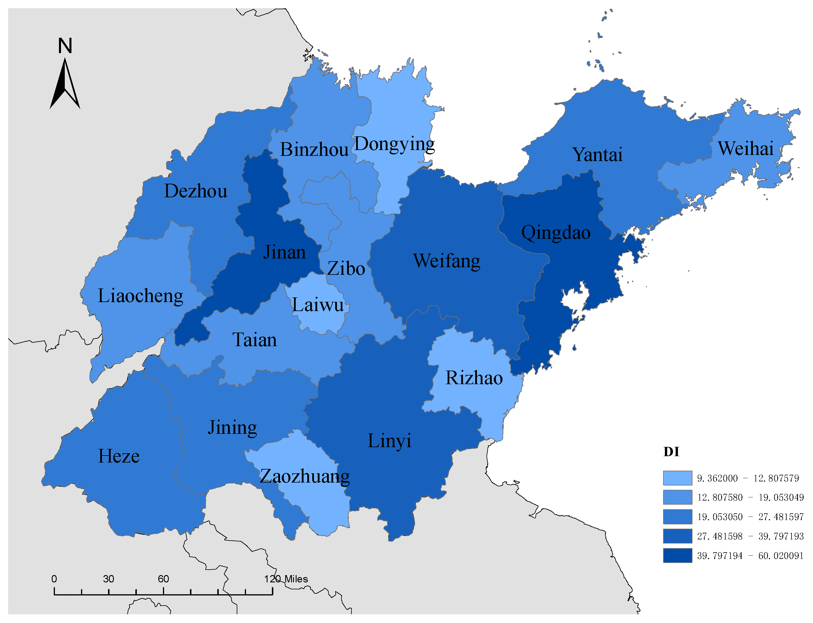
Initially, we embark on an exploration of the spatial distribution peculiarities of the Digitization Index (DI) across Shandong Province. Illustrated in Figure 2 is the territorial dissemination of DI within the province, where a gradient of darker hues signifies progressively higher digitization levels. Upon an intuitive examination, the spatial layout of DI across Shandong Province reveals no clear regularity. An apparent negative spatial spillover effect emerges, characterized by cities with elevated DI levels being typically encircled by counterparts exhibiting marginally lower DI. Moran’s I serves as an efficient analytical tool to assess spatial autocorrelation effects, with its computation delineated in Equation (8), where N is the number of cities, i and j refer to each of the cities, x is the DI index, $\overline{x}$ is the average, $w_{ij}$ is the spatial weight generated by geographic distance (discussed later), and W is the sum of all $w_{ij}$. Through the application of this formula, Moran’s I for China spanning from 2001 to 2019 consistently suggests a degree of spatial negative correlation. Figure 3 provides a visual representation of the 2019 Moran’s I, showcasing the spatial negative correlation phenomenon.

$$I={\displaystyle \frac{N{\sum }_{i=1}^N{\sum }_{j=1}^N{w}_{ij}(x_i-\overline{x})(x_j-\overline{x})}{W{\sum }_{i=1}^N{(x_i-\overline{x})}^2}}$$

(8)

Shandong Province, featuring both the provincial capital Jinan and the coastal city Qingdao as highly developed urban areas, may lead some to speculation that the observed spatial negative correlation of the Digitization Index (DI) is a result of its unique geographical characteristics rather than a genuine spatial negative correlation effect. Figure 3 clearly depicts the relationship between each city’s DI and spatial DI. Despite a modest slope, a clear linear relationship is evident for all cities’ DI in the Moran’s I graph. Although not shown here, we have also created a Moran’s I graph for the 2019 GDP, which exhibits a significantly lower degree of linear convergence compared to Figure 3. Therefore, we have grounds to believe that this spatial negative autocorrelation is inherently attributed to DI itself. This negative spatial spillover indicates that the development of the digital economy in various cities of Shandong possesses exclusivity. It should be noted that Moran’s I is merely a rudimentary approach to assessing spatial spillover. In the subsequent empirical analysis section, we will meticulously investigate the magnitude, significance, and potential causes of spatial effects.

Let us further discuss the historical development trends and patterns of the Digitization Index (DI) in Shandong Province. By calculating the weighted average based on the GDP, and then determining the weighted average of DI indices for cities within Shandong Province, Figure 4 presents Shandong’s DI and its rate of change. It is evident that from 2001 to 2019, Shandong’s DI demonstrated a clear upward trend with relatively stable growth, increasing at an approximate rate of 6.5% annually. This growth rate surpasses that of most economic indicators, such as actual GDP and population growth rates. This suggests that, after reaching a certain level of economic development and encountering specific bottlenecks, there may be a natural shift towards the development of the digital economy. It is important to note that China started to emphasize the development of the digital economy beginning in 2015 [9,19]. Thus, the historical growth pattern of the digital economy is fundamentally unaffected by policy. Moreover, research by Liubo (2022) indicates that the annual growth rate of digitization in China is about 5.7% [38]. The pace of digital economy development in Shandong Province slightly exceeds the national average. A comparison reveals that the historical trends of the digital economy indices for both Shandong Province and China are very similar, with a slight decline in 2015, followed by a significant acceleration in growth rate thereafter.

3. Empirical Analysis

In this section, we aim to explore the effects of the Digitization Index (DI) on economic development through five focused subsections. The first subsection introduces the data samples. Next, the second subsection delves into DI’s impact on GDP, examining how digitization fuels economic output. The third subsection shifts the lens to the influence of DI on Total Factor Productivity (TFP), probing into tantalization’s role in enhancing economic efficiency. The fourth subsection is dedicated to verifying the robustness and heterogeneity of our analysis, ensuring the reliability of our conclusions across various contexts. The fifth subsection investigates the spatial effects generated by DI, examining the broader implications of digitization on regional economic development.

3.1. Sample Description

In the subsequent data analysis section, information on the variables used is presented in

Table 2. Description of variables used for empirical analysis.

Variable	Name	Scale	Source
$gdp$	Gross regional product	10,000 CNY	CCSY
$work$	Number of urban employees	10,000 unit	CCSY
$inv$	Total fixed assets investment	10,000 CNY	CCSY
$cap$	Stock of fixed assets	10,000 CNY	Equations (9) and (10)
$di$	Digitization index	index	EWM method

Notes: CCSY = China City Statistical Yearbook; we use “$gdp$” for easy understanding.

. The primary source for these variables is the China City Statistical Yearbook (CCSY), which includes data on total output ($gdp$), urban labor force ($work$), and annual investment ($inv$). The Digitization Index ($di$) has already been calculated in a previous section. Therefore, the data structure consists of panel data covering 17 cities in Shandong Province in China from 2001 to 2019. Additionally, it should be noted that although total population ($pop$) and urban labor force ($work$) are both used to represent the labor force in related studies, due to the unstable population structure in China over recent decades, many demographers argue that using the urban labor force is a more accurate representation of the labor force than using total population.

The Solow residual method, which will be utilized later, necessitates data on the capital stock. Similar to related studies, the perpetual inventory method is used to calculate the fixed capital stock ($cap$) using fixed asset investment ($inv$), as illustrated in Equation (9). Equation (9) describes the computation of the capital stock of fixed assets: the stock from the previous year minus the depreciation rate multiplied by the previous stock, plus the flow from the previous year.

$$ca{p}_t=ca{p}_{t-1}-d\times ca{p}_{t-1}+in{v}_{t-1}$$

(9)

In practical application, there is a challenge in determining the initial value of the capital stock, $ca{p}_1$. It is assumed that with a constant depreciation rate and investment, the capital stock will reach a steady state, calculated as investment divided by the depreciation rate. This approach can be used to estimate the initial capital stock, shown in Equation (10). Related Research indicates that the depreciation rate in China is about 5%. So we assume that the depreciation rates of all Shandong cities are 5%. Some studies also consider constant growth rates for investment and capital, derived from the historical average growth of investment. However, this method can be overly complicated and does not reflect the actual variability in investment. Since the accuracy of the capital stock estimates improves over time using the perpetual inventory method, an extremely precise initial estimate is not crucial.

$$ca{p}_1={\displaystyle \frac{in{v}_1}{d}}$$

(10)

This paper, focusing on economic growth and the quality of economic development, retains only the two most significant factors affecting GDP: labor and capital. This approach aligns with the Cobb–Douglas production function and traditional economic growth theories, such as the Solow model. Consequently, we use $work$ to measure the impact of labor on GDP and $cap$ to assess the influence of capital on GDP.

Similar to empirical studies related to economic growth, we take the logarithms of GDP, labor ($work$), and capital ($cap$), which are represented as $lngdp$, $lnwork$, and $lncap$, respectively. The relationship between GDP and the DI is not well understood, which led us to conduct extensive preliminary regression tests. Evidence indicates a strong relationship between $lngdp$ and the logarithmic form of DI ($lndi$), as shown in Figure 5.

Figure 5 clearly illustrates a linear relationship between ln($GDP$) and ln($DI$), indicating that as $lndi$ increases, so does $lngdp$. However, given that the data are panel data, further research is required to determine whether the relationship between the two is statistically significant.

The descriptive statistics for the variables involved in the empirical section are provided in

Table 3. Calculation and statistic description of the variables.

Variable	Calculation	Obs	Mean	Std. Dev.	Min	Max
$lngdp$	=ln($gdp$)	323	16.625	0.878	14.042	18.603
$lnwork$	=ln($work$)	323	3.925	0.563	2.569	5.011
$lncap$	=ln($cap$)	323	17.587	1.316	14.297	20.213
$lndi$	=ln($di$)	323	2.452	0.642	0.614	4.095
$lntfp$	SRM	323	6.806	0.278	5.223	7.226

Notes: $lndi2=lnd{i}^2$ which is the square of $lndi$.

. The theoretical dataset comprises data from 17 cities over 19 years, totaling (17×19=) 323 observations with no missing data.

3.2. Regression Model

In this study, our sample is panel data, which necessitates the use of panel data regression models. The main types of panel data regression models are Pooled OLS, Fixed Effects (FE), and Random Effects (RE). The general form of these models is given in Equation (11). Pooled OLS regression is better when the individual effect ($u_i$) is none; FE is better when the individual effect is related to the explanatory variables and RE is better when the individual effect is unrelated to the explanatory variables.

$$Y_{it}=\alpha +\beta X_{it}+u_i+{ϵ}_{it}$$

(11)

where:

• $Y_{it}$ is the dependent variable;
• $X_{it}$ is the matrix of all explanatory variables;
• $\alpha$ is the intercept term;
• $\beta$ is the matrix of all estimated coefficients;
• $u_i$ is the individual effect (fixed or random);
• ${ϵ}_{it}$ is the residual term.

The choice between FE and RE models is determined using the Hausman test. This test checks whether the unique errors ($u_i$) are correlated with the regressors, guiding us to the most appropriate model.

To capture the spatial dependencies and interactions in our data, we employ the Spatial Durbin Model (SDM). This model is particularly useful when both the dependent variable and the explanatory variables exhibit spatial autocorrelation. The general form of the SDM is given in Equation (12).

$$Y_{it}=\rho W{Y}_{it}+\alpha +\beta X_{it}+\theta W{X}_{it}+u_i+{ϵ}_{it}$$

(12)

where:

• $Y_{it}$ is the dependent variable;
• $X_{it}$ is the matrix of all explanatory variables;
• W is the spatial weight matrix;
• $\rho$ is the spatial autoregressive coefficient;
• $\theta$ is the coefficient vector for the spatially lagged explanatory variables;
• $\alpha$ is the intercept term;
• $\beta$ is the matrix of all estimated coefficients for the explanatory variables;
• $u_i$ is the individual effect (fixed or random);
• ${ϵ}_{it}$ is the residual term.

In this model, $W{Y}_{it}$ represents the spatially lagged dependent variable, which incorporates the influence of neighboring observations’ dependent variables on the current observation. Similarly, $W{X}_{it}$ represents the spatially lagged explanatory variables, incorporating the influence of neighboring observations’ explanatory variables. By including both $\rho W{Y}_{it}$ and $\theta W{X}_{it}$, the Spatial Durbin Model allows for a more comprehensive analysis of spatial interactions and spillover effects, providing a more accurate representation of the underlying spatial processes in the data.

3.3. The Effect of DI on Economy Growth

In the baseline regression section, extensive regression analyses were conducted. The most informative results from four baseline regressions are presented in

Table 4. Results of the basic regressions.

Regression	1	2	3	4
Dependent	$\mathit{lngdp}$	$\mathit{lngdp}$	$\mathit{lngdp}$	$\mathit{lngdp}$
$lnwork$	0.370 ***		0.362 ***	0.361 ***
	(0.127)		(0.127)	(0.127)
$lncap$	0.476 ***		0.432 ***	0.423 ***
	(0.020)		(0.035)	(0.036)
$lndi$		1.695 ***	0.167	0.381 *
		(0.055)	(0.109)	(0.220)
$lndi2$				−0.037
				(0.033)
Constant	6.919 ***	12.007 ***	7.227 ***	7.092 ***
	(0.380)	(0.190)	(0.429)	(0.445)
Obs.	323	323	323	323
Reg. Model	FE	FE	FE	FE
(within) R2	0.92	0.86	0.92	0.92

Notes: (1) Standard errors are in parentheses; (2) * and *** are significant at 10% and 1% levels.

. First, ln($GDP$) is used as the dependent variable in all four regressions. Second, the fixed effect (FE) panel data regression model is chosen. This choice was guided by pre-analytical Hausman tests comparing fixed effect (FE) and random effect (RE) models, where the p-values from the Hausman test were all below 0.10, indicating that the FE model is more suitable for empirically describing and analyzing the relationships between variables.

According to economic growth theory, capital and labor are the main determinants of output, and their impacts on $lngdp$ are estimated in Regression 1. Consistent with previous research findings, both labor and capital have significant positive effects on total output.

In Regression 2, only the DI is considered as the explanatory variable, which is the focus of our study. This regression is used to check whether the total effect of DI on output is significant or not. Results indicate that $lndi$ has a significant positive impact on $lngdp$.

In Regression 3, we combined the explanatory variables from Regressions 1 and 2, namely $lnwork$, $lncap$, and $lndi$. The results show that the impacts of capital and labor on GDP remain significantly positive and are consistent with the estimators from Regression 1. However, the influence of $lndi$ on $lngdp$ becomes insignificant. According to the theory of mediation effects, these results suggest that $lndi$ has a direct impact on $lnwork$ and $lncap$, but not directly on $lngdp$. Therefore, $lndi$ is significant when labor and capital are not considered, but becomes insignificant when both are included.

In regression 4, a squared term of $lndi$ was added to test for a nonlinear relationship between $lndi$ and $lngdp$. The results indicate that the squared term of $lndi$ is not significant, suggesting that there is no significant nonlinear relationship between $lndi$ and $lngdp$.

An analysis was conducted to determine whether Regression 2 involves spurious regression.

Table 5. Panel Data Unit-Root/Stationary Test (p-value).

Test	lngdp	lndi
Levin-Lin-Chu (LLC) test	<0.001	0.831
Im-Pesaran-Shin (IPS) test	0.025	1.000
ADF-Fisher unit-root test	<0.001	0.982
Hadri LM stationary test	<0.001	<0.001

Notes: lag = 2 in ADF-Fisher unit-root test.

presents the results of stationarity tests for the panel data of $lngdp$ and $lndi$. Common tests for panel data stationarity include the LLC, IPS, ADF-Fisher, and Hadri LM tests. Each method has different null hypotheses, so the interpretations of their results vary slightly. Based on the outcomes of these tests, we are confident that $lngdp$ is stationary in the majority of panels (cities), with only a few panels (cities) showing non-stationarity; $lndi$ is non-stationary in the majority of panels (cities), with only a few cities being stationary. Given this, the probability that Regression 2 is a spurious regression is very low.

Additionally, although not directly related to the subsequent analysis, we conducted some additional tests. First, a cointegration test was performed on $lngdp$ and $lndi$. The test results indicate that there is no cointegration relationship between the two. Second, a Granger causality test was conducted between $lngdp$ and $lndi$. The results show that the p-value for $lndi$ affecting $lngdp$ is <0.001; the p-value for $lngdp$ affecting $lndi$ is 0.014. These suggest a bidirectional causality between $lngdp$ and $lndi$. The variance inflation factor (VIF) of the four regressions are also calculated to exam the multicollinearity among all the explanatory variables. The VIFs are lower than 5 in regression 1–3. The VIF of regression 4 is significantly higher than 5 since the use of the squared term.

3.4. The Effect of DI on Total Factor Productivity (TFP)

Total Factor Productivity (TFP) has increasingly become a focal point of research within the academic community, especially in recent years. This surge in interest can be attributed to the diminishing returns from traditional inputs like labor and capital in driving GDP growth. TFP measures the efficiency and effectiveness with which these inputs are utilized to produce output, capturing the impacts of technology, innovation, and improvements in organizational efficiency. As economies evolve, the role of knowledge, technology integration, and skill enhancements in stimulating economic growth has become more significant. Consequently, understanding and improving TFP is crucial for sustaining economic development, particularly in advanced economies where the potential for capital investment and workforce expansion is limited.

The Solow Residual Model (SRM) is an economic model used to measure TFP. Proposed by Nobel laureate Robert Solow, the model aims to isolate the portion of economic growth that cannot be directly attributed to inputs such as capital and labor. Within this framework, TFP is considered the “residual” factor driving output growth, encompassing the effects of technological advances and efficiency improvements that are not tied to input factors. The Solow Model underscores that long-term economic growth is primarily driven by technological changes rather than merely the accumulation of resources.

In practical applications, the Solow Residual Model enables the precise calculation of TFP as traditionally defined through Regression 1. The TFP calculated in our study is presented in logarithmic form, thus it is named $lntfp$. The descriptive statistics for $lntfp$ are provided in the last row of Table 3.

In macroeconomic studies, the input-output tables by industry are used to further distinguish capital into digital and non-digital capital. The total output of the digital sector represents digital industrialization, while the impact of digital capital on traditional industries is referred to as industrial digitization. In other words, at the national level, the digital level serves as both capital and technology, thereby directly influencing both GDP and TFP. In the context of city-level research, where input-output tables are absent, the digitization index more closely aligns with industrial digitization. As suggested by the results in Regressions 2 and 3, the digitization index does not directly impact $lngdp$, but it does indirectly influence $lngdp$ through either $lncap$ or $lnwork$. According to theories related to economic growth and TFP, the indirect effect of the digitization index on $lngdp$ should, on one hand, alter $lncap$ or $lnwork$, and on the other hand, change the marginal efficiency of $lncap$ and $lnwork$, which as a whole is TFP.

Figure 6 presents a scatter plot of ln($DI$) and ln($TFP$) from our study sample. It is evident from the plot that, aside from a few outliers in the lower middle, there is a strong positive linear relationship between $lntfp$ and $lndi$. The correlation coefficient between these variables is also calculated, which is 0.313, indicating a moderate positive correlation.

$lntfp$ is set as the dependent variable and $lndi$ is set as the independent variable, conducting a simple linear regression using Ordinary Least Squares (OLS), designated as Regression 5. below. Results confirm that $lndi$ indeed has a significant positive impact on $lntfp$. This section concludes by noting that similar findings have been reported in other related studies, reinforcing the robustness and reliability of our results.

3.5. Heterogeneity Test

In this section, a heterogeneity test is conducted. Previous evidence suggests that there may be variations among cities in Shandong Province. For instance, differences likely exist between cities in the eastern coastal areas and those in the western inland regions. Given that our research focuses on the digital economy, we categorized cities based on the DI as shown in Figure 2. Eight cities with low DI are grouped together, and nine cities with high DI are considered another group, to analyze economic growth differences based on DI levels. Similarly, we divided the entire sample period from 2001 to 2019 into two segments: 2001–2009 and 2010–2019. This division offers several advantages: each sub-period is nearly equal in length and it differentiates between the early years, when digital economy theories were not yet prevalent, and the recent period, when the digital economy has been more emphasized and developed.

In the regression model, similar to classical economic growth theory (Regression 1), $lngdp$ is used as the dependent variable, with $lnwork$ and $lncap$ as the explanatory variables. Regarding the regression method, we opted for OLS instead of FE because individual effects might inherently vary in size between groups prior to categorization, which could lead to misjudgment when assessing differences between groups. Consequently, in

Table 6. Results of the conditional regressions.

Regression	6	7	8	9	10
Dependent	$\mathit{lngdp}$	$\mathit{lngdp}$	$\mathit{lngdp}$	$\mathit{lngdp}$	$\mathit{lngdp}$
$lnwork$	0.581 ***	0.595 ***	0.646 ***	0.518 ***	0.714 ***
	(0.032)	(0.075)	(0.058)	(0.031)	(0.067)
$lncap$	0.456 ***	0.446 ***	0.451 ***	0.524 ***	0.307 ***
	(0.014)	(0.023)	(0.019)	(0.016)	(0.052)
Constant	6.334 ***	6.467 ***	6.120 ***	5.431 ***	8.537 ***
	(0.194)	(0.316)	(0.255)	(0.226)	(0.802)
Obs.	323	133	190	170	153
Reg. Model	OLS	OLS	OLS	OLS	OLS
Region	All	low DI	high DI	All	All
Time	2001–2019	2001–2019	2001–2019	2001–2009	2010–2019
(within) R2	0.91	0.89	0.91	0.95	0.76

Notes: (1) Standard errors are in parentheses; (2) *** is significant at 1% level.

, Regression 6 represents the regression for the full sample, while Regressions 7 and 8 are grouped regressions analyzing regional DI differences. Regressions 9 and 10 are grouped regressions reflecting temporal differences.

Comparing the regression results from Regressions 7 and 8 in Table 6, the estimators for both $lnwork$ and $lncap$ are almost the same but relatively high in regions with high DI. This implies that there is no significant regional difference and also indirectly indicates that cities with higher DI possess relatively higher TFP, resulting in greater marginal returns to capital and labor.

Comparing the results of Regressions 9 and 10 in Table 6, the estimator for $lnwork$ is notably higher in the recent period, coinciding with the development of the digital economy. This aligns with our theoretical deductions that as the digital economy progresses, the human capital of the workforce significantly increases along with their work efficiency. However, the estimator for $lncap$ has decreased markedly in the same period. Theoretically, as the digital economy expands, including digital finance, the ease of capital flow should enhance the marginal efficiency of capital. Upon reflection and discussion, it was realized that our chosen proxy for capital, based on the “Stock of fixed assets” from the China City Statistical Yearbook, overlooks the issue of virtual capital. As we know, with the growth of the digital economy, non-tangible assets such as digital currencies have also flourished. Therefore, the contrasting results of Regressions 9 and 10 should not be interpreted as a decline in capital’s marginal efficiency on GDP, and this issue warrants further investigation.

3.6. The Spatial Effect of DI

In spatial econometrics, spatial effects refer to the influence that variables within one geographical area can exert on the same or related variables in neighboring areas. This concept highlights the interconnectedness and the potential spillover effects between regions, where changes in one locale can ripple through to others. In the context of this study, it means that the DI in one area not only affects its own GDP but also has implications for the GDP in other regions. Similarly, the DI from neighboring regions can influence local economic performance. This analysis is particularly vital for understanding the dynamics of economic development and its sustainability, as spatial analysis helps us capture both direct and indirect impacts of digital advancements across different regions.

From a data analysis perspective, Figure 3 and the associated Moran’s I provide clear evidence of the presence of negative spatial spillover effects. Therefore, it is necessary to further investigate using spatial econometric models to analyze (i) whether spatial effects exist and (ii) whether these spatial effects impact the effects of the variables.

Spatial econometric models are pivotal for analyzing data that exhibit spatial interdependence and autocorrelation among variables across regions. The primary models include the Spatial Autoregression (SAR) model, which addresses the influence of a region’s dependent variable on its neighbors; the Spatial Error Model (SEM), which corrects for autocorrelation in the errors; the Spatial Durbin Model (SDM), which extends SAR by including lagged independent variables of neighboring regions. In this study, we utilize the Spatial Durbin Model (SDM) due to its capability to comprehensively assess both the direct and indirect effects of variables, such as DI on economic performance (GDP and TFP), thus providing a deeper insight into the spatial dynamics influencing regional economic development.

The spatial weight matrix is a fundamental component in spatial econometric analysis, used to define the spatial relationships between observations. It specifies how much influence one region exerts on another, which is crucial for models that account for spatial interactions. In this study, we utilize two types of spatial weight matrices: W1 and W2. W1 is an adjacency matrix, defining spatial connections based on direct neighboring relationships. W2, on the other hand, is a geographic distance matrix calculated based on latitude and longitude coordinates. Given that Shandong Province is relatively small in size, it is not necessary to consider the distortions in distance measurements that might be caused by the spherical shape of the Earth, simplifying the calculation and use of geographic distances in our analysis.

It is important to clarify that in setting the explanatory variables for our model, we conducted preliminary regression tests. The results indicated that capital, labor, and DI can be used simultaneously as explanatory variables. We constructed Regression 11 and Regression 12, which differ in their use of spatial weight matrices W1 and W2, respectively.

Table 7. Spatial effect of $lndi$ on $lngdp$.

Regression	11	12	Regression	11	12
Dependent	$\mathit{lngdp}$	$\mathit{lngdp}$	Dependent	$\mathit{lngdp}$	$\mathit{lngdp}$
$lnwork$	0.259 *	0.212 *	(The long-
	(0.150)	(0.126)	run effects)
$lncap$	0.040	0.009	Direct: $lnwork$	0.281 *	0.224 *
	(0.041)	(0.043)		(0.146)	(0.129)
$lndi$	0.215 ***	0.247 ***	Direct: $lncap$	0.080 **	0.039
	(0.071)	(0.071)		(0.039)	(0.042)
Constant	1.843 ***	1.085 **	Direct: $lndi$	0.217 ***	0.218 ***
	(0.401)	(0.426)		(0.083)	(0.081)
Wx: $lnwork$	−0.129	-0.141	Indir.: $lnwork$	0.155	0.125
	(0.174)	(0.162)		(0.308)	(0.495)
Wx: $lncap$	0.097 **	0.122 *	Indir.: $lncap$	0.377 ***	0.598 ***
	(0.048)	(0.063)		(0.102)	(0.220)
Wx: $lndi$	−0.168 *	−0.344 **	Indir.: $lndi$	−0.053	−0.690
	(0.100)	(0.150)		(0.307)	(0.665)
Spatial: $\rho$	0.701 ***	0.794 ***
	(0.037)	(0.034)
Obs.	323	323
S.W. matrix	W1	W2
Reg. Model	SDM	SDM
Fixed effect	individual	individual
(within) R2	0.81	0.79

Notes: (1) Standard errors are in parentheses; (2) *, **, *** are significant at 10%, 5% and 1% levels; (3) Results of Hausman tests suggest exclusion of time fixed effect.

presents the results of Regression 11 and 12. The table is divided into two sections: the left side displays the main body of the two regressions, while the right side details the direct and indirect long-term effects. It is particularly worth noting that in regressions 11 and 12, the time-fixed effects were found to be insignificant according to the Hausman test. Consequently, the model specification includes only individual fixed effects. In contrast to the previous models, this specification considers only spatial effects, which themselves do not include time lags. The insignificance of time-fixed effects may be attributed to the similarity in temporal trends across regions, implying that local time-fixed effects are largely explained by the surrounding areas. The regression results for Regression 11 and 12 are extremely similar in terms of their signs and significance, which indirectly suggests that spatial effects are predominantly driven by geographic distance. The adjacency of the two regions does not have a significant impact.

For Regression 12, results show that locally, both labor and DI have a significant positive impact on GDP, whereas the effect of capital is not significant. Regarding spatial effects, the capital of surrounding cities has a significant positive impact on local GDP, aligning with the boundary-less nature of capital flows; however, this is not the main focus of our study and will not be analyzed extensively. Most importantly, spatial effects also reveal that the DI of surrounding areas has a significant negative impact on local GDP. In other words, a higher DI in surrounding areas suppresses local economic development; conversely, robust local DI development can inhibit the GDP growth of neighboring cities. The reasons for this spatial suppressive effect of DI require further analysis.

Based on the findings mentioned earlier, the negative spatial spillover effect of DI on GDP is likely mediated by a direct impact of DI on TFP, which in turn indirectly affects GDP. Therefore, we constructed Regression 13 and 14, with $lntfp$ as the dependent variable and $lndi$ as the explanatory variable, using two different spatial weight matrices, W1 and W2, as shown in

Table 8. Results of further spatial regressions.

Regression	5	13	14	15	16
Dependent	$\mathit{lntfp}$	$\mathit{lntfp}$	$\mathit{lntfp}$	$\mathit{lndi}$	$\mathit{lndi}$
$lndi$	0.135 ***	0.138 ***	0.146 ***
	(0.023)	(0.033)	(0.033)
Spatial: $\rho$		0.587 ***	0.732 ***
		(0.045)	(0.043)
Wx: $lndi$		−0.083 **	−0.134 ***	−0.114 *	−0.829 ***
		(0.040)	(0.043)	(0.070)	(0.204)
Constant	6.474 ***	2.670 ***	1.792 ***	2.140 ***	3.456 ***
	(0.058)	(0.321)	(0.299)	(0.196)	(0.402)
Direct: $lndi$		0.139 ***	0.143 ***
		(0.034)	(0.034)
Indirect: $lndi$		0.005	−0.085
		(0.070)	(0.114)
Obs.	323	323	323	323	323
S.W. matrix	-	W1	W2	W1	W2
Reg. Model	OLS	SDM	SDM	SAR	SAR
(within) R2	0.10	0.10	0.12	0.25	0.25

Notes: (1) Standard errors are in parentheses; (2) *, **, *** are significant at 10%, 5% and 1% levels; (3) $\rho$ is the estimator of SAR model, they are removed to Wx: $lndi$ for comparison.

. The results indicate a significant negative spatial spillover effect of DI on TFP. In other words, an increase in DI in surrounding areas leads to a decline in local TFP, or an increase in local DI causes a decline in TFP in neighboring areas. Although this outcome suggests that the spatial effect of DI on GDP operates through TFP, the negative spatial spillover effect remains economically challenging to interpret.

We hypothesize that local DI may have a spatial effect on the DI of surrounding areas, thereby impacting the TFP of these regions. Consequently, we constructed Regression 15 and 16, where the dependent variable is local DI and the explanatory variable is DI from surrounding areas, using two different spatial weight matrices, W1 and W2. Due to the absence of other explanatory variables, we could not employ the SDM and instead opted for the Spatial Auto-Regressive (SAR) model for regression analysis, with results presented in Table 8. The findings confirm a significant negative spatial spillover effect of DI. This suggests that when DI in surrounding areas is robust, local DI tends to grow slowly; conversely, strong local DI development can suppress DI growth in neighboring areas. Therefore, the mechanism of influence is characterized by a significant negative spatial effect of DI, leading to significant negative spatial spillover effects on both TFP and GDP.

The underlying causes or mechanisms of the negative spatial spillover effects of DI are significant issues. However, due to the complexity of these issues and the limitations of space, they will be further researched in the future. Through our discussion, we support and believe that both economic and policy factors play a role in the development of negative spatial spillover effects of DI. For example, at the outset, national or local governments are more likely to invest in provincial capital cities like Jinan, having established facilities such as the National Supercomputer Center and the Jinan Artificial Intelligence Computing Center (AICC). If surrounding cities require digital economic capital or services, they are more likely to purchase resources from Jinan. In this scenario, the digitization level in Jinan may exceed its actual level, while the digitization in surrounding areas likely falls below their actual needs. This typical leader-follower pattern is one of the causes of negative spatial spillover. While this mode of concentrating resources in central cities to drive regional development may be more effective in terms of input-output in building a digital economy, but it is likely ineffective in terms of its impact on production efficiency, economic development, regional balanced development, and sustainability.

4. Discussion

In this section, we will first compare the theoretical inferences and empirical results of this study with those in related research. Following this, we will discuss policy recommendations. Finally, we will outline the limitations of this study and suggest directions for future research.

4.1. Comparison with Previous Studies

This study focuses on the regional level, in contrast to most related research conducted at the national level. Our findings indicate that the Digitization Index (DI) directly enhances Total Factor Productivity (TFP) and indirectly promotes GDP growth. This aligns with some existing literature. For instance, Bai et al. (2022) pointed out that the development of the digital economy facilitates industrial structure transformation [32]. Their research emphasizes the critical role of digital technology in upgrading traditional industries and fostering emerging industries, which resonates with our observation of DI’s positive impact on TFP. Similarly, Cai and Niu (2021) found that the value-added of the digital economy significantly promotes regional economic growth [33]. Their study particularly highlights the contribution of the digital economy to improving production efficiency and innovation capacity, consistent with our finding that DI indirectly boosts GDP growth.

Our study, however, reveals significant negative spatial spillover effects of DI, indicating that high digitization levels in one area may suppress economic development in neighboring regions. This finding is in line with Li et al. (2023), who noted spatial heterogeneity in the impact of the digital economy on regional green development [34]. Li et al.’s research underscores the regional imbalance in digital economic development, which contrasts interestingly with our observed spatial spillover effects.

Additionally, our results echo the findings of Zhang et al. (2021) [37]. They investigated the impact of the digital economy on high-quality economic development in China, discovering that the digital economy not only directly promotes economic growth but also indirectly drives it by enhancing innovation capacity and resource allocation efficiency. This is consistent with our conclusion that DI indirectly influences GDP by improving TFP.

It is noteworthy that our methodological approach differs from that of Liu and Hong (2022) [38]. They proposed analyzing the digital economy by dividing it into digital industrialization and industrial digitization. Although our study did not make such distinctions, this approach offers a valuable perspective for future research, potentially aiding in a more precise understanding of the digital economy’s impact on different economic sectors.

4.2. Policy Recommendations

Based on our research findings, we propose the following four policy recommendations:

First, enhancing production efficiency and GDP. The government can improve production efficiency and GDP through the development of the digital economy. The advancement of the digital economy can provide various conveniences in daily life and business operations, accelerating communication, payment, and information transmission, thereby directly enhancing production efficiency and indirectly promoting GDP growth. For example, the promotion of high-speed broadband and 5G networks can significantly increase information transmission speeds, fostering the development of e-commerce and smart manufacturing.

Second, developing differentiated. In the initial stages of building the digital economy, it is necessary to implement differentiated development across various regions. This differentiation should primarily focus on the direction of digital development, tailored to each city’s strengths, such as administrative importance for provincial capitals, tourism for cities with natural attractions, or cultural heritage for historically significant cities.

Third, promoting the digital economy. The outcomes of the digital economy need to be realized through people’s learning and use of related products to demonstrate their true value. Governments can enhance public awareness and the adoption of digital technologies through organized training sessions, seminars, and promotional activities. Additionally, businesses should actively participate by developing user-friendly digital products and services, lowering the barriers to user adoption.

Fourth, balancing regional development. The development of the digital economy should be balanced across different regions. Promoting balanced development across regions, with complementary digital strengths, will contribute to sustainable economic growth. For instance, the government can use fiscal transfers and policy support to help underdeveloped regions build digital infrastructure, thereby narrowing the digital divide. Simultaneously, encouraging cooperation between developed and underdeveloped regions can facilitate the sharing of the benefits of digital economic development.

4.3. Limitations and Future Research

Despite providing valuable insights, our study has several limitations and suggests directions for future research:

(1) The dynamic effects. Although we employed dynamic panel models and Panel-VAR regression to investigate dynamic effects, the results were not significant. Thus, we believe that the impact of digital technology on the economy differs from that of other technologies. Our data suggest that DI does not exhibit the same clear dynamic effects as technology, although theoretically, DI should. We suspect that the accumulation of DI, similar to human capital such as education, may require a longer time to take effect. The issue of DI’s dynamic effects is complex and warrants further exploration. Future research could consider using data over a longer time span or adopting more refined dynamic models to capture the long-term effects of DI.

(2) The spatial effects. In studying spatial effects, this research did not consider the influence of areas surrounding Shandong Province, such as Beijing, hence the research needs further refinement. Future studies could expand to a larger geographical scope, considering the development of the digital economy in neighboring provinces and the interactions between these regions. Additionally, spatial econometric methods could be employed to analyze the spatial spillover effects of the digital economy more deeply.

(3) The spatial exclusivity. Most importantly, DI exhibits inherent spatial exclusivity, but the reasons behind this phenomenon remain unclear. It is necessary to investigate whether this phenomenon is unique to Shandong, characteristic of China or a global occurrence. Moreover, whether this exclusivity naturally arises from economic laws or results from policy influences and national planning also remains unclear and merits deeper analysis. Future research could conduct cross-country comparisons to explore the digital economy development patterns in different countries and regions and their impact on spatial exclusivity.

(4) Data Limitations. The data for this study primarily come from the China City Statistical Yearbook. While the data are relatively comprehensive, there are still some limitations. For example, the time span of the data is limited, making it difficult to capture long-term trends. Additionally, the lack of data on some key variables (such as virtual capital) may affect the accuracy of the research results. Future research could attempt to obtain more diversified and high-quality data to improve the reliability and validity of the study.

5. Conclusions

In conclusion, this study examined the impact of the digital economy on economic development in Shandong Province, an essential area that reflects the broader economic dynamics of China. We utilized annual panel data from 2001 to 2019 for the 17 cities in Shandong and developed a digitization index (DI) through the entropy weight method. Using various regression models, including fixed effects and spatial regressions, we analyzed the effects of DI on GDP and total factor productivity (TFP). Our findings indicate that DI directly enhances TFP and indirectly boosts GDP. The analysis also revealed significant negative spatial spillover effects of DI, suggesting that high levels of digitization in one area could suppress economic development in neighboring areas. Based on these insights, we recommend that the government should not only continue to vigorously develop the digital economy but also ensure an equitable distribution of digital resources across different regions. This approach should guide the development of a digital economy with regional characteristics. This balanced approach is crucial for promoting sustainable economic growth and equitable development throughout the province.