Advancing Spatiotemporal Pollutant Dispersion Forecasting with an Integrated Deep Learning Framework for Crucial Information Capture

Abstract

This study addressed the limitations of traditional methods in predicting air pollution dispersion, which include restrictions in handling spatiotemporal dynamics, unbalanced feature importance, and data scarcity. To overcome these challenges, this research introduces a novel deep learning-based model, SAResNet-TCN, which integrates the strengths of a Residual Neural Network (ResNet) and a Temporal Convolutional Network (TCN). This fusion is designed to effectively capture the spatiotemporal characteristics and temporal correlations within pollutant dispersion data. The incorporation of a sparse attention (SA) mechanism further refines the model’s focus on critical information, thereby improving efficiency. Furthermore, this study employed a Time-Series Generative Adversarial Network (TimeGAN) to augment the dataset, thereby improving the generalisability of the model. In rigorous ablation and comparison experiments, the SAResNet-TCN model demonstrated significant advances in predicting pollutant dispersion patterns, including accurate predictions of concentration peaks and trends. These results were enhanced by a global sensitivity analysis (GSA) and an additive-by-addition approach, which identified the optimal combination of input variables for different scenarios by examining their impact on the model’s performance. This study also included visual representations of the maximum downwind hazardous distance (MDH-distance) for pollutants, validated against the Prairie Grass Project Release 31, with the Protective Action Criteria (PAC) and Immediately Dangerous to Life or Health (IDLH) levels serving as hazard thresholds. This comprehensive approach to contaminant dispersion prediction aims to provide an innovative and practical solution for environmental hazard prediction and management.

1. Introduction

The rapid development of industrialisation and urbanisation has led to an increased focus on the dispersion of atmospheric pollutants as a key research topic in the field of environmental sustainability [1,2]. The dispersion of pollutants exhibits dynamic complexity in time and space and is influenced by a variety of interrelated factors. For instance, the formation of a night-time inversion layer or the occurrence of storms can lead to rapid and non-stationary fluctuations in pollutant dispersion. The intricacy of these challenges renders it challenging to adapt conventional dispersion prediction techniques to this intricate scenario, compelling researchers to pursue novel methodologies and strategies to surmount the constraints of the conventional paradigm [3,4].

Deep learning models help to better understand pollutant dispersion patterns by analysing and extracting temporal relationships and spatial trends, providing valuable predictive and decision support [5,6]. Previous studies have used Convolution Neural Networks (CNNs) to extract spatial information from pollutant dispersion data and Recurrent Neural Networks (RNNs) to discover temporal correlations between data [7,8,9]. However, these models still have some limitations. For example, CNNs may lose edge and detail information when processing high-dimensional data, which is unacceptable for representing fine-scale variations in pollutant dispersion [10,11,12]. Conversely, RNNs are prone to the problem of gradient vanishing or gradient explosion when dealing with long sequential data, which affects the ability of the models to capture complex temporal dependencies [13,14,15]. Therefore, there is a need to develop new modelling approaches to overcome these limitations and improve the accuracy and reliability of predictions.

In this study, we proposed a deep learning architecture incorporating a Residual Neural Network (ResNet) and a Temporal Convolutional Network (TCN), called SAResNet-TCN, which aims to adequately capture the spatial and temporal features of pollutant dispersion. ResNet solves the degradation problem in training deep CNNs by introducing residual learning, which allows the network to learn a deeper representation of the features [16,17]. With residual connectivity, the model effectively avoids information loss when training deep models and mitigates the problem of gradient vanishing [18,19]. In contrast, a TCN effectively captures long-term dependencies in sequence data while maintaining temporal consistency by introducing a causal convolution and diffusion layer structure [9,14]. When ResNet is combined with a TCN, a more comprehensive feature representation and modelling capability can be created, enhancing the model’s ability to represent complex patterns and improving prediction accuracy. In addition, a sparse attention (SA) mechanism was specifically incorporated in this study to take advantage of the sparsity that it introduces to strengthen the model’s focus on key features in time-series data [20]. This strategy greatly improves the sensitivity of the model to key temporal nodes and features in the prediction of pollutant dispersion peaks, providing strong support for accurate prediction. These advantages enable SAResNet-TCN to predict pollutant dispersion patterns, especially the unconventional dispersion behaviours caused by unexpected events.

The main contributions of this study can be summarised as follows:

1. An innovative deep learning model named SAResNet-TCN is introduced. This model is uniquely designed with an attention branch that operates in parallel with ResNet to extract and integrate key features, thereby enhancing the model’s ability to identify and capture significant features. In addition, the integration of the TCN module ensures that the model effectively captures the temporal dependencies between features. Validated through case studies, the proposed model demonstrated improved accuracy in predicting pollutant dispersion, providing a novel approach to support environmental sustainability.

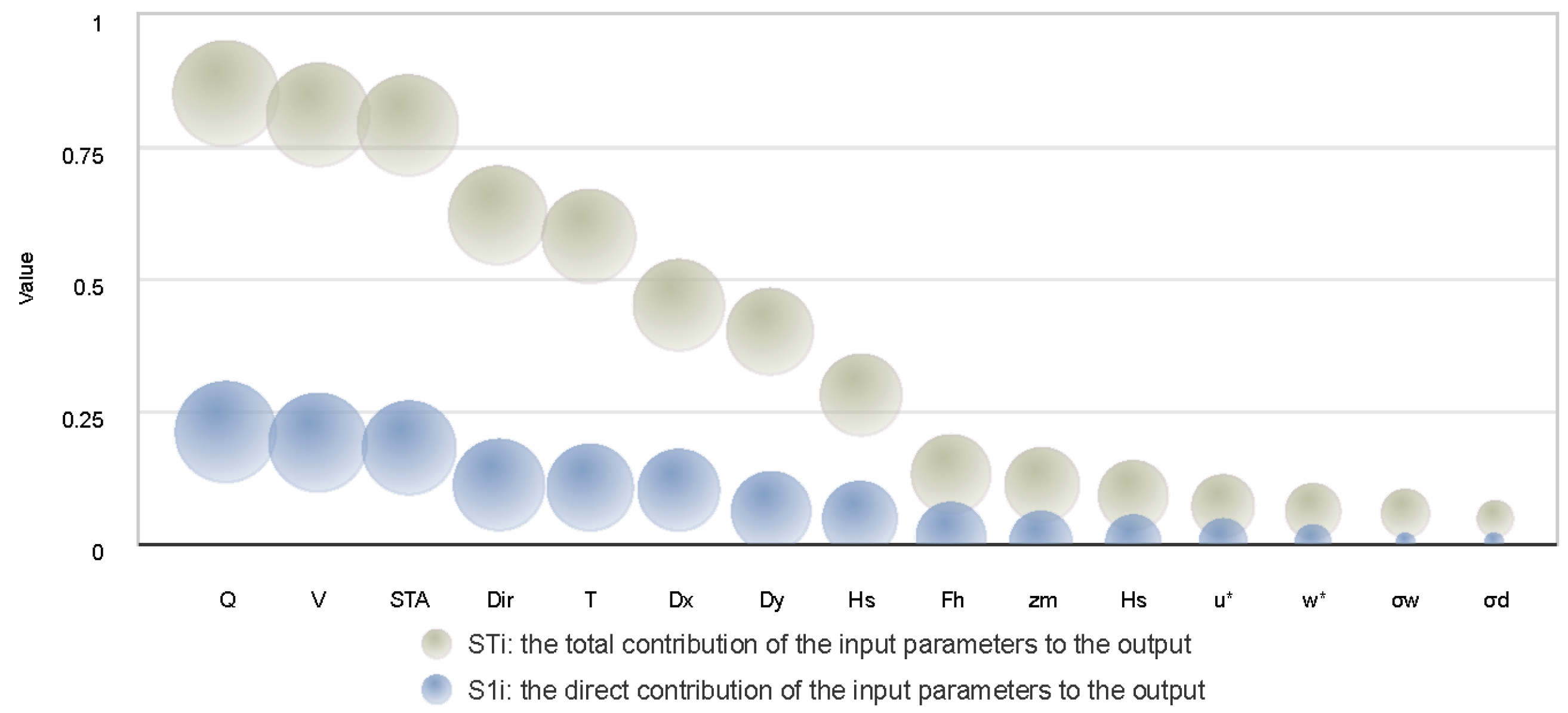
2. A global sensitivity analysis (GSA) was used to improve the interpretability and practical value of deep learning models in environmental management. Using the Sobol method, the impact of input parameters on model outputs was quantitatively analysed, identifying factors such as wind speed, atmospheric stability level, and pollution source strength as dominant influences on pollutant dispersion. Through the incremental addition of parameters into the experiments, this study further identified the key parameters that should be prioritised in resource-constrained scenarios and provides recommendations for effective resource allocation.

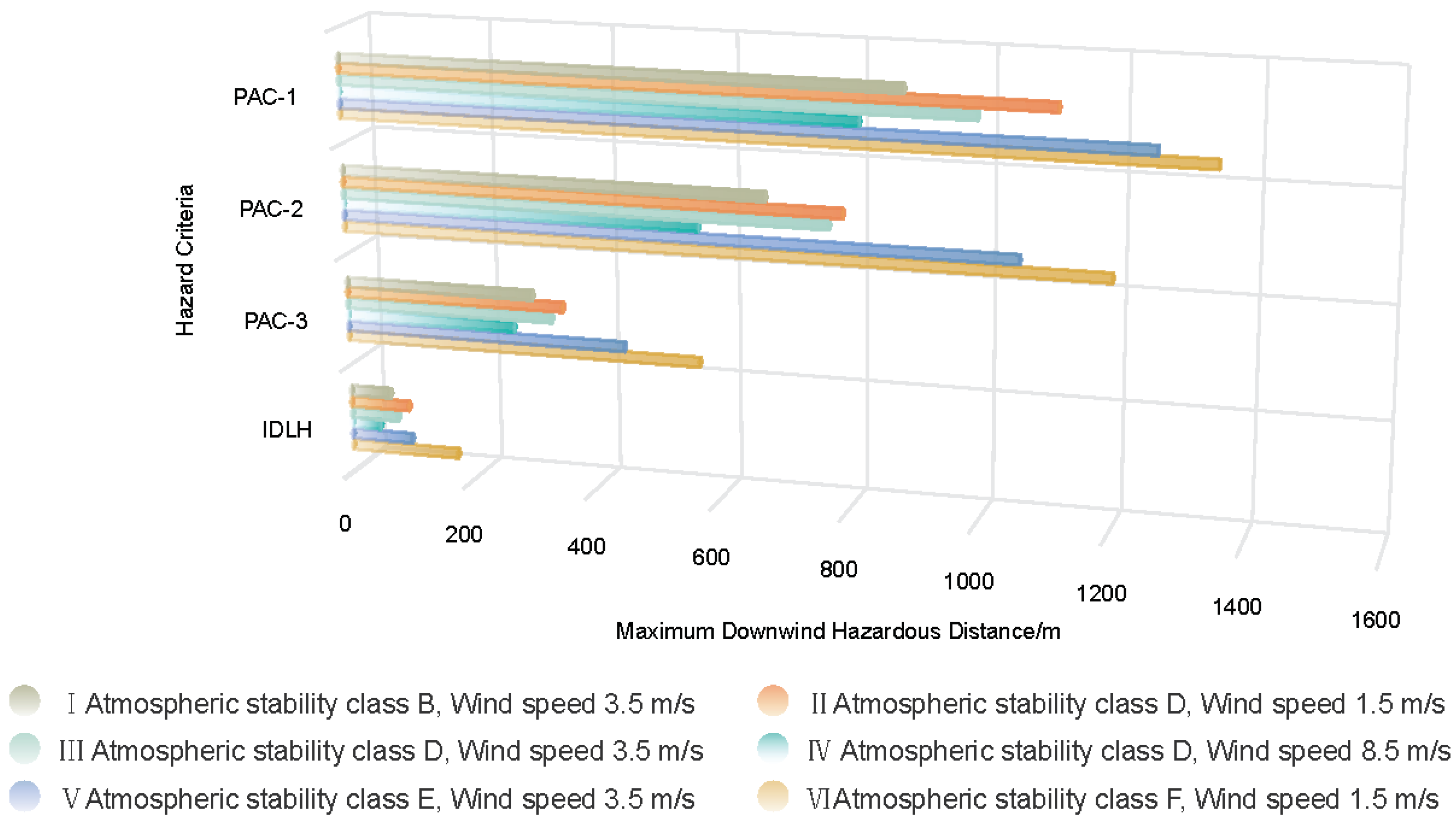
3. By applying standards such as the Protective Action Criteria (PAC) and Immediately Dangerous to Life or Health (IDLH) values, the maximum distances to hazard (MDH-distances) were visualised at different sulphur dioxide (SO₂) concentration hazard thresholds according to the six weather conditions defined in GBT37243-2019 [21]. The results not only help to assess the serious consequences of uncontrolled toxic releases but also provide an important basis for worker protection in industrial environments.

This paper is organised as follows: Section 2 outlines the specific details of the proposed pollutant dispersion prediction model. Section 3 presents the experimental results and describes the results for different hazard thresholds. Finally, the main conclusions of this study are summarised in Section 4.

2. Methodology and Proposed Model

2.1. Methods

2.1.1. ResNet

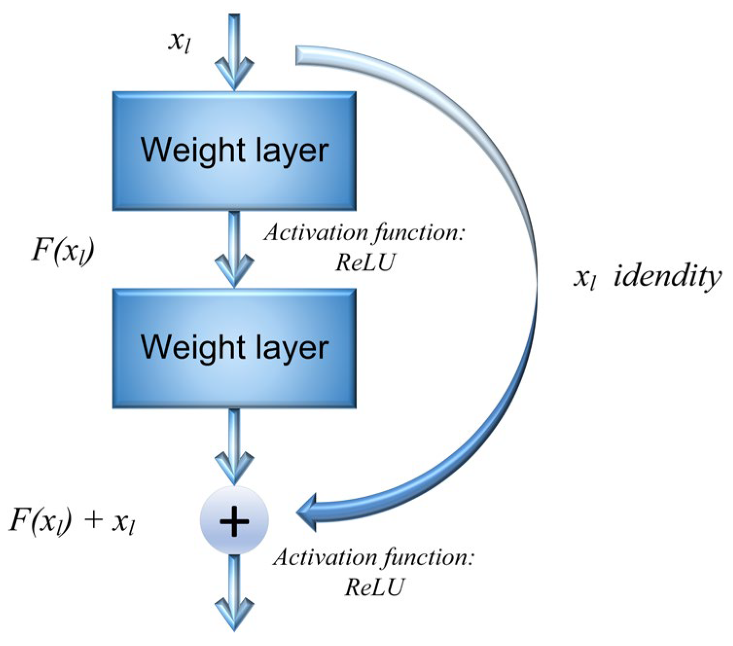
When tackling the task of pollutant dispersion modelling, ResNet uses convolution kernels to capture the distribution of pollutant concentrations in a local area and identify local concentration variations and spatial relationships. This local perceptivity allows ResNet to effectively capture the local characteristics of pollutant dispersion, thereby improving the accuracy of the model. Compared to a CNN, ResNet incorporates residual connections. This structure boosts the network’s propagation efficiency by combining residual units with directly connected edges. Thus, the model’s loss of original information is significantly reduced [22]. ResNet is composed of basic residual blocks, as shown in Figure 1. Each basic residual block comprises a mapping section and a residual section, with the core formula shown in Equation (1).

$$x_{l+1}=x_l+F\left(x_l+W_l\right)$$

(1)

In the formula, $x_{l+1}$ and $x_l$ are the feature inputs of the l + 1th and lth layers of the model, respectively; $W_l$ refers to the weight parameters of the residual cells.

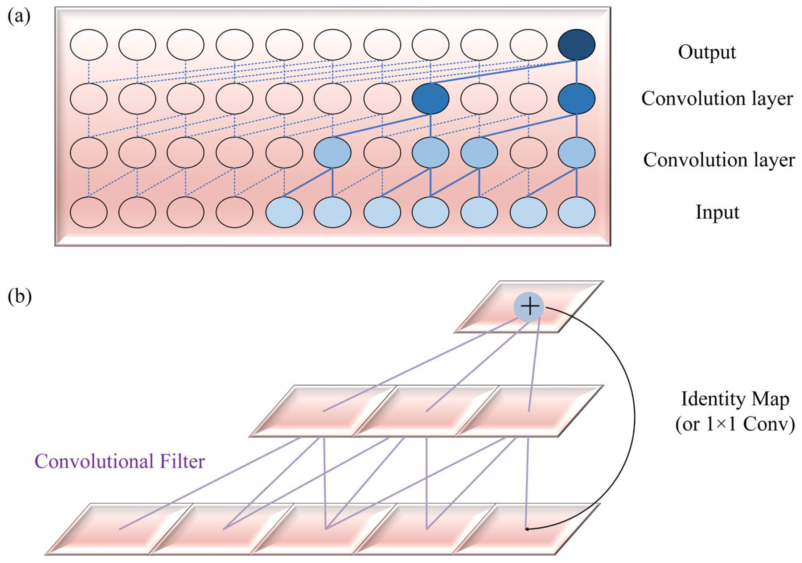
2.1.2. TCN

A TCN possesses superior time-series data processing capabilities and has demonstrated better performance than LSTM and GRU [23,24]. The fundamental elements of a TCN comprise dilated causal convolution and residual concatenation. Dilation causal convolution introduces both causality and dilation. By incorporating dilation into the convolutional kernel, dilation causal convolution can widen the receptive field of the kernel without sacrificing causality, thereby capturing a greater amount of contextual information. This technique is highly valuable for handling time-series data, permitting the TCN to model long-term dependencies effectively while maintaining causality. Residual connectivity serves the purpose of mitigating the issue of gradient vanishing while augmenting the flow of information through the network. Furthermore, it encourages the stability of the training process, allowing the network to acquire complex feature representations at a deeper level [25]. Please refer to Figure 2 for a diagram of the basic modules of a TCN.

2.1.3. SA Mechanism

The roots of attentional mechanisms can be traced back to the examination of human cognitive processes and explorations in neuroscience. Early attention mechanisms played an important role in deep learning by allowing models to selectively focus on specific information while processing input [26,27]. Nonetheless, traditional attention mechanisms generally have a global scope that assigns attention weights to all elements in the input. As a result, the computational and storage requirements are substantial [28]. The recently proposed SA mechanism, however, improves the traditional attention mechanism by introducing sparsity, which significantly reduces the time complexity [29]. The calculation formula is displayed in Equation (2). The SA mechanism allows the model to prioritise task-relevant key information and disregard irrelevant elements by selectively assigning attention weights. This precise allocation of attention improves the model’s efficiency and scalability while mitigating the risk of overfitting [29,30].

$$SparseAttention=softmax\left(\frac{\overline{Q}{K}^T}{\sqrt{d}}\right)V$$

(2)

where K and V represent the key matrix and the value matrix; $\overline{Q}$ denotes the sparse matrix; d represents the dimension of $Q$; and T stands for the transpose operation of the matrix.

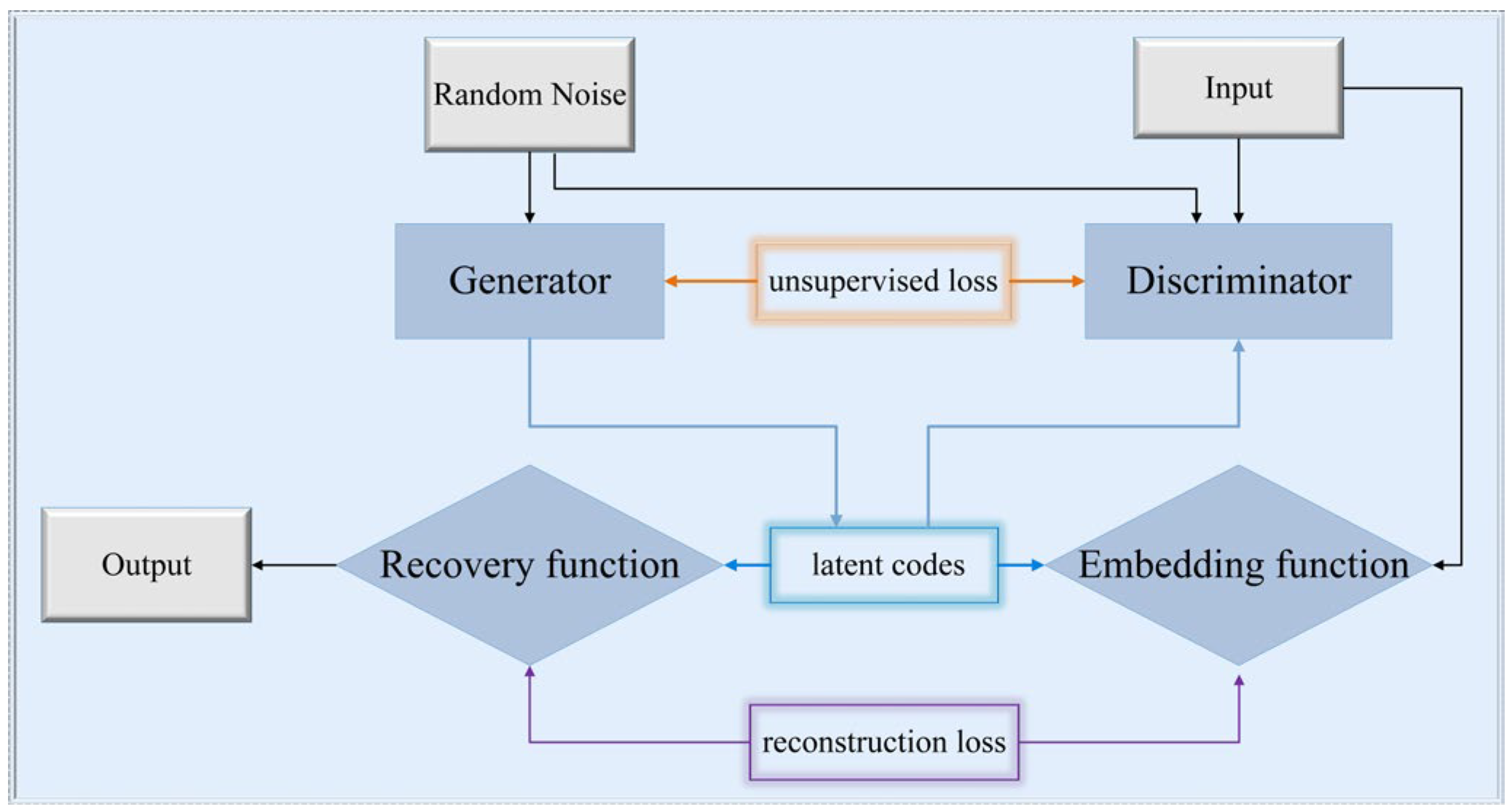
2.1.4. TimeGAN

TimeGAN is a Generative Adversarial Network (GAN) variant that combines the flexibility of unsupervised learning with the precise control of supervised learning, allowing for finer-grained dynamic tuning of the network [31]. In the standard GAN framework, the core component is an adversarial module consisting of two networks: a generator and a discriminator [32]. Through adversarial training between the generator and the discriminator, the GAN can continuously improve the data generated by the generator, making it increasingly more realistic, while at the same time improving the ability of the discriminator to discriminate between real and generated data.

TimeGAN not only contains the adversarial module of the traditional GAN but also adds a self-coding module [15]. The main function of this self-coding module is to perform dimensionality reduction on the data. It consists of two parts, namely, an embedding function and a recovery function, which are connected by latent codes. The embedding function uses the hidden function to convert the data into a low-dimensional representation, and then the data are sent to the discriminator for screening. After screening by the discriminator, the data are inversely transformed by the recovery function to produce an enhanced dataset. To introduce time-series relationships between the data in the GAN network, TimeGAN uses a supervised loss function based on an autoregressive learning algorithm. This allows the network to learn and model time-dependent probabilities, which, in turn, generates data with time-series properties [33]. Figure 3 shows how data are processed and generated by the different modules of the network in TimeGAN.

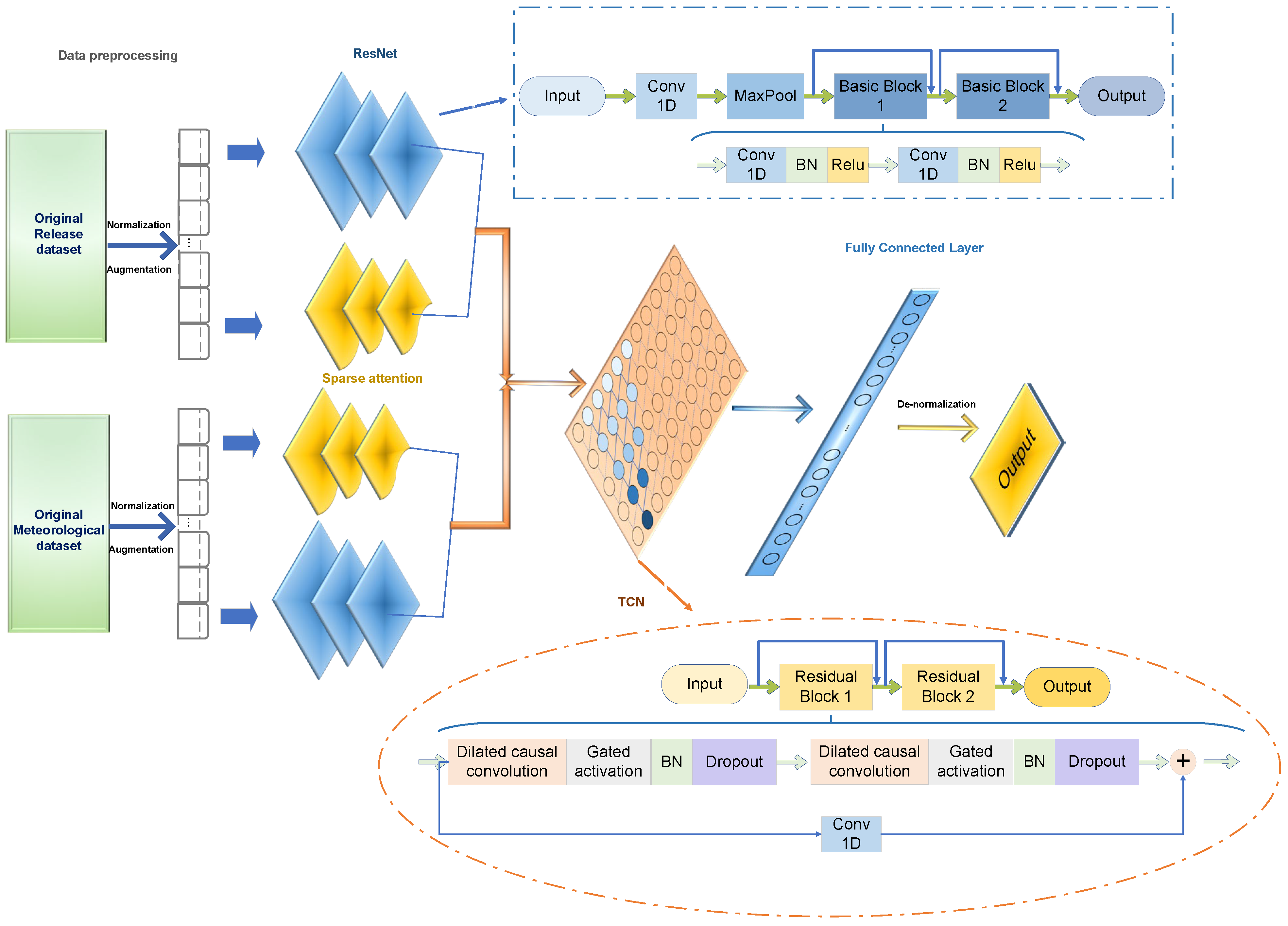
2.2. The Proposed Model: SAResNet-TCN

Figure 4 depicts the SAResNet-TCN framework, followed by a sequential explanation of its fundamental stages.

(1)

Data Preprocessing

In the construction of deep learning models, the diversity of the dataset, which may include a variety of data types, can cause higher numerical features to have a more significant influence on the model, while the influence of features with lower numerical values is reduced. To address this issue, this study used the min–max normalisation method in the data preprocessing stage. This method effectively scales or transforms the data and reduces the scale differences between features, thereby improving the generalisation ability of the model to new data and helping to mitigate the phenomenon of overfitting. The calculation formula for this method is shown in Equation (3).

$$x_{normal}=\frac{x-x_{\min }}{x_{\max }-x_{\min }}$$

(3)

In the equation, $x_{normal}$ is the value obtained after normalisation; $x$ represents the data to be normalised; $x_{\mathrm{m}\mathrm{i}\mathrm{n}}$ is the minimum value in the data; and $x_{\mathrm{m}\mathrm{a}\mathrm{x}}$ is the maximum value in the data.

(2)

Data Augmentation

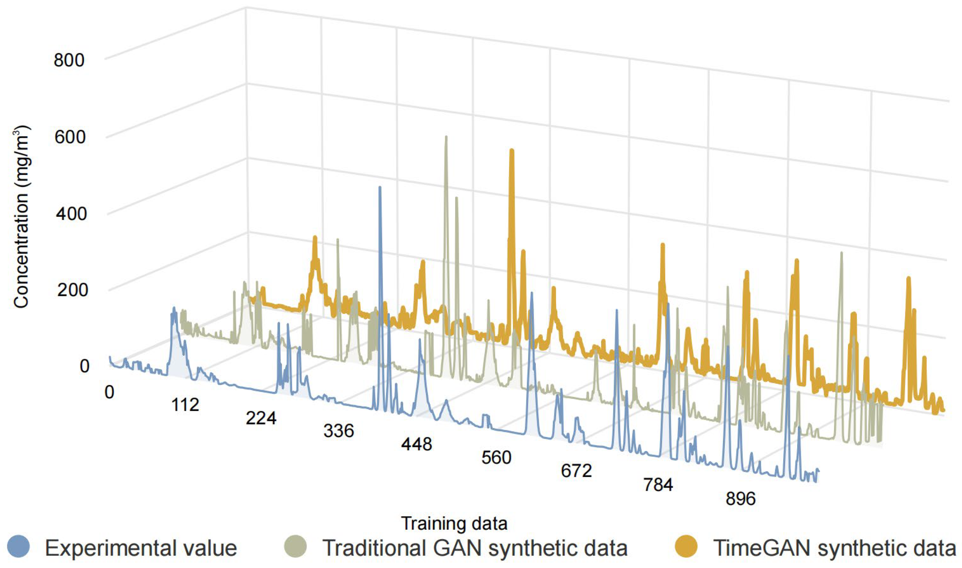
During the training process, the goal of TimeGAN is to generate time-series data that are statistically similar to the real data. First, the embedding network transforms the input time-series data into a low-dimensional representation that captures the intrinsic structure and patterns of the data. The recovery network then reverses this process, converting the low-dimensional representation back into the original time-series data, which helps the network learn the key features of the data. The generator then uses the mechanism of Generative Adversarial Networks to generate new time-series data to closely approximate the distribution of the real data. Finally, the discriminator discriminates between the generated time-series data and the real data, helping the generator to better simulate the distribution of the real data.

(3)

Feature extraction and fusion

This study used a combination of ResNet and a sparse attention mechanism to complete this crucial step. An attention branch parallel to ResNet was developed to improve the model’s ability to capture salient features. ResNet consists of several layers of one-dimensional networks, with the core structure consisting of convolutional, batch normalisation (BN), and pooling layers. The convolutional layers are responsible for local perception and feature extraction; the BN layers aim to accelerate the training process and improve model robustness; the pooling layers perform statistical operations on high-level features within the pooling region to output effective statistical features and achieve dimensionality reduction. The ResNet module contains two basic blocks, each consisting of successive convolutional layers, BN layers, and activation functions. The introduction of residual connections allows the network to learn complex feature representations more deeply. To further improve the model’s focus on important features and reduce the interference of unimportant features, a sparse attention module was introduced to address the limitations of ResNet in distinguishing the importance of temporal features. Following the literature [34,35], an element-wise multiplication method was used to fuse the outputs of the ResNet and attention mechanism modules, and these fused features are subsequently used as inputs to the TCN module.

(4)

Temporal Relationship Extraction

The model effectively captures the temporal dependencies between features through the TCN module and integrates them into the final prediction process. In this process, the input feature fusion results are first subjected to extended causal convolution operations, followed by processing through the ReLU activation function. To prevent model overfitting, a dropout layer is then introduced to randomly discard some nodes. The results of this process not only serve as input for further processing in the following diluted causal convolution, activation, and dropout layers but are also sent to a one-dimensional convolution layer for processing. The results of these two parts are linearly combined to form an output result with a residual connection, which is then sent to subsequent residual blocks for further computation. When the computation of all residual blocks is complete, the output of the residual blocks is combined with a fully connected layer and a softmax layer to produce the final prediction results.

(5)

Output of prediction results

In the previous processing, the data are normalised to eliminate the dimensional differences between different features. To obtain the final prediction results, the original scale of the predicted data is restored through a de-normalisation process, ensuring consistency with other relevant data and guaranteeing the interpretability and usability of the results. This step is an essential part of the entire prediction process and allows us to interpret and use the model output in a meaningful way. The calculation formula is shown in Equation (4).

$$x_o^L=x_{normal}^L\left(x_{\max }^L-x_{\min }^L\right)+x_{\min }^L$$

(4)

where $x_o^L$ is the predicted value after inverse normalisation; $x_{normal}^L$ is the predicted value output from the model; and $x_{\mathrm{m}\mathrm{a}\mathrm{x}}^L$ and $x_{\mathrm{m}\mathrm{i}\mathrm{n}}^L$ denote the maximum and minimum values of the original data, respectively.

The choice of model parameters is closely related to the type of task and dataset. Based on other similar studies, this study experimentally determined the appropriate parameters for the model [36,37,38,39,40,41]. The main parameter settings are presented in

Table 1. Main parameters.

Parameter	Mode and Value
Convolutional kernel	3 × 3
Pooling kernel	2 × 2
Residual block	2
Dilatation factor	2i (where i is the number of layers in the network)
Pooling strategy	Max pooling
Activation function	ReLU
Optimiser	Adam
Dropout	20%
Batch size	64
Epochs	30

.

3. Results and Discussion

3.1. Description of the Dataset

In the summer of 1956, the Prairie Grass Project was conducted, and the dataset it collected is still regarded as one of the most comprehensive in situ atmospheric dispersion datasets to date. It is capable of revealing patterns of hazardous gas diffusion. The experiment was conducted 5 miles northeast of O’Neill, Nebraska (42.49° N, 98.57° W). In the experiment, SO₂ was released from a point source at a height of 0.46 m above the ground. Air concentrations at a height of 1.5 m were sampled every 10 min at distances of 50, 100, 200, 400, and 800 m downwind. Given that the Prairie Grass Project’s dataset accurately reflects the diffusion of toxic gases in real-world environments, it was selected as the optimal data source for the simulation experiments conducted in this study [42,43,44,45]. The 68 sets of experimental data were divided into training and test sets, as shown in

Table 2. Division of training and test sets.

Dataset	Release Case	Number
Training set	Releases 1–60 (except for Releases 8, 16, 31, 35)	7068
Test set	Releases 61–68 and Releases 8, 16, 31, 35	1075

(where Release x is the number of the experiment). The common monitoring parameters in the Prairie Grass Project are shown in

Table 3. Monitoring parameters.

Parameters	Symbol	Unit
Downwind distance	Dx	m
Crosswind distance	Dy	m
Source strength	Q	g·s−1
Source height	Hs	m
Wind speed	V	m·s−1
Wind direction	Dir	deg
Atmospheric stability class	STA	/
Air temperature	T	°C
Heat flux	Fh	W·m−1
Mixing height	zm	m
Surface roughness height	Hs	m
Friction velocity in downwind direction	u*	m·s−1
Friction velocity in vertical direction	w*	m·s−1
Standard deviation of vertical velocity	σw	m·s−1
Standard deviation of direction	σd	m·s−1

.

3.2. Evaluation Indicators

To assess the model’s performance from multiple perspectives, this study employed the root mean square error (RMSE), mean absolute error (MAE), and the coefficient of determination (R²) as metrics, with Equations (5)–(7) providing the formulas. The MAE measures the total error, while the RMSE focuses on the impact of significant errors. Both are non-negative values, with lower values indicating better agreement between the predicted and actual results. R² represents the adequacy of the model fit to the data points, with a range from 0 to 1. A higher value indicates a better model fit.

$$RMSE=\sqrt{\frac{1}{N}\sum _{i=1}^N{\left(y_i^{exp}-y_i^{cal}\right)}^2}$$

(5)

$$MAE=\frac{1}{N}\sum _{i=1}^N\left|y_i^{exp}-y_i^{cal}\right|$$

(6)

$$R^2=1-\frac{{\sum }_{i=1}^N{\left(y_i^{exp}-y_i^{cal}\right)}^2}{{\sum }_{i=1}^N{\left(y_{ave}^{exp}-y_i^{exp}\right)}^2}$$

(7)

where N represents the total number of data points, and $y_i^{exp}$, $y_i^{cal}$, and $y_{ave}^{exp}$ correspond to the experimental, calculated, and average values of the experiments, respectively.

3.3. Experimental Result Analysis

3.3.1. Validation of Model Prediction Results

To qualitatively assess the accuracy of TimeGAN-synthesised data, this study adopted a comparative approach based on real data trends. Specifically, the similarity between real data, TimeGAN-synthesised data, and traditional GAN-synthesised data is determined using 1000 randomly selected training datasets as benchmarks. This comparison shows the effectiveness of the synthetic data in simulating the real data distribution, thus validating the performance of the TimeGAN model in the data generation task. The experimental results are shown in Figure 5.

As can be seen in Figure 5, compared to the data synthesised by the traditional GAN, the dataset synthesised by TimeGAN showed a greater ability to simulate real data trends. While the traditional GAN typically works to capture the distributional characteristics of data, when dealing with time-dependent sequential data, this approach tends to ignore the dynamic correlations and temporal dependencies in the time series. TimeGAN was designed with this unique property of temporal data in mind. It learns and preserves the evolutionary patterns of data over time through embedded temporal correlation structures, producing synthetic data that not only resembles the original data in terms of static distribution but also more accurately reflects the characteristics of the original time-series data in terms of dynamic trends. This makes TimeGAN a more desirable choice for data analysis and predictive models that need to account for temporal dynamics.

To ensure the effectiveness of model training and to assess the quality of the data generated by TimeGAN, a 5-fold cross-validation method was used in this study. K-fold cross-validation is commonly used to evaluate the performance of deep learning models, especially when dealing with time-series data, where it is crucial to avoid random breaks in the data. This ensures that the continuity and integrity of the time-series data are maintained, allowing the model to effectively capture the dynamics of the time series. Using this approach, we compared the performance of models trained on raw data, TimeGAN-synthesised data, and GAN-synthesised data under the same conditions to confirm the validity and reliability of the synthetic data. The experimental results are presented in

Table 4. Cross-validation to assess the quality of synthetic data.

Methods	RMSE	MAE	R2
Real data	19.2977	9.9089	0.8593
TimeGAN-synthesised data	13.6521	6.6283	0.9697
GAN-synthesised data	16.6654	8.0092	0.7991

.

When evaluating the performance differences between the models trained on data synthesised by TimeGAN and those trained on original data, the research indicated that the data synthesised by TimeGAN demonstrate superior performance on three key metrics: the RMSE, MAE, and R². Specifically, the models trained on TimeGAN-synthesised data showed a reduction in the RMSE from 19.12977 to 13.6521, the MAE from 9.9089 to 6.6283, and an improvement in R² from 0.8593 to 0.9697. This result demonstrates that TimeGAN-synthesised data perform exceptionally well in simulating the statistical characteristics and time dependencies of real datasets, allowing models to more accurately capture data patterns and, thus, improve the accuracy of predictive tasks. A further comparison between the models trained on TimeGAN-synthesised data and those trained on traditional GAN-synthesised data showed significant differences. The models trained on TimeGAN-synthesised data outperformed those trained on traditional GAN-synthesised data in terms of the RMSE, MAE, and R², with the former having lower RMSE and MAE values and an R² value closer to the ideal of 1. This difference in performance may be due to the specialised design of TimeGAN for time-series data, as it better captures the overall distribution and temporal correlations. In contrast, the traditional GAN may not fully capture the dynamic nature of time-series data, thereby affecting the final predictive performance. In conclusion, using TimeGAN for data augmentation provides a high-quality database for model training, which significantly improves the predictive power of the model.

Since the model complexity comes from the network structure, we used dropout regularisation to globally control the model complexity during model training in order to reduce the possibility of overfitting. The experimental results are shown in

Table 5. Improved model performance through regularisation.

Method	Dataset	RMSE	MAE	R2
Regularisation applied	Training set	11.5601	5.9901	0.9812
	Test set	13.6521	6.6283	0.9697
No regularisation applied	Training set	15.2231	7.5721	0.8321
	Test set	16.6654	8.0092	0.7985

.

In this study, the predictions of the model were validated by comparing them with real-world data to ensure the accuracy and usefulness of the predictions. Figure 6 shows the relationship between the predicted outputs of the model and real-world data. Through a comparison and validation with real-world data, we found that there was a high degree of consistency between the model’s predicted output and the actual data. This not only indicates that the proposed model has a good predictive capability but also confirms that the model does not suffer from bias in the predicted output. In other words, the model can accurately capture the intrinsic trends of data and maintain a high degree of accuracy in its predictions.

3.3.2. Ablation Experiments

Ablation experiments are employed to investigate how the specific components of a model impact its performance by systematically removing them. This experimental approach provides readers with insights into the role that each component plays in the model’s overall performance and helps validate the model’s design rationale.

In the ablation experiments, the proposed model served as a baseline, and we evaluated the performance gap between the model and the baseline model by excluding the components TimeGAN, SA, TCN, and ResNet, one by one. Figure 7 and

Table 6. Results of the ablation experiment (w/o means without).

Ablation Experiment	Methods	RMSE	MAE	R2
Abl exp. 1 (baseline)	SAResNet-TCN	13.6521	6.6283	0.9697
Abl exp. 2	(w/o) TimeGAN	19.9331	9.9841	0.8501
Abl exp. 3	(w/o) SA mechanism	21.0213	10.0214	0.8201
Abl exp. 4	(w/o) TCN	26.7234	17.6549	0.8312
Abl exp. 5	(w/o) ResNet	29.7069	20.8541	0.7601

show the results of the ablation experiment. Compared to ablation experiment 2 (Abl exp. 2), it is clear that the model without data augmentation did not perform well on the test set containing unseen data and, thus, it lacks a generalisation ability. As demonstrated by the results of Abl exp. 3, the model’s RMSE increased by over 25% upon the removal of the SA mechanism module. Figure 7b,c shows that removing the SA mechanism module significantly reduced the model’s ability to predict peaks and troughs. This suggests that the SA mechanism helps the model to focus on crucial information within the sequence, thereby improving its accuracy in predicting abrupt changes. According to the results of Abl exp. 4 and Abl exp. 5, the TCN and ResNet modules have a significant impact on the performance of the overall model. ResNet has translational invariance, and TCN has temporal invariance. Combining the advantages of both can strengthen the model’s ability to perceive spatial and temporal relationships.

3.3.3. Comparison Experiment

The performance of the proposed model was evaluated by comparing it with that of other models with different configurations. The comparison experiments revealed the limitations and room for improvement in the model design and helped in selecting the most appropriate model to achieve the desired results.

Figure 8 illustrates the prediction results of the model incorporating different attention mechanisms. It was observed that the model without an attention mechanism had the poorest performance. Compared to the use of multi-head attention (Mh_A) mechanisms, the SA mechanism demonstrated a remarkable improvement in the model’s prediction results. The SA mechanism excels at homing in on important task-relevant information and precisely allocating attentional weights. This not only strengthens the model’s performance and ability to generalise but also reduces the likelihood of overfitting. Although the attention mechanism may lengthen the model’s training time, its significant advantages render it an efficient tool for enhancing prediction accuracy. The SA mechanism has the potential to decrease computational time while also expressing attention when compared to the use of Mh_A mechanisms in model prediction. The reduction in computation time provided by the SA mechanism not only increases its potential applicability in various scenarios but is also particularly important in the case of sudden toxic gas leaks. This advancement means that the relevant authorities can respond and carry out rescue operations more quickly, effectively reducing the impact of pollution incidents on human health and public safety.

In the comparison experiment, we applied different models and combined them to determine the optimal model combination. The outcomes of the error comparison between the predictions of the proposed model and those of the SACNN-TCN, SABPNN-TCN, SAResNet-LSTM, and SAResNet-GRU models are shown in Figure 9. The results demonstrated a poor performance of the fusion model using a backpropagation neural network (BPNN), with an absolute error of more than 80 mg/m³ in the peak value. This could be attributed to BPNN being based on gradient optimisation, which is susceptible to locally optimal solutions, and it is challenging for it to access the global optimal solution. In contrast to SACNN-TCN, the proposed model exhibited advantageous performance in forecasting. The peak absolute error of SACNN-TCN exceeded 60 mg/m³, whereas the proposed model’s peak absolute error was less than 40 mg/m³. In addition, the proposed model demonstrated greater predictive stability, exhibiting less overall deviation from the true value. This advantage is attributable to the inclusion of residual concatenation, which enables ResNet to learn incremental changes in features, thereby capturing information in the input data more efficiently. It is evident that SAResNet-GRU, using long short-term memory (LSTM) and the gated recurrent unit (GRU), which are variations of the Recurrent Neural Network (RNN) used for forecasting, outperformed SAResNet-LSTM. This phenomenon can be ascribed to the reset gate mechanism within the GRU, which enhances the model’s flexibility. This adaptability enables the GRU to better adapt to patterns in sequences with different time scales, leading to improved performance in predictive tasks. However, compared to the GRU, the TCN achieved more efficient gradient propagation through convolutional operations. Therefore, the proposed model exhibited better stability and exceptional predictive capabilities.

3.4. Interpretation and Application

3.4.1. GSA

Deep learning models are effective in various tasks but often lack interpretability, which causes several problems [46]. Firstly, environmental managers and decision-makers may struggle to understand the model’s reasoning, reducing their trust. Secondly, unclear predictions could lead to misinterpretations, particularly for critical tasks involving life and environment preservation, resulting in serious consequences.

GSA is critical when determining the impact of input parameters on a model’s output, allowing researchers to identify parameters that require more precise measurement or careful adjustments. The Sobol method is a GSA approach that quantifies the contribution of each parameter to the variance in the total model output, either through changes in the parameter itself or through interactions with other parameters [46,47,48]. The results of the Sobol method analysis are depicted in Figure 10. Wind speed, atmospheric stability class, and source strength (the mass of pollutant emitted from a source into the atmosphere per unit of time) were the most significant factors influencing the dispersion of pollutants. The last seven indicators, such as the directional standard deviation, were of relatively minor importance. For a better comprehension of how the input indicators impact the predictive performance of the model, an additive-by-addition approach was employed. This involved progressively adding the indicators based on their contribution in order to gauge their impact on the model’s predictive capacity. The experimental results shown in Figure 11 clearly demonstrate that removing metrics with minimal contributions to model performance had a negligible impact on the accuracy of its predictions. Consequently, when resource limitations preclude access to all parameters, researchers should prioritise those that exert a pronounced influence on model output. In such resource-constrained scenarios, a high prediction accuracy can still be achieved by selecting key input parameters such as downwind distance, crosswind distance, source strength, source height, wind speed, wind direction, atmospheric stability class, and air temperature. These parameters are ideal for high-precision forecasting because they play a crucial role in simulating the dispersion of pollutants in the atmosphere. The results presented in Figure 8 demonstrate that focusing on the parameters that contribute most significantly to predictive accuracy is an effective strategy for maintaining the predictive performance of a model when not all parameters are available.

3.4.2. Application of Hazard Threshold Analysis

To further enhance the usefulness of this study, the maximum downwind hazardous distance (MDH-distance) based on different SO₂ hazard thresholds was visualised. In particular, we used Release 31 as a case study and calculated the release concentrations according to the six weather conditions specified in GBT37243-2019 [21]. Figure 12 depicts the change in the MDH-distance over different hazard thresholds. An explanation of these hazard thresholds is given in

Table 7. Hazard thresholds for toxic gas SO₂ injuries.

Hazard Class	Definition	Concentration
PAC—1	Minor and temporary health effects	0.2 ppm
PAC—2	Serious irreversible health effects	0.75 ppm
PAC—3	Endangering life or causing death	30 ppm
IDLH	Occupational exposure limit values	100 ppm

. The Protective Action Criteria (PAC) were established by the Subcommittee on Consequence Assessment and Protective Actions (SCAPA). SCAPA is a subcommittee of the United States Department of Energy (DOE). The PAC serve as a tool for assessing the severity of the consequences of uncontrolled toxic releases. They help to assess the impact of such releases and guide the planning of appropriate responses. Immediately Dangerous to Life or Health (IDLH) limits deal specifically with high concentrations of hazardous substances that can endanger human life. This standard focuses primarily on the protection of workers in industrial environments and provides a basis for assessing and selecting appropriate protective equipment for use in the workplace.

According to Figure 12, a distinct gap is evident in the MDH-distance for different conditions. Specifically, the MDH-distance reached its maximum value under conditions of atmospheric stability class F and a wind speed of 1.5 m/s. The MDH-distance achieved its lowest value under atmospheric stability class D conditions and a wind speed of 8.5 m/s. More specifically, at the PAC-1 level, the MDH-distance ranged from 822 to 1354 m, with a remarkable variance of 64.72%. As for the level of PAC-2, the MDH-distance range laid between 555 and 1204 m, with a relative difference as high as 116.94%. There was also a major difference between the MDH-distance ranges of PAC-3 and IDLH. According to the above findings, the MDH-distance is greater at low wind speeds and high atmospheric stability. The reason for this phenomenon lies in the fact that, when wind speeds are low and atmospheric stability is high, air movement is limited. This makes it challenging for pollutants to diffuse and dilute quickly. Consequently, the spread of contaminants on the downwind decelerates, increasing the likelihood of accumulation and consequently expanding the MDH-distance. Under similar wind speeds, increased atmospheric stability reduces updrafts, resulting in a slower vertical blending of pollutants. As a result, the dilution capacity of the pollutants is decreased, leading to an increase in the MDH-distance. This discovery highlights the impact of wind speed and atmospheric stability on pollutant dispersal and establishes a crucial scientific foundation for environmental regulation. It is vital to emphasise that exceeding the PAC-2 threshold endangers individuals’ health and weakens their capacity for self-protection. Therefore, authorities need to issue real-time warnings based on the wind speed and atmospheric stability class and evacuate people in time to prevent severe safety incidents. In addition, ensuring a high level of safety is particularly important when undertaking rescue activities or emergency responses. Beyond the IDLH threshold, only highly reliable respiratory equipment is permitted to ensure that personnel are adequately protected in the performance of their duties. These safety measures are not only effective at reducing the risk of exposure to rescuers but also in ensuring the safety of the public.

3.5. Discussion

Deep learning models have demonstrated considerable potential in forecasting the dispersion of hazardous gases due to their capacity to adapt autonomously based on training data, thereby generating more reliable forecasts. However, the efficacy of these models is contingent upon the representativeness of the training data. In particular, when models are constructed using data from specific geographic regions, their applicability may be constrained in other areas with disparate terrains, seasons, or soil types. The dataset utilised in this study originated from a point-source continuous emission experiment, which was of limited duration and did not encompass seasonal variations or changes in geographic location. Consequently, the research investigated the impact of short-term environmental factors, such as wind speed, on the diffusion of hazardous gases. While factors such as seasonal changes and geographic location also affect the dispersion of hazardous gases, these variables were not extensively discussed in this study, given that the aim was to develop innovative deep learning models and validate their performance using data from the Prairie Grass Project. Overall, deep learning models demonstrate great potential in predicting the dispersion of hazardous gases. However, to advance deep learning models in the field of environmental sustainability, it is essential to explore and enhance their applicability and accuracy in diverse environments.

4. Conclusions

This paper presented exploratory research aimed at addressing the problem of predicting pollutant dispersion using deep learning techniques. The main contributions are outlined below.

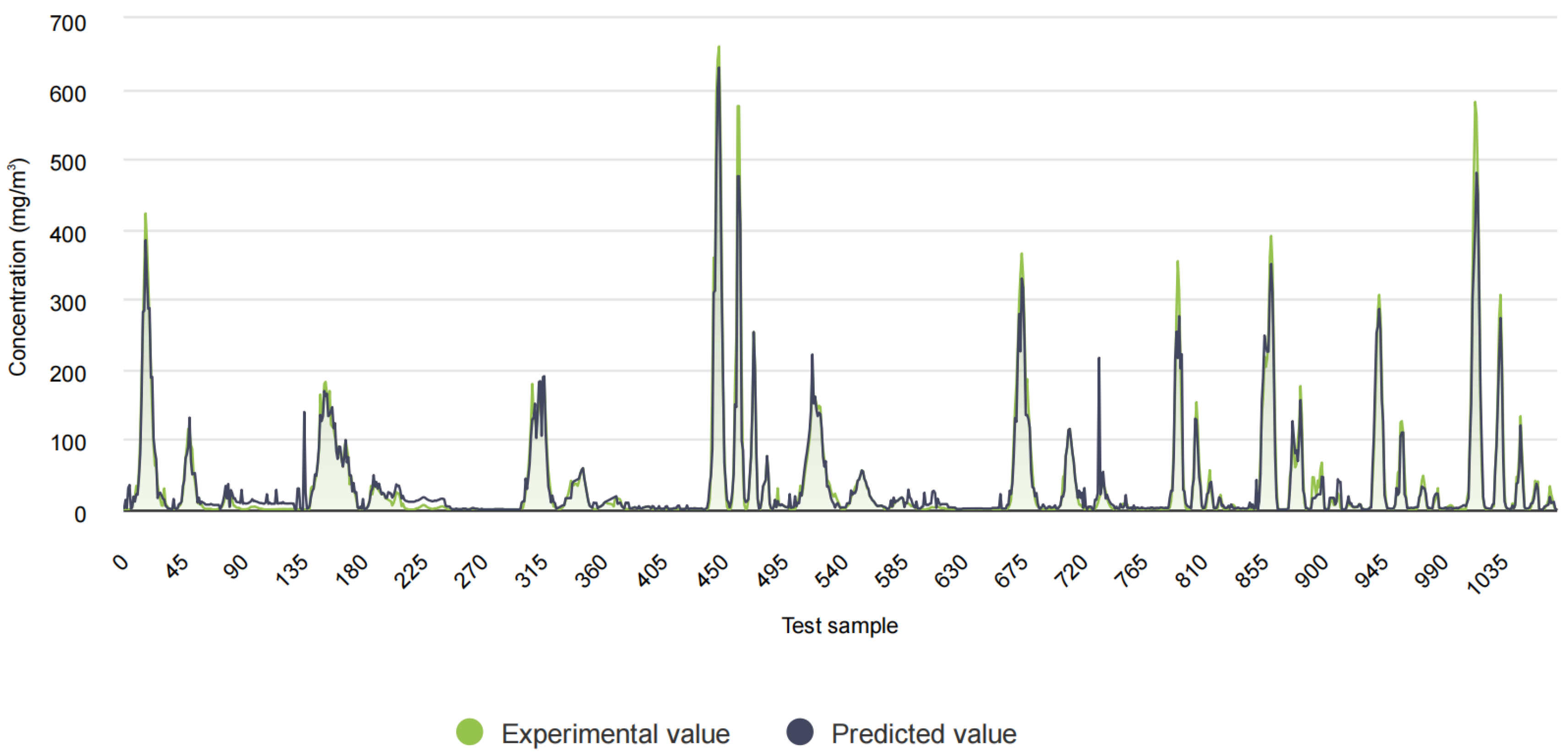
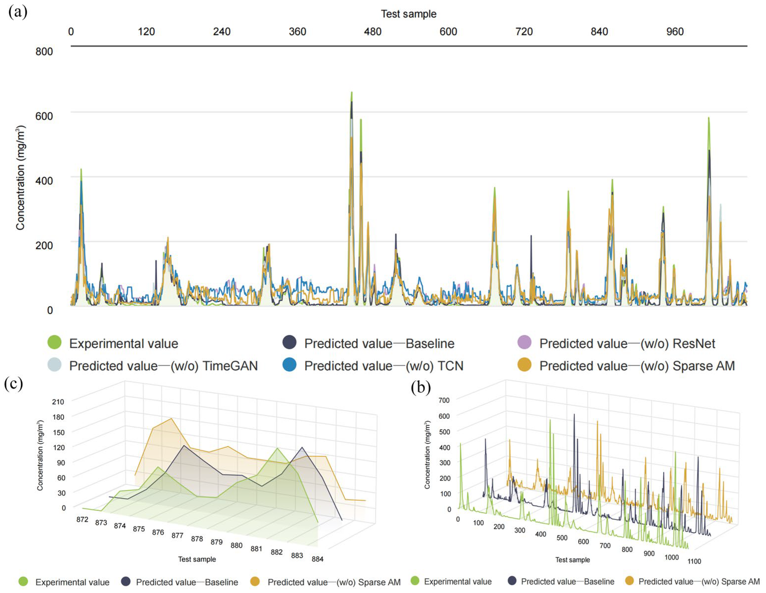
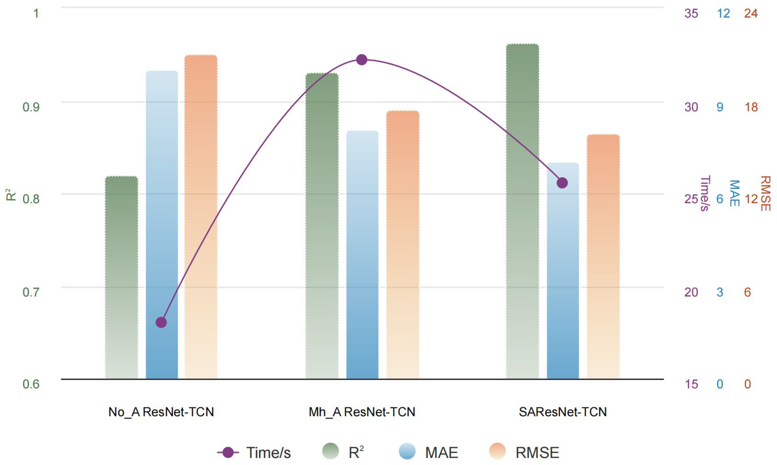
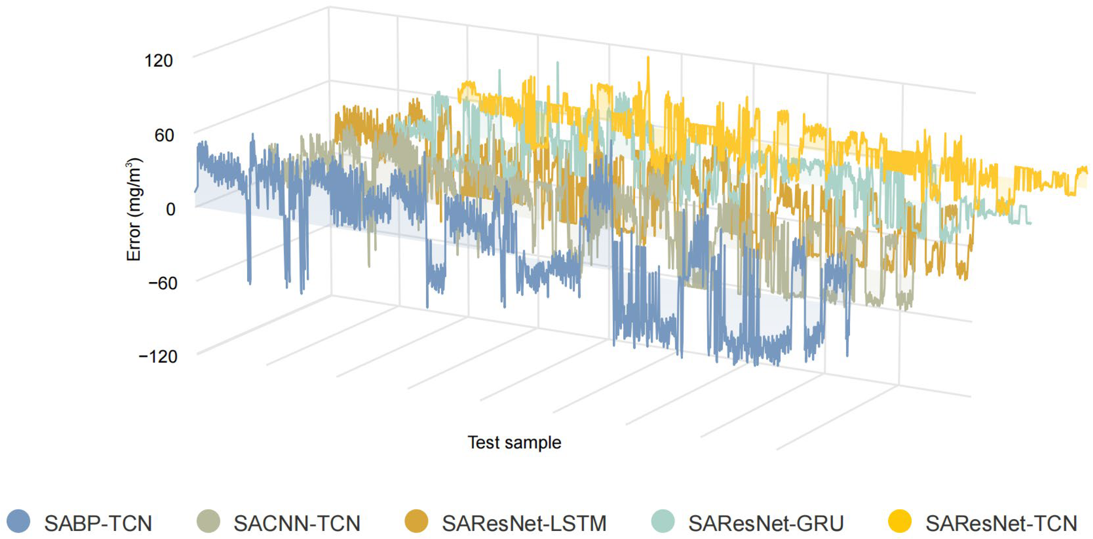
1. The proposed model exhibited remarkable predictive efficacy. Ablation experiments were conducted to further substantiate the significant impact of key components, including TimeGAN, SA, TCN, and ResNet, on the overall model performance. Notably, the removal of the SA mechanism led to an increase of over 25% in the model’s RMSE value, which serves to underscore the critical importance of the SA mechanism in enhancing the model’s performance. Furthermore, the results of the comparative experiments demonstrated a clear advantage of the proposed model over other models with different configurations. This was confirmed by the superior performance of the proposed model in terms of the RMSE, MAE, and R² values, which were 3.6521, 6.6283, and 0.9697, respectively.

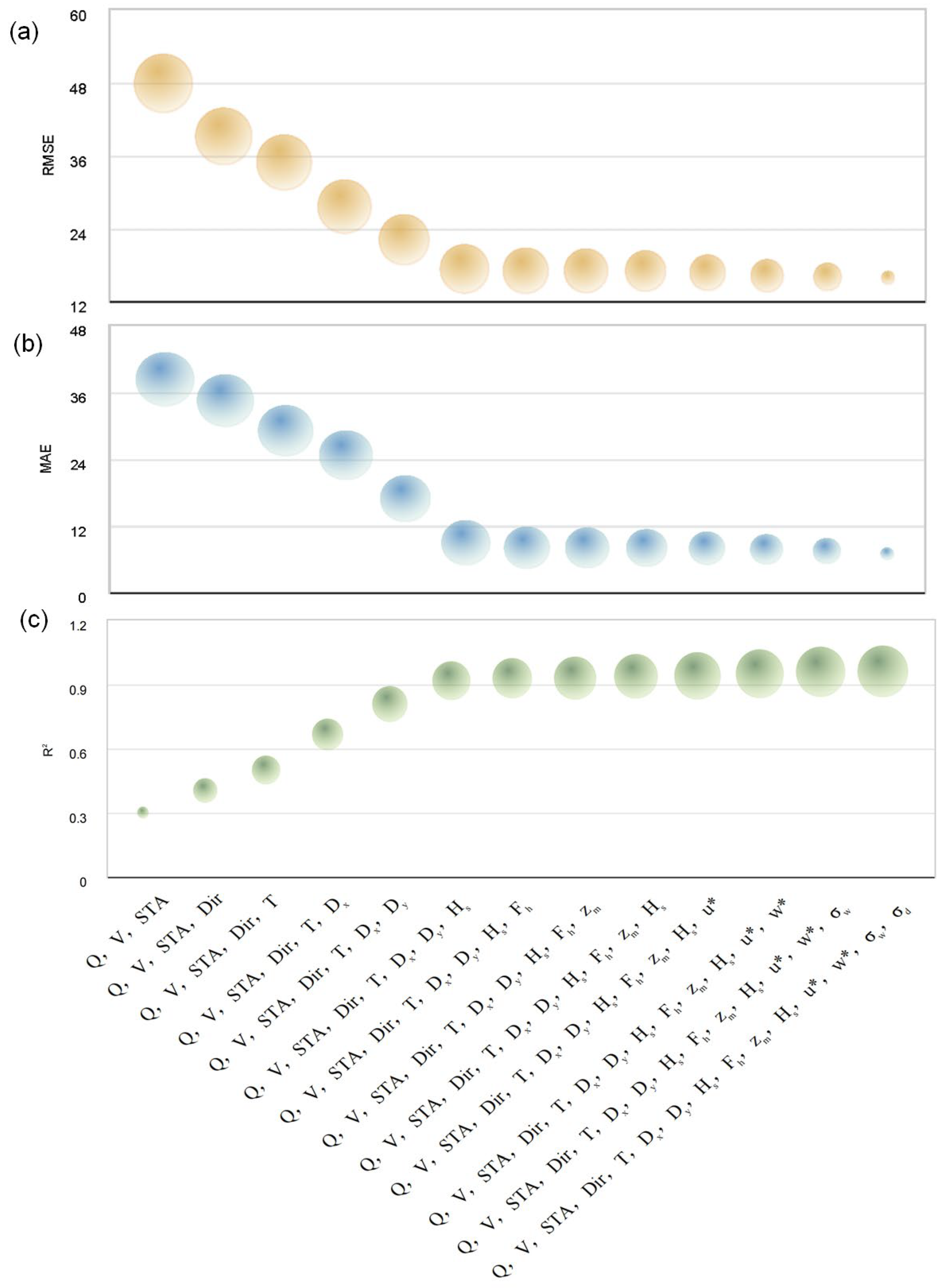
2. This study used GSA to improve the interpretability of the results. The results of the additive-by-addition method identified less significant indicators and the optimal combination of inputs for different scenarios. This provides a practical solution for forecasting tasks, particularly in situations where resources are limited and it is difficult to obtain all the parameters.

3. This study calculated the MDH-distance for different wind speeds and atmospheric stability conditions, using PAC and IDLH values as hazard thresholds. Such an analysis will assist relevant authorities in accurately predicting and assessing the impact of air pollution incidents, thereby improving the effectiveness and credibility of emergency responses.

References

1. Torchio, M.F.; Lucia, U.; Grisolia, G. Development Indexes, Environmental Cost Impact, and Well-Being: Trends and Comparisons in Italy. Sustainability 2024, 16, 4380. [Google Scholar] [CrossRef]
2. Hu, Y.; Chao, K.; Zhu, Z.; Yue, J.; Qie, X.; Wang, M. A Study on a Health Impact Assessment and Healthcare Cost Calculation of Beijing–Tianjin–Hebei Residents under PM2.5 and O3 Pollution. Sustainability 2024, 16, 4030. [Google Scholar] [CrossRef]
3. Yuval; Levi, Y.; Broday, D.M. Revealing Causality in the Associations between Meteorological Variables and Air Pollutant Concentrations. Environ. Pollut. 2024, 345, 123526. [Google Scholar] [CrossRef]
4. Yang, J.; Shi, L.; Lee, J.; Ryu, I. Spatiotemporal Prediction of Particulate Matter Concentration Based on Traffic and Meteorological Data. Transp. Res. Part D Transp. Environ. 2024, 127, 104070. [Google Scholar] [CrossRef]
5. Ma, Z.; Wang, B.; Luo, W.; Jiang, J.; Liu, D.; Wei, H.; Luo, H. Air Pollutant Prediction Model Based on Transfer Learning Two-Stage Attention Mechanism. Sci. Rep. 2024, 14, 7385. [Google Scholar] [CrossRef]
6. Zhang, Z.; Johansson, C.; Engardt, M.; Stafoggia, M.; Ma, X. Improving 3-Day Deterministic Air Pollution Forecasts Using Machine Learning Algorithms. Atmos. Chem. Phys. 2024, 24, 807–851. [Google Scholar] [CrossRef]
7. Amiri, A.F.; Kichou, S.; Oudira, H.; Chouder, A.; Silvestre, S. Fault Detection and Diagnosis of a Photovoltaic System Based on Deep Learning Using the Combination of a Convolutional Neural Network (CNN) and Bidirectional Gated Recurrent Unit (Bi-GRU). Sustainability 2024, 16, 1012. [Google Scholar] [CrossRef]
8. Yang, X.; Zhou, J.; Zhang, Q.; Xu, Z.; Zhang, J. Evaluation and Interpretation of Runoff Forecasting Models Based on Hybrid Deep Neural Networks. Water Resour. Manag. 2024, 38, 1987–2013. [Google Scholar] [CrossRef]
9. Zeng, W.; Lin, Q.; Zhu, B.; Peng, C.; Yu, R. Modeling Vehicle U-Turning Behavior near Intersections: A Deep Learning Approach Based on TCN and Multi-Head Attention. Expert Syst. Appl. 2024, 249, 123674. [Google Scholar] [CrossRef]
10. Wang, S.; McGibbon, J.; Zhang, Y. Predicting High-Resolution Air Quality Using Machine Learning: Integration of Large Eddy Simulation and Urban Morphology Data. Environ. Pollut. 2024, 344, 123371. [Google Scholar] [CrossRef]
11. Xu, H.; Tian, Y.; Ren, H.; Liu, X. A Lightweight Channel and Time Attention Enhanced 1D CNN Model for Environmental Sound Classification. Expert Syst. Appl. 2024, 249, 123768. [Google Scholar] [CrossRef]
12. Gao, J.; Guo, J.; Yuan, F.; Yi, T.; Zhang, F.; Shi, Y.; Li, Z.; Ke, Y.; Meng, Y. An Exploration into the Fault Diagnosis of Analog Circuits Using Enhanced Golden Eagle Optimized 1D-Convolutional Neural Network (CNN) with a Time-Frequency Domain Input and Attention Mechanism. Sensors 2024, 24, 390. [Google Scholar] [CrossRef] [PubMed]
13. Wang, M.; Ye, X.-W.; Jia, J.-D.; Ying, X.-H.; Ding, Y.; Zhang, D.; Sun, F. Confining Pressure Forecasting of Shield Tunnel Lining Based on GRU Model and RNN Model. Sensors 2024, 24, 866. [Google Scholar] [CrossRef] [PubMed]
14. Zheng, K.; Wang, J.; Chen, Y.; Jiang, R.; Wang, W. DDTCN: Decomposed Dimension Time-Domain Convolutional Neural Network along Spatial Dimensions for Multiple Long-Term Series Forecasting. Appl. Intell. 2024. [Google Scholar] [CrossRef]
15. Ma, Z.; Sun, Y.; Ji, H.; Li, S.; Nie, S.; Yin, F. A CNN-BiLSTM-Attention Approach for EHA Degradation Prediction Based on Time-Series Generative Adversarial Network. Mech. Syst. Signal Process. 2024, 215, 111443. [Google Scholar] [CrossRef]
16. Du, A.; Zhou, Q.; Dai, Y. Methodology for Evaluating the Generalization of ResNet. Appl. Sci. 2024, 14, 3951. [Google Scholar] [CrossRef]
17. Hassan, S.M.; Maji, A.K. Pest Identification Based on Fusion of Self-Attention With ResNet. IEEE Access 2024, 12, 6036–6050. [Google Scholar] [CrossRef]
18. Cheng, L.; Liu, Z.; Ma, Q.; Qi, H.; Qi, F.; Zhang, Y. An Attention-Based Full-Scale Fusion Network for Segmenting Roof Mask from Satellite Images. Appl. Sci. 2024, 14, 4371. [Google Scholar] [CrossRef]
19. Al-Gaashani, M.S.A.M.; Muthanna, A.; Chelloug, S.A.; Kumar, N. EAMultiRes-DSPP: An Efficient Attention-Based Multi-Residual Network with Dilated Spatial Pyramid Pooling for Identifying Plant Disease. Neural Comput. Appl. 2024. [Google Scholar] [CrossRef]
20. Yu, Y.; Zhang, Y.; Cheng, Z.; Song, Z.; Tang, C. Multi-Scale Spatial Pyramid Attention Mechanism for Image Recognition: An Effective Approach. Eng. Appl. Artif. Intell. 2024, 133, 108261. [Google Scholar] [CrossRef]
21. GBT37243-2019; Determination Method of External Safety Distance for Hazardous Chemicals Production Units and Storage Installations. Ministry of Emergency Management: Beijing, China, 2019.
22. He, F.; Liu, T.; Tao, D. Why ResNet Works? Residuals Generalize. IEEE Trans. Neural Netw. Learn. Syst. 2020, 31, 5349–5362. [Google Scholar] [CrossRef]
23. Bai, S.; Kolter, J.Z.; Koltun, V. An Empirical Evaluation of Generic Convolutional and Recurrent Networks for Sequence Modeling. arXiv 2018, arXiv:1803.01271. [Google Scholar]
24. Mezina, A.; Burget, R.; Travieso-González, C.M. Network Anomaly Detection With Temporal Convolutional Network and U-Net Model. IEEE Access 2021, 9, 143608–143622. [Google Scholar] [CrossRef]
25. Samal, K.K.R.; Babu, K.S.; Das, S.K. Temporal Convolutional Denoising Autoencoder Network for Air Pollution Prediction with Missing Values. Urban Clim. 2021, 38, 100872. [Google Scholar] [CrossRef]
26. Vaswani, A.; Shazeer, N.; Parmar, N.; Uszkoreit, J.; Jones, L.; Gomez, A.N.; Kaiser, L.; Polosukhin, I. Attention Is All You Need. In Proceedings of the Advances in Neural Information Processing Systems 30 (NIPS 2017), Long Beach, CA, USA, 4–9 December 2017. [Google Scholar]
27. Pan, X.; Ge, C.; Lu, R.; Song, S.; Chen, G.; Huang, Z.; Huang, G. On the Integration of Self-Attention and Convolution. In Proceedings of the Advances in Neural Information Processing Systems 35 (NIPS 2022), New Orleans, LA, USA, 28 November–9 December 2022. [Google Scholar]
28. Mnih, V.; Heess, N.; Graves, A.; Kavukcuoglu, K. Recurrent Models of Visual Attention. In Proceedings of the Advances in Neural Information Processing Systems 27 (NIPS 2014), Montreal, QC, Canada, 8–13 December 2014. [Google Scholar]
29. Zhou, H.; Zhang, S.; Peng, J.; Zhang, S.; Li, J.; Xiong, H.; Zhang, W. Informer: Beyond Efficient Transformer for Long Sequence Time-Series Forecasting. In Proceedings of the AAAI Conference on Artificial Intelligence, Virtually, 2–9 February 2021; Volume 35, pp. 11106–11115. [Google Scholar]
30. Yu, M.; Masrur, A.; Blaszczak-Boxe, C. Predicting Hourly PM2.5 Concentrations in Wildfire-Prone Areas Using a SpatioTemporal Transformer Model. Sci. Total Environ. 2023, 860, 160446. [Google Scholar] [CrossRef]
31. Neubürger, F.; Saeid, Y.; Kopinski, T. TimeGAN for Data-Driven AI in High-Dimensional Industrial Data. In Proceedings of the International Conference on Advances in Data-Driven Computing and Intelligent Systems, Pilani, India, 21–23 September 2023; Springer: Singapore, 2024; pp. 473–484. [Google Scholar]
32. Liang, G.; Hu, J.; Yang, K.; Song, S.; Liu, T.; Xie, N.; Yu, Y. Data Augmentation for Predictive Digital Twin Channel: Learning Multi-Domain Correlations by Convolutional TimeGAN. IEEE J. Sel. Top. Signal Process. 2024, 18, 18–33. [Google Scholar] [CrossRef]
33. Tai, C.-Y.; Wang, W.-J.; Huang, Y.-M. Using Time-Series Generative Adversarial Networks to Synthesize Sensing Data for Pest Incidence Forecasting on Sustainable Agriculture. Sustainability 2023, 15, 7834. [Google Scholar] [CrossRef]
34. Wang, P.; Li, W.; Gao, Z.; Zhang, Y.; Tang, C.; Ogunbona, P. Scene Flow to Action Map: A New Representation for RGB-D Based Action Recognition with Convolutional Neural Networks. In Proceedings of the 2017 IEEE Conference on Computer Vision and Pattern Recognition (CVPR), Honolulu, HI, USA, 26 July 2017; pp. 416–425. [Google Scholar]
35. Hyndman, R.J.; Koehler, A.B. Another Look at Measures of Forecast Accuracy. Int. J. Forecast. 2006, 22, 679–688. [Google Scholar] [CrossRef]
36. Springenberg, J.T.; Dosovitskiy, A.; Brox, T.; Riedmiller, M. Striving for Simplicity: The All Convolutional Net. arXiv 2015, arXiv:1412.6806. [Google Scholar]
37. Tao, Q.; Liu, F.; Li, Y.; Sidorov, D. Air Pollution Forecasting Using a Deep Learning Model Based on 1D Convnets and Bidirectional GRU. IEEE Access 2019, 7, 76690–76698. [Google Scholar] [CrossRef]
38. Nieto-Hidalgo, M.; Gallego, A.-J.; Gil, P.; Pertusa, A. Two-Stage Convolutional Neural Network for Ship and Spill Detection Using SLAR Images. IEEE Trans. Geosci. Remote Sens. 2018, 56, 5217–5230. [Google Scholar] [CrossRef]
39. Nhu, V.-H.; Hoang, N.-D.; Nguyen, H.; Ngo, P.T.T.; Thanh Bui, T.; Hoa, P.V.; Samui, P.; Tien Bui, D. Effectiveness Assessment of Keras Based Deep Learning with Different Robust Optimization Algorithms for Shallow Landslide Susceptibility Mapping at Tropical Area. Catena 2020, 188, 104458. [Google Scholar] [CrossRef]
40. Kingma, D.; Ba, J. Adam: A Method for Stochastic Optimization. In Proceedings of the 3rd International Conference for Learning Representations (Iclr’15), San Diego, CA, USA, 7–9 May 2015; Volume 500. [Google Scholar]
41. Cheng, G.; Han, J.; Zhou, P.; Xu, D. Learning Rotation-Invariant and Fisher Discriminative Convolutional Neural Networks for Object Detection. IEEE Trans. Image Process. 2018, 28, 265–278. [Google Scholar] [CrossRef] [PubMed]
42. Ma, D.; Zhang, Z. Attention Is All You Need. J. Hazard. Mater. 2016, 311, 237–245. [Google Scholar] [CrossRef] [PubMed]
43. Wang, Y.; Chen, B.; Zhu, Z.; Wang, R.; Chen, F.; Zhao, Y.; Zhang, L. A Hybrid Strategy on Combining Different Optimization Algorithms for Hazardous Gas Source Term Estimation in Field Cases. Process Saf. Environ. Prot. 2020, 138, 27–38. [Google Scholar] [CrossRef]
44. Shi, T.; Han, Z.; Gong, W.; Ma, X.; Han, G. High-Precision Methodology for Quantifying Gas Point Source Emission. J. Clean. Prod. 2021, 320, 128672. [Google Scholar] [CrossRef]
45. Qian, F.; Chen, L.; Li, J.; Ding, C.; Chen, X.; Wang, J. Direct Prediction of the Toxic Gas Diffusion Rule in a Real Environment Based on LSTM. Int. J. Environ. Res. Public Health 2019, 16, 2133. [Google Scholar] [CrossRef] [PubMed]
46. Jiang, Y.; Li, C.; Zhang, Y.; Zhao, R.; Yan, K.; Wang, W. Data-Driven Method Based on Deep Learning Algorithm for Detecting Fat, Oil, and Grease (FOG) of Sewer Networks in Urban Commercial Areas. Water Res. 2021, 207, 117797. [Google Scholar] [CrossRef] [PubMed]
47. Khorashadi Zadeh, F.; Nossent, J.; Sarrazin, F.; Pianosi, F.; van Griensven, A.; Wagener, T.; Bauwens, W. Comparison of Variance-Based and Moment-Independent Global Sensitivity Analysis Approaches by Application to the SWAT Model. Environ. Model. Softw. 2017, 91, 210–222. [Google Scholar] [CrossRef]
48. Mukherjee, I.; Singh, U.K. Characterization of Groundwater Nitrate Exposure Using Monte Carlo and Sobol Sensitivity Approaches in the Diverse Aquifer Systems of an Agricultural Semiarid Region of Lower Ganga Basin, India. Sci. Total Environ. 2021, 787, 147657. [Google Scholar] [CrossRef]
Figure 1. Diagram of basic modules of ResNet.
Sustainability 16 04531 g001
Figure 2. Diagram of basic modules of a TCN: (a) dilated causal convolution layer, (b) residual block.
Sustainability 16 04531 g002
Figure 3. Schematic illustrating how TimeGAN generates data.
Sustainability 16 04531 g003
Figure 4. The main structure of the proposed model.
Sustainability 16 04531 g004
Figure 5. Validation of synthetic data quality with real data.
Sustainability 16 04531 g005
Figure 6. Validation of predictions with real-world data.
Sustainability 16 04531 g006
Figure 7. Results of ablation experiments: (a) all ablation experiments; (b) results of Abl exp. 3; (c) comparison of peak predictions for Abl exp. 3.
Sustainability 16 04531 g007
Figure 8. Comparison of the effects of attentional mechanisms on model performance.
Sustainability 16 04531 g008
Figure 9. Comparison of errors for different model combinations.
Sustainability 16 04531 g009
Figure 10. Sobol method results.
Sustainability 16 04531 g010
Figure 11. Analysis of optimal input combinations: (a) RMSE; (b) MAE; (c) R2.
Sustainability 16 04531 g011
Figure 12. MDH-distance at different hazard thresholds.
Sustainability 16 04531 g012