
Spatial Distribution Prediction of Soil Heavy Metals Based on Random Forest Model

Abstract
1. Introduction
2. Materials and Methods
2.1. Study Area
2.2. Data
2.3. The Random Forest Model Based on Environmental Factors
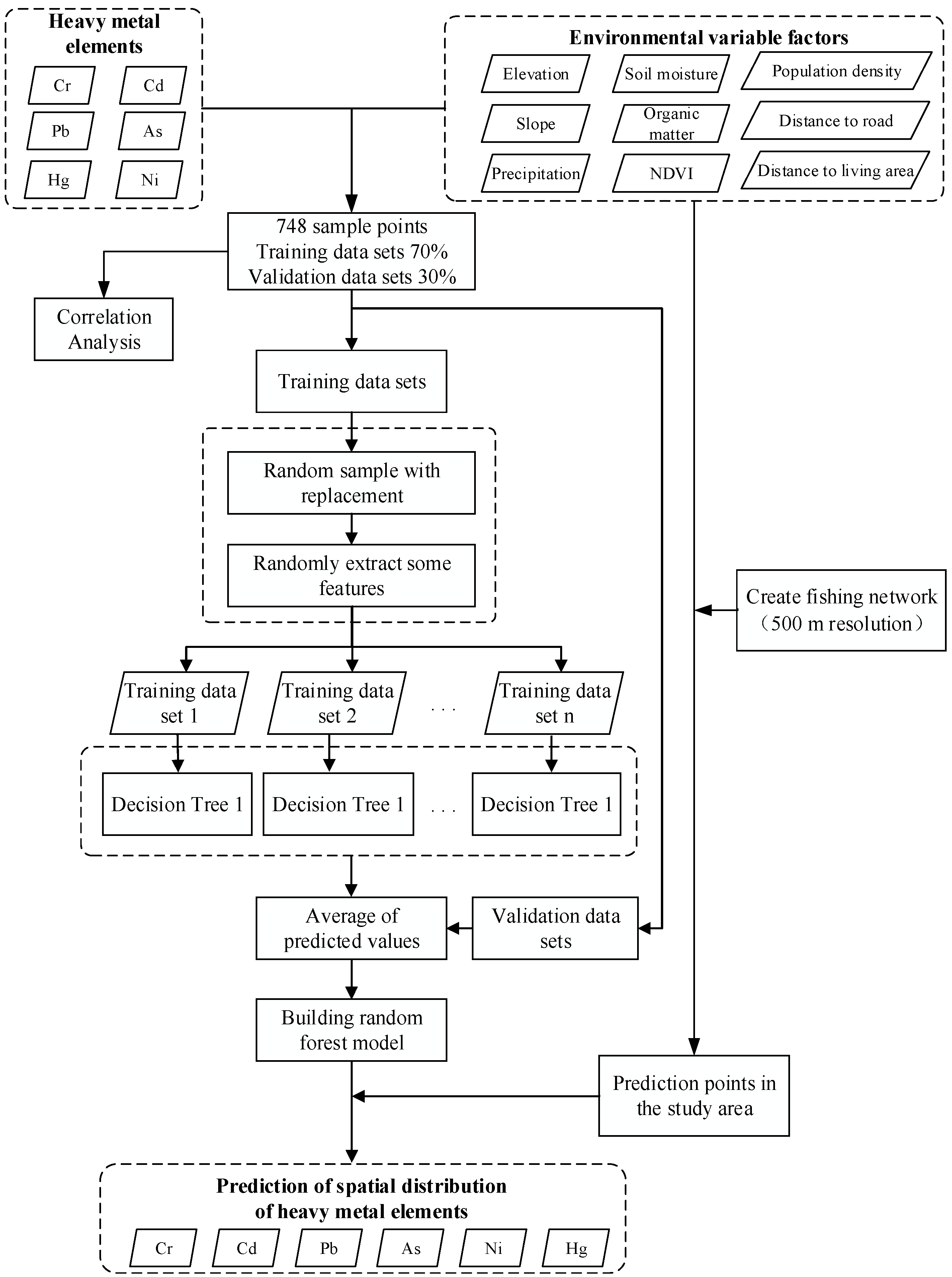
- (1)
- The environmental factor variables of the sampling points are acquired and combined with heavy metal element contents at the sampling points to form a dataset.
- (2)
- The dataset is divided into a training set and a validation set in a 7:3 ratio. The training set is used to train RF models with different parameters, and the validation set is utilized for accuracy validation to select the optimal model.
- (3)
- Construction of the RF model: Utilizing the Bootstrap resampling method, n samples are randomly drawn from the training set to form a new training sample set. With the dataset containing nine feature factors, a random subset of m (where m ≤ 9) features is selected to form a feature subset. Decision trees are constructed on the new sample set and feature subset, selecting the best splitting attribute during the tree-growing process for node splitting. This process is repeated multiple times to construct decision trees and obtain base estimators. These decision trees are then combined to form the RF.
- (4)
- Using the “Fishnet” tool in ArcGIS 10.8, a 500 m grid of points was created for the study area. The “Extract Values to Points” tool in ArcGIS 10.8 was then used to extract nine environmental covariates for the grid points.
- (5)
- The RF model was applied to predict the Cr, Cd, Pb, As, Hg, and Ni contents at each grid point. The experimental results are used to generate spatial distribution prediction maps of heavy metal elements using the “Point to Raster” tool in ArcGIS 10.8.
2.4. Parameter Settings for Random Forest Model
2.5. Accuracy Evaluation
3. Results
3.1. Statistical Characteristics of Heavy Metal Content in Soil
3.2. Correlation Analysis of Factors Affecting Heavy Metals in Soil
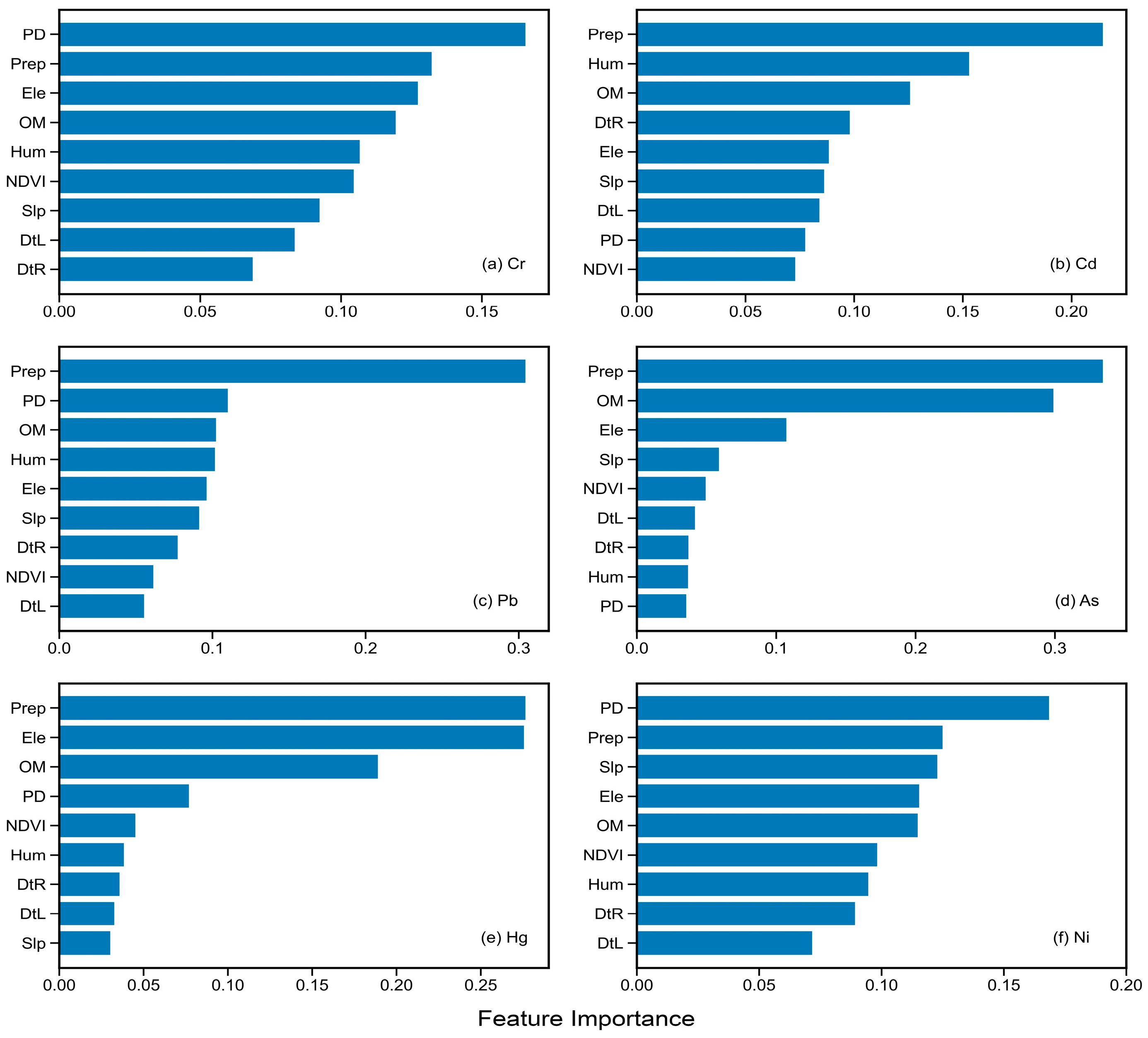
3.3. Importance Analysis of Environmental Variables in Random Forest Model
3.4. Precision Analysis of Heavy Metal Content Prediction Based on Random Forest Model
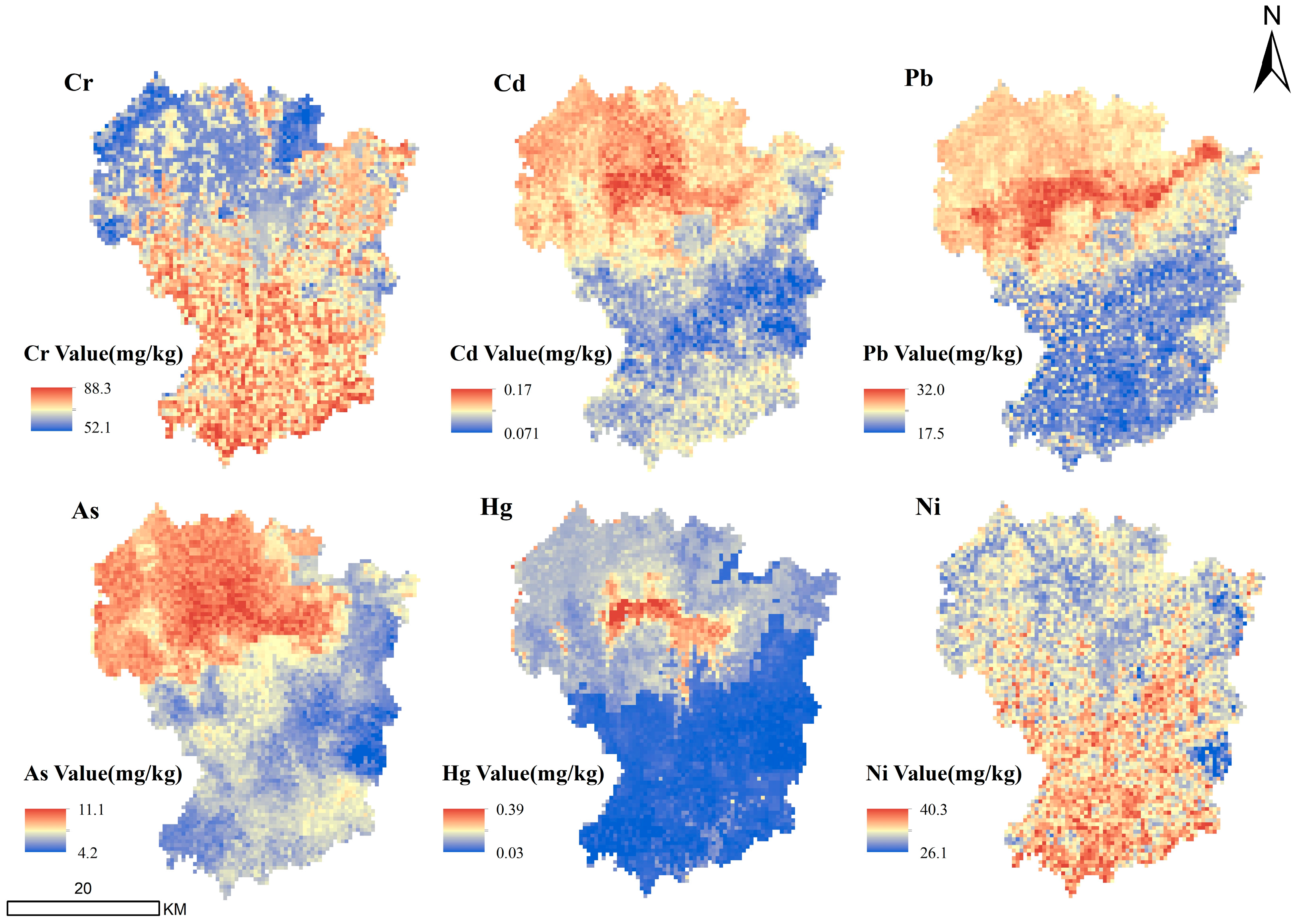
3.5. Spatial Distribution Prediction of Soil Heavy Metals Based on Random Forest Model
4. Discussion
5. Conclusions
- (1)
- The modeling results of the RF model indicate that environmental variables play a significant role in explaining the variations in the soil heavy metal content of Cr, Cd, As, Pb, Hg, and Ni within the study area. The close similarity between the R2 values of the training and validation sets suggests that the RF model exhibits reduced overfitting issues and higher stability in predicting the spatial distribution of heavy metals in the soil within the study area. Therefore, the RF model demonstrates a favorable performance in predicting the spatial distribution of soil heavy metal content.
- (2)
- For the soil heavy metal content in the study area, annual precipitation and population density are identified as major influencing factors. Specifically, Cd and Hg are primarily water-soluble components, while Cr, As, Pb, and Ni mainly exist in insoluble forms in water. Therefore, precipitation plays a significant role in soil heavy metal dynamics due to its dilution and dissolution effects. Consequently, there is a substantial relationship between precipitation and soil heavy metal content. Additionally, human activities are significant factors influencing soil heavy metal content. Hence, there is a notable correlation between population density and soil heavy metal content.
- (3)
- Based on the predicted distribution maps and the natural and social environmental conditions of the study area, it is evident that industrial activities can lead to elevated levels of Pb and Hg in the soil. The use of agricultural products in agricultural production can result in increased levels of Cd and As in the soil. Cr and Ni are primarily influenced by natural environmental factors and precipitation, with less influence from human activities.
Author Contributions
Funding
Data Availability Statement
Conflicts of Interest
References
- Gao, Q.; Yu, M.; Liu, Y.H.; Xu, H.M.; Xu, X. Modeling interplay between regional net ecosystem carbon balance and soil erosion for a crop-pasture region. J. Geophys. Res.-Biogeosci. 2007, 112. [Google Scholar] [CrossRef]
- Cuevas, J.; Daliakopoulos, I.N.; Del Moral, F.; Hueso, J.J.; Tsanis, I.K. A Review of Soil-Improving Cropping Systems for Soil Salinization. Agronomy 2019, 9, 295. [Google Scholar] [CrossRef]
- Li, G.; Sun, G.X.; Ren, Y.; Luo, X.S.; Zhu, Y.G. Urban soil and human health: A review. Eur. J. Soil Sci. 2018, 69, 196–215. [Google Scholar] [CrossRef]
- Chen, W.P.; Yang, Y.; Xie, T.; Wang, M.E.; Peng, C.; Wang, R.D. Challenges and Countermeasures for Heavy Metal Pollution Control in Farmlands of China. Acta Pedol. Sin. 2018, 55, 261–272. [Google Scholar]
- Jiao, S.; Chen, Z.H.; Yu, A.H.; Chen, H.H. Evaluation of the heavy metal pollution ecological risk in topsoil: A case study from Nanjing, China. Environ. Earth Sci. 2022, 81, 532. [Google Scholar] [CrossRef]
- Alyemeni, M.N.; Almohisen, I.A.A. Traffic and industrial activities around Riyadh cause the accumulation of heavy metals in legumes: A case study. Saudi J. Biol. Sci. 2014, 21, 167–172. [Google Scholar] [CrossRef] [PubMed]
- Cao, M.Z.; Zhu, W.J.; Hong, L.D.; Wang, W.P.; Yao, Y.L.; Zhu, F.X.; Hong, C.L.; He, S.Y. Assessing Pb-Cr Pollution Thresholds for Ecological Risk and Potential Health Risk in Selected Several Kinds of Rice. Toxics 2022, 10, 645. [Google Scholar] [CrossRef]
- Chen, H.H.; Wang, L.; Yu, A.H. Evaluation of heavy metal pollution in the soil surface of adaptive FCM—Taking the Nanjing refinery and its living area as an example. China Environ. Sci. 2022, 42, 5239–5245. [Google Scholar]
- Yaashikaa, P.R.; Kumar, P.S.; Jeevanantham, S.; Saravanan, R. A review on bioremediation approach for heavy metal detoxification and accumulation in plants. Environ. Pollut. 2022, 301, 119035. [Google Scholar] [CrossRef]
- Burges, A.; Epelde, L.; Garbisu, C. Impact of repeated single-metal and multi-metal pollution events on soil quality. Chemosphere 2015, 120, 8–15. [Google Scholar] [CrossRef]
- Li, W.J.; Yin, Z.X.; Yue, B.; Gao, T.P.; Chang, G.H. Distribution and Risk Assessment of Some Heavy Metal Elements in the Contaminated soil from Baiyin City, Gansu Province. IOP Conf. Ser. Earth Environ. Sci. 2020, 568, 012044. [Google Scholar] [CrossRef]
- Cheng, H.; Shen, R.L.; Chen, Y.Y.; Wan, Q.J.; Shi, T.Z.; Wang, J.J.; Wan, Y.; Hong, Y.S.; Li, X.C. Estimating heavy metal concentrations in suburban soils with reflectance spectroscopy. Geoderma 2019, 336, 59–67. [Google Scholar] [CrossRef]
- Xu, X.X.; Shi, F.D.; Zhu, J.J. Analyzing the critical factors influencing residents’ willingness to pay for old residential neighborhoods renewal: Insights from Nanjing, China. Environ. Dev. Sustain. 2024. [Google Scholar] [CrossRef]
- Yang, Q.; Zheng, J.Z.; Zhu, H.C. Influence of spatiotemporal change of temperature and rainfall on major grain yields in southern Jiangsu Province, China. Glob. Ecol. Conserv. 2020, 21, e00818. [Google Scholar] [CrossRef]
- Han, X.; Wu, H.; Li, Q.; Cai, W.; Hu, S. Assessment of heavy metal accumulation and potential risks in surface sediment of estuary area: A case study of Dagu river. Mar. Environ. Res. 2024, 196, 106416. [Google Scholar] [CrossRef] [PubMed]
- Jin, Z.; Lv, J.S. Comparison of the accuracy of spatial prediction for heavy metals in regional soils based on machine learning models. Geogr. Res. 2022, 41, 1731–1747. [Google Scholar]
- Mansuy, N.; Thiffault, E.; Paré, D.; Bernier, P.; Guindon, L.; Villemaire, P.; Poirier, V.; Beaudoin, A. Digital mapping of soil properties in Canadian managed forests at 250 m of resolution using the k-nearest neighbor method. Geoderma 2014, 235, 59–73. [Google Scholar] [CrossRef]
- Kuhn, M. Building predictive models in R using the caret package. J. Stat. Softw. 2008, 28, 1–26. [Google Scholar] [CrossRef]
- Henderson, B.L.; Bui, E.N.; Moran, C.J.; Simon, D.A.P. Australia-wide predictions of soil properties using, decision trees. Geoderma 2005, 124, 383–398. [Google Scholar] [CrossRef]
- Breiman, L. Random forests. Mach. Learn. 2001, 45, 5–32. [Google Scholar] [CrossRef]
- Dharumarajan, S.; Hegde, R.; Singh, S.K. Spatial prediction of major soil properties using Random Forest techniques—A case study in semi-arid tropics of South India. Geoderma Reg. 2017, 10, 154–162. [Google Scholar] [CrossRef]
- Chagas CD, S.; Junior WD, C.; Bhering, S.B.; Filho, B.C. Spatial prediction of soil surface texture in a semiarid region using random forest and multiple linear regressions. Catena 2016, 139, 232–240. [Google Scholar] [CrossRef]
- Guo, P.T.; Li, M.F.; Luo, W.; Lin, Q.H.; Tang, Q.F.; Liu, Z.W. Prediction of soil total nitrogen for rubber plantation at regional scale based on environmental variables and random forest approach. Trans. Chin. Soc. Agric. Eng. 2015, 31, 194–202. [Google Scholar]
- Ma, W.; Tan, K.; Du, P. Predicting soil heavy metal based on Random Forest model. In Proceedings of the 2016 IEEE International Geoscience and Remote Sensing Symposium (IGARSS), Beijing, China, 10–15 July 2016; pp. 4331–4334. [Google Scholar]
- Tan, K.; Wang, H.; Chen, L.; Du, Q.; Du, P.J.; Pan, C.C. Estimation of the spatial distribution of heavy metal in agricultural soils using airborne hyperspectral imaging and random forest. J. Hazard. Mater. 2020, 382, 120987. [Google Scholar] [CrossRef] [PubMed]
- Xu, J.; Xiao, P. Influence factor analysis of soil heavy metal based on categorical regression. Int. J. Environ. Sci. Technol. 2022, 19, 7373–7386. [Google Scholar] [CrossRef]
- Yang, J.; Wang, J.Y.; Qiao, P.W.; Zheng, Y.M.; Yang, J.X.; Chen, T.B.; Lei, M.; Wan, X.M.; Zhou, X.Y. Identifying factors that influence soil heavy metals by using categorical regression analysis: A case study in Beijing, China. Front. Environ. Sci. Eng. 2020, 14, 37. [Google Scholar] [CrossRef]
- Shin, H.; Yu, J.; Wang, L.; Jeong, Y.; Kim, J. Spectral Interference of Heavy Metal Contamination on Spectral Signals of Moisture Content for Heavy Metal Contaminated Soils. IEEE Trans. Geosci. Remote Sens. 2020, 58, 2266–2275. [Google Scholar] [CrossRef]
- Kou, B.; Yuan, Y.; Zhu, X.; Ke, Y.; Wang, H.; Yu, T.Q.; Tan, W.B. Effect of soil organic matter-mediated electron transfer on heavy metal remediation: Current status and perspectives. Sci. Total Environ. 2024, 917, 170451. [Google Scholar] [CrossRef]
- Zeng, F.; Ali, S.; Zhang, H.; Ouyang, Y.N.; Qiu, B.Y.; Wu, F.B.; Zhang, G.P. The influence of pH and organic matter content in paddy soil on heavy metal availability and their uptake by rice plants. Environ. Pollut. 2011, 159, 84–91. [Google Scholar] [CrossRef]
- Cao, J.; Xie, C.Y.; Hou, Z.R. Transport patterns and numerical simulation of heavy metal pollutants in soils of lead–zinc ore mines. J. Mt. Sci. 2021, 18, 2345–2356. [Google Scholar] [CrossRef]
- Zhu, P.; Cui, S.S.; Li, Z.T.; Zhu, X.T.; He, J.L.; Tan, H. Influence of Atmospheric Precipitation on the Release of Cadmium from High Background Soils in Karst Areas of Guizhou. Ecol. Environ. 2021, 30, 2213–2222. [Google Scholar]
- Ling, X.D.; Wang, L.Q.; Zhao, K.L.; Fu, W.J.; Ye, Z.Q.; Ding, L.Z. Spatial distribution characteristics of soil available nutrients in hickory plantation based on random forest method. Acta Ecol. Sin. 2024, 44, 662–675. [Google Scholar]
- He, M.Y.; Dong, J.B.; Jin, Z.; Liu, C.Y.; Xiao, J.; Zhang, F.; Sun, H.; Zhao, Z.Q.; Gou, L.F.; Liu, W.G.; et al. Pedogenic processes in loess-paleosol sediments: Clues from Li isotopes of leachate in Luochuan loess. Geochim. Et Cosmochim. Acta 2021, 299, 151–162. [Google Scholar] [CrossRef]
- Bai, B.; Xu, T.; Nie, Q.; Li, P.P. Temperature-driven migration of heavy metal Pb2+ along with moisture movement in unsaturated soils. Int. J. Heat Mass Transf. 2020, 153, 119573. [Google Scholar] [CrossRef]
- Dai, Q.Q.; Xu, M.J.; Zhuang, S.Y.; Chen, D.F. Study on Factors Influencing Heavy Metal of Farmland Soils Based on Geographical Detector in Fengqiu County. Soils 2022, 54, 564–571. [Google Scholar]
- Guo, G.H.; Lei, M.; Chen, T.B.; Song, B.; Li, X.Y. Effect of road traffic on heavy metals in road dusts and roadside soils. Acta Sci. Circumstantiae 2008, 28, 1937–1945. [Google Scholar]
- Liu, P.J.; Wu, K.N.; Luo, N. Potential Risk Factors Identification of Heavy Metals Spatial Variation in Typical Agricultural Land Topsoil of Taihu Basin. Resour. Environ. Yangtze Basin 2020, 29, 609–622. [Google Scholar]
- GB 15618-2018; Soil environmental quality Risk control standard for soil contamination of agricultural land. Standardization Administration: Beijing, China, 2018.
- Ding, Y.X.; Peng, S.Z. Spatiotemporal Trends and Attribution of Drought across China from 1901–2100. Sustainability 2020, 12, 477. [Google Scholar] [CrossRef]
- Li, Q.L.; Shi, G.S.; Shangguan, W.; Nourani, V.; Li, J.D.; Li, L.; Huang, F.N.; Zhang, Y.; Wang, C.Y.; Wang, D.G.; et al. A 1 km daily soil moisture dataset over China using in situ measurement and machine learning. Earth Syst. Sci. Data 2022, 14, 5267–5286. [Google Scholar] [CrossRef]
- Yang, J.; Dong, J.; Xiao, X.; Dai, J.; Wu, C.; Xia, J.; Zhao, G.; Zhao, M.; Li, Z.; Zhang, Y.; et al. Divergent shifts in peak photosynthesis timing of temperate and alpine grasslands in China. Remote Sens. Environ. 2019, 233, 111395. [Google Scholar] [CrossRef]
- Tatem, A.J. WorldPop, open data for spatial demography. Sci. Data 2017, 4, 170004. [Google Scholar] [CrossRef] [PubMed]
- Lu, H.L.; Zhao, M.S.; Liu, B.Y.; Zhang, P.; Lu, L.M. Spatial Prediction of Soil Properties Based on Random Forest Model in Anhui Province. Soils 2019, 51, 602–608. [Google Scholar]
- Zhao, C.; Wang, Q.; Dai, J.P. Investigation and analysis of background value of heavy metals in soil of Shandong Province. Environ. Prot. Sci. 2021, 47, 117–121. [Google Scholar]
- Song, J.Q.; Zhu, Q.; Jiang, X.S.; Zhao, H.Y.; Liang, Y.H.; Luo, Y.X.; Wang, Q.; Zhao, L.L. GIS-Based Heavy Metals Risk Assessment of Agricultural Soils—A Case Study of Baguazhou, Nanjing. Acta Pedol. Sin. 2017, 54, 81–91. [Google Scholar]
- Zhou, Y.F.; Xie, B.L.; Li, M.S. Mapping regional forest aboveground biomass from random forest Co-Kriging approach: A case study from north Guangdong. J. Nanjing For. Univ. (Nat. Sci. Ed.) 2023, 48, 169–178. [Google Scholar]
- Chen, Y.C.; Duan, W.T.; Chi, Y.H.; Li, P.; Liu, H. Study on County Village Type Identification Under the Background of Urban–rural Integration Development: A Case Study of Zhaoyuan City in Shandong Province. Urban Dev. Stud. 2022, 29, 28–37. [Google Scholar]
- Li, Z.Y.; Ma, Z.W.; Van Der Kuijp, T.J.; Yuan, Z.W.; Huang, L. A review of soil heavy metal pollution from mines in China: Pollution and health risk assessment. Sci. Total Environ. 2014, 468, 843–853. [Google Scholar] [CrossRef] [PubMed]
- Sun, X.F.; Zhang, L.X.; Dong, Y.L.; Zhu, L.Y.; Wang, Z.; Lu, J.T. Source Apportionment and Spatial Distribution Simulation of Heavy Metals in a Typical Petrochemical Industrial City. Environ. Sci. 2021, 42, 1093–1104. [Google Scholar]
- Li, Y.L.; Chen, W.P.; Yang, Y.; Wang, T.Q.; Liu, C.F.; Cai, B. Heavy metal pollution characteristics and comprehensive risk evaluation of farmland across the eastern plain of Jiyuan city. Acta Sci. Circumstantiae 2020, 40, 2229–2236. [Google Scholar]
- Ji, F.H.; Liu, J.; Wang, L.M. Summary of Remote Sensing Algorithm in Crop Type Identification and Its Application Based on Gaofen Satellites. Chin. J. Agric. Resour. Reg. Plan. 2021, 42, 254–268. [Google Scholar]
- Cheng, J.; Yuan, X.Y.; Zhang, H.Y.; Mao, Z.Q.; Zhu, H.; Wang, Y.M.; Li, J.Z. Characteristics of Heavy Metal Pollution in Soils of Yunnan-Guizhou Phosphate Ore Areas and Their Effects on Quality of Agricultural Products. J. Ecol. Rural Environ. 2021, 37, 636–643. [Google Scholar]
- Huang, H.B.; Lin, C.Q.; Hu, G.R.; Yu, R.L.; Hao, C.L.; Chen, F.H. Source Appointment of Heavy Metals in Agricultural Soils of the Jiulong River Basin Based on Positive Matrix Factorization. Environ. Sci. 2020, 41, 430–437. [Google Scholar]
- Wang, M.E.; Peng, C.; Chen, W.P. Impacts of Industrial Zone in Arid Area in Ningxia Province on the Accumulation of Heavy Metals in Agricultural Soils. Environ. Sci. 2016, 37, 3532–3539. [Google Scholar]
- Belgiu, M.; Drăguţ, L. Random forest in remote sensing: A review of applications and future directions. ISPRS J. Photogramm. Remote Sens. 2016, 114, 24–31. [Google Scholar] [CrossRef]
- Shi, G.; Liu, G.; Zhao, L.; Su, Y.Q.; Bi, R.T. Prediction of arsenic for farmland soil based on multi source environmental data and random forest model. Acta Sci. Circumstantiae 2020, 40, 2993–3000. [Google Scholar]
- Liu, Q.; Chen, W.; Wang, B.; Wang, S.; Liu, Z.Z.; Zhang, N.M.; Li, B. Contaminant Characteristics and Health Risk Assessment of Heavy Metals in Soils from Lead-Zincs Melting Plant in Huize County, Yunnan Province, China. J. Agric. Resour. Environ. 2024, 33, 221. [Google Scholar]
- Jiang, Y.F.; Huang, M.X.; Chen, X.Y.; Wang, Z.G.; Xiao, L.J.; Xu, K.; Zhang, S.; Wang, M.M.; Xu, Z.; Shi, Z. Identification and risk prediction of potentially contaminated sites in the Yangtze River Delta. Sci. Total Environ. 2022, 815, 151982. [Google Scholar] [CrossRef] [PubMed]
- Li, T.Y.; Jia, W.W.; Sun, Y.M.; Wang, H.Z.; Ma, S.Y. Analysis of Spatial Distribution of Korean Pines in Liangshui Nature Reserve Based on the Geographically Weighted Regression Model. For. Eng. 2024, 40, 47–59. [Google Scholar]
- Wang, Q.; Xie, Z.; Li, F. Using ensemble models to identify and apportion heavy metal pollution sources in agricultural soils on a local scale. Environ. Pollut. 2015, 206, 227–235. [Google Scholar] [CrossRef]
- Wang, H.; Yilihamu, Q.; Yuan, M.; Bai, H.; Xu, H.; Wu, J. Prediction models of soil heavy metal(loid)s concentration for agricultural land in Dongli: A comparison of regression and random forest. Ecol. Indic. 2020, 119, 106801. [Google Scholar] [CrossRef]
- Azizi, K.; Ayoubi, S.; Nabiollahi, K.; Garosi, Y.; Gislum, R. Predicting heavy metal contents by applying machine learning approaches and environmental covariates in west of Iran. J. Geochem. Explor. 2022, 233, 106921. [Google Scholar] [CrossRef]
- Liu, W.R.; Zeng, D.; She, L.; Su, W.X.; He, D.C.; Wu, G.Y.; Ma, X.R.; Jiang, S.; Jiang, C.H.; Ying, G.G. Comparisons of pollution characteristics, emission situations, and mass loads for heavy metals in the manures of different livestock and poultry in China. Sci. Total Environ. 2020, 734, 139023. [Google Scholar] [CrossRef] [PubMed]


| Name of Indicators | Unit | Data Sources | Calculation Method |
|---|---|---|---|
| Elevation | m | www.gscloud.cn (accessed on 1 October 2023) | / |
| Slope | degree | www.gscloud.cn | / |
| Precipitation | mm | https://doi.org/10.5281/zenodo.3185722 (accessed on 1 October 2023) | / |
| Humidity | dm3/m3 | https://cstr.cn/18406.11.Terre.tpdc.272415 (accessed on 1 October 2023) | / |
| Organic Matter | mg/kg | https://doi.org/10.11888/Soil.tpdc.270281 (accessed on 1 October 2023) | / |
| NDVI | / | https://cstr.cn/15732.11.nesdc.ecodb.rs.2021.012 (accessed on 1 October 2023) | / |
| Distance to Living Area | m | / | The distance from sampling points to residential areas is calculated based on the land use type by a “proximity analysis” in ArcGIS 10.8. |
| Distance to Road | m | https://www.openstreetmap.org (accessed on 1 October 2023) | The distance from sampling points to roads is calculated by a “proximity analysis” in ArcGIS 10.8. |
| Population Density | person/km2 | www.worldpop.org (accessed on 1 October 2023) | / |
| ntree | max_ Depth | Cr | Cd | Pb | ||||
| Training Set (R2) | Validation Set (R2) | Training Set (R2) | Validation Set (R2) | Training Set (R2) | Validation Set (R2) | |||
| Test 1 | 500 | 10 | 0.556 | 0.507 | 0.517 | 0.496 | 0.521 | 0.511 |
| 500 | 20 | 0.599 | 0.539 | 0.518 | 0.498 | 0.527 | 0.521 | |
| 500 | 30 | 0.599 | 0.538 | 0.516 | 0.497 | 0.526 | 0.520 | |
| Test 2 | 800 | 10 | 0.559 | 0.508 | 0.517 | 0.499 | 0.522 | 0.517 |
| 800 | 20 | 0.600 | 0.542 | 0.523 | 0.504 | 0.535 | 0.527 | |
| 800 | 30 | 0.600 | 0.541 | 0.522 | 0.503 | 0.534 | 0.526 | |
| Test 3 | 1000 | 10 | 0.558 | 0.507 | 0.517 | 0.498 | 0.521 | 0.517 |
| 1000 | 20 | 0.599 | 0.540 | 0.521 | 0.501 | 0.534 | 0.524 | |
| 1000 | 30 | 0.599 | 0.540 | 0.520 | 0.500 | 0.533 | 0.523 | |
| ntree | max_ Depth | As | Hg | Ni | ||||
| Training Set (R2) | Validation Set (R2) | Training Set (R2) | Validation Set (R2) | Training Set (R2) | Validation Set (R2) | |||
| Test 1 | 500 | 10 | 0.622 | 0.618 | 0.605 | 0.573 | 0.473 | 0.454 |
| 500 | 20 | 0.627 | 0.622 | 0.607 | 0.579 | 0.511 | 0.481 | |
| 500 | 30 | 0.626 | 0.621 | 0.606 | 0.578 | 0.510 | 0.480 | |
| Test 2 | 800 | 10 | 0.629 | 0.625 | 0.610 | 0.582 | 0.472 | 0.452 |
| 800 | 20 | 0.631 | 0.627 | 0.612 | 0.584 | 0.512 | 0.482 | |
| 800 | 30 | 0.630 | 0.626 | 0.611 | 0.583 | 0.511 | 0.481 | |
| Test 3 | 1000 | 10 | 0.627 | 0.624 | 0.609 | 0.581 | 0.475 | 0.453 |
| 1000 | 20 | 0.628 | 0.625 | 0.610 | 0.582 | 0.509 | 0.481 | |
| 1000 | 30 | 0.625 | 0.621 | 0.610 | 0.579 | 0.510 | 0.480 | |
| Metal | Range (mg/kg) | Mean Value (mg/kg) | Standard Deviation (mg/kg) | Skewness | Kurtosis | Coefficient of Variation (%) | Background Value [45] (mg/kg) |
|---|---|---|---|---|---|---|---|
| Cr | 12.70~144.00 | 57.01 | 20.62 | 1.56 | 2.96 | 36.17 | 57 |
| Cd | 0.0031~0.30 | 0.12 | 0.059 | 0.68 | 0.35 | 49.17 | 0.117 |
| Pb | 6.87~57.80 | 23.40 | 7.22 | 0.73 | 1.81 | 30.85 | 27.2 |
| As | 2.37~21.80 | 7.65 | 2.51 | 1.00 | 3.57 | 32.81 | 6.4 |
| Hg | 0.011~1.05 | 0.072 | 0.10 | 4.99 | 32.06 | 138.89 | 0.034 |
| Ni | 4.07~82.80 | 27.74 | 11.03 | 1.13 | 1.34 | 39.76 | 24.6 |
| Metal | Range (mg/kg) | Mean Value (mg/kg) | Standard Deviation (mg/kg) | Skewness | Kurtosis | Coefficient of Variation (%) | Background Value [45] (mg/kg) |
|---|---|---|---|---|---|---|---|
| Cr | 6.39~147.00 | 58.35 | 24.36 | 1.33 | 2.07 | 41.75 | 57 |
| Cd | 0.0161~0.29 | 0.12 | 0.060 | 0.68 | 0.20 | 50.00 | 0.117 |
| Pb | 8.25~56.30 | 23.23 | 6.82 | 0.98 | 2.35 | 29.36 | 27.2 |
| As | 2.22~21.80 | 7.24 | 2.58 | 1.32 | 5.50 | 35.64 | 6.4 |
| Hg | 0.014~0.95 | 0.058 | 0.065 | 4.29 | 22.68 | 112.07 | 0.034 |
| Ni | 6.07~81.80 | 28.03 | 11.99 | 0.88 | 0.24 | 42.78 | 24.6 |
| Variable | Cr | Cd | Pb | As | Hg | Ni |
|---|---|---|---|---|---|---|
| Organic Matter | −0.028 | 0.226 ** | 0.208 ** | 0.504 ** | 0.349 ** | −0.030 |
| Precipitation | 0.150 ** | −0.188 ** | −0.218 ** | −0.288 ** | −0.224 ** | 0.107 ** |
| Humidity | 0.022 | −0.055 | −0.041 | −0.034 | −0.062 | −0.001 |
| Elevation | 0.133 ** | −0.233 ** | −0.253 ** | −0.516 ** | −0.374 ** | 0.081 * |
| Slope | −0.084 * | 0.033 | 0.099 ** | 0.044 | 0.039 | −0.056 |
| NDVI | 0.041 | −0.058 | −0.026 | −0.056 * | 0.026 | −0.004 |
| Distance to Living Area | 0.012 | −0.115 ** | −0.102 ** | −0.227 ** | −0.152 ** | 0.011 |
| Distance to Road | −0.002 | −0.025 | −0.007 | 0.038 | 0.058 * | 0.045 |
| Population Density | −0.159 ** | 0.144 ** | 0.229 ** | 0.233 ** | 0.299 ** | −0.122 ** |
| Element | Training Datasets | Validation Datasets | ||||
|---|---|---|---|---|---|---|
| RMSE (mg/kg) | MAE (mg/kg) | R2 | RMSE (mg/kg) | MAE (mg/kg) | R2 | |
| Cr | 3.840 | 10.200 | 0.600 | 4.055 | 11.943 | 0.542 |
| Cd | 0.190 | 0.028 | 0.523 | 0.205 | 0.032 | 0.504 |
| Pb | 2.047 | 2.952 | 0.535 | 2.164 | 3.402 | 0.527 |
| As | 1.168 | 0.945 | 0.631 | 1.254 | 1.023 | 0.627 |
| Hg | 0.241 | 0.023 | 0.612 | 0.205 | 0.021 | 0.584 |
| Ni | 2.693 | 5.388 | 0.512 | 2.935 | 6.559 | 0.482 |
Disclaimer/Publisher’s Note: The statements, opinions and data contained in all publications are solely those of the individual author(s) and contributor(s) and not of MDPI and/or the editor(s). MDPI and/or the editor(s) disclaim responsibility for any injury to people or property resulting from any ideas, methods, instructions or products referred to in the content. |
© 2024 by the authors. Licensee MDPI, Basel, Switzerland. This article is an open access article distributed under the terms and conditions of the Creative Commons Attribution (CC BY) license (https://creativecommons.org/licenses/by/4.0/).
Share and Cite
Nie, S.; Chen, H.; Sun, X.; An, Y. Spatial Distribution Prediction of Soil Heavy Metals Based on Random Forest Model. Sustainability 2024, 16, 4358. https://doi.org/10.3390/su16114358
Nie S, Chen H, Sun X, An Y. Spatial Distribution Prediction of Soil Heavy Metals Based on Random Forest Model. Sustainability. 2024; 16(11):4358. https://doi.org/10.3390/su16114358
Chicago/Turabian StyleNie, Shunqi, Honghua Chen, Xinxin Sun, and Yunce An. 2024. "Spatial Distribution Prediction of Soil Heavy Metals Based on Random Forest Model" Sustainability 16, no. 11: 4358. https://doi.org/10.3390/su16114358
APA StyleNie, S., Chen, H., Sun, X., & An, Y. (2024). Spatial Distribution Prediction of Soil Heavy Metals Based on Random Forest Model. Sustainability, 16(11), 4358. https://doi.org/10.3390/su16114358