Evaluation of Traffic Efficiency and Energy-Saving Benefits of L3 Smart Vehicles under the Urban Expressway Scenario

Abstract

An L3 smart vehicle (L3 SV) could behave differently from human-driven vehicles due to its intelligent configuration and decision-making logic, and may consequently exert influences on traffic flow. In order to clarify the L3 SV’s traffic impacts and accelerate L3 SV implementation, this paper conducted an evaluation on the traffic efficiency and energy consumption influences of L3 SVs based on a microscopic traffic simulation. Taking Beijing as a case, the relevant traffic economic benefits were calculated with the help of the previously proposed traffic economic benefits model. Before modeling L3 SVs, a two-dimensional general modeling architecture for SVs was proposed. According to the architecture, the driving behavior model, as well as behavior selection models of L3 SVs, was eventually determined, based on which the intelligent driving model of L3 SVs was established. Urban expressways were selected as the simulation road type, and scenario analysis was conducted on various proportions of L3 SVs and L3 connected and autonomous vehicles (L3 CAVs), as well as the input traffic flow rates. It was found that L3 SVs can significantly reduce the travel time and energy consumption and enlarge the actual road capacity. The improvement will become particularly prominent under saturated or supersaturated traffic flow and increasing the proportion of L3 SVs and L3 CAVs can also amplify the effect of traffic optimization. The related economic benefit is considerable, which is CNY 3.104 billion a year based on Beijing’s travel and traffic conditions.

1. Introduction

Nowadays, with the rapid growth of car ownership, traffic congestion has become increasingly severe in China. A large amount of time is spent on commuting, resulting in serious time-related economic losses. It is reported that the annual congestion cost per capita in Beijing was as high as CNY 4013 in 2017 [1]. Furthermore, traffic jam increases the acceleration and deceleration conditions, as well as the idle conditions of vehicles, contributing to additional energy consumption and toxic and greenhouse gas emissions. According to International Energy Agency statistics, China’s carbon emissions from transportation in 2022 were 1.26 billion tons, over 80% of which were made up of road transportation emissions [2]. In other words, road transportation carbon emissions account for approximately 8.32% of that of the whole country. Low traffic efficiency is bound to further increase these figures.

An Intelligent Transportation System (ITS) is regarded as one of the most efficient ways to improve traffic efficiency and save traffic energy consumption [3,4]. Different kinds of advanced technologies are applied to different transportation participants, in order to bridge the information gap between them, enhance their intelligence levels, and build up a new transportation system eventually with higher security and efficiency [3]. Smart vehicles (SVs) are an important component of an ITS [5,6,7]. It is not only a new kind of vehicle product but also a tool to optimize the traffic operation status. There are two main kinds of SVs according to the technical route [6,8]. One is the autonomous vehicle (AV). It is equipped with sensors, high-performance computing platforms, and wire-controlled actuators, with the ability to assist or even replace human drivers to complete the driving tasks. Another one is the connected and autonomous vehicle (CAV). It adds vehicle communication modules to an AV, making it possible to communicate with other terminals (vehicle to everything, V2X) like CAVs (V2V), roadside infrastructure (V2I), cloud platforms (V2N), and even pedestrians (V2P). As a result, over-the-horizon perception information, as well as traffic information, can be provided, and driving tasks are able to be completed both by the vehicle system and the cloud control platform. In addition, SVs can also receive traffic control instructions from roadside and cloud platforms. Thus, in areas such as ramp merging and diverging, intersections, and even the entire road network, SVs can collaborate and coordinate with each other to further optimize the traffic flow.

SVs are divided into five levels according to their ability to drive autonomously [9]. This paper focused on SVs with level 3 automation (L3 SVs), which are treated as a transitional form between vehicles with primary-level and advanced-level automation. Compared with human-driven vehicles (HVs), they operate with clearer decision-making logic without any ambiguity and differences in driving styles, contributing to better performance in speed, time headway, and acceleration control. In comparison with vehicles with primary-level automation, L3 SVs have a complete capability of longitudinal and lateral perception, decision-making, and execution capabilities [9]. Furthermore, their operational design domain (simplified as ODD) is expanded compared to that of primary-level automation, in which scenarios such as autonomous lane change, ramp merging, and ramp diversion are involved. As for vehicles with advanced-level automation, L3 SVs are their base and nearly similar to them in terms of longitudinal and lateral driving capabilities but have an ODD with more limitations. For instance, the present products of L3 SVs are not suitable for urban arterials and minor arterials and may be faced with much more corner cases that are hard to handle.

L3 SVs are no longer a new concept but are gradually integrating into people’s lives [10]. At present, new automotive products with so-called “level 2 plus (L2+) automation” are generally equipped with smart driving systems represented by “Navigate on Autopilot (NOA)”. NOA can assist drivers in completing longitudinal and lateral driving tasks in certain situations such as highways and urban expressways. Taking over is still necessary when the driving condition is out of the operational design domain. In fact, so-called L2+ SVs have already had the ability of L3 automation referring to the standard of vehicle automation level [9]. However, to avoid being held responsible for potential traffic accidents and limited by the current laws and policies, original equipment manufacturers (OEMs) prefer to adopt the so-called “L2+” definition, where the completion of driving tasks is still assigned to human drivers. The market penetration of L2+ SVs is rapidly increasing. It was reported that the value in China from January to October of 2023 had reached 7.6%, representing a year-on-year growth of 69% [11,12]. Recently, the four ministries of China jointly issued a notice to approve the piloting of L3 vehicles with access permits in limited areas [13]. This is undoubtedly a major benefit for the promotion of L3 vehicles, as their road use will be legalized. Thus, it can be predicted that L3 SVs will probably soon become the focus of OEMs’ recent product launches.

In summary, considering the unique driving behavior and good market development trend, it can be speculated that L3 SVs will probably exert impacts on traffic flow and are expected to be applied to traffic management to improve traffic efficiency and save traffic energy consumption. However, there are still many city governments and OEMs struggling with the methods to efficiently develop L3 SVs. The economic benefits from the traffic impacts of SVs are crucial for making their technology roadmap, promoting their widespread application, and formulating relevant business models. But there is still a lack of results. Therefore, it is of great significance to conduct a quantitative evaluation of the traffic impacts of L3 SVs.

There are currently a large number of studies on the impacts of SVs on traffic flow. Different kinds of vehicle functions, as well as boundary conditions such as road types, traffic flow rate, and traffic flow composition, are combined. A large number of researchers have focused on AVs and studied the related traffic impacts of longitudinal advanced driving assistance systems (ADASs). Klunder et al. found that the switching process of adaptive cruise control (ACC) would increase traffic delays under free flow and congested flow conditions while traffic delays could be reduced by 50% under congested flow conditions when the penetration rate of ACC reaches 100% [14]. Song et al. announced that a single-lane autonomous driving system can improve the actual road capacity, reduce travel time and traffic carbon dioxide emissions [15]. Carrone et al. found similar conclusions in a highway scenario, namely, that as the penetration rate of AVs with longitudinal automatic control capabilities increases from 0 to 100%, the average travel time decreases by nearly 50%, and the actual road capacity increases by 28% [16]. Song et al. and Stogios et al. both found that appropriately increasing the aggressiveness of ADAS can reduce transportation carbon dioxide emissions when autonomous vehicles reach a certain penetration rate [15,17]. Some scholars have also considered the influences of V2X on ADAS. Kuang et al. claimed that urban road travel time could be significantly reduced by 36.28% and the average traffic flow speed could be improved by 56.65% when the penetration rate of the cooperative ACC reaches 100%. The optimization of traffic efficiency is particularly significant during morning and evening peak hours on urban roads but is insignificant for highways and rural roads [18]. Ding proposed an autonomous lane-changing decision-making algorithm for SVs consisting of two parts: single-vehicle lane-changing decision making and collaborative lane-changing decision making. It was found that this algorithm could apparently improve traffic flow efficiency [19]. Ruan et al. compared three different information flow topologies applied to cooperative adaptive cruise control and found that multiple-predecessor-leader following could improve traffic safety and capacity most significantly as long as the communication bandwidth is sufficient [20]. Makridis et al. claimed that SVs realized by vehicles themselves would harm traffic efficiency, while SVs based on V2X could enlarge the road capacity even though the traffic carbon dioxide emissions would consequently increase [21]. In terms of the intelligent traffic management strategies based on V2X, Chou et al. proposed a V2V-based collaborative on-ramp merging mechanism for SVs and demonstrated that it could improve the road traffic capacity of merging sections even when the penetration of SVs is low [22]. Olsson and Levin proposed a V2I-based automatic intersection management strategy to ensure that they can pass the intersection without stopping. It was found that this strategy can reduce delays and increase the average travel speed of intersections [23]. Lu et al. also proposed a vehicle control strategy at continuous signal-controlled intersections based on V2I. It was illustrated that this strategy can reduce fuel consumption and carbon dioxide emissions by more than 18% on urban roads with medium traffic flow density [24]. Ma et al. studied the impact of dedicated lanes for autonomous driving on traffic efficiency in a highway scenario where CAVs and HVs mix in the traffic flow. Based on the analysis results, recommendations were provided for setting up dedicated lanes for intelligent connected vehicles under different CAV penetration rates and input traffic flow rates [25]. Song et al. found that under saturated and supersaturated traffic conditions, providing a proper number of dedicated lanes for L2 CAVs on urban expressways according to their penetration rate could remarkably amplify the improvement in traffic efficiency and reduction in energy consumption [26]. There are also a few studies that have studied the traffic impacts of SVs from the perspective of vehicle automation levels. Miqdady’s team conducted a series of studies on the traffic safety impacts of SVs with different automation levels from L1 to L4. It was announced that the severity of traffic conflicts could be significantly mitigated if the penetration rates of L3 and L4 SVs are above 55% [27], and the number of traffic conflicts would gradually decrease with the increase in the penetration rate of SVs, the range of which varies from 18.9% when the total penetration rate of L3 and L4 is 5% to 94.1% if the traffic flow is completely made up L4 SVs [28]. Furthermore, the safety influence of dedicated lanes of SVs was also analyzed. It was recommended that it was the optimal strategy to employ an SV lane under unsaturated traffic flow when the total penetration rate of L3 and L4 exceeds 55%, or under congested traffic flow no matter what the penetration rate is [29].

However, there are still some shortcomings in current research. First, most research focuses on a specific intelligent function, such as ACC and CACC, etc., but there has been relatively little research on traffic impact evaluation for SVs with different automation levels. Even though some researchers have conducted relevant studies, the driving behavior modeling of SVs with different intelligent driving levels lacks scientific methodology. Their established models have strong relevance for research purposes rather than being based on the essence of their driving behavior features. Second, the scenarios considered in most current research are too idealized or simple to reflect real traffic conditions, making the results lack authenticity, reliability, and a reference value. Third, almost all research results are just about the traffic influences rather than stepping into the relevant economic benefits. Thus, it is hard to explore the comprehensive effectiveness of SVs by combining their technical effect with their costs.

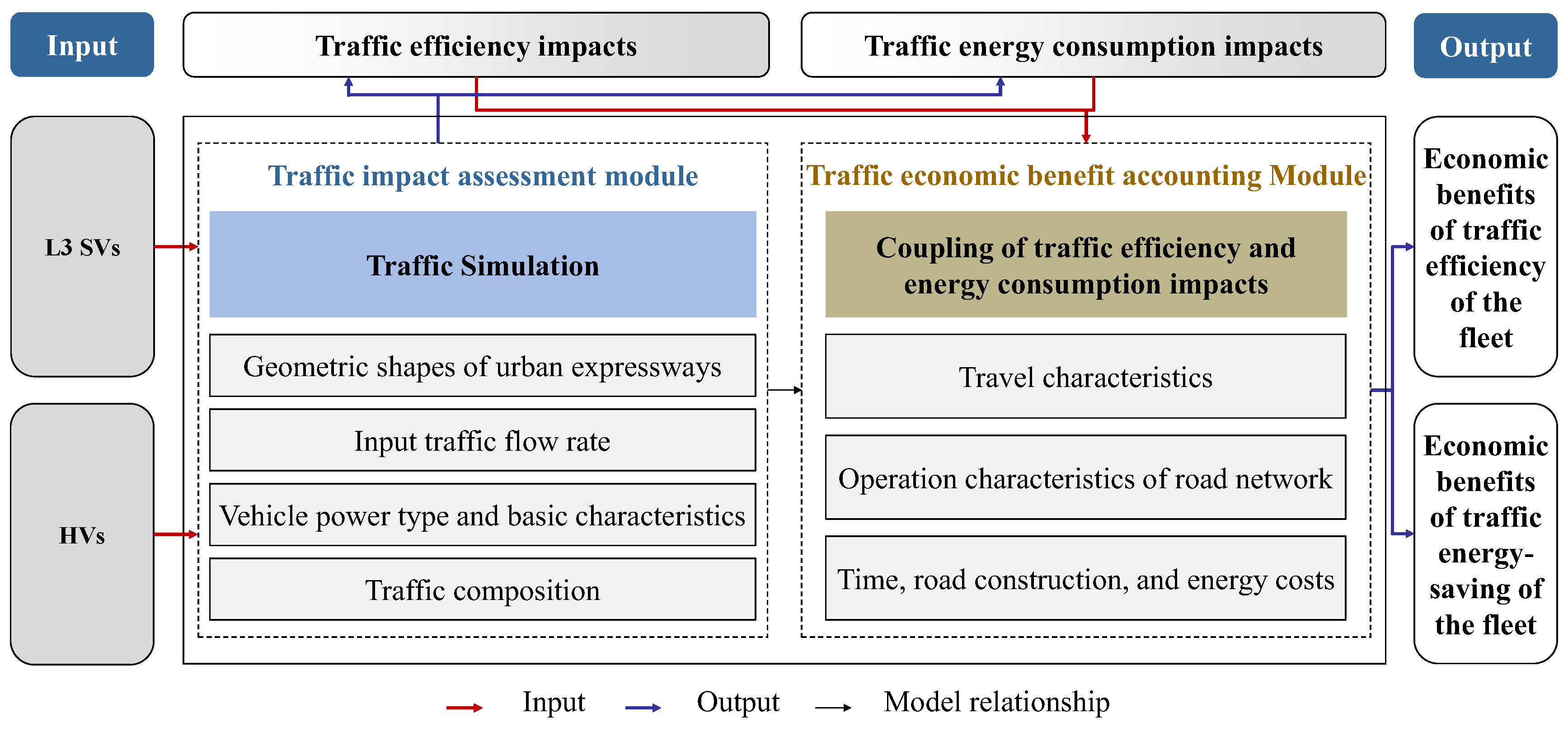
Therefore, in this study, a structure was innovatively proposed for modeling the driving behavior of SVs with different intelligence levels under the premise of rule-based algorithms, based on which the reference model of L3 SVs’ driving behavior was constructed. Next, L3 SVs’ impacts on traffic efficiency and energy consumption were evaluated under scientific scenarios through a microscopic traffic simulation. The urban expressway was chosen as the research scenario because it is the most typical kind of road suitable for L3 SVs. It makes up the least part of the whole urban road network but services the largest travel distance of the urban fleet, leading to a high traffic volume, especially in peak periods. Moreover, to support the comprehensive evaluation of SVs, a traffic economic benefit model established by the authors before was used to transfer SVs’ traffic impacts into economic indexes. This research’s results can not only reveal L3 SVs’ traffic impacts but also provide references for SV design, transportation infrastructure upgrades, and ITS development strategy making.

2. Research Roadmap

2.1. Overall Research Roadmap

The input, modules, and output of this study, as well as their relationships, are shown in Figure 1. The structure is divided into two stages. In the first stage, L3 SVs and HVs are input into the traffic impact assessment module, in which a series of traffic simulations are conducted considering the geometric shapes of urban expressways, input traffic flow rates, vehicle power types and basic characteristics, and traffic compositions. VISSIM was selected as the simulation platform, which is one of the most often-used microscopic traffic simulation software in the world [30]. The simulation settings in this research are explained in detail in Section 4. After the simulations, the traffic efficiency and energy consumption impact of L3 SVs are output as the base of traffic economic benefits calculation. In the second stage, the output of the first stage is input into the traffic economic benefits accounting module, where L3 SVs’ traffic impacts are coupled with travel characteristics, operation status of the road network, as well as time, road construction, and energy costs. Different values of these parameters can reflect the differences between different regions, cities, and even countries, which means the proposed structure has good geographical adaptability. Eventually, the traffic economic benefits of L3 SVs at the fleet level are calculated.

2.2. Framework of Traffic Impacts Evaluation

The more accurate the traffic impact results, the more reliable the traffic economic benefits are. Therefore, a general framework for the evaluation of SVs’ traffic impacts was constructed, as depicted in Figure 2. As explained before, intelligent driving can be realized by the vehicle itself or by V2X. Thus, the intelligence level of vehicles and roads should be the two main variables. Different intelligence driving levels of SVs are reflected by their driving behaviors involving two longitudinal driving behaviors and two lateral driving behaviors. The differences in various driving behaviors ultimately manifest in the decision-making logic and output decision variables. As for the roadside, corresponding to SVs, there is no harm in calling the roads equipped with intelligent transportation infrastructures smart roads (SRs). Referring to the “Technology Roadmap for Energy Saving and Nev Energy Vehicles 2.0” (simplified as “Roadmap 2.0”) [8], there are three intelligence levels of SRs. The primary-level SRs share some traffic information with vehicles like the weather, traffic accidents, etc. The medium-level SRs can assist or even substitute SVs to complete the sensing tasks except for information sharing. The advanced-level SRs can not only cover the ability of medium-level SRs but also make decisions for vehicles or the whole traffic system. In conclusion, SRs with different intelligence levels can be distinguished by their functions including supporting V2X autonomous driving and systematic traffic control. The second one can be divided into two parts according to the function range, which includes mesoscopic and macroscopic traffic control. The former usually acts on specific road areas, such as ramps and intersections, while the latter generally serves the whole road network. All SRs’ functions will eventually affect vehicles’ driving behavior and exert impacts on traffic flow. Thus, it is at the core of traffic evaluation to establish driving models for SVs. Except for the variables, there are also two kinds of boundary conditions determining the driving environment. One is the traffic conditions, including the traffic composition and input traffic flow rate, which depicts the vehicle types and the volume of traffic flow. Another is the road type that determines the scenarios that vehicles will be faced with. The application of this framework in L3 SVs’ traffic impact assessment will be described concretely in Section 3 and Section 4.

3. Vehicle Driving Models

3.1. General Modeling Architecture of SVs

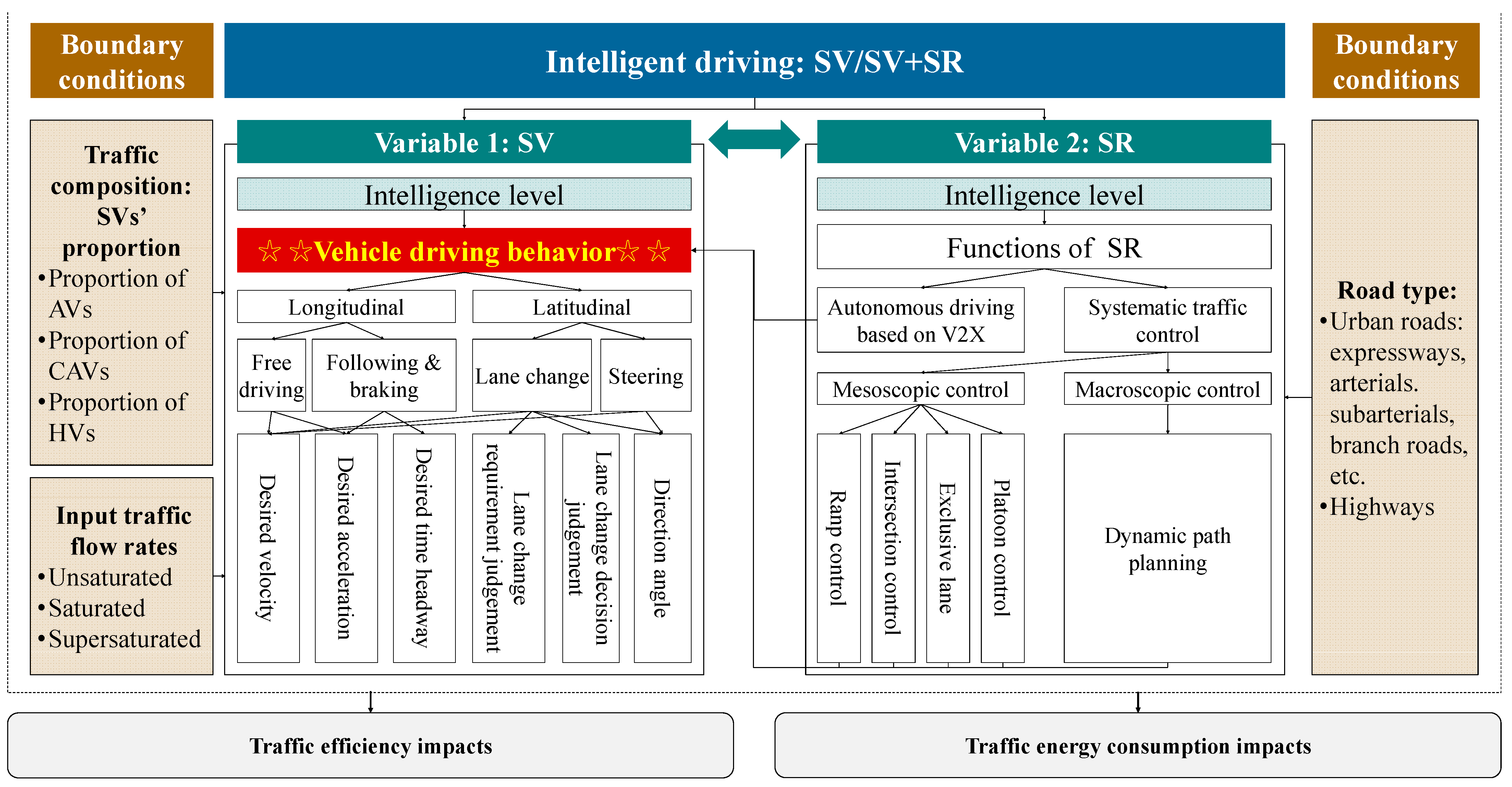
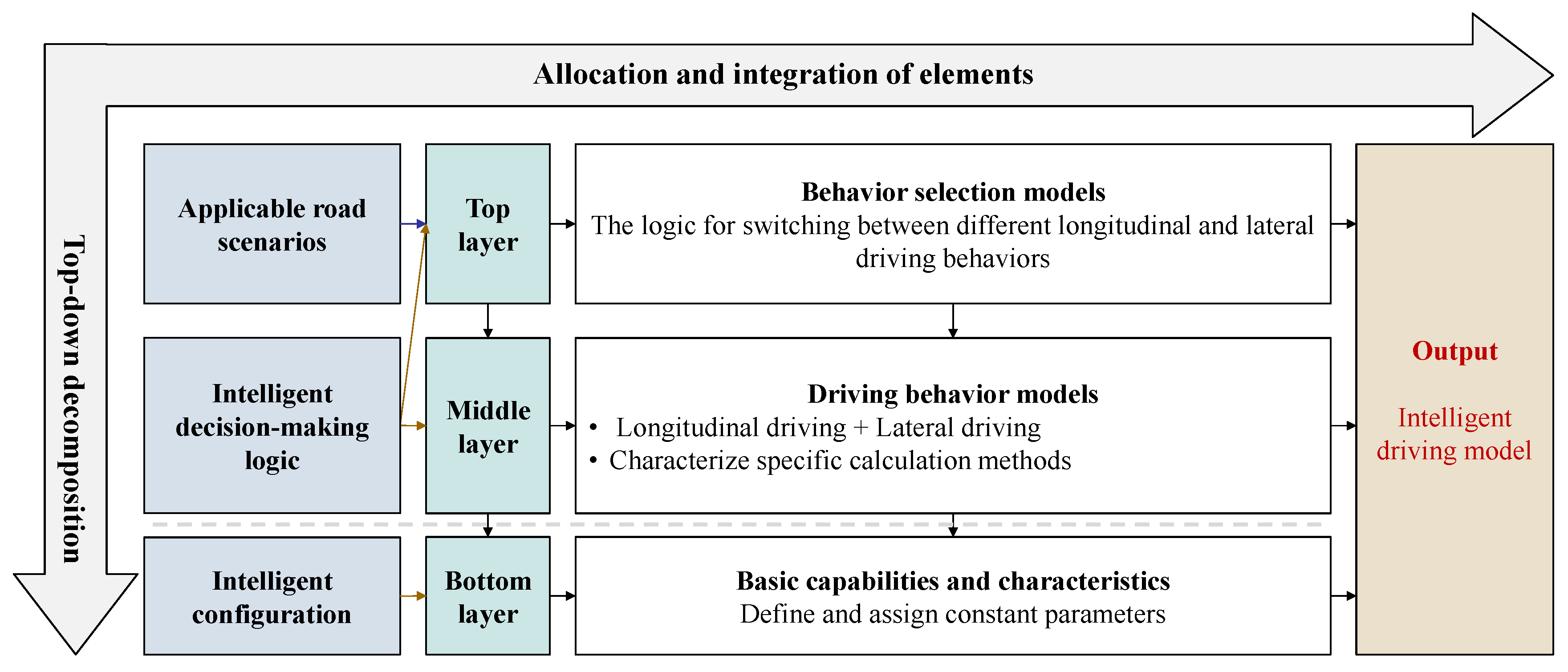
As reviewed before, there is a relatively rich variety of vehicle and traffic control models at functional levels in the current research. However, there is a lack of systematic models for SVs with different intelligent driving levels. To fill the gaps in the existing research, an innovative general modeling architecture was introduced for SVs, as depicted in Figure 3. It can be interpreted from vertical and lateral dimensions. On the vertical dimension, it is portioned into three layers from top to bottom. The top layer, similar to the human brain, represents the behavior selection models applied to define the principles for selecting and switching different longitudinal and lateral driving behaviors depending on the traffic environment as well as the mesoscopic and macroscopic traffic control. The middle layer, like the human cerebellum, is made up of driving behavior models including longitudinal and lateral models. The former is composed of free driving, vehicle following, and emergency braking, while the latter involves lane change and steering. SVs with different intelligent driving levels and technology routes can be characterized by behavior selection logic, and derivation logic of control variables in a certain driving model. The bottom layer is used to depict SVs’ basic capabilities and characteristics. They are typically defined through constant parameters in the model. The bottom layer reflects the capability and performance determined by hardware and driver’s preference so that it is decoupled from the other two layers.

On the lateral dimension, three crucial elements of intelligent driving are allocated to different layers. They are applicable road scenarios, intelligent decision-making logic, and intelligent configuration. Applicable road scenarios form the driving environments, mainly influencing the top layer. SVs need to choose the correct behavior model according to certain road scenarios. For example, an SV running on the far-left lane of the basic section of a three-lane urban expressway has to alter its driving state from vehicle following to lane change if the next section on its path is a ramp placed on the far-right side. Intelligent decision-making logic exists both in the top layer and the middle layer. On the one hand, mesoscopic and macroscopic traffic control functions themselves are an important component of behavior selection models. On the other hand, changes in SVs’ basic capabilities will modify the calculation method of intermediate variables in the driving behavior models. For instance, the speed difference between the subject vehicle and its leader is one of the most commonly used intermediate variables in many vehicle following models [31,32,33,34]. An SV developed without V2X can just detect the speed of its immediate leader. With the help of V2I (vehicle to infrastructure, a kind of V2X), however, it can obtain the speeds of all its preceding vehicles within the communication range. Thus, the speed difference could be modified as a weighted average of the speed differences between the subject vehicle and all its linked leaders. The intelligent configuration determines SVs’ fundamental capacity. It does not merely refer to the intelligent equipment of vehicles but also encompasses the intelligent transportation infrastructure on the roadside. SVs based on V2X generally possess stronger perception and decision-making abilities compared to SVs without V2X. Eventually, different layers are integrated to give birth to the comprehensive driving model of intelligent driving.

Based on the architecture above, it could be inferred that clearly defining SVs’ basic capacity and scientifically choosing the driving behavior and behavior selection models are crucial for building intelligent driving models for SVs with different intelligence levels.

3.2. Decomposition of SVs’ Intelligent Driving Behaviors

Decomposing the intelligent driving behaviors of SVs referring to the architecture forms the foundation for establishing comprehensive intelligent driving models. Typical application scenarios are the external manifestation of SVs’ intelligent driving behaviors, which are determined by the comprehensive models. As claimed in Roadmap 2.0, road types and traffic flow status are the two components of typical application scenarios, as shown in

Table 1. Typical application scenarios of SVs with different intelligent driving levels.

Intelligent Driving Levels		Highway					Urban Road
		Motorway	First-Class Highway	Second-Class Highway	Third-Class Highway	Fourth-Class Highway	Urban Expressway	Trunk Road	Secondary Trunk Road	By-Pass
Primary level	L2	☆	√	√	√	-	☆	√	√	-
		Motorway cruise	-				Urban expressway cruise	-
		Traffic jam assistance				-	Traffic jam assistance			-
Medium level	L3	☆	√	√	√	-	☆	√	√	-
		Conditional autonomous driving on highways	-				Conditional autonomous driving on urban expressways	-
		Conditional autonomous driving in traffic jams				-	Conditional automated driving in traffic jams			-
Advanced level	L4	☆	☆	☆	☆	☆	☆	☆	☆	☆
		High-level automated driving on highways	High-level autonomous driving on urban/suburban roads				High-level autonomous driving on urban roads
	L5	☆	☆	☆	☆	☆	☆	☆	☆	☆
		Fully autonomous driving

[8]. The star in a certain cell represents applicability to traffic flow under various saturations, while the checkmark means SVs can work only under congested conditions [8].

As for L2 and L3 SVs, their applicable road types and traffic statuses are similar, which are motorways and urban expressways under traffic flow with all saturations, as well as first- to third-class highways, trunk roads, and secondary trunk roads under supersaturated traffic flow. However, because of the lack of lateral decision-making ability, L2 SVs can only realize driving assistance within a lane but not autonomous driving on the applicable roads. L3 SVs possess comprehensive longitudinal and lateral autonomous control abilities, enabling them to perform tasks like autonomous lane changing as well as ramp entering and exiting upon L2 SVs. The reason why L3 SVs are referred to as conditional autonomous driving is that they still require human drivers to keep their attention on the driving task and take over the vehicles when requested by the intelligent driving system. L4 and L5 SVs, similar to L3 SVs, can fully control vehicles’ longitudinal and lateral behaviors but are applicable to various road types and saturations of traffic flow. L4 SVs will still be faced with cases out of their ODDs but being taken over by human drivers is no longer necessary because the intelligent driving system can adjust the vehicles to a safe state. L5 SVs reach the ideal level where the concept of human driving disappears. That is why the advanced-level SVs can be applied to fourth-class highways and by-passes where motor vehicles, non-motor vehicles, and pedestrians coexist.

According to the typical scenarios, the intelligent driving behaviors of SVs are decomposed based on the general modeling architecture, as shown in

Table 2. Decomposition of SVs’ intelligent driving behaviors.

Intelligent Driving Levels		Typical Application Scenarios	Top Layer: Behavior Selection Models	Middle Layer: Driving Behavior Models					Bottom Layer: Basic Capabilities and Characteristics
				Longitudinal Models	Lateral Models	Decision Variables
						Intermediate Variables	Output Variables
							Longitudinal	Lateral
Primary level	L2	Motorway/Urban expressway cruise	Longitudinal: driving environment within a single-lane	Free driving, vehicle following, emergency braking	Lane keeping	A comprehensive consideration involves the difference with the preceding vehicle in acceleration, speed, and distance	Longitudinal acceleration	Lane change decision, target lane, steering angle	Forward perception distance, number of forward perception objects, backward perception distance, number of backward perception objects, standstill distance, safe time headway, maximum acceleration, maximum deceleration, comfortable deceleration, desired speed
		Traffic jam assistance		Vehicle following, emergency braking
Medium level	L3	Motorway/Urban expressway conditional autonomous driving	Longitudinal: driving environment within a lane Lateral: potential benefits of changing lanes, the need to enter or exit ramps, and safety considerations	Free driving, vehicle following, emergency braking	Lane keeping, lane change	Decisions based on the expected values of intermediate control variables, such as the desired headway and desired spacing, are provided at each decision moment
		Traffic jam conditional automated driving		Vehicle following, emergency braking
Advanced level	L4	Highway high-level automated driving	Longitudinal: driving environment around the vehicle, and traffic signals Lateral: potential benefits of changing lanes, the need to enter or exit ramps, lane selection for guidance, and safety considerations	Free driving, vehicle following, emergency braking	Lane keeping, lane change, steering
		Urban/Suburban road high-level autonomous driving
		Urban road high-level autonomous driving
	L5	Fully autonomous driving

. L2 SVs select the driving behavior models only based on the driving environment within a single lane. Consequently, they are required to have full control of longitudinal behaviors containing free driving, vehicle following, and emergency braking; and lateral behavior, which is lane keeping. L2 SVs can also engage in lane changing but only participate in the execution process. The decision-making process of lane changing still requires an intervention from human drivers. L3 SVs switch the longitudinal driving behavior models according to the same factor as that of the L2 SVs and decide whether or not to change lanes based on the potential benefits of changing lanes, the need to enter or exit ramps, and safety. In terms of longitudinal and lateral driving behavior models, in addition to having the same model types as L2 SVs, L3 SVs can achieve autonomous lane-changing decision making, thereby needing complete longitudinal and lateral driving behavior models. As for SVs with advanced intelligent driving levels like L4 and L5 SVs, they need to choose longitudinal driving behaviors referring to the driving environment around them as well as the traffic signals at intersections. It should be noted that the former factor is enlarged compared to that of L3 SVs because there may be pedestrians and bikes occurring everywhere around the vehicles at any time on by-passes. Their lateral behaviors are also altered upon the directional guidance of channelized lanes at intersections except for the factors of L3 SVs. The types of driving behavior models of L4 and L5 SVs are similar to those of L3 SVs.

Driving behaviors are depicted by various models. No matter what intelligence level an SV is, the output of the longitudinal model should be longitudinal acceleration or deceleration and the output of the lateral model must be the lane change decision, target lane, and steering angle. However, there is a difference between the intermediate decision variables of these models. L2 SVs are designed to assist human drivers in completing driving tasks. Their intermediate decision variables indicate a comprehensive consideration of the difference in acceleration, speed, and distance with the preceding vehicles, which is quite similar to the decision-making logic of human drivers. L3 SVs, L4 SVs, and L5 SVs are developed to relieve human drivers from driving tasks. Their control output variables are mainly calculated based on the expected values such as the desired headway and desired spacing, which is aligned with the decision-making logic of machines.

As for the bottom layer, a unified set of parameters is used to define SVs’ basic capabilities and characteristics. The capabilities are represented by the forward perception distance, number of forward perceived objects, backward perception distance, and number of backward perceived objects. It has been explained that there is no inherent connection between SVs’ foundational abilities with their intelligent driving levels. SVs with different intelligent driving levels will have the same capabilities if they are equipped with the same intelligent configuration. V2X communication can effectively enhance SVs’ perception abilities including the perception range and the number of perceived objects. The sensors deployed on the roadside can provide SVs through V2I communication with information about other vehicles, traffic flow, and road conditions. Furthermore, although some connected vehicles are out of the perception ranges of vehicle sensors, their perception, decision, and execution information can still be obtained by the host vehicles through V2V communication. Computational capabilities are not considered. Indeed, roadside edge computing facilities can help alleviate the computational demands on the vehicle side. Their major impacts, however, lie in the cost of computing deployment, model execution time, and the richness of intelligent driving functions instead of altering the longitudinal and lateral basic driving behavior logic. As for the characteristics, they are depicted by the standstill distance, safe time headway, maximum acceleration, maximum deceleration, comfortable deceleration, and desired speed. The characteristics of smart vehicle products often vary due to the differences in design approaches among OEMs. However, it is challenging to have full exposure to the design approaches of SVs from all OEMs. Thus, a reasonable assumption could be made that the characteristics of all SVs are consistent and scenarios analysis can be conducted on different parameters of features if necessary for research purposes.

In the above breakdown of SVs’ intelligent driving behavior, the takeover is not taken into account, which generally takes place on primary- and medium-level SVs. The takeover means human drivers have to control SVs when receiving the takeover request. It will occur when SVs’ intelligent driving systems fail or situations beyond their ODDs appear. Takeover is considered to be sporadic if the intelligent driving systems are used under applicable scenarios. It is found from actual road-testing data that the current production passenger vehicles equipped with intelligent driving systems have an extremely low takeover rate under the premise of driving on the applicable roads, which is nearly less than 0.01 time per kilometer on average [35]. SVs will degenerate into human-driven vehicles as long as a takeover happens. Let $P_{SV0}$ and $N_{SV0}$ [veh/km] represent the proportion and the number of SVs every kilometer before takeover separately, and let $P_{SV1}$ and $N_{SV1}$ [veh/km] represent the proportion and the number of SVs after takeover. respectively. $P_{SV0}=\frac{N_{sv0}}{N_{sv0}+N_{hv0}}$ and $P_{SV1}=\frac{N_{sv1}}{N_{sv0}+N_{hv0}}=\frac{N_{sv0}-N_d}{N_{sv0}+N_{hv0}}=\frac{(1-M)Q}{{(N}_{sv0}+N_{hv0})v}$. In the second equation, $N_d$ [vehicle/km (simplified as “veh/km”)] is the number of SVs per kilometer degenerating into human-driven vehicles due to takeover, which is proportional to the takeover rate $M$ as well as the input traffic flow rate $Q$ [vehicle/hour (simplified as “veh/h”)], while it is inversely proportional to the average speed $v$ [km/h] that could be assumed to be the speed limit of the road. As indicated above, the magnitude of $M$ is only ${10}^{-2}$, which is much smaller than 1. Thus, the value of $(1-M)$ is approximately equal to 1. As a result, $P_{SV1}$ and $P_{SV0}$ are nearly equal, implying that takeover may not necessarily have a significant impact on the operational state of traffic flow. Therefore, when modeling the driving behaviors of SVs, the characterization of takeover was excluded.

3.3. Basic Capabilities and Characteristics of L3 SVs

On the basis of the dataset provided in the last column of Table 2, the basic capabilities and features of L3 SVs were defined, as shown in

Table 3. The basic capabilities and features of L3 SVs.

Parameter	Unit	L3 SV
		L3 AV	L3 CAV
forward perception distance	m	200	500
number of forward perception objects	-	Left lane: 1 Right lane: 1 Current lane: 1	Left lane: $k_f$ Right lane: $k_f$ Current lane: $k_f$
backward perception distance	m	200	500
number of backward perception objects	-	Left lane: 1 Right lane: 1 Current lane: 1	Left lane: $k_b$ Right lane: $k_b$ Current lane: $k_b$
standstill distance	m	2.0	2.0
maximum acceleration	m/s2	1.5	1.5
maximum deceleration	m/s2	7.5	7.5
comfortable deceleration	m/s2	2.75	2.75
desired speed	m/s	Road speed limit	Road speed limit
safe time headway	s	1.0	1.0

[5,19,31].

There are two types of L3 SVs in this paper, L3 AVs and L3 CAVs. Their perception ability is different due to their different technical routes. Figure 4 illustrates the perception capabilities of the two types of L3 SVs. Forward perception in the current lane is shown as an example, while backward perception is symmetrically considered. The blue, red, and black vehicles are L3 AVs, L3 CAVs, and HVs, respectively. L3 AVs rely solely on their sensors to obtain environmental information so that they can just perceive their neighboring vehicle within a range of 200 m in front and behind [5]. L3 CAVs are equipped with both sensors and V2X. They not only possess the same single-vehicle perception ability as L3 AVs, but also utilize V2V to perceive other CAVs within a range of 500 m [5]. $k_f$ and $k_b$ represent the number of forward and backward vehicles, respectively, in the left, current, and right lane within the perception range, which are determined by the actual operation of traffic flow.

3.4. Driving Behavior Models of L3 SVs and HVs

Driving behavior models are the foundation of SVs’ comprehensive driving models. Their selection should follow the principles of adaptability, reliability, scalability, and representativeness. As for adaptability, driving behavior models should have a clear distinction in the driving behaviors of SVs with different intelligent driving levels. On the one hand, SVs with different intelligent driving levels are inconsistent in applicable road types. The quantity of driving behavior models can consequently be used to depict the level of completeness in capturing SVs’ basic abilities. On the other hand, there are differences in the algorithms of control variables for longitudinal and lateral driving behavior among SVs with different intelligent driving levels. Primary-level SVs are controlled by human drivers with assistance from vehicle systems while medium- and advanced-level SVs are fully commanded by intelligent driving systems. Consequently, the input and intermediate variables of driving behavior models vary among SVs with different intelligent driving levels. In terms of reliability, the models must ensure that SVs can drive safely and efficiently, and avoid traffic accidents as well as overly conservative driving behavior. With regard to scalability, for medium- and advanced-level SVs, the models should be easily adaptable to reflect the improvements in vehicles’ basic perception and decision-making capabilities enabled by V2X. As for representativeness, the models should be widely used in scientific research, software, or real vehicle development and have reliable parameter sets to ensure the authenticity and guiding value of research results.

The research subject of this paper is L3 SVs, which means that the traffic flow consists of both L3 SVs and HVs. Based on the analysis before, longitudinal and lateral driving behavior models for both kinds of vehicles were selected.

3.4.1. L3 SVs’ Driving Behavior Models

The free driving models of L3 AVs and L3 CAVs are consistent. A vehicle will accelerate to the speed limit of a road with its desired acceleration and the acceleration will be set at zero as long as its speed is equal to the speed limit. If its speed is beyond the speed limit, it will execute a deceleration based on the value of the difference between the speed limit and its instantaneous speed.

There are two main kinds of vehicle following models [19]. One is based on traffic engineering theories, represented by the stimulus–response model, safety distance model, psycho-physiological model, and artificial intelligence models. These models aim to depict the impacts of the driving environment on drivers, the accuracy of which depends on the degree of match between their parameter sets and the driving behavior of human drivers. Another is established on statistics or physics, including the optimal speed model, intelligent driver model, and cellular automation model. They primarily focus on the macroscopic characteristics of traffic flow by constructing microscopic driving models based on kinematics to demonstrate macroscopic traffic flow features. The intelligent driver model (IDM) was chosen as the vehicle following model for L3 AVs [19]. The algorithm of IDM is suitable for the decision-making logic of SVs and can effectively keep a balance between driving safety and efficiency. Different from the statistical-based models, IDM is based on classical dynamics theory. It takes the subject vehicle’s speed, real space headway, and the speed of the nearest preceding vehicle as input variables and works out the longitudinal acceleration on the basis of the desired speed and instantaneous desired space headway. Thus, it can be applied to various traffic flow saturation levels. Furthermore, the precise control logic of the model makes it easy to integrate with lane change models. IDM has already gained extensive application in the development of intelligent driving systems and traffic simulation research. Its wide use demonstrates its authority and reliability. IDM exhibits strong scalability for V2X, as it can incorporate the motion states of multiple vehicles around the subject vehicle into its decision-making logic [19,36].

The L3 CAVs in this paper were equipped with V2V and were able to communicate with all other CAVs within the communication range. The positions, speeds, and accelerations of these connectors can be transferred among them. The connected IDM (CIDM) was applied to depict the vehicle following behavior of L3 CAVs, which is one of the modifications of IDM [31]. Compared with IDM, the space headway from the subject vehicle to its immediate leader in the same lane is changed into a weighted average of the space headways from it to all its leaders in the same lane within the communication range. All the leaders mentioned above form a platoon that can be treated as equivalent to a new vehicle. Thus, the platoon space headway is proposed to describe this weighted average. In addition, the speed difference between the subject vehicle and its nearest leader in the same lane, which is used for obtaining the desired space headway, is also substituted by the platoon speed difference of the subject vehicle. ${\omega }_n$ is the weight simultaneously used in the algorithms of platoon space headway and platoon speed difference, which is calculated using Equation (1).

$${\omega }_n=\frac{{\theta }_n}{{\sum }_{n\in K}{\theta }_n}$$

(1)

${\theta }_n$ is the proximity of the distance between the subject vehicle and its $n$th connected leaders in the same lane, which can be calculated by Equation (2).

$${\theta }_n=\frac{1}{{(\left|x_{sub}-x_{sub-n}\right|-L)}^2},n\in K$$

(2)

where $x_{sub}$ and $x_{sub-n}$ are on behalf of the bumper positions of the subject vehicle and its $n$th connected leaders in the same lane. $L$ is the length of the subject vehicles. If the immediately preceding vehicle in the same lane stops and remains stationary, the subject vehicle has to brake until stillness too under the assumption that lane change is forbidden. However, under the control of CIDM, there is a possibility of rear-end collisions. If at a moment the preceding vehicles of the subject CAV’s nearest leader (the speed of its leader is 0) in the same lane are also CAVs and are still running, the absolute value of the deceleration output by CIDM will be smaller than that given by IDM because the platoon, in other words, the equivalent vehicle, within the communication range of the subject CAV is not completely stationary. The subject vehicle cannot brake with sufficient deceleration and probably bumps into its nearest leader in the same lane. To solve this problem, a principle was introduced that IDM but not CIDM should be the vehicle following model if the bumper-to-bumper distance from the subject CAV to its immediate leader in the same lane does not exceed 15 m. The concrete algorithms and the parameter values of IDM and CIDM are introduced in [19,31].

Lane change involves four stages: demand generation, target lane selection, gap selection, and execution [37]. The first two stages determine whether there is a requirement for lane change, which belongs to the layer of behavior selection models and was explained in detail in Section 3.1. The other two stages serve for the implementation of lane change, which are integrated into the layer of driving behavior models. Under the condition that the lane change demand is permitted, the subject vehicle needs to seek a suitable gap in the target lane for themselves to cut into. In this paper, the target gap was formed by the vehicles in the target lane right in front of and behind the subject vehicles. The subject vehicle can enter the gap after confirming that it meets the safety criteria. The target gap should ensure that the subject vehicles will not collide with the preceding vehicle in the target lane and that the following vehicle in the target lane will not bump into the subject vehicle. That is to say, the virtual acceleration of the subject vehicle and its follower in the target lane, calculated by IDM under the assumption that the lane change has been completed, should be larger than the safe deceleration. If so, L3 SVs will move to the target lane with an angle of 0.1 radians between the lane change trajectory and the lane marking. Otherwise, they will give up lane changing and continue driving straight within the current lane.

3.4.2. HV’s Driving Behavior Models

Different from SVs, HVs exhibit a certain level of randomness in their perception and decision-making logic, and show various driving styles, such as aggressive, neutral, and conservative styles depending on different kinds of drivers. The psycho-physiological model is one of the most common models used for simulating longitudinal driving behaviors of human drivers [37,38]. Wiedemann 99 is one of the most famous psycho-physiological models [38]. It has been widely used in scientific research and integrated into many commercial traffic simulation software like VISSIM (the simulation software of this research) and SUMO. It divides vehicles’ longitudinal driving behavior into four states: free driving, approaching, following, and emergency braking. Transitions between different states are triggered based on the threshold mechanism. The thresholds are random variables that effectively capture the fuzzy logic of perception and decision-making of human drivers. Furthermore, the model consists of ten parameters that collectively define the driver’s sensory thresholds and driving behavior thresholds, enabling a detailed distinction between different driving styles. For instance, HVs in the free driving state will accelerate to their desired speeds with their maximum accelerations and will float near their desired speed. Different from SVs, the maximum acceleration and desired speed of each HV are not consistent because of the difference in the driving style. Therefore, Wiedemann 99 was applied in this paper to make a comprehensive simulation of HVs’ longitudinal driving behaviors. Since the vehicle following model was still necessary for the implementation of the lane change, the default lane change model in VISSIM was applied [26]. It was coupled with Wiedemann 99 so that the characteristics of human drivers could be adequately reflected and kept consistent both in longitudinal and longitudinal driving behavior. The values of the parameters for Wiedemann 99 and the relevant lane change model can be found in Appendix A.

3.5. Behavior Selection Models of L3 SVs and HVs

Behavior selection models, generally made up of multiple rules, serve as a control console that orchestrates various driving behavior models. They determine the vehicle’s adaptability to the driving surroundings and also contain some V2X functions of SVs.

3.5.1. L3 SVs’ Behavior Selection Models

As introduced before, the generation of the lane change demand, sometimes accompanied by the target lane, may lead to a switch from longitudinal to lateral driving behaviors. And vehicles should return to the longitudinal driving state as soon as they finish the lane change. Thus, the role of L3 SVs’ behavior selection models is to discover the presence of a lane change requirement and whether the lane change has been completed. There are two kinds of lane change demands [19,37]. One is mandatory lane change (MLC), which is typically triggered by the guidance of the route, lane branching or merging, or obstacle avoidance within the path. Another is discretionary lane change (DLC), whose goal is to improve driving conditions like increasing the speed or to decrease the absolute value of deceleration. Both of the two demands will take place under the research scenario, the urban expressways, of this paper. MLC occurs when SVs merge onto or exit from the main road. 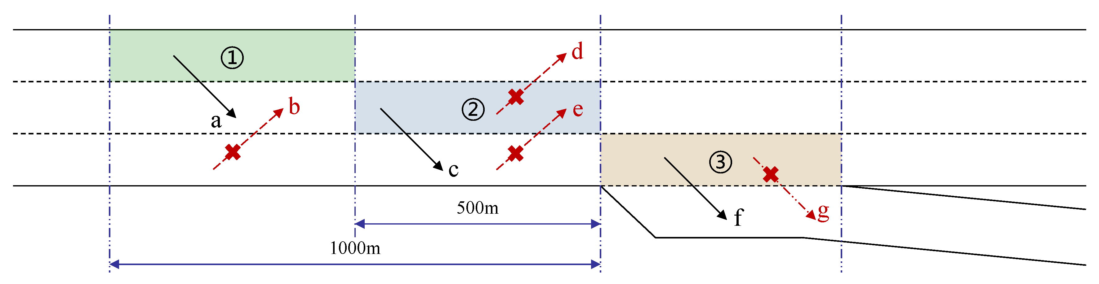According to the Chinese technical standard of highway engineering [39], ramps are generally positioned on the right side of the main road. Thus, MLC to the left arises as long as L3 SVs have to merge into the main road (usually the far-right lane) from the entrance ramp. Lane change to the right is not allowed for L3 SVs driving in the far-right lane within the merging area of the main road. In contrast, MLC to the right occurs when L3 SVs need to leave the main road (usually the far-right lane) from the exit ramp. In addition, to ensure that vehicles needing to exit can fully enter the far-right lane of the main road before entering the off-ramp diversion area, the distance from the off-ramp starting point to the vehicle will be used as a long-range perception input to L3 SVs and the lane control strategy relevant to the distance is applied to L3 SVs, as depicted in Figure 5 [40].

The area on the main road before the starting point of the diversion area is divided into three staggered regions, respectively ①, ②, and ③. Region ① filled with green color is set on the far-left lane of the main road. It starts from the position which is one kilometer away from the starting point of the diversion area and has a length of 500 m. Region ② filled with blue color is arranged in the middle lane of the main road. Its starting point is located at the endpoint of the first region while its endpoint is located at the starting point of the diversion area. Region ③ filled with grey color is disposed on the far-left lane of the main road with the same length as the diversion area. As for the L3 SVs, whose next road section on their path is the exit ramp, MLC to the right depicted by the black arrows a, c, and f in Figure 4 is necessary if they are running in all three regions. Moreover, they are not allowed to execute the lane change to the left as indicated by the red arrows b, d, and e in Figure 5. When the traffic flow rate is supersaturated, with high traffic density and small space headways between vehicles, implementing MLC becomes more challenging. If an L3 SV in a certain area fails to enter the designated lane, it will brake at a constant deceleration and eventually stop at the end of the area. During the deceleration period, MLC can be executed whenever the condition is suitable. In terms of the L3 SVs that continue driving on the main road and do not exit from the off-ramp, the lane change to the right is forbidden, which is marked as the red arrow g in Figure 5.

The priority of DLC lies between MLC and longitudinal driving behavior, which means that DLC may take place all the time except for the lane change behaviors prohibited in the aforementioned MLC. DLC for L3 SVs is controlled by model MOBIL, considering the overall benefit brought by the lane change to the local driving environment as a decision variable for the lane change [41]. If the overall benefit is larger than the threshold, the DLC demand appears. Otherwise, the subject vehicle maintains the longitudinal driving state. The overall benefit consists of three parts: the impacts of the subject vehicle’s lane change on the accelerations of itself and the following vehicles in the original lane, as well as the target lane. These acceleration impacts are defined as the differences between the accelerations in two scenarios: the DLC demand of the subject vehicle is satisfied or forbidden. Similar to the virtual accelerations in the safety judgment of a lane change, the accelerations under the assumption that the DLC demand is satisfied are calculated by IDM but the preceding vehicles for each vehicle are considered as the virtual leaders after DLC. The virtual leaders of the subject vehicle, the following vehicle of the subject vehicle in the same lane, and the following vehicle of the subject vehicle in the target lane, are the subject vehicle’s current leader in the target lane, the subject vehicle’s current leader the same lane, and the subject vehicle itself, respectively. The details of MOBIL can be obtained in [41].

When the midpoint of the front bumper of an L3 SV during a lane change reaches the centerline of the target lane, the vehicle is about to complete the lane change. It has to adjust its steering wheel to restore the vehicle’s travel direction to align with the lane guidance.

3.5.2. HVs’ Behavior Selection Models

MLC and DLC also exist in HVs. Both of them are controlled by the default model of VISSIM. The MLC model of HVs is much simpler than that of L3 SVs. Because of the lack of beyond-line-of-sight perception ability, an HV needing to enter the off-ramp cannot obtain its accurate distance to the start point of the diversion region. As a result, the lane control strategy in Figure 4 is not applicable and HVs planning to leave the main road may execute lane change anywhere before the endpoint of the diversion region. In the extreme scenario, if an HV needs to exit the highway and is still in the leftmost lane of the main road within the diversion area, it will stop before reaching the end of the merging area to wait for a gap to change lanes. Afterward, it will proceed to consecutively change three lanes to enter the exit ramp, which will probably cut down traffic flow on the main road and lead to or aggravate congestion. The extreme scenario may occur if drivers are unfamiliar with road conditions or when there is a traffic jam on the main road. As for DLC, HVs come up with the demand only based on the benefits to themselves in case the lane change has been completed. The impacts of the lane change on other surrounding vehicles are ignored except for the safety impact.

3.6. Chapter Summary

In order to develop the driving models for SVs, a two-dimensional general modeling architecture of SVs was built at the beginning of this section, based on which the intelligent driving behaviors of SVs with various intelligence levels were decomposed according to their typical application scenarios. Finally, returning to the theme of this study, the basic characteristics and capabilities, driving behavior models, and behavior selection models of L3 SVs and HVs were determined. The driving behavior and behavior selection models of the two kinds of vehicles are listed in

Table 4. The driving behavior and behavior selection models of L3 SVs and HVs.

Vehicle Type		Behavior Selection Model	Driving Behavior Model
			Longitudinal Model	Lateral Model
L3 SV	L3 AV	MLC: the lane control strategy DLC: MOBIL based on IDM	IDM	Safety judgment based on IDM
	L3 CAV		CIDM
HV		The default model of VISSIM based on Wiedemann 99	Wiedemann 99	Default model in VISSIM 2021

.

4. Traffic Impact Assessment

4.1. Traffic Impact Assessment Indicators

Traffic efficiency and energy consumption are the two dimensions of traffic impact evaluated in this research. Each dimension requires more specific indicators for explanation. The indicators on behalf of traffic efficiency were chosen based on the traffic theory. Traffic flow can be characterized by three basic parameters, which are traffic volume, average speed, and average density [37]. These three parameters are independent of each other, and the third parameter can be obtained if any two of them are known. Therefore, only two parameters of traffic flow are needed as the indexes due to the independence requirement. In addition, as the ultimate goal of this study was to obtain the economic benefits of L3 SVs’ traffic impacts, the convenience of economic quantification must be considered simultaneously. Consequently, the actual road capacity $Q_{xyz}$ [veh/h], reflecting the traffic volume, and the average travel time per vehicle per kilometer $T_{xyz}$ [s], transforming from the average speed, were confirmed as the evaluation indicators of traffic efficiency.

Traffic energy consumption is more intuitive than traffic efficiency because energy itself is a well-defined physical quantity. However, energy resource consumption is more common than energy consumption. Due to the fact that the power type of a vehicle was not the research variable in this research and that the trend of vehicle electrification is rapidly spreading, it was assumed that all simulated vehicles were battery-electric vehicles (BEVs). As a result, the electric average energy consumption per vehicle per kilometer ${EC}_{xyz}$ [kWh/km] was determined as the indicator of traffic energy consumption, which can be obtained by dividing the total energy consumption ${EC}_{xyz}^{sum}$ [kWh] by the total mileage ${\mathrm{V}\mathrm{M}\mathrm{T}}_{xyz}$ [kWh]. The Virginia tech comprehensive power-based electric vehicle energy consumption model (VT-CPEM) was used as the algorithm for ${EC}_{xyz}^{sum}$ [42]. It is an energy consumption model specially developed for BEVs. Electric energy consumption was calculated by reversing the traction force required by the wheels along the transmission chain, making it possible to take into account the instantaneous braking energy regeneration of BEVs. Moreover, VT-CPEM can be easily implemented in microscopic traffic simulation because its input variables are the current speed and acceleration of a vehicle. The meaning and value of $x$, $y$, and $z$ are described in Section 5.1.2 and the specific algorithm of VT-CPEM can be found in [42]. Moreover, Beijing was selected as a case city for traffic economic benefit analysis, which will be explained specifically in Section 6.2. In order to make the results conform to Beijing’s actual fleet features as much as possible, five different sets of vehicle data including mass $m$ [kg], the front area $A$ [m²], and the aerodynamic drag coefficient $C_D$ were used. They were obtained from the battery electric sedan with the highest market share in a specific vehicle segment (from A00 to C), as shown in

Table 5. The values of the parameter m, A, and C_D of the energy consumption model.

Parameter Value	Vehicle Segment
	A00	A0	A	B	C
$m$	1180	1340	1625	1825	2130
$A$	2.332	2.574	2.591	2.688	2.838
$C_D$	0.210	0.223	0.245	0.236	0.208

. ${EC}_{xyz}$ is eventually output as the average of five results derived from corresponding data configurations weighted by the market shares of the selected vehicles.

4.2. Economic Benefit Model

To facilitate the analysis of the comprehensive effectiveness of SVs, an economic benefit model of traffic impacts proposed by the authors before was applied [26]. As shown in Figure 6, the model was divided into three layers. The first layer is the traffic impacts of L3 SVs including travel time, actual road capacity, and energy consumption. The second layer is the fleet features, travel features, road topology, and energy price. It is decoupled from the first layer. The features have significant regional characteristics and there are obvious differences between different cities. The third layer represents the economic benefits output by the model.

The total economic benefits of L3 SVs $TB$ [billion yuan] consist of the traffic efficiency benefits $TEB$ [billion yuan] and the traffic energy saving benefits $\mathrm{E}\mathrm{E}\mathrm{B}$ [billion yuan]. The former benefits are made up of two parts, which are time-saving economic benefits $\mathrm{T}\mathrm{S}\mathrm{E}\mathrm{B}$ [billion yuan] and construction economic benefits $CEB$ [billion yuan]. $\mathrm{T}\mathrm{S}\mathrm{E}\mathrm{B}$ is generated by the variation of the travel time that can be transformed into economic value through the average time value per capita. $CEB$ derives from the variation of the actual road capacity. For example, a three-lane urban expressway is designed to serve 5607 vehicles hourly [43]. If all HVs are substituted by L3 SVs, maybe two lanes are sufficient, which means that the road can save the construction costs of one lane. $EEB$ is produced by the variation of the average energy consumption per vehicle per kilometer, reflecting the capability of L3 SVs to reduce the electricity demand. $TSEB$ and $EEB$ are all influenced by $CEB,$ providing that the change in actual road capacity will correspond to the change in travel demand. The algorithm of the economic benefit model can be found in [26]. Special attention should be paid that the traffic economic benefits are calculated under the premise of consistent travel demand. Thus, the additional traffic volume terms in the TSEB and EEB algorithms of the original model were removed.

5. Simulation Settings

5.1. Boundary Conditions

5.1.1. The Road Type

According to Section 1, the urban expressway was identified as the research road type because of its applicability to L3 SVs and its high traffic-carrying capacity. The geometric structure and attribute parameters of the urban expressways are different among different cities. It is difficult to build a model that can include all the actual features of urban expressways across the country. Therefore, a standard meta-model of the urban expressway was constructed as the simulation road scenario, as depicted in Figure 7. The model was strictly set in accordance with the standards of China’s “Urban Comprehensive Transportation System Planning” based on the assumption that the road in reality should comply with construction standards [43]. Consequently, not only the impact that irregular road construction may have on the simulation results was shielded, but also the authenticity and reference value of the research results were enhanced. The main road was approximately 5 km long and had three lanes, each of which had a width of 3.75 m. There was an entrance ramp and an exit ramp on the right side of the expressway. The entrance ramp with a length of 430 m was located 1400 m from the left starting point of the main road. Vehicles entering the main road from the entrance ramp would go through a four-lane merging area with a length of 200 m after leaving the entrance ramp. The exit ramp with a length of 480 m was situated 1400 m from the right end point of the main road. Vehicles leaving the main road from the exit ramp have to pass a four-lane diversion region with a length of 120 m before entering the exit ramp. The distance between the end of the merging region and the starting point of the diversion region was 1800 m, which was large enough to avoid the impact of two ramps being too close to the main road traffic flow. The speed limit of the main road and the ramps were 100 km/h and 60 km/h, respectively.

Vehicles entered the road network both from the left starting point of the main road (point ①) and entrance ramp (point ②) where the input traffic flow rates are $Q_1^i$ [veh/h] and $Q_2^i$ [veh/h], respectively. The input traffic flow rate of the whole road network $Q^i$ [veh/h] is the sum of $Q_1^i$ and $Q_2^i$. $Q_1^i$ is equal to 85% of $Q^i$, while $Q_2^i$ makes up 15% of $Q^i$. In order to simulate different operating states of the traffic flow, such as the free flow, congested flow, and forced flow, scenario analysis was conducted on $Q^i$, referring to various saturations of the traffic low, as shown in

Table 6. Scenario analysis on ${\mathrm{Q}}^i$.

$\mathbf{The}\mathbf{Value}\mathbf{of}{\mathbf{Q}}^{\mathit{i}}$	The Saturation of the Traffic Flow
4486	0.8${\mathrm{Q}}^s$
5607	${\mathrm{Q}}^s$
6728	1.2${\mathrm{Q}}^s$
7850	1.4${\mathrm{Q}}^s$

. $Q^s$ represents the saturated traffic flow rate, which equals 5607 veh/h [43].

As for the routes, vehicles input from the entrance ramp would keep running on the main road until the endpoint of the main road (point ④). In order to maintain the same traffic flow rate on the on-ramp and off-ramp, 18% of vehicle input from the starting point of the main road would leave the main road from the off-ramp (point ③).

5.1.2. The Traffic Composition

The traffic flow in this research was made up of the L3 SVs and HVs. In order to explore the influence of the scale of SVs on their traffic impacts, SVs’ proportion $P_{SV}$ was set from 0 to 100% with a gradient of 25%. Thus, the proportion of HVs $P_{HV}$ was equal to the value of $(1-P_{SV})$. Moreover, further analysis was conducted on the composition of SV’s fleet under certain SVs’ proportions. The share of CAVs among SVs $P_{CAV}$ varied from 0 to 100% while the ratio of AVs among SVs $P_{AV}$ was equal to the value of $(1-P_{CAV})$, increasing from 100% to 0. Both the decrease and increase gradients were 25%.

To make the traffic flow more closely resemble the real situation, on the one hand, HVs were differentiated in terms of driving styles. The driving style was divided into three types, which were aggressive style, neutral style, and conservative style. Their respective proportions to the total were 24.5%, 19.7%, and 55.8% [44,45]. On the other hand, the distracted driving behavior of human drivers was considered. According to relevant studies, it will occur with a probability of 15.3% at each simulation moment and last for 0.9 s [37,46,47,48,49]. These two values of distraction could be entered directly into VISSIM 2021.

In summary, various research scenarios were represented by $s_{xyz}$. $x$, $y$, and $z$ are the indexes on behalf of the input traffic flow rate, the proportion of L3 SVs, and the ratio of L3 CAVs, respectively, as shown in Table 6, There were 116 scenarios with different combinations of $x$, $y$, and $z$. When $y$ equals 0, there is no need to discuss different values of $z$ because the traffic flow at this time only consists of HVs, and $s_{x0z}$ under a certain value of $x$ is regarded as the baseline scenario.

5.2. Simulation Software and Its Technical Parameter

The simulation experiments of this study were completed by VISSIM 2021, which is one of the most common microscopic traffic simulation software in the world. It can not only conduct detailed modeling of key features of road sections and networks but also flexibly simulate the various driving behaviors of vehicles. The driving behavior of HVs was simulated using the default model of VISSIM 2021, while the driving behavior of SVs was implemented through a DLL file written in C++, which was linked to VISSIM 2021 with the help of the application program interface. The simulation experiment corresponding to each scenario was executed five times, and the relevant traffic impact indicators were averaged from the five experiments to reduce accidental errors. The random seed increment for each experiment was one to ensure that the five simulation experiments had different results. The duration of each simulation experiment was 1800 s, which could fully guarantee that the traffic flow in the experiment reached a stable input state.

6. Results

The letters A to E in Figure 8, Figure 9, Figure 10, Figure 11 and Figure 12 separately represent the proportion of CAVs among SVs, varying from 0 to 100% at a gradient of 25%. In the standard scenario, the traffic flow consisted only of human-driven vehicles. The value of travel time, actual road capacity, and energy consumption of each standard scenario is shown in the third row of Table 7, Table 8 and Table 9.

6.1. The Traffic Impacts of L3 SVs

6.1.1. The Impact of L3 SVs on Travel Time

The impact of L3 SVs on travel time is depicted in Figure 8 and the values of the impact of L3 SVs on travel time are listed in Table 7. Increasing the $P_{SV}$ can prominently shorten $T_{xyz}$. Under a certain $P_{CAV}$, the higher the $P_{SV}$, the more remarkable the time-saving effect. When $Q^i$ equaled 0.8 times $Q^s$, $Q^s$, 1.2 times $Q^s$, and 1.4 times $Q^s$, the maximum reduction of $T_{xyz}$ was 28.05%, 51.78%, 52.84%, and 38.12%, respectively. In terms of the impacts of SVs’ technology routes, when $Q^i{=0.8Q}^s$, raising the $P_{CAV}$ could further reduce travel time, but the degree of reduction was relatively small. When $Q^i{\ge 0.8Q}^s$, increasing the $P_{CAV}$ under the condition that $P_{SV}\le 25\%$ would cause fluctuations in travel time. When $P_{SV}\ge 50\%$, increasing the $P_{CAV}$ could further magnify the time-saving effect of SVs. The higher the $P_{SV}$, the more apparent the influence of increasing the $P_{CAV}$.

Figure 8. The impact of L3 SVs on travel time.

Figure 8. The impact of L3 SVs on travel time.

Table 7. The values of the Impacts of L3 SVs on travel time.

		Standard Scenario	${\mathit{P}}_{\mathit{S}\mathit{V}}$
${\mathit{Q}}^{\mathit{i}}$	${\mathit{P}}_{\mathit{C}\mathit{A}\mathit{V}}$		25%	50%	75%	100%
0.8$Q^s$	0	53.06 s	−19.60%	−24.70%	−25.72%	−26.10%
	25%		−20.84%	−24.05%	−26.04%	−26.36%
	50%		−20.18%	−24.91%	−26.06%	−26.89%
	75%		−21.62%	−24.85%	−26.63%	−27.48%
	100%		−21.55%	−25.03%	−26.94%	−28.05%
$Q^s$	0	81.09 s	−16.34%	−33.07%	−45.47%	−48.80%
	25%		−18.40%	−34.46%	−45.65%	−49.35%
	50%		−13.32%	−34.32%	−43.45%	−50.26%
	75%		−15.90%	−34.95%	−47.42%	−51.02%
	100%		−19.62%	−36.84%	−46.40%	−51.78%
1.2$Q^s$	0	88.66 s	−15.10%	−22.71%	−22.75%	−33.39%
	25%		−9.85%	−21.54%	−23.55%	−36.61%
	50%		−14.36%	−24.05%	−25.85%	−45.92%
	75%		−16.68%	−24.37%	−28.00%	−50.40%
	100%		−11.20%	−25.74%	−28.44%	−52.84%
1.4$Q^s$	0	92.33 s	−13.29%	−20.72%	−21.68%	−18.97%
	25%		−14.40%	−19.16%	−20.36%	−25.99%
	50%		−11.24%	−21.01%	−21.68%	−32.27%
	75%		−13.60%	−21.97%	−23.47%	−36.85%
	100%		−11.93%	−22.40%	−23.99%	−38.12%

Table 7. The values of the Impacts of L3 SVs on travel time.

		Standard Scenario	${\mathit{P}}_{\mathit{S}\mathit{V}}$
${\mathit{Q}}^{\mathit{i}}$	${\mathit{P}}_{\mathit{C}\mathit{A}\mathit{V}}$		25%	50%	75%	100%
0.8$Q^s$	0	53.06 s	−19.60%	−24.70%	−25.72%	−26.10%
	25%		−20.84%	−24.05%	−26.04%	−26.36%
	50%		−20.18%	−24.91%	−26.06%	−26.89%
	75%		−21.62%	−24.85%	−26.63%	−27.48%
	100%		−21.55%	−25.03%	−26.94%	−28.05%
$Q^s$	0	81.09 s	−16.34%	−33.07%	−45.47%	−48.80%
	25%		−18.40%	−34.46%	−45.65%	−49.35%
	50%		−13.32%	−34.32%	−43.45%	−50.26%
	75%		−15.90%	−34.95%	−47.42%	−51.02%
	100%		−19.62%	−36.84%	−46.40%	−51.78%
1.2$Q^s$	0	88.66 s	−15.10%	−22.71%	−22.75%	−33.39%
	25%		−9.85%	−21.54%	−23.55%	−36.61%
	50%		−14.36%	−24.05%	−25.85%	−45.92%
	75%		−16.68%	−24.37%	−28.00%	−50.40%
	100%		−11.20%	−25.74%	−28.44%	−52.84%
1.4$Q^s$	0	92.33 s	−13.29%	−20.72%	−21.68%	−18.97%
	25%		−14.40%	−19.16%	−20.36%	−25.99%
	50%		−11.24%	−21.01%	−21.68%	−32.27%
	75%		−13.60%	−21.97%	−23.47%	−36.85%
	100%		−11.93%	−22.40%	−23.99%	−38.12%

6.1.2. The Impact of L3 SVs on the Actual Road Capacity

The impact of L3 SVs on the actual road capacity under saturated and supersaturated traffic flow is shown in Figure 9, and the values of the impact of L3 SVs on the actual road capacity are listed in Table 8. When $Q^i{<Q}^s$, L3 SVs had no impact on $Q_{xyz}^r$ because the traffic flow operating state itself was in a free-flow state at this time. When $Q^i{=Q}^s$, $Q_{xyz}^r$ could be increased by up to 15.74% compared with the baseline scenario, and 0.92% compared with $Q^i$. When $P_{SV}\ge 50\mathrm{\%}$, continuing to increase the $P_{SV}$ exerted little influence on $Q_{xyz}$ because it had been close to or reached the theoretical upper limit. Under the same $P_{SV}$ that was smaller than 75%, increasing the $P_{CAV}$ could appropriately increase $Q_{xyz}$. As for the scenario that $Q^i{=1.2Q}^s$, $Q_{xyz}$ could be improved by up to 38.67% compared with the baseline scenario, and 0.39% compared with $Q^i$. Moreover, $Q_{xyz}$ could even be increased by up to 20.46% compared with $Q^s$, which means that the actual road capacity had far surpassed the design value of the road capacity. Under the same $P_{SV}$, that is, lower than 100%, increasing the $P_{CAV}$ could further increase $Q_{xyz}$. In terms of the scenario that $Q^i{=1.4Q}^s$, $Q_{xyz}$ could be raised by up to 48.46% compared with the baseline scenario, and 8.33% compared with $Q^i$. In addition, the maximum value of $Q_{xyz}$ reached 1.3 times $Q^s$, which also indicates that the actual road capacity far exceeded the design value of the road capacity. Under the same $P_{SV}$, that is, not larger than 50%, the improvement effect was not significant.

Figure 9. The impact of L3 SVs on the actual road capacity.

Figure 9. The impact of L3 SVs on the actual road capacity.

Table 8. The values of the impacts of L3 SVs on the actual road capacity.

		Standard Scenario	${\mathit{P}}_{\mathit{S}\mathit{V}}$
${\mathit{Q}}^{\mathit{i}}$	${\mathit{P}}_{\mathit{C}\mathit{A}\mathit{V}}$		25%	50%	75%	100%
$Q^s$	0	4889 veh/h	9.07%	14.56%	15.74%	15.74%
	25%		9.38%	14.92%	15.74%	15.74%
	50%		9.60%	14.90%	15.74%	15.74%
	75%		8.64%	15.00%	15.74%	15.74%
	100%		10.09%	15.09%	15.74%	15.74%
1.2$Q^s$	0	4870 veh/h	10.64%	17.30%	24.26%	37.74%
	25%		10.53%	18.35%	25.71%	38.36%
	50%		10.81%	19.28%	27.64%	38.60%
	75%		11.14%	20.34%	29.41%	38.65%
	100%		11.12%	21.43%	31.18%	38.67%
1.4$Q^s$	0	4930 veh/h	9.90%	17.82%	24.35%	41.51%
	25%		9.95%	17.05%	24.08%	44.29%
	50%		10.43%	19.04%	26.95%	47.76%
	75%		11.87%	19.71%	28.68%	48.46%
	100%		11.33%	20.09%	29.90%	47.85%

Table 8. The values of the impacts of L3 SVs on the actual road capacity.

		Standard Scenario	${\mathit{P}}_{\mathit{S}\mathit{V}}$
${\mathit{Q}}^{\mathit{i}}$	${\mathit{P}}_{\mathit{C}\mathit{A}\mathit{V}}$		25%	50%	75%	100%
$Q^s$	0	4889 veh/h	9.07%	14.56%	15.74%	15.74%
	25%		9.38%	14.92%	15.74%	15.74%
	50%		9.60%	14.90%	15.74%	15.74%
	75%		8.64%	15.00%	15.74%	15.74%
	100%		10.09%	15.09%	15.74%	15.74%
1.2$Q^s$	0	4870 veh/h	10.64%	17.30%	24.26%	37.74%
	25%		10.53%	18.35%	25.71%	38.36%
	50%		10.81%	19.28%	27.64%	38.60%
	75%		11.14%	20.34%	29.41%	38.65%
	100%		11.12%	21.43%	31.18%	38.67%
1.4$Q^s$	0	4930 veh/h	9.90%	17.82%	24.35%	41.51%
	25%		9.95%	17.05%	24.08%	44.29%
	50%		10.43%	19.04%	26.95%	47.76%
	75%		11.87%	19.71%	28.68%	48.46%
	100%		11.33%	20.09%	29.90%	47.85%

6.1.3. The Impact of L3 SVs on Traffic Energy Consumption

The impact of L3 SVs on traffic energy consumption is shown in Figure 10. Increasing the $P_{SV}$ could apparently reduce ${EC}_{xyz}$. The values of the impact of L3 SVs on energy consumption are listed in Table 9. Under a fixed $P_{CAV}$, the higher the $P_{SV}$, the more significant the energy-saving effect. When $Q^i$ equals 0.8 times $Q^s$, $Q^s$, 1.2 times $Q^s$, and 1.4 times $Q^s$, the maximum reduction of ${EC}_{xyz}$ could be 7.28%, 18.72%, 27.44%, and 28.74%, respectively. As for the composition of L3 SVs, under the scenario that $Q^i{=0.8Q}^s$, increasing the $P_{CAV}$ did not have a significant impact on ${EC}_{xyz}$ when $P_{SV}<50\%$, but weakened the energy-saving effect as long as $P_{SV}\ge 50\%$. This is because CAV will increase the average speed of traffic flow under the free-flow state. A similar phenomenon was observed in the scenario where $Q^i{=Q}^s$. When $Q^i{=1.2Q}^s$ and $Q^i{=1.4Q}^s$, raising the $P_{CAV}$ under a certain $P_{SV}$ could further amplify the energy-saving effect of L3 SVs. However, when $Q^i{=1.2Q}^s$, continuing to increase the $P_{CAV}$ when the $P_{SV}$ and $P_{CAV}$ are equal to 100% and 50%, respectively, has almost no impact on the energy-saving effect of SV transportation because the traffic flow has already been in the free-flow state. When $Q^i{=1.4Q}^s$, continuing to increase the $P_{CAV}$ when the $P_{SV}$ and $P_{CAV}$ are equal to 100% and 25% will weaken the energy-saving benefits for the reason that the average traffic speed is improved.

Figure 10. The impact of L3 SVs on traffic energy consumption.

Figure 10. The impact of L3 SVs on traffic energy consumption.

Table 9. The values of the impacts of L3 SVs on energy consumption.

		Standard Scenario	${\mathit{P}}_{\mathit{S}\mathit{V}}$
${\mathit{Q}}^{\mathit{i}}$	${\mathit{P}}_{\mathit{C}\mathit{A}\mathit{V}}$		25%	50%	75%	100%
0.8$Q^s$	0	0.63 kWh/km	−1.42%	−3.22%	−5.42%	−7.28%
	25%		−1.24%	−3.02%	−5.41%	−7.27%
	50%		−1.08%	−3.24%	−5.30%	−6.97%
	75%		−1.43%	−3.38%	−5.14%	−6.59%
	100%		−1.34%	−3.31%	−4.96%	−6.06%
$Q^s$	0	0.179 kWh/km	−9.22%	−14.60%	−16.09%	−18.72%
	25%		−7.99%	−14.51%	−16.53%	−18.34%
	50%		−10.62%	−14.92%	−16.50%	−17.88%
	75%		−8.80%	−14.92%	−15.66%	−17.11%
	100%		−10.27%	−14.69%	−15.49%	−16.28%
1.2$Q^s$	0	0.186 kWh/km	−6.17%	−13.10%	−15.07%	−24.14%
	25%		−7.08%	−15.73%	−15.88%	−25.40%
	50%		−6.30%	−15.14%	−16.95%	−27.30%
	75%		−7.30%	−15.40%	−17.24%	−27.44%
	100%		−7.10%	−17.44%	−17.97%	−27.09%
1.4$Q^s$	0	0.190 kWh/km	−5.44%	−13.00%	−15.05%	−28.22%
	25%		−6.08%	−12.80%	−15.33%	−30.20%
	50%		−6.24%	−14.50%	−15.88%	−29.61%
	75%		−4.79%	−13.99%	−15.96%	−28.09%
	100%		−6.09%	−15.37%	−16.10%	−26.30%

Table 9. The values of the impacts of L3 SVs on energy consumption.

		Standard Scenario	${\mathit{P}}_{\mathit{S}\mathit{V}}$
${\mathit{Q}}^{\mathit{i}}$	${\mathit{P}}_{\mathit{C}\mathit{A}\mathit{V}}$		25%	50%	75%	100%
0.8$Q^s$	0	0.63 kWh/km	−1.42%	−3.22%	−5.42%	−7.28%
	25%		−1.24%	−3.02%	−5.41%	−7.27%
	50%		−1.08%	−3.24%	−5.30%	−6.97%
	75%		−1.43%	−3.38%	−5.14%	−6.59%
	100%		−1.34%	−3.31%	−4.96%	−6.06%
$Q^s$	0	0.179 kWh/km	−9.22%	−14.60%	−16.09%	−18.72%
	25%		−7.99%	−14.51%	−16.53%	−18.34%
	50%		−10.62%	−14.92%	−16.50%	−17.88%
	75%		−8.80%	−14.92%	−15.66%	−17.11%
	100%		−10.27%	−14.69%	−15.49%	−16.28%
1.2$Q^s$	0	0.186 kWh/km	−6.17%	−13.10%	−15.07%	−24.14%
	25%		−7.08%	−15.73%	−15.88%	−25.40%
	50%		−6.30%	−15.14%	−16.95%	−27.30%
	75%		−7.30%	−15.40%	−17.24%	−27.44%
	100%		−7.10%	−17.44%	−17.97%	−27.09%
1.4$Q^s$	0	0.190 kWh/km	−5.44%	−13.00%	−15.05%	−28.22%
	25%		−6.08%	−12.80%	−15.33%	−30.20%
	50%		−6.24%	−14.50%	−15.88%	−29.61%
	75%		−4.79%	−13.99%	−15.96%	−28.09%
	100%		−6.09%	−15.37%	−16.10%	−26.30%

6.2. The Economic Benefits of L3 SVs’ Traffic Impacts

This study used Beijing’s peak hours as a case. The travel and road network conditions, and energy price shown in

Table 10. The travel and road network conditions, as well as the energy price in Beijing.

Feature	Parameter	Unit	Value
Travel structure	Number of people traveling by passenger cars in the central city on weekdays	Person-time	8,120,000
	Proportion of passenger car trips during peak hours to full-day passenger car trips	-	30.3%
	Average one-way commute distance during weekday peak hours	km	13.89
	Usage intensity ratio of urban expressways during peak hours on weekdays	-	66.52%
	Number of private passenger cars	veh	4,940,000
	Vehicle usage rate on weekdays	time	77.0%
Road network structure	Total mileage of urban expressways	km	780
	Average traffic saturation of urban expressways during peak periods	-	1.2
Energy price	Average charging costs for BEV	CNY/kWh	0.722

, as well as the traffic efficiency and energy consumption impact results of L3 SVs, were input into the economic benefit model to calculate the traffic economic benefits of L3 SVs [50,51,52,53]. Beijing has a good policy environment for the development of SVs. It encourages pilot application projects for SVs and has established SV policy pilot areas and multiple test roads for intelligent driving. Therefore, L3 SVs may be popularized first and quickly in Beijing. Beijing’s road types are representative nationwide. It has several urban expressways around the city and radiating from the city center [50]. Such a road network structure is one of the typical representatives of China’s urban expressway topology, providing a suitable road network environment for L3 SVs. In addition, there is excessive traffic demand during peak hours in Beijing [50]. The traffic demand in rush hours on Beijing’s urban expressways exceeds the design capacity of the roads, and some roads are even congested throughout the day, corresponding to the area where the traffic optimization effect of L3 SVs is prominent. Consequently, according to the traffic impact results, once L3 SVs are applied, a positive influence on traffic efficiency and energy consumption, as well as considerable economic benefits, will take place. The usage intensity ratio of urban expressways during peak hours on weekdays is hard to obtain directly, whose calculation method can be found in [26].

SVs can contribute to significant traffic economic benefits, as depicted in Figure 11. The benefits gradually increase as the input traffic flow rate changes from an unsaturated state to a supersaturated state but will fall back when $Q^i{\gg Q}^s$. When $Q^i{<Q}^s$, if the $P_{SV}$ exceeds 50% and continues to increase, the impacts of the $P_{SV}$ and $P_{CAV}$ on traffic economic benefits are not significant. When $Q^i{\ge Q}^s$, the improvement of the $P_{SV}$ and $P_{CAV}$ can further improve the economic benefits of transportation remarkably. The values of L3 SVs’ traffic economic benefits are listed in

Table 11. The values of L3 SVs’ traffic economic benefits.

		${\mathit{P}}_{\mathit{S}\mathit{V}}$
${\mathit{Q}}^{\mathit{i}}$	${\mathit{P}}_{\mathit{C}\mathit{A}\mathit{V}}$	25%	50%	75%	100%
0.8$Q^s$	0	0.414	0.536	0.579	0.606
	25%	0.437	0.521	0.391	0.611
	50%	0.422	0.540	0.543	0.619
	75%	0.455	0.541	0.620	0.627
	100%	0.452	0.543	0.432	0.633
$Q^s$	0	0.846	1.568	2.001	2.135
	25%	0.904	1.619	2.012	2.147
	50%	0.781	1.619	1.943	2.170
	75%	0.816	1.641	2.057	2.185
	100%	0.986	1.700	2.023	2.200
1.2$Q^s$	0	0.858	1.368	1.571	2.384
	25%	0.687	1.387	1.644	2.524
	50%	0.839	1.489	1.785	2.869
	75%	0.938	1.530	1.906	3.024
	100%	0.749	1.628	1.975	3.104
1.4$Q^s$	0	0.792	1.646	1.578	2.084
	25%	0.840	1.667	1.528	2.429
	50%	0.743	1.735	1.656	2.734
	75%	0.846	1.765	1.765	2.896
	100%	0.789	1.850	1.816	2.903

. The maximum benefit is CNY 0.633, 2.200, 3.104, and 2.903 billion yuan when the input traffic flow rate reaches four-fifths, 1 time, 1.2 times, and 1.4 times the saturated traffic flow rate, respectively.

Figure 11. Theeconomic benefits of Beijing from the traffic impacts of L3 SVs.

Figure 11. Theeconomic benefits of Beijing from the traffic impacts of L3 SVs.

Among the three different types of economic benefits that constitute the total economic benefits, $TSEB$ accounted for the highest proportion while $EEB$ made up the lowest proportion, as shown in Figure 12. When $Q^i{<Q}^s$, no matter how $P_{SV}$ changed, the traffic flow was always in a free-flow state, and the $CEB$ was always 0. When $Q^i{\ge Q}^s$, the traffic flow was in a congested-flow or even forced-flow state. SVs can bring a significant $CEB$, and the higher the degree of supersaturation of the $Q^i$, the more prominent the $CEB$.

Figure 12. The structure of L3 SVs’ traffic economic benefits.

Figure 12. The structure of L3 SVs’ traffic economic benefits.

7. Conclusions and Discussion

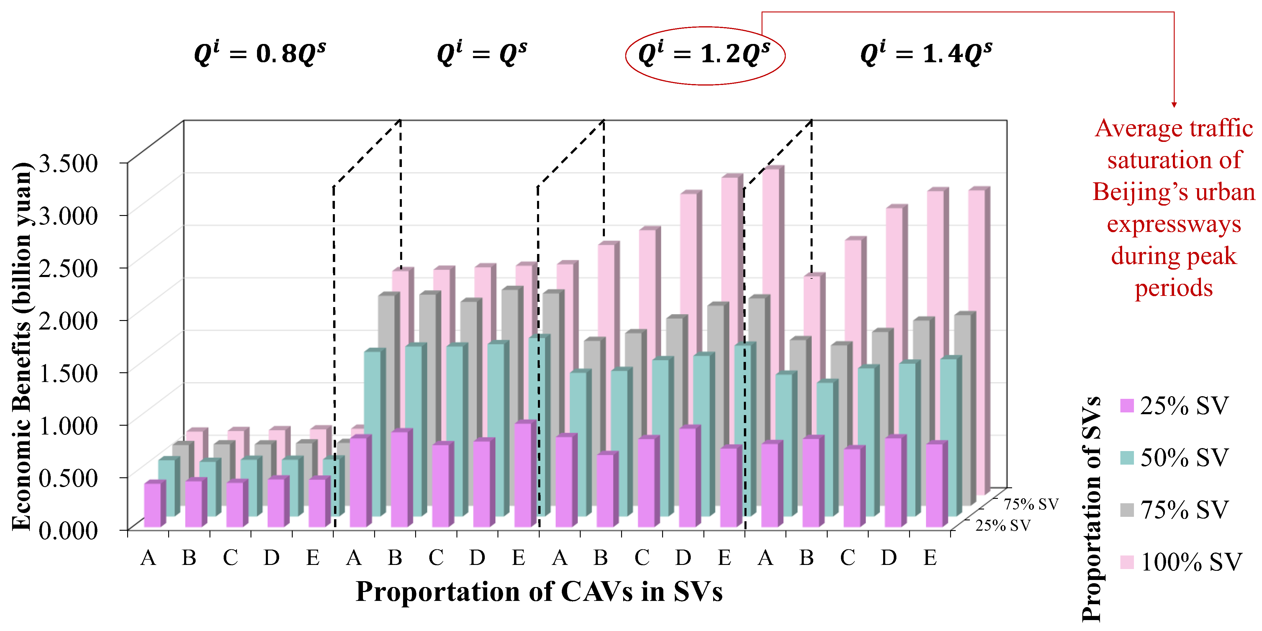
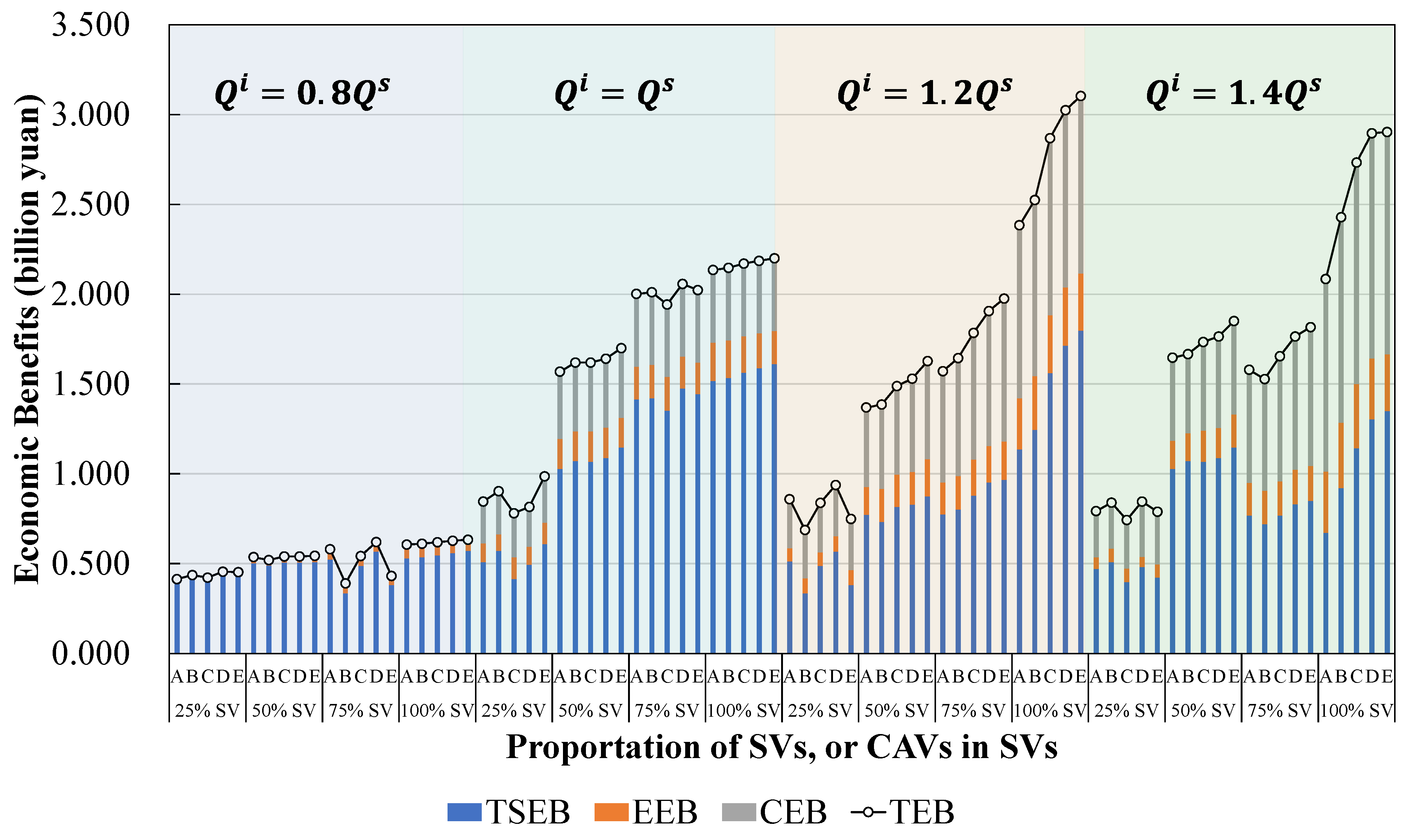
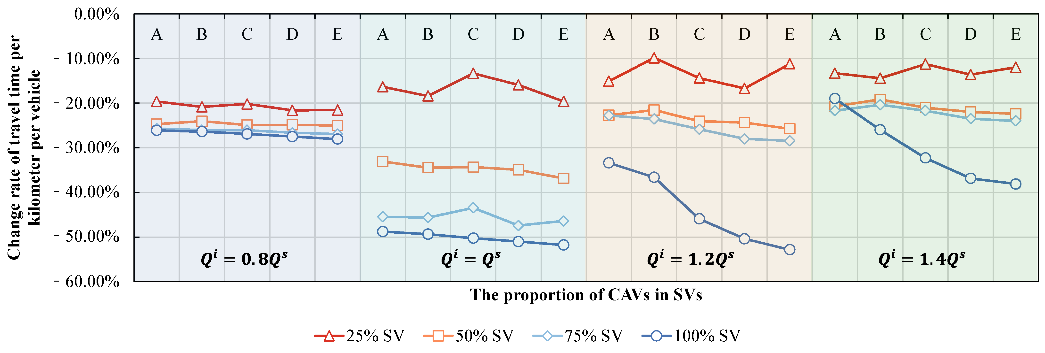
This study conducted an assessment of the L3 SVs’ impacts on traffic efficiency and energy consumption based on a microscopic traffic simulation. Not only were the traffic impacts analyzed, but the corresponding economic benefits were also calculated. The research roadmap was proposed at the very beginning as the guideline, clarifying the input, output, and core modules. Next, a general framework for the evaluation of SVs’ traffic impacts was established, identifying the variables and boundary conditions. As for the variables, it is of great importance to build the driving models for SVs with different intelligent driving levels. A two-dimensional general modeling architecture for SVs was proposed. Based on the architecture, the intelligent driving behavior of SVs with various intelligent driving levels was decomposed into three layers, which were vehicle capability, driving behaviors, and behavior selection. Three crucial elements that are applicable road types, intelligent decision-making logic, as well as intelligent configuration, were integrated simultaneously according to the decomposition results. L3 SVs’ driving models were eventually constructed on the basis of the architecture. The boundary conditions were made up of the road type and traffic conditions. The urban expressways were selected as the road type and complex traffic conditions including the input traffic flow rate, and the proportions of SVs and CAVs were taken into account. It was found that L3 SVs could exert remarkable effects on traffic efficiency and energy consumption. The impact on travel time was more significant when the input traffic flow rate was around the saturated traffic flow rate. The average travel time per kilometer could be reduced by 19.60–28.05%, 7.99–51.78%, 9.85–52.84%, and 11.24–38.12% compared to the standard scenario that the traffic flow is just made up of HVs when the input traffic flow rate equals 0.8 times, 1 time, 1.2 times, and 1.4 times of the saturated traffic flow rate, respectively. The influence on the actual road capacity would appear only if the input traffic flow rate reaches or exceeds the saturated value, where the traffic flow will change from a free-flow state to a congested or even forced state. The actual road capacity would increase by 9.07–15.74%, 10.53–38.67%, and 9.90–48.46% compared to the standard scenario when the input traffic flow rate is equal to 1 time, 1.2 times, and 1.4 times the saturated traffic flow rate, respectively. Furthermore, L3 SVs showed good performance in traffic energy saving. Energy consumption would decrease by 1.08–7.28%, 7.99–18.72%, 6.17–27.44%, and 4.79–28.74% compared to the standard scenario when the input traffic flow rate reaches four-fifths, 1 time, 1.2 times, and 1.4 times of the saturated traffic flow rate, respectively. It should be noted that the intervals are caused by differences in traffic flow composition. The right endpoints of the intervals often occur when the proportion of SVs reaches 100% and the proportion of CAVs is high. The special cases exist in the impacts on traffic energy consumption because the greater average speed of traffic flow caused by a high proportion of CAVs may raise energy consumption, leading to a negative effect on traffic energy saving.

According to the results of L3 SVs’ traffic impacts, the relevant economic benefits were obtained based on Beijing’s real traffic and fleet conditions during peak hours. The maximum benefits could be CNY 0.633, 2.200, 3.104, and 2.903 billion when the input traffic flow rate reaches four-fifths, 1 time, 1.2 times, and 1.4 times the saturated traffic flow rate, respectively. All of them occurred when the proportions of L3 SVs and L3 CAVs were both 100%.

In order to give full play to the role of L3 SVs in improving traffic efficiency and saving traffic energy consumption, and fully realize related traffic benefits, L3 SVs’ proportion should be promoted as soon as possible. Although the Chinese government has promulgated policies to promote the demonstration pilot of L3 SVs application, there are still many obstacles remaining to be cleared such as technology maturity, the division of responsibility for accidents, and business models. The government should increase the support for L3 SVs in terms of policy, law, and finance to improve their market penetration. Moreover, the government should also speed up the improvement of the coverage density of intelligent transportation infrastructures. It is claimed that CAVs perform better than AVs in improving actual road capacity and saving travel time as well as energy, contributing to higher traffic economic benefits. Thus, on the one hand, intelligent transportation infrastructures can enable intelligent driving based on V2I, with the help of which AVs are able to upgrade to CAVs so that the higher benefits would be realized. On the other hand, intelligent transportation infrastructure can share the costs of SV deployment by sharing the technical requirements of the vehicle, thus reducing the price of L3 SVs. The cheaper the L3 SVs, the higher their penetration rate and proportion. OEMs must closely adhere to the product attributes of L3 SVs, and anchor relatively simple and easy scenarios to promote their rapid implementation so that consumers can truly appreciate the optimization of driving experience by L3 SVs. The road type in this study, urban expressways, is very suitable for the first application of L3 SVs. First, they are fully closed roads and the traffic environment is relatively simple. As a result, there is less challenge on urban expressways and the probability of long-tail scenarios that render the intelligent driving system ineffective is relatively low. Second, high-precision maps have already covered the urban expressways in most first- and second-tier domestic cities, providing complete technical support for L3 SVs. Third, urban expressways bear the largest traffic volume with the shortest distance in the urban road network. Their traffic flow rate during peak hours is usually beyond the saturated value so that the traffic efficiency and energy-saving reduction benefits of L3 SV can be fully realized.

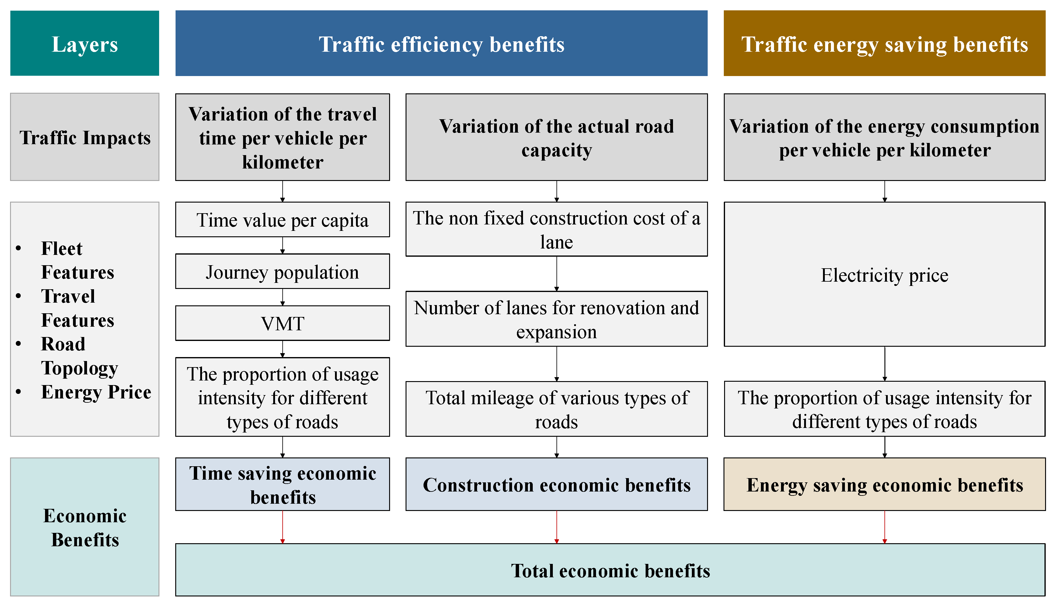
This study provides a paradigm for the evaluation of the traffic impacts from SVs. Some changes will be necessary if it is applied to other districts. The fleet features, travel features, road topology, and energy prices of the economic benefit model should be modified to stay consistent with the real situation of the cities. The traffic impact results of SVs are common between different cities in the same country because the road in the simulation was modeled according to national standards. However, the results of traffic influences from SVs should be changed if the study is going to be conducted in cities or towns in different countries. This is because the construction standards for a certain type of road, the application scenarios of SVs, and the driving behavior of human drivers vary among countries.

This study still has some shortcomings, which will be improved in subsequent research. First, all vehicles in this study are BEVs but the vast majority of vehicles in the current fleet are gasoline-powered vehicles. In order to improve the accuracy of the economic benefit results, the power composition of the fleet will be further refined. Second, the traffic situation in China is complex, such that the driving behavior of different kinds of human drivers may not always remain constant. Therefore, in the future, the model parameters will be carefully calibrated and verified according to different traffic scenarios. Third, the simulation experiments were conducted under relatively ideal urban expressway scenarios in China, which may lead to an underestimation of SVs’ traffic benefits. In subsequent research, the roadmap of China’s cities will be further refined to enhance the authenticity and reliability of the research results. Fourth, the boundary conditions in this study mainly focused on road traffic, like the road type and input traffic flow rate. It is meaningful to reveal the influence mechanism of more boundary conditions like weather and transportation infrastructure quality, which will help to better explain the traffic optimization mechanism of SVs. Fifth, the costs of L3 SVs were not considered. In the follow-up research, the net traffic economic benefits of SVs will be calculated based on their costs, and then a comprehensive cost-effectiveness analysis of SVs on different technical routes will be conducted.