Exploring the Effects of Socioeconomic Factors and Urban Forms on CO₂ Emissions in Shrinking and Growing Cities

Abstract

Exploring the mechanisms influencing carbon dioxide (CO₂) emissions is crucial to seeking low-carbon development paths. Previous studies have analyzed the effects of socioeconomic factors and urban forms on CO₂ emissions. However, little attention has been paid to the heterogeneity of their interactions in differing urban development patterns, such as growth and shrinkage. This study focused on how socioeconomic factors and urban forms work together to comprehensively affect CO₂ emissions within the context of urban shrinkage and growth. A selection of 285 prefecture-level cities in China were divided into four groups of shrinking and growing cities based on a comprehensive index system. After assessing variables involving socioeconomic factors and urban forms, a panel data model was used to verify their mutual mechanisms influencing CO₂ emissions. The results show that CO₂ emissions in shrinking cities continue to rise due to the driving force of secondary industry and the coexistence of population loss and space expansion. For growing cities, in addition to economic development and population growth, urban forms with excessive compactness and polycentricity significantly accelerate CO₂ emissions. Consequently, disorderly urban expansion should be avoided, and industrial upgrading should be promoted for shrinking cities. Meanwhile, growing cities are advised to develop modern service industries. Moreover, it is recommended that urban spatial planning follows urban functions and their development stages to avoid excessive agglomeration and polycentricity.

1. Introduction

Global warming is a major threat to environmental and human health and can result in serious consequences, such as rising sea levels, glacier melting, and extreme weather events [1,2,3]. The most significant cause of this phenomenon is the increase in greenhouse gases (e.g., CO₂) released by burning fossil fuels [4,5]. Cities emit large amounts of CO₂ from activities such as engineering construction, industrial production, and transportation since they are regions where economic and social activities are concentrated. Besides, while cities account for only 3% of the world’s surface, they are the source of 78% of global CO₂ emissions [6,7]. However, with societal development and population growth, cities will likely continue consuming high amounts of energy and emitting CO₂ to support human life demands. Therefore, reducing urban CO₂ emissions is crucial to addressing the adverse effects of global warming.

Several authors suggest lowering urban CO₂ emissions through the control of socioeconomic variables such as population growth, industrial output, technology, and transportation [8,9,10,11,12]. Therefore, economic development and population expansion are expected to accelerate energy consumption, increasing carbon emissions. For instance, Sheinbaum et al. [13] reported that economic growth contributed 133.6% to the increase in CO₂ emissions from 1970 to 2006. Likewise, based on multivariate regression models, Muñiz et al. [14] reported that population growth promotes carbon emissions. However, socioeconomic development and CO₂ emissions do not always have a linear relationship [15,16]. For example, Iwata et al. [17] confirmed that an inverted U-shaped curve exists between economic growth and CO₂ emissions, consistent with the environmental Kuznets curve. Meanwhile, several studies have reported that CO₂ emissions may rise again when the economy of a given region exceeds a certain level [18,19]. In addition, Casey et al. [20] pointed out that the improvement in the population urbanization level at the regional scale will lead to the progress of technology, changes in the living patterns of residents, and the scale of public services, which may reduce regional CO₂ emissions. Therefore, the effects of socioeconomic factors on CO₂ emissions need to be explored in accordance with the specific conditions of cities.

In addition to socioeconomic factors, several researchers have explored the spatial link between urban forms and CO₂ emissions. Urban forms reflect the spatial organizational structure of urban landscapes, such as transportation, infrastructure, and functional areas. They regulate urban growth and expansion through the allocation of human and material resources and the impact of transportation structure and infrastructure layouts, thus profoundly affecting CO₂ emissions. Recent studies have reported that an increase in urban area, urban fragmentation, and urban irregularity accelerate urban CO₂ emissions, whereas compact urban forms reduce CO₂ emissions [21,22,23]. Shi et al. [24] reported that the expansion of urban areas aggravates CO₂ emissions significantly. Yi et al. [25] argued that compact urban forms reduced CO₂ emissions, although urbanization aggravates CO₂ emissions. However, Zuo et al. [26] proposed that carbon emissions in industrial and mixed-function zones would decrease with increasing regional fragmentation, but carbon emissions in public service, residential, and administrative regions would increase with increasing regional fragmentation. Regarding urban polycentricity, urban single-center developments may result in higher CO₂ emissions, and urban multi-center developments tend to lower CO₂ emissions [21,27,28]. However, contrasting views show that urban single-center developments with high density and compact urban form reduce CO2 emissions, mainly because of reduced transportation demands, shortened commuting distances, reduced infrastructure construction, and protected green space outside of the city [23,29]. Few studies have fully taken into account the variety of the geographical associations between urban forms and CO₂ emissions, especially in scenarios of urban shrinkage and growth.

In economic globalization, urban development paths describe two differing spatial phenomena: urban growth and shrinkage. The increasing differentiation between growth and shrinkage has been a nonnegligible form of urban development since the Industrial Revolution [27,30]. Urban shrinkage is often associated with economic downturns, which implies the deterioration of the social environment [31,32]. Sun et al. [33] reported that shrinking cities have lower eco-efficiency than growing cities, while Xiao et al. [34] reported that CO₂ emissions continued to rise in rapidly shrinking cities, although they peaked in other cities in China during 2011–2013. Tong et al. [35] indicated that the population and economy significantly promote carbon emissions, while in shrinking cities, technology and tertiary industries have significant negative effects on carbon emissions. Previous studies have shown that CO₂ emissions display differing patterns in growing and shrinking cities; however, urban forms have been neglected in most cases. Besides, most studies use population index as the main criterion for evaluating urban growth or shrinkage, but they have ignored that urban development is a multifaceted process. The multifaceted implications of urban growth and shrinkage cannot be adequately captured by a single population index.

Three research gaps are highlighted in the previous studies. Firstly, the relationship between urban forms, socioeconomic factors, and CO₂ emissions is still up for debate, and various conclusions are frequently drawn for various kinds of cities. Secondly, most studies have ignored that urban development is a multifaceted process and only used a single population index to divide growing and shrinking cities. Thirdly, the majority of current studies have ignored the fact that the influencing mechanism of urban carbon emissions is a comprehensive system including social, economic, and spatial systems.

China has made a commitment to actively reducing carbon emissions [36,37]. Nonetheless, the urban spatial form is ever-changing due to China’s rapidly increasing urbanization. As a result, regional development faces huge imbalances; moreover, population growth and shrinkage occur simultaneously [38,39,40]. Growing cities often face population inflow, economic growth, and industrial agglomeration. In contrast, shrinking cities face social and economic problems such as population loss, economic decline, industrial structure imbalance, and environmental degradation. The contrasting characteristics of shrinking and growing cities differentially affect CO₂ emissions [31,41,42]. Therefore, to achieve dual carbon goals in China, the following questions must be addressed: (1) how do socioeconomic factors and urban forms affect CO₂ emissions between growing and shrinking cities in China? (2) What are the suggestions for reducing CO₂ emissions under different development scenarios of urban growth and shrinkage?

Accordingly, our study explores how socioeconomic factors and urban forms interrelate to impact CO₂ emissions in shrinking and growing cities for supporting emission-reduction policy-making. A comprehensive index system was first constructed to divide growing and shrinking cities, and the effects of social economy and spatial structure on CO₂ emissions were explored by considering differing urban growing and shrinking scenarios. In addition, our study provides support for decision-making regarding sustainable development against the background of urban growth and shrinkage in China.

2. Materials and Methods

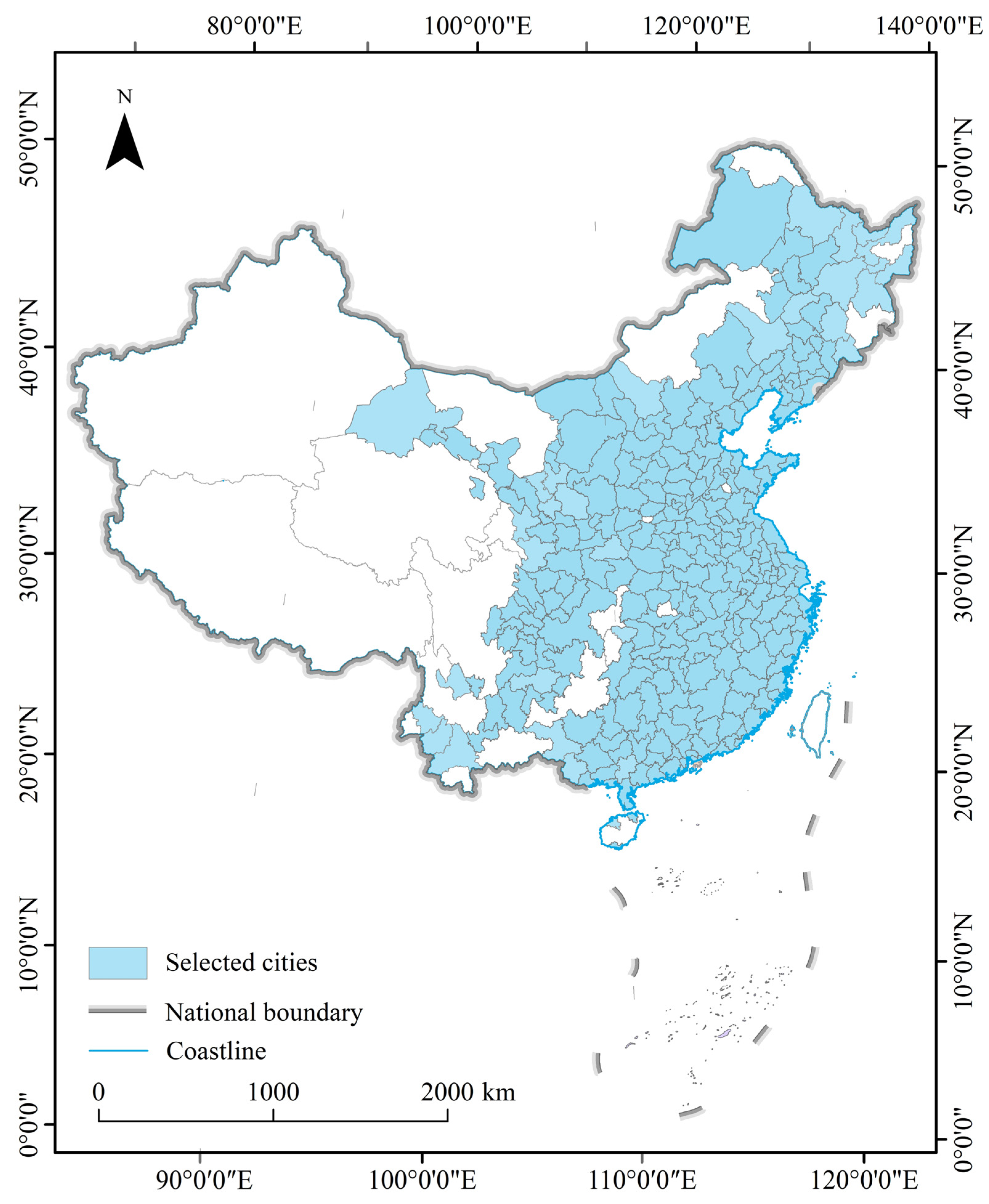
2.1. Study Area

Over the past decade, China has experienced urban growth and urban shrinkage, facing the double pressure of economic development and carbon reduction [43]. Such a situation in Chinese cities provides an excellent experimental subject for the patterns of CO₂ emissions in growing and shrinking cities. Considering the availability of statistical data, 285 cities (including 4 municipalities: Beijing, Tianjing, Shanghai, and Chongqing) were selected as experimental objects with reference to the definition of prefecture-level cities by Long et al. [44] (Figure 1). With a combined population of 1.21 billion, these cities make up around 93% of mainland China’s total population, according to the 2020 National Population Census. The selected cities are widely distributed and provided varied urban growth or urban shrinkage between 2005 and 2020, providing an ample perspective for exploring the patterns of CO₂ emission reduction under the contexts of urban growth and shrinkage.

2.2. Data Sources

Four types of data were collected and processed, including city-scale CO₂ emissions, urban boundary data, gridded population distribution data, and socioeconomic statistics. The details are as follows:

City-scale CO₂ emissions data from 2005– to 2020 were acquired from the China City Greenhouse Gas Working Group (CCG) [45]. The data were collected and verified by first-hand on-site data using a bottom-up method, resulting in high accuracy. CO₂ emissions were derived from China’s high-resolution geographic emissions grid data.

Urban boundary data (2005, 2010, 2015, and 2020) were used to quantify the indicators representing urban forms [46,47]. With a worldwide 10 m-resolution impervious surface, the data products were generated, and the accuracy was greater than 88.00%.

Gridded population distribution data were obtained from LandScan™ high-resolution global population data (https://www.satpalda.com/product/landscan/ (accessed on 12 May 2022)). The Landscan dataset estimates global population distributions with a density of approximately 1 km-by-1 km scale, and was used to quantify urban polycentricity.

Socioeconomic statistics were collected from the the China City Statistical Yearbook, including the following four indices: total population in the urban area (POP), gross domestic product (GDP), proportion of secondary industry (PSI), and proportion of tertiary industry (PTI).

2.3. Methods

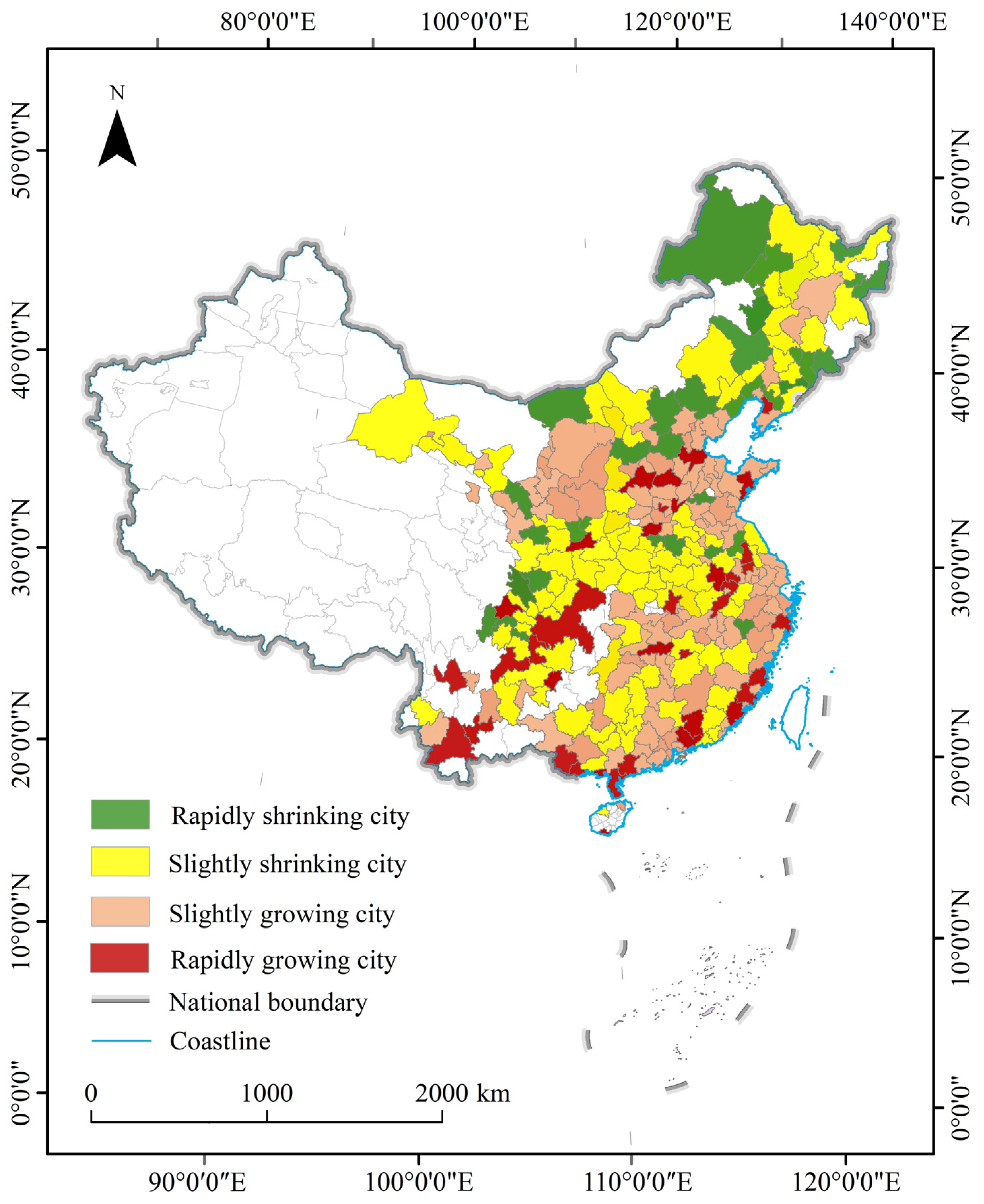
2.3.1. Classification of Growing and Shrinking Cities

Urban growth or shrinkage is a comprehensive concept that is based on population increase or decrease and reflects the development problems such as land use efficiency, public infrastructure, economic development, fiscal revenue, and social public service capacity [48,49]. Referring to Tong et al. [35], this study focused on four dimensions—population, economy, space, and society—in order to build a multidimensional evaluation system for urban growth and shrinkage (

Table 1. Identification system for urban growth and shrinkage [35].

Dimensions	Indicators	Unit
Population	Natural population growth rate	%
	Total population	104 Person
	Population density	Person/km2
Economic	Per capita GDP	Yuan
	Per capita fiscal revenue	Person/Yuan
	GDP growth rate	%
Space	The urban expansion rate	%
	Built-up area	Km2
Society	Total retail sales of consumer goods	104 Yuan
	Per capita fiscal expenditure	Person/Yuan
	Per capita housing living area	m2

). The three variables chosen to illustrate the population dimension are the natural population growth rate, the total population, and the population density. The GDP growth rate, per capita fiscal revenue, and per capita GDP are components of the economic dimension. The indicators chosen for the spatial dimension are the built-up area and the urban expansion rate. Housing living area per capita, total retail sales of consumer goods, and per capita fiscal expenditure are all included in the social dimension (see Table 1 for details).

The weight of each indicator is determined by the entropy value method, and Equations (1)–(8) show the calculation process for categorizing shrinking and growing cities.

First, the data matrix is standardized.

For positive indicators,

$${Xij}^{\prime }=\frac{X_{ij}-min{X}_j}{max{X}_j-min{X}_j},$$

(1)

$${Xij}^{\prime }=\frac{max{X}_j-X_{ij}}{max{X}_j-min{X}_j},$$

(2)

where $j$ represents the indicator and $i$ represents the city. $X_{ij}$ represents the original data and ${Xij}^{\prime }$ represents standardized data.

Second, calculate the weight of the evaluation indicators,

$$Y_{ij}={Xij}^{\prime }/{\sum }_{i=1}^m{Xij}^{\prime },$$

(3)

$$e_j=-k{\sum }_{i=1}^m(Y_{ij}\times ln{Y}_{ij}),k=\frac{1}{{\mathrm{l}\mathrm{n}\left(m\right)}^{\prime }},$$

(4)

$$d_j=1-e_j,$$

(5)

$$W_j=\frac{d_j}{\sum _{j=1}^n{d}_j},$$

(6)

where $Y_{ij}$ represents the weight of the value of the $j$th indicator of the $i$th evaluation unit, $m$ represents the number of cities, $\mathrm{a}\mathrm{n}\mathrm{d} e_j$ represents the indicator information entropy. Regarding the computational information redundancy, the higher the $d_j$ value, the higher the weight, and $W_j$ is the weight of index.

Third, determine the multidimensional urban development index (UI),

$${index}_{it}={\sum }_{j=1}^n(W_j\times {Xij}^{\prime }),$$

(7)

$${UI}_{({it}_0,{it}_1)}={index}_{it1}-{index}_{it0},$$

(8)

where $n$ represents the number of indicators and t represents the year, ${index}_{it}$ represents the urban index, and ${UI}_{({it}_0,{it}_1)}$ represents UI from $t$0 to $t$1.

Considering the studies about group divisions on growing and shrinking cities [42,50,51], according to changes in comprehensive indicators, Chinese cities were divided into four categories: rapidly shrinking cities (RSCs), slightly shrinking cities (SSCs), rapidly growing cities (RGCs), and sightly growing cities (SGCs) (

Table 2. Classification rules for cities.

City Type	Population Index
Rapidly shrinking city (RSC)	UI ≤ −0.03
Slightly shrinking city (SSC)	−0.03 < UI ≤ 0
Slightly growing city (SGC)	0 < UI ≤ 0.06
Rapidly growing city (RGC)	UI > 0.06

).

2.3.2. Compiling Indicators of Socioeconomic Factors and Urban Forms

According to existing research on urban forms [36,52,53], four variables were selected to measure urban forms in terms of size (urban area (UA)), fragmentation (number of urban patches (NP)), aggregation (compactness (COMP)), and polycentricity (intra-city polycentricity (POLY)). We quantified the COMP of an urban area using its minimum circumscribing circle, according to Liu et al. [53]. To account for the presence of multiple patches within a city, we computed the average value for COMP, as shown in Equation (9):

$$COMP=\frac{1}{n}{\sum }_{k=1}^n\frac{A_k}{A_k^c},$$

(9)

where $A_k$ is the area of the k-th patch, and $A_k^c$ is the area of corresponding minimum circumscribed circle. A higher compactness index indicates a more concentrated city.

Following Liu and Wang [54], POLY was determined by the standard deviation of the centers, as shown in Equation (10):

$$POLY=1-\frac{{\sigma }_{obs}}{{\sigma }_{max}},$$

(10)

where ${\sigma }_{obs}$ is the standard deviation of the population size of each centers $\mathrm{a}\mathrm{n}\mathrm{d} {\sigma }_{max}$ corresponds to the standard deviation of population size in a two-center city, one with a maximum population and the other with a zero population. In addition, socioeconomic factors were represented by four variables: POP, GDP, PSI, and PTI.

2.3.3. Panel Data Analysis

Panel data models have been widely used [55,56,57]. A panel model was employed to quantify the associations between urban forms, socioeconomic factors, and CO₂ emissions. A logarithmic treatment was applied to all variables in order to mitigate the negative impacts of heteroscedasticity and non-stationarity. The panel model was applied as shown in Equation (11):

$$\begin{gathered} \ln CE=\ln a_i+{\mathsf{\beta }}_1\ln {UA}_{it}+{\mathsf{\beta }}_2\ln {NP}_{it}+{\mathsf{\beta }}_3\ln {COMP}_{it}+{\mathsf{\beta }}_4\ln {POLY}_{it}+{\mathsf{\beta }}_5\ln {POP}_{it}+{\mathsf{\beta }}_6\ln {GDP}_{it}+ \\ {\mathsf{\beta }}_7\ln {PTI}_{it}+{\mathsf{\beta }}_8\ln {PSI}_{it}+\ln {\epsilon }_{it}, \end{gathered}$$

(11)

where $CE$ is the dependent variable and, in our cases, represents CO₂ emissions. The factors including $UA$, $NP$, $COMP$, $POLY$, $POP$, $GDP$, $PTI$, and $PSI$ is the independent variables and represent urban area, number of urban patches, compactness, intra-city polycentricity, total population, proportion of the tertiary industry, and proportion of the secondary industry, respectively. ${\mathsf{\beta }}_1$, ${\mathsf{\beta }}_2$, ${\mathsf{\beta }}_3$, ${\mathsf{\beta }}_4$, ${\mathsf{\beta }}_5$, ${\mathsf{\beta }}_6$, ${\mathsf{\beta }}_7$, and ${\mathsf{\beta }}_8$ are the elastic coefficients of UA, NP, COMP, POLY, POP, GDP, PSI, and PTI, respectively. $a_i$ refers to either fixed or random effects. Finally, ${\epsilon }_{it}$ corresponds to the error term.

In panel data analysis, the mixed-effects, fixed-effects, and random-effects models are frequently employed. The F-test and Hausman test are required to determine which model should be used for the regression. An F-test should be used first to determine whether an individual effect exists in the model. If it exists, the variable intercepts model is selected for the estimation; otherwise, the pooled least squares method is used. To ascertain whether the model is fixed-effects or random-effects, a Hausman test is required. If the Hausman test rejects the original hypothesis, the model with the loosest assumptions should be adopted (the fixed-effects model), and vice versa.

3. Results and Discussion

3.1. Identification Results of Shrinking and Growing Cities

Based on the significance of UI, 159 cities grew from 2005 to 2020, accounting for 55.8%, most distributed in the developed eastern regions of China. A total of 126 cities shrank, accounting for 44.2%, most distributed in the northeast, central, and western regions of China, where most of China’s old industrial bases are distributed or where the geographic position is relatively far from the economic activity area (Figure 2). There were 35 cities in the RSCs, 124 in the SSCs, 30 in the RGCs, and 96 in the SGCs.

RGCs include cities such as Wuhan, Hangzhou, Guangzhou, Chongqing, and Chengdu. Most of them are provincial capitals or coastal cities with significant economic, educational, and technological advantages and have developed rapidly during the study period. SGCs, encompassing cities such as Beijing, Shanghai, Xiamen, Ningbo, and Wenzhou, are primarily situated in regions that are economically prosperous. These cities maintain a high degree of economic development and consistently exhibit characteristics indicative of stable growth. RSCs include cities such as Baoding, Zhangjiakou, Tonghua, Qiqihar, and Anshan. Most of them are located in Northeast China and Inner Mongolia, often facing multiple problems such as resource depletion, industrial decline, environmental deterioration, population imbalance, lack of policies, and population loss. SSCs are cities distributed in different provinces, such as Zunyi, Qujing, Shaoguan, Luoyang, and Lu’an. Most of them are located in the middle and western regions of China. These cities have poor transportation infrastructure and low levels of economic development and competitiveness. However, some of them are located in the developed eastern regions with high population density and large urban clusters, where the labor force of these cities migrated to the nearby developed cities.

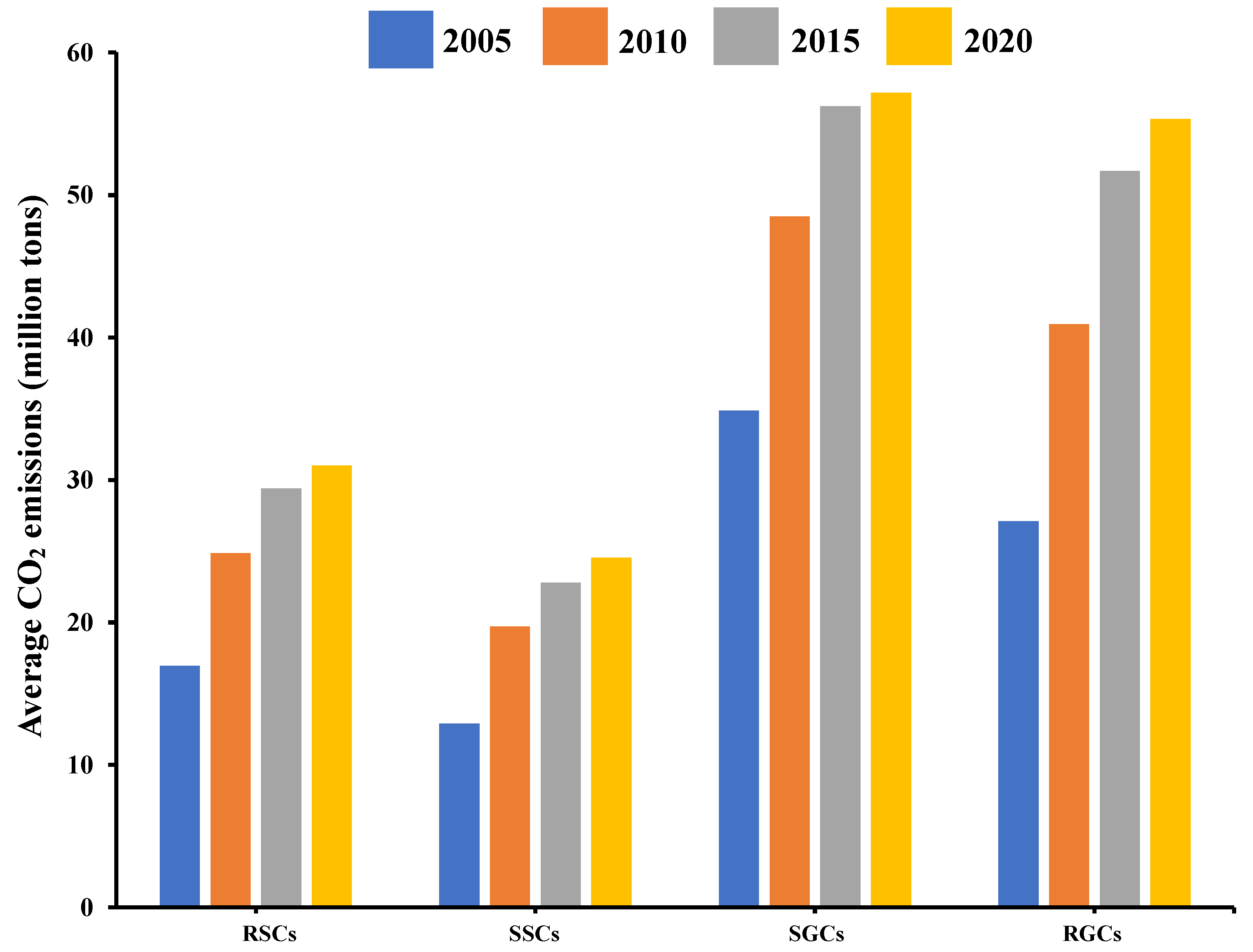
3.2. CO₂ Emission Patterns in Four Types of Cities

The spatiotemporal variations in city-level CO₂ emissions between 2005 and 2020 are provided in Figure 3. High-emission cities extended from the east to the middle and western regions and were mainly growing cities. In 2005, the number of growing cities with CO₂ emissions over 45 million tons was limited to four. In contrast, there were 65 such high-emission cities in 2020, including one shrinking city (Fuzhou). High-emission cities are mainly distributed in the northern, central, and eastern coastal areas, provincial capitals, and urban agglomerations in the west. With the highest CO₂ emissions, North and Central China are the main energy and industrial bases and major grain-producing areas. Moreover, the eastern coast is the most economically developed region in China, where human activities are intense, energy consumption is high, and manufacturing industries are densely distributed. In the west, high CO₂ emissions are concentrated near provincial capitals.

Considering each shrinking and growing city type as a statistical unit, the average CO₂ emissions of the four types of cities rose between 2005 and 2020 (Figure 4). Urban shrinkage does not necessarily indicate a reduction in CO₂ emissions. The average CO₂ emissions of shrinking cities increased nearly 2.5 times, while the average CO₂ emissions of growing cities increased nearly three times during 2005–2020. Moreover, the average CO₂ emissions growth rate showed a downward trend. The average annual growth rate of RSCs decreased from 7.97% between 2000 and 2010 to 1.47% between 2010 and 2015, and that of SSCs decreased from 7.97% to 1.47%. RGCs’ average annual growth rate decreased from 10.00% between 2000 and 2010 to 2.19% between 2010 and 2015; for SGCs, the average annual growth rate decreased from 10.18% to 1.64%.

3.3. Regression Results Using Panel Data Analysis

The panel regression model includes a number of measures, such as GDP, POP, PTI, PSI, NP, UA, COMP, and POLY, to investigate the patterns of CO₂ emissions in various types of growing and shrinking cities. The summary statistics for the major variables are displayed in

Table 3. Descriptive statistics of the variables.

City Type	STA	Variables
		CO2 (Million Tons)	POP (10 Thousand)	GDP (Billion RMB)	PTI	PSI	NP	UA (100 ha)	COMP	POLY
RSCs	Min	1.71	83.10	56.20	0.25	0.22	1.00	16.81	0.12	0.0001
	Max	16.59	586.20	1272.00	0.47	0.66	9.00	112.30	0.34	0.70
	Mean	25.56	197.50	362.70	0.35	0.42	4.56	46.88	0.20	0.41
	Std	20.49	143.90	309.30	0.05	0.12	2.50	25.65	0.05	0.24
SSCs	Min	1.70	44.52	34.55	0.09	0.02	1.00	4.79	0.10	0.00
	Max	77.46	913.50	4618.00	0.55	0.90	40.00	913.60	0.45	0.81
	Mean	20.34	309.90	671.00	0.36	0.45	5.62	113.90	0.24	0.41
	Std	14.73	155.60	736.10	0.08	0.12	5.68	160.70	0.06	0.28
SGCs	Min	1.64	5.50	35.07	0.07	0.15	1.00	1.90	0.04	0.00
	Max	334.87	3372.00	25,123.00	0.80	0.82	139.00	8458.00	0.45	0.93
	Mean	49.18	471.60	1320.00	0.36	0.47	10.46	221.90	0.26	0.44
	Std	45.92	371.20	2357.00	0.08	0.11	16.02	649.40	0.06	0.28
RGCs	Min	1.80	15.96	17.93	0.09	0.19	1.00	5.73	0.13	0.00
	Max	214.24	1466.00	18,100.00	0.76	0.80	49.00	8543.00	0.46	0.86
	Mean	44.36	490.80	1853.00	0.42	0.47	9.99	928.10	0.26	0.40
	Std	39.47	294.30	2679.00	0.11	0.11	10.03	2105.00	0.06	0.27

. The Levin, Lin, and Chu (LLC) test was then conducted to determine the stability of the panel data sequence (

Table 4. Results of the unit root test.

Variable	RSCs		SSCs		SGCs		RGCs
	Level	First Difference	Level	First Difference	Level	First Difference	Level	First Difference
CO2	−14.1259 ***	−6.3066 ***	−548.781 ***	−341.776 ***	−99.6230 ***	−65.3884 ***	−18.3833 ***	−12.2948 ***
POP	5.4545	2.3902 **	−54.0986 ***	−54.6276 ***	−689.514 ***	−708.287 ***	−60.7095 ***	−31.0693 ***
GDP	−3.0364 ***	−2.1956 ***	−8.4507 ***	−5.4990 ***	−20.8508 ***	−11.6829 ***	−1881.81 ***	−1046.42 ***
PTI	−0.5565	−4.9363 ***	−8.7341 ***	−9.4362 ***	−9.4974 ***	−13.2948 ***	−23.9084 ***	−27.7928 ***
PSI	−22.6488 ***	−32.7364 ***	−14.1487 ***	−17.1371 ***	−26.4779 ***	−21.7802 ***	−3665.26 ***	−5994.35 ***
NP	−17.4592 ***	−8.7742 ***	−19.8174 ***	−14.5465 ***	−53.5101 ***	−23.4148 ***	−37.0500 ***	−24.8638 ***
UA	−8.7721 ***	−6.2708 ***	−23.0802 ***	−15.6955 ***	−60.6931 ***	−40.8987 ***	−12.2519 ***	−9.2530 ***
COMP	−6.2836 ***	−5.5554 ***	−183.939 ***	−154.928 ***	−45.7696 ***	−46.1783 ***	−349.548 ***	−424.789 ***
POLY	−18.2298 ***	−10.4689 ***	−5.2708 ***	−7.7655 ***	−60.1365 ***	−39.8373 ***	−3.7859 ***	−8.0858 ***

Note: *** p < 0.01, ** p < 0.05.

); the rejection of the null hypothesis confirmed this. According to the LLC test, POP in RGCs was insignificant. Therefore, the non-stationary null hypothesis was accepted at that level; however, it was rejected at the first difference. At the least 10% significance level, the other variables were stationary.

Table 5. Results of the co-integration test.

City Type	Test Statistic	POP	GDP	PTI	PSI	NP	UA	COMP	POLY
RSCs	Panel v-Statistic	0.0233 **	1.1588	−0.1796 *	−0.3257	0.1409	0.8091	−0.0420	−0.3600 *
	Panel rho-Statistic	1.1940	−0.1067	1.2668	1.2346	0.5647	−0.0030	0.9625	1.1202
	Panel PP-Statistic	−0.4870 ***	−6.2019 ***	−0.1451 ***	−0.5165 *	−3.7068 ***	−3.7351 ***	−1.1019 ***	−1.6411 ***
	Panel ADF-Statistic	0.5263 ***	−4.1790 ***	0.8386 *	0.4470 ***	−2.1930 **	−2.1186 ***	−0.0604 **	−0.4227 **
	Group rho-Statistic	2.3502	1.3114	2.4982	2.2576	1.722	1.3447	1.8629	2.4004
	Group PP-Statistic	−0.5190 *	−9.4304 ***	0.2891 **	−10.1981 ***	−5.1926 ***	−4.8119 ***	−4.3731 ***	−1.4304 *
	Group ADF-Statistic	0.9773	−7.3724 ***	1.6253	−8.9027 ***	−4.1489 ***	−2.632 ***	−2.7326 ***	0.1852
SSCs	Panel v-Statistic	0.5183	3.6731 ***	0.2330	0.3807	−0.1447	1.847933 **	0.1005	0.8797
	Panel rho-Statistic	1.5005	0.6424	2.3077	2.3946	1.0868	0.7272	1.3449	0.6353
	Panel PP-Statistic	−6.5628 ***	−7.0976 ***	−3.0063 ***	−1.9615 ***	−1.1259 **	−4.4131 ***	−3.5623 ***	−1.7022 *
	Panel ADF-Statistic	−3.3356 ***	−3.5383 ***	−0.3000	0.5768	−0.0070 **	−4.3719 ***	−3.7483 ***	−0.4286 **
	Group rho-Statistic	4.1206	3.8750	4.9133	4.8789	2.3944	2.7657	3.2131	2.0398
	Group PP-Statistic	−16.4318 ***	−6.6553 ***	−11.1132 ***	−7.6012 ***	−0.3965 **	−4.2927 ***	−15.0044 ***	−4.9225 ***
	Group ADF-Statistic	−11.7374 ***	−2.3504 ***	−8.0367 ***	−3.5109 ***	0.8032 ***	−4.3719 ***	−16.6144 ***	−2.6010 ***
SGCs	Panel v-Statistic	0.3545 *	5.2307 ***	−1.0501	0.6953 **	−0.0096 ***	2.7254 ***	−0.6478	−0.2119 *
	Panel rho-Statistic	2.6512	2.7709	4.1462	4.1756	0.7091	0.4532	1.9871	1.1131
	Panel PP-Statistic	−14.3626 ***	−8.0537 ***	−7.4204 ***	−4.6069 ***	−1.9600 **	−5.6293 ***	−2.3451 ***	−0.3171 ***
	Panel ADF-Statistic	−8.0000 ***	−2.4717 ***	−2.3303 ***	0.1850 ***	−0.6346 ***	−2.7812 ***	−0.2455 *	0.7034 **
	Group rho-Statistic	7.4200	7.5964	9.5816	8.3656	1.8189	2.8536	3.6530	2.4189
	Group PP-Statistic	−25.1071 ***	−9.0558 ***	−13.6015 ***	−21.9617 ***	−1.8550 **	−5.3353 ***	−3.0976 ***	−0.2414 **
	Group ADF-Statistic	−17.1356 ***	−1.6227 *	−7.2152 ***	−14.2750 ***	−0.1329 **	−1.9289 **	−0.5820	1.1289
RGSs	Panel v-Statistic	0.8933	2.7484 ***	0.0388	−0.0760	−0.0184	2.5001 *	−0.0385	−0.4665 *
	Panel rho-Statistic	1.0837	1.5199	2.4011	2.6504	0.9108	0.7963	2.8926	1.1014
	Panel PP-Statistic	−6.8208 ***	−5.3587 ***	−3.5236 ***	−2.1224 ***	−1.2254 ***	−8.0178 ***	−1.1131 **	−1.2955 ***
	Panel ADF-Statistic	−3.3076 ***	−2.0595 ***	−0.5912 **	0.5777 *	−0.1858 **	−4.1134 ***	1.4930 *	−0.1453 **
	Group rho-Statistic	3.9707	4.2957	5.52591	5.2763	1.5765	3.8883	5.8570	2.4439
	Group PP-Statistic	−18.0738 ***	−5.6861 ***	−9.8851 ***	−12.7621 ***	−6.9114 ***	−10.0407 ***	−2.2354 **	−0.3732
	Group ADF-Statistic	−13.7984 ***	−1.4718 *	−6.0546 ***	−7.6607 ***	−5.2533 ***	−4.8353 ***	0.6664	0.8869 ***

Note: *** p < 0.01, ** p < 0.05, * p < 0.1.

shows the results of the co-integration test: the panel rho-statistics (within-dimension) and group rho-statistics (between-dimension) of all relevant variables of the four types of cities were not significant, and the null hypothesis without co-integration was accepted. Nevertheless, the other five statistics rejected that, at at least 10%, suggesting that CO₂ and the other independent variables co-integrated.

A panel regression model was developed based on the above tests in order to assess the influence of various urban forms and socioeconomic factors on CO₂ emissions. According to the F-test and Hausman test, the fixed-effects model was used for the estimation (

Table 6. Results of the F-test and Hausman test.

City Type	F-Test		Hausman Test
	F-Value	Prob	Chi-Sq. Statistic	Prob
RSCs	F = 14.5958	0.0000	27.1862	0.0000
SSCs	F = 137.5371	0.0000	10.9576	0.0224
SGCs	F = 22.6130	0.0000	44.2744	0.0000
RGCs	F = 15.0323	0.0000	70.6084	0.0000

). The model has achieved satisfactory regression results in RSCs, SSCs, SGCs, and RGCs with R-squared values greater than 0.9613 (

Table 7. Regression results.

Explanatory Variables	RSCs	SSCs	SGCs	RGCs
Ln(POP)	0.6660	0.4103 ***	0.4731 ***	0.6525 ***
Ln(GDP)	0.4526 ***	0.4811 ***	0.4952 ***	0.4483 ***
Ln(PTI)	−0.130	−0.2333	0.4902 ***	0.6956 ***
Ln(PSI)	0.3130	0.3678 ***	1.5973 ***	0.3546 *
Ln(NP)	0.3312 *	0.2922 ***	0.6650 ***	0.3700 ***
Ln(UA)	0.6290 ***	0.6736 ***	0.7273 ***	0.6608 ***
Ln(COMP)	−0.9142 **	−0.2998 *	−0.2723 *	0.4123 **
Ln(POLY)	−0.0062	−0.0040	−0.0084	0.0352 *
C	−6.7544	−0.5780 *	0.7102 ***	0.0167
R-squared	0.9842	0.9749	0.9694	0.9613
F	66.3428	94.3541	89.4942	62.3264
Number of obs	66	69	56	94

Note: *** p < 0.01, ** p < 0.05, * p < 0.1.

).

The regression results showed a significant positive correlation between the NP and CO₂ emissions, especially in SGCs. This indicates that cities with fragmented urban forms produce high CO₂ emissions; they enhance the dispersion of daily activities, resulting in increased urban production and living costs. Therefore, fragmented urban forms generate high CO₂ emissions, which is consistent with the findings of Ou et al. [52] and Yeh et al. [58].

In addition, as reported by Shi et al. [24] and Zheng et al. [59], UA promoted CO₂ emissions. UA was the main factor affecting CO₂ emissions in SSCs. The growth of urban areas implies that they are in the developmental stage of urban expansion, and the scientific management problems brought about by urban development planning cannot be solved on time within a certain period. The rapid development of urban industries has led to a substantial increase in urban CO₂ emissions.

In contrast, COMP inhibits CO₂ emissions in RSCs, SSCs, and SGCs but plays a promoting role in RGCs. COMP showed an evident effect on CO₂ emissions in RSCs; an increase of 1% in COMP decreased CO₂ emissions by 0.9142%. A high COMP indicates that the more regular the urban forms, the more conducive they are to reducing CO₂ emissions. Regular urban forms promote the development of public transportation and reduce the pressure on transportation and logistics transportation, thus showing a certain inhibitory effect on CO₂ emissions, which is consistent with the findings of Fang et al. [60], Wang et al. [23], and Liu et al. [61]. However, COMP was positively correlated with CO₂ emissions in RGCs; an increase in urban compactness aggravated CO₂ in RGCs. This may be because the more concentrated the inner city, the more energy consumption per capita will increase, leading to chaos in transportation network planning, traffic congestion, and other phenomena associated with the rapid development of cities. The energy consumed by residents in the commuting process due to urban traffic jams exceeds the energy saved by the reduction in travel distance caused by agglomeration.

In RSCs, SSCs, and SGCs, POLY inhibited CO₂ emissions while promoting CO₂ emissions in RGCs. POLY is significant only for gas-related energy consumption [28,61]. The development of polycentric spatial structures helps overcome the issues caused by the excessive agglomeration of single centers. In contrast, when a new center is developed, the “separation of occupation and residence” phenomenon is likely to increase urban commuting costs and promote CO₂ emissions. Our results show that higher polycentricity is usually associated with higher levels of CO₂ emissions in rapidly growing cities, which is consistent with the findings of Zhu et al. [62]. At the same time, in line with Sha, Chen [28] and Sun et al. [63], polycentric cities are often associated with low CO₂ emissions.

As reported by Shi et al. [22], Tong et al. [35], and Li et al. [64], POP, GDP, and PSI promoted CO₂ emissions. For SGCs, PSI had the most positive impact; every 1% increase in PSI increased CO₂ emissions by 1.5973%. The secondary industry is dominated by energy, iron and steel, construction, and other industries and consumes a large amount of energy and other resources in production and manufacturing processes. However, the evident positive effects on CO₂ emissions cannot be ignored.

Our results imply that the PTI inhibits CO₂ emissions in shrinking cities; however, it promotes CO₂ emissions in growing cities, which is consistent with the results of Tong et al. [35] and Wu et al. [65]. For shrinking cities, transforming urban industrial structures from industrial secondary industries to low-carbon and environmentally friendly tertiary industries can significantly reduce the intensity of CO₂ emissions. In contrast, for growing cities, the proportion of tertiary industries partially aggravates CO₂ emissions. Meanwhile, for RGCs; a 1% increase in PTI resulted in a 0.6956% increase in CO₂ emissions. A high PTI may be related to high urban consumption and services (e.g., shopping, tourism, commerce, and trade), resulting in an increase in CO₂ emissions.

We conducted the following tests to enhance the robustness of the results. First, the Chinese city-level CO₂ emissions data produced by Chen et al. [66] were calculated as the newly explained variable for the robustness analysis. County-level CO₂ emissions were estimated using nighttime light data. The data agreed with the CO₂ emissions based on the existing literature. They were therefore summed to obtain the city-level CO₂ emissions.

Table 8. Robustness test using an alternative for the explained variable.

Variables	RSCs	SSCs	SGCs	RGCs
Ln(POP)	4.0682	0.7845 *	0.3198 ***	0.6260 ***
Ln(GDP)	0.5205 ***	0.3045 ***	0.3576 ***	0.3864 ***
Ln(PTI)	−0.2869	−0.1373	0.3641 ***	0.5092 **
Ln(PSI)	0.0055	0.0109	0.7838 ***	0.4133 ***
Ln(NP)	0.3947	0.2558 *	0.4655 ***	0.1170
Ln(UA)	1.5783 ***	0.7603 ***	0.6399 ***	0.7002
Ln(COMP)	−0.7941	−0.1222	0.1243	0.3531
Ln(POLY)	−0.0406	−0.0550	−0.0049	0.0338
C	14.2849	−0.7452	6.6940 ***	7.2636 ***
R-squared	0.8746	0.9214	0.9344	0.9033
F-statistic	3.7191	18.3937	26.1489	15.1081
Number of obs	66	69	56	94

Note: *** p < 0.01, ** p < 0.05, * p < 0.1.

describes the regression results, similar to the original ones. Second, certain core cities have high preference status and financial capacity regarding economic vitality, policy priority, political orientation, etc. Therefore, the top three core cities (in economic development) of each type of city were eliminated to avoid interference from outliers. These cities were Suihua, Benxi, and Jixi in RSCs; Wenzhou, Daqing, and Anshan in SSCs; Shanghai, Beijing, and Tianjin in SGCs; and Guangzhou, Shenzhen, and Hangzhou in RGCs.

Table 9. Robustness test removing the top three core cities of each city group.

Variables	RSCs	SSCs	SGCs	RGCs
Ln(POP)	4.1779	0.3903 **	0.4656 ***	0.6334 ***
Ln(GDP)	0.4385 ***	0.4789 ***	0.4982 ***	0.4493 ***
Ln(PTI)	0.0366	−0.4271 **	0.4817 ***	0.6432 ***
Ln(PSI)	0.1542	0.3994 ***	1.6550 ***	0.5312 *
Ln(NP)	0.5828 **	0.3412 ***	0.6612 ***	0.3907 ***
Ln(UA)	1.2056 ***	0.6630 ***	0.7343 ***	0.6619 ***
Ln(COMP)	−0.7547	−0.3071	−0.2689 *	0.4007
Ln(POLY)	−0.0210	−0.0045	−0.0085	−0.0353
C	7.7363	0.1704	2.0692 ***	1.7183 ***
R-squared	0.9875	0.9738	0.9676	0.9615
F-statistic	45.9421	86.7761	83.0973	61.3479
Number of obs	63	66	53	91

Note: *** p < 0.01, ** p < 0.05, * p < 0.1.

shows the regression results after this removal, which remained highly robust, supporting their robustness.

3.4. Analysis of CO₂ Emissions in Shrinking Cities

The regression results in the RSCs and SSCs indicate that population, GDP, the proportion of secondary industry, and urban area have distinct promoting effects on CO₂ emissions. Population decline and economic recession are the main indicators of the shrinking of cities [67,68]. Considering that CO₂ emissions from shrinking cities continuously increased during the study period, it was inferred that the promotion effect of the development of secondary industry and urban areas on CO₂ emissions exceeded the mitigation effect of the decline of population and GDP on CO₂ emissions. The government has insisted on the importance of industrial upgrading in modernization by issuing policy documents to guide its path. However, the industrial transformation has not been successful in shrinking cities, with problems such as the low quality of the service industry and the incomplete transformation of the secondary industry. Yang et al. [69] indicated that the industrial production of shrinking cities is dominated by heavy industry. In contrast, the tertiary industry has a relatively low proportion and is mainly the transportation industry. Therefore, the economic development of shrinking cities requires an industrial structure dominated by secondary industry, which is closely dependent on fossil fuel consumption. Moreover, extensive industrialization constitutes the main driving force of CO₂ emissions in shrinking cities; to realize the coordinated development of their urban economy and ecology, it is necessary to actively change the industrial structure and develop high-technology industries with low energy consumption and pollution.

Meanwhile, the continuous expansion of built spaces during local population loss further aggravates urban CO₂ emissions. A reduction in urban population size can fundamentally reduce the demand for urban space, easing the pressure on energy consumption. However, in shrinking cities, local governments face high local financial pressures and often rely heavily on the land, thus boosting the spatial expansion of shrinking cities. The increase in built-up areas in shrinking cities has been the focus of several studies [70,71]. Wu et al. [72] revealed that urban expansion accompanied by low population density aggravates CO₂ emissions. The outmigration of the labor force leads to the continuous loss of the local population; the growth of construction land promotes the further expansion of built areas, resulting in the coexistence of population loss and urban expansion. The imbalance between population and urban land further worsens the profound problems of energy consumption, waste of land resources, and decay of the construction environment, aggravating the problem of CO₂ emissions. Therefore, attention should be paid to the unbalanced urbanization model of population and urban land to explore carbon reduction strategies that are suitable for the current situation of shrinking cities.

Based on the previous analysis, we provide the following suggestions for shrinking city policymakers: First, the proportion of tertiary industries should be increased while eliminating high-polluting industries as much as possible. Advanced technologies should be introduced, and the research and development of key technologies should be accelerated to improve carbon emission efficiency. Second, land resources should be used economically and intensively to avoid the disorderly expansion of urban land; achieving compact development should be prioritized. Moreover, the formulation and implementation of land use plans are advised to ensure the rational development of land, optimize land allocation, and increase green areas to achieve a low-carbon economy.

3.5. Analysis of CO₂ Emissions in Growing Cities

Rapid economic growth unavoidably leads to a rapid increase in urban CO₂ emissions for growing cities. In contrast to shrinking cities, the proportion of tertiary industries promotes the growth of CO₂ emissions, as indicated by the regression results. Secondary industries consume energy in production and manufacturing, and transferring the industrial structure to tertiary industries relieves the pressure on CO₂ emissions to a certain extent [73]. Along with the adjustment of the economic structure and the acceleration of industrial transformation, the position of the tertiary industry is becoming increasingly important, and its contribution rose steadily from 24.6% in 1978 to 54.5% in 2020. Although the tertiary industry is related to lower CO₂ emissions compared to the secondary industry, such emissions are increasing, and its influence is becoming increasingly evident in growing cities while its status is improving and its scope is expanding. Sun et al. [74] revealed that carbon emissions from tertiary industries increased from 382.54 million tons to 1406.46 million tons during 2003–2016, exceeding China’s average annual economic growth rate. The tertiary industry has become one of the core links and important carriers of energy consumption and CO₂ emissions in the development of the economy; however, blindly increasing the proportion of the tertiary industry cannot alleviate the pressure on CO₂ emissions. In the process of industrial transformation, the inhibitory effects of energy efficiency and industrial structure on CO₂ emissions cannot offset the growth of CO₂ emissions from tertiary industries; therefore, attention should be paid to the green and healthy development of tertiary industries.

In addition, the results show that urban areas play a significant role in promoting CO₂ emissions. With rapid urban expansion, urban green space has been largely invaded, reducing carbon sinks in growing cities. The increase in population, a key factor of scale expansion, is expected to accelerate energy consumption and increase CO₂ emissions through various intermediary mechanisms. Controlling urban land expansion should become the focus of future low-carbon cities. In addition, urban compactness and polycentricity accelerate CO₂ emissions in RGCs, which differ from other city groups. During rapid urbanization, uncoordinated spatial planning leads to excessive compactness and polycentricity. Zhang et al. [75] pointed out that compactness does not always reduce CO₂ emissions; excessive compactness exacerbates urban CO₂ emissions. Excessive compactness leads to the rapid transformation of other types of land use into construction land; that is, CO₂ source patches (e.g., energy consumption, industrial processes, and agricultural activities) are increasingly concentrated. In contrast, carbon sink patches (e.g., vegetation and water areas) are gradually more fragmented, thus increasing CO₂ emissions. Meanwhile, the housing area does not match the population size in the main city centers because of the population explosion. A significant number of inhabitants choose to live in sub-centers, thus forming new population centers and the need to commute long distances to work; this aggravates the imbalance between jobs and housing, extending the urban commuting distance, reducing its efficiency, and increasing CO₂ emissions. Jung et al. [76] reported that urban forms with high compositional polycentricity contribute to increased CO₂ emissions, which is consistent with the previous statement. Considering the negative effects of excessive agglomeration and polycentricity, adjusting and optimizing urban spatial structures has become a powerful path for rapidly growing cities.

Based on the previous analysis, we propose the following suggestions for the low-carbon development of growing cities. First, the government should promote the optimization and transformation of industrial structure, create a favorable environment for the rise of the tertiary industry, and vigorously develop modern service industries with low resource consumption and high added value, such as finance and information. Additionally, it is important to focus on making plans for upgrading the industrial structure while reducing resource consumption. Thereafter, relevant policies should be formulated to ensure rapid and healthy industry development and achieve a gradual reduction of CO₂ emissions. Second, urban compactness should be adjusted according to urban function and the stage of urban development. Geographical connectivity and functional cohesion among urban functional patches should be strengthened while optimizing urban compactness. Meanwhile, the right time to realize the transformation from single-center to multi-center development mode should be wisely selected to avoid weakening the agglomeration benefits of the single-center mode due to excessive multi-centers. While forming a multi-center development model suitable for the city’s overall layout, it is necessary to improve each center’s business environment and public service level, optimize the combination of functions within the city center, and ensure commuting efficiency between different urban centers.

4. Conclusions

In order to assist growing and shrinking cities in sustainable emission-reduction policies, this study explored how socioeconomic factors and urban forms interrelate to affect CO₂ emissions. For this purpose, 285 cities were divided into four categories based on a comprehensive index system: rapidly shrinking cities, slightly shrinking cities, slightly growing cities, and rapidly growing cities. In addition, Urban boundary data, Landscan datasets, and urban statistics were used to calculate the indicators representing socioeconomic factors and urban forms. Finally, a panel data regression model was constructed to explore the influence factors of CO₂ emissions in contexts of urban growth and shrinkage.

The parameter estimation from the selected panel data model showed that in terms of social economy, the proportion of secondary industry (PSI) had positive effects on CO₂ emissions, while the proportion of tertiary industry (PTI) had different effects on CO₂ emissions between growing and shrinking cities. PTI had negative effects on CO₂ emission in shrinking cities; however, it had a positive impact on growing cities. The results indicate that secondary industry remains the main driving force for economic development, which has significantly aggravated CO₂ emissions, while the rapid development of the tertiary industry has increasingly increased CO₂ emissions of growing cities. In terms of urban forms, urban size (UA) and fragmentation (NP) have positive effects on CO₂ emissions. Urban aggregation (COMP) and polycentricity (POLY) had negative effects on CO₂ emissions in shrinking and slightly growing cities; however, they had positive effects on CO₂ emissions in rapidly growing cities. The results show that the coexistence of population loss and space expansion is worthy of attention in shrinking cities. Meanwhile, despite urban agglomeration and urban polycentricity contributing to CO₂ emissions reduction, excessive agglomeration and polycentricity occur in rapidly growing cities, which significantly aggravates CO₂ emissions.

These findings suggest that policies to develop low-carbon cities in the future should take into account the different development patterns of urban growth and shrinkage and seize the opportunities of low-carbon transition. Shrinking cities should use land resources economically and intensively to avoid disorderly expansion of urban land and strive to achieve compact development. In addition, they should accelerate industrial transformation and eliminate high-polluting industries as much as possible. For growing cities, the government is advised to promote optimizing and transforming industrial structures and vigorously developing modern service industries with low resource consumption and high added value. Moreover, urban compactness and polycentricity should be adjusted according to urban functions and the stages of urban development. In addition, it is necessary to improve each center’s business environment and public service level and strengthen the geographical connectivity among urban functional patches.

Finally, the following issues should be addressed in future research. First, it is highly relevant to explore the influence of diverse industries, such as the secondary industries, traffic, and service industry, on CO₂ emissions to deepen energy conservation and emission reduction research. Second, urban spatial structure is a three-dimensional feature. Future studies may focus on the effects of horizontal and vertical spatial forms on CO₂ emissions. Third, it is essential to explore further the technologies employed in smart cities that aid in reducing CO₂ emissions in the case of growing and shrinking cities.

References

1. Laufkötter, C.; Zscheischler, J.; Frölicher, T.L. High-impact marine heatwaves attributable to human-induced global warming. Science 2020, 369, 1621–1625. [Google Scholar] [CrossRef] [PubMed]
2. Stephenson, D.B.; Diaz, H.; Murnane, R.J.C.E. Definition, diagnosis, and origin of extreme weather and climate events. In Climate Extremes and Society; Cambridge University Press (CUP): Cambridge, UK, 2009; Volume 340, pp. 11–23. [Google Scholar] [CrossRef]
3. Hay, J.; Mimura, N. The changing nature of extreme weather and climate events: Risks to sustainable development. Geomat. Nat. Hazards Risk 2010, 1, 3–18. [Google Scholar] [CrossRef]
4. Wu, W.; Ma, J.; Banzhaf, E.; Meadows, M.; Yu, Z.; Guo, F.; Sengupta, D.; Cai, X.; Zhao, B. Examining the relationship between urbanization and the eco-environment using a coupling analysis: Case study of Shanghai, China. Ecol. Indic. 2017, 77, 185–193. [Google Scholar] [CrossRef]
5. Ewing, R.; Bartholomew, K.; Winkelman, S.; Walters, J.; Anderson, G. Urban development and climate change. J. Urban. 2008, 1, 201–216. [Google Scholar] [CrossRef]
6. Wang, Z.; Yin, F.; Zhang, Y.; Zhang, X. An empirical research on the influencing factors of regional CO2 emissions: Evidence from Beijing city, China. Appl. Energy 2012, 100, 277–284. [Google Scholar] [CrossRef]
7. Shi, K.; Chen, Y.; Li, L.; Huang, C. Spatiotemporal variations of urban CO2 emissions in China: A multiscale perspective. Appl. Energy 2018, 211, 218–229. [Google Scholar] [CrossRef]
8. Begum, R.; Sohag, K.; Abdullah, S.; Jaafar, M. CO2 emissions, energy consumption, economic and population growth in Malaysia. Renew. Sustain. Energy Rev. 2015, 41, 594–601. [Google Scholar] [CrossRef]
9. Ozturk, I.; Acaravci, A. CO2 emissions, energy consumption and economic growth in Turkey. Renew. Sustain. Energy Rev. 2010, 14, 3220–3225. [Google Scholar] [CrossRef]
10. Shao, S.; Luan, R.; Yang, Z.; Li, C. Does directed technological change get greener: Empirical evidence from Shanghai’s industrial green development transformation. Ecol. Indic. 2016, 69, 758–770. [Google Scholar] [CrossRef]
11. Liu, Q.; Wu, S.; Lei, Y.; Li, S.; Li, L. Exploring spatial characteristics of city-level CO2 emissions in China and their influencing factors from global and local perspectives. Sci. Total Environ. 2021, 754, 142206. [Google Scholar] [CrossRef]
12. Liu, M.; Yang, X.; Wen, J.; Wang, H.; Feng, Y.; Lu, J.; Chen, H.; Wu, J.; Wang, J. Drivers of China’s carbon dioxide emissions: Based on the combination model of structural decomposition analysis and input-output subsystem method. Environ. Impact Assess. Rev. 2023, 100, 107043. [Google Scholar] [CrossRef]
13. Sheinbaum, C.; Ozawa, L.; Castillo, D. Using logarithmic mean Divisia index to analyze changes in energy use and carbon dioxide emissions in Mexico’s iron and steel industry. Energy Econ. 2010, 32, 1337–1344. [Google Scholar] [CrossRef]
14. Muñiz, I.; Rojas, C. Urban form and spatial structure as determinants of per capita greenhouse gas emissions considering possible endogeneity and compensation behaviors. Environ. Impact Assess. Rev. 2019, 76, 79–87. [Google Scholar] [CrossRef]
15. Apergis, N. Environmental Kuznets curves: New evidence on both panel and country-level CO2 emissions. Energy Econ. 2016, 54, 263–271. [Google Scholar] [CrossRef]
16. Tang, C.F.; Tan, B.W. The impact of energy consumption, income and foreign direct investment on carbon dioxide emissions in Vietnam. Energy 2015, 79, 447–454. [Google Scholar] [CrossRef]
17. Iwata, H.; Okada, K.; Samreth, S. Empirical study on the environmental Kuznets curve for CO2 in France: The role of nuclear energy. Energy Policy 2010, 38, 4057–4063. [Google Scholar] [CrossRef]
18. Allard, A.; Takman, J.; Uddin, G.S. The N-shaped environmental Kuznets curve: An empirical evaluation using a panel quantile regression approach. Environ. Sci. Pollut. Res. 2018, 25, 5848–5861. [Google Scholar] [CrossRef] [PubMed]
19. Awaworyi, C.; Inekwe, J.; Ivanovski, K.; Smyth, R. The Environmental Kuznets Curve in the OECD: 1870–2014. Energy Econ. 2018, 75, 389–399. [Google Scholar] [CrossRef]
20. Casey, G.; Galor, O. Population growth and carbon emissions. No. 22885. Natl. Bur. Econ. Res. 2016. Available online: http://www.nber.org/papers/w22885 (accessed on 1 October 2023).
21. Ou, J.; Liu, X.; Li, X.; Chen, Y. Quantifying the relationship between urban forms and carbon emissions using panel data analysis. Landsc. Ecol. 2013, 28, 1889–1907. [Google Scholar] [CrossRef]
22. Shi, K.; Xu, T.; Li, Y.; Chen, Z.; Gong, W.; Wu, J.; Yu, B. Effects of urban forms on CO2 emissions in China from a multi-perspective analysis. J. Environ. Manag. 2020, 262, 110300. [Google Scholar] [CrossRef]
23. Wang, M.; Madden, M.; Liu, X. Exploring the relationship between urban forms and CO2 emissions in 104 Chinese cities. J. Urban Plan. Dev. 2017, 143, 04017014. [Google Scholar] [CrossRef]
24. Shi, F.; Liao, X.; Shen, L.; Meng, C.; Lai, Y. Exploring the spatiotemporal impacts of urban form on CO2 emissions: Evidence and implications from 256 Chinese cities. Environ. Impact Assess. Rev. 2022, 96, 106850. [Google Scholar] [CrossRef]
25. Yi, Y.; Ma, S.; Guan, W.; Li, K. An empirical study on the relationship between urban spatial form and CO2 in Chinese cities. Sustainability 2017, 9, 672. [Google Scholar] [CrossRef]
26. Zuo, S.; Dai, S.; Ren, Y. More fragmentized urban form more CO2 emissions? A comprehensive relationship from the combination analysis across different scales. J. Clean. Prod. 2020, 244, 118659. [Google Scholar] [CrossRef]
27. Martinez-Fernandez, C.; Audirac, I.; Fol, S.; Cunningham-Sabot, E. Shrinking cities: Urban challenges of globalization. Int. J. Urban Reg. Res. 2012, 36, 213–225. [Google Scholar] [CrossRef] [PubMed]
28. Sha, W.; Chen, Y.; Wu, J.; Wang, Z. Will polycentric cities cause more CO2 emissions? A case study of 232 Chinese cities. J. Environ. Sci. 2020, 96, 33–43. [Google Scholar] [CrossRef] [PubMed]
29. Li, S.; Zhou, C.; Wang, S.; Hu, J. Dose urban landscape pattern affect CO2 emission efficiency? Empirical evidence from megacities in China. J. Clean. Prod. 2018, 203, 164–178. [Google Scholar] [CrossRef]
30. Döringer, S.; Uchiyama, Y.; Penker, M.; Kohsaka, R. A meta-analysis of shrinking cities in Europe and Japan. Towards an integrative research agenda. Eur. Plan. Stud. 2020, 28, 1693–1712. [Google Scholar] [CrossRef]
31. Schetke, S.; Haase, D. Multi-criteria assessment of socio-environmental aspects in shrinking cities. Experiences from eastern Germany. Environ. Impact Assess. Rev. 2008, 28, 483–503. [Google Scholar] [CrossRef]
32. Rieniets, T. Shrinking Cities: Causes and Effects of Urban Population Losses in the Twentieth Century. Nat. Cult. 2009, 4, 231–254. [Google Scholar] [CrossRef]
33. Sun, J.; Zhou, T. Urban shrinkage and eco-efficiency: The mediating effects of industry, innovation and land-use. Environ. Impact Assess. Rev. 2023, 98, 106921. [Google Scholar] [CrossRef]
34. Xiao, H.; Duan, Z.; Zhou, Y.; Zhang, N.; Shan, Y.; Lin, X.; Liu, G. CO2 emission patterns in shrinking and growing cities: A case study of Northeast China and the Yangtze River Delta. Appl. Energy 2019, 251, 113384. [Google Scholar] [CrossRef]
35. Tong, X.; Guo, S.; Duan, H.; Duan, Z.; Gao, C.; Chen, W. Carbon-Emission Characteristics and Influencing Factors in Growing and Shrinking Cities: Evidence from 280 Chinese Cities. Int. J. Environ. Res. Public Health 2022, 19, 2120. [Google Scholar] [CrossRef]
36. Wang, Y.; Guo, C.; Chen, X.; Jia, L.; Guo, X.; Chen, R.; Zhang, M.; Chen, Z.; Wang, H. Carbon peak and carbon neutrality in China: Goals, implementation path and prospects. China Geol. 2021, 4, 27. [Google Scholar] [CrossRef]
37. Wang, F.; Wu, M.; Zheng, W. What are the impacts of the carbon peaking and carbon neutrality target constraints on China’s economy? Environ. Impact Assess. Rev. 2023, 101, 107107. [Google Scholar] [CrossRef]
38. Deng, T.; Wang, D.; Yang, Y.; Yang, H. Shrinking cities in growing China: Did high speed rail further aggravate urban shrinkage? Cities 2019, 86, 210–219. [Google Scholar] [CrossRef]
39. Du, Z.; Li, X. Growth or shrinkage: New phenomena of regional development in the rapidly-urbanising Pearl River Delta. Acta Geoglogica Sin. 2017, 72, 1800–1811. [Google Scholar] [CrossRef]
40. Long, Y.; Wu, K. Shrinking cities in a rapidly urbanizing China. Environ. Plan. A Econ. Space 2016, 48, 220–222. [Google Scholar] [CrossRef]
41. Martinez-Fernandez, C.; Weyman, T.; Fol, S.; Audirac, I.; Cunningham-Sabot, E.; Wiechmann, T.; Yahagi, H. Shrinking cities in Australia, Japan, Europe and the USA: From a global process to local policy responses. Prog. Plan. 2016, 105, 1–48. [Google Scholar] [CrossRef]
42. Wiechmann, T.; Pallagst, K. Urban shrinkage in Germany and the USA: A comparison of transformation patterns and local strategies. Int. J. Urban Reg. Res. 2012, 36, 261–280. [Google Scholar] [CrossRef]
43. Elzen, M.; Fekete, H.; Höhne, N.; Admiraal, A.; Forsell, N.; Hof, A.; Olivier, J.; Roelfsema, M.; van Soest, H. Greenhouse gas emissions from current and enhanced policies of China until 2030: Can emissions peak before 2030? Energy Policy 2016, 89, 224–236. [Google Scholar] [CrossRef]
44. Long, Y.; Song, Y.; Chen, L. Identifying subcenters with a nonparametric method and ubiquitous point-of-interest data: A case study of 284 Chinese cities. Environ. Plan. B Urban Anal. City Sci. 2022, 49, 58–75. [Google Scholar] [CrossRef]
45. Cai, B.; Cui, C.; Zhang, D.; Cao, L.; Wu, P.; Pang, L.; Zhang, J.; Dai, C. China city-level greenhouse gas emissions inventory in 2015 and uncertainty analysis. Appl. Energy 2019, 253, 113579. [Google Scholar] [CrossRef]
46. Jiang, H.; Sun, Z.; Guo, H.; Xing, Q.; Du, W.; Cai, G. A standardized dataset of built-up areas of China’s cities with populations over 300,000 for the period 1990–2015. Big Earth Data 2022, 6, 103–126. [Google Scholar] [CrossRef]
47. Sun, Z.; Du, W.; Jiang, H.; Weng, Q.; Guo, H.; Han, Y.; Xing, Q.; Ma, Y. Global 10-m impervious surface area mapping: A big earth data based extraction and updating approach. Int. J. Appl. Earth Obs. Geoinf. 2022, 109, 102800. [Google Scholar] [CrossRef]
48. Wang, X.; Li, Z.; Feng, Z. Classification of Shrinking Cities in China Based on Self-Organizing Feature Map. Land 2022, 11, 1525. [Google Scholar] [CrossRef]
49. Zhang, X.; Zhang, Q.; Zhang, X.; Gu, R. Spatial-temporal evolution pattern of multidimensional urban shrinkage in China and its impact on urban form. Appl. Geogr. 2023, 159, 103062. [Google Scholar] [CrossRef]
50. Buhnik, S. From Shrinking Cities to Toshi no Shukushō: Identifying Patterns of Urban Shrinkage in the Osaka Metropolitan Area. Berkeley Plan. J. 2012, 23, 132–155. [Google Scholar] [CrossRef]
51. Oswalt, P.; Rieniets, T. Atlas of Shrinking Cities; Jones: Berlin, Germany, 2006; pp. 22–25. [Google Scholar]
52. Ou, J.; Liu, X.; Wang, S.; Xie, R.; Li, X. Investigating the differentiated impacts of socioeconomic factors and urban forms on CO2 emissions: Empirical evidence from Chinese cities of different developmental levels. J. Clean. Prod. 2019, 226, 601–614. [Google Scholar] [CrossRef]
53. Liu, Y.; Song, Y.; Song, X. An empirical study on the relationship between urban compactness and CO2 efficiency in China. Habitat Int. 2014, 41, 92–98. [Google Scholar] [CrossRef]
54. Liu, X.; Wang, M. How polycentric is urban China and why? A case study of 318 cities. Landsc. Urban Plan. 2016, 151, 10–20. [Google Scholar] [CrossRef]
55. Xiao, Y.; Huang, H.; Qian, X.; Zhang, L.; An, B. Can new-type urbanization reduce urban building carbon emissions? New evidence from China. Sustain. Cities Soc. 2023, 90, 104410. [Google Scholar] [CrossRef]
56. Asici, A.A. Economic growth and its impact on environment: A panel data analysis. Mpra Paper 2013, 24, 324–333. [Google Scholar] [CrossRef]
57. Xie, Q.; Wu, H. How does trade development affect environmental performance? New assessment from partially linear additive panel analysis. Environ. Impact Assess. Rev. 2021, 89, 106584. [Google Scholar] [CrossRef]
58. Yeh, A.G.-O.; Li, X. A constrained CA model for the simulation and planning of sustainable urban forms by using GIS. Environ. Plan. B Plan. Des. 2001, 28, 733–753. [Google Scholar] [CrossRef]
59. Zheng, S.; Huang, Y.; Sun, Y. Effects of urban form on carbon emissions in china: Implications for low-carbon urban planning. Land 2022, 11, 1343. [Google Scholar] [CrossRef]
60. Fang, C.; Wang, S.; Li, G. Changing urban forms and carbon dioxide emissions in China: A case study of 30 provincial capital cities. Appl. Energy 2015, 158, 519–531. [Google Scholar] [CrossRef]
61. Liu, X.; Wang, M.; Wei, Q.; Wu, K.; Wang, X. Urban form, shrinking cities, and residential carbon emissions: Evidence from Chinese city-regions. Appl. Energy 2020, 261, 114409. [Google Scholar] [CrossRef]
62. Zhu, K.; Tu, M.; Li, Y. Did polycentric and compact structure reduce carbon emissions? A spatial panel data analysis of 286 Chinese cities from 2002 to 2019. Land 2022, 11, 185. [Google Scholar] [CrossRef]
63. Sun, B.; Han, S.; Li, W. Effects of the polycentric spatial structures of Chinese city regions on CO2 concentrations. Transp. Res. Part D Transp. Environ. 2020, 82, 102333. [Google Scholar] [CrossRef]
64. Li, Z.; Wang, F.; Kang, T.; Wang, C.; Chen, X.; Miao, Z.; Zhang, L.; Ye, Y.; Zhang, H. Exploring differentiated impacts of socioeconomic factors and urban forms on city-level CO2 emissions in China: Spatial heterogeneity and varying importance levels. Sustain. Cities Soc. 2022, 84, 104028. [Google Scholar] [CrossRef]
65. Wu, D.; Zhou, D.; Zhu, Q.; Wu, L. Industrial structure optimization under the rigid constraint of carbon peak in 2030: A perspective from industrial sectors. Environ. Impact Assess. Rev. 2023, 101, 107140. [Google Scholar] [CrossRef]
66. Chen, J.; Gao, M.; Cheng, S.; Hou, W.; Song, M.; Liu, X.; Liu, Y.; Shan, Y. County-level CO2 emissions and sequestration in China during 1997–2017. Sci. Data 2020, 7, 391. [Google Scholar] [CrossRef] [PubMed]
67. Rhodes, J.; Russo, J. Shrinking ‘smart’?: Urban redevelopment and shrinkage in Youngstown, Ohio. Urban Geogr. 2013, 34, 305–326. [Google Scholar] [CrossRef]
68. Yang, Z. Sustainability of urban development with population decline in different policy scenarios: A case study of Northeast China. Sustainability 2019, 11, 6442. [Google Scholar] [CrossRef]
69. Yang, S.; Yang, X.; Gao, X.; Zhang, J. Spatial and temporal distribution characteristics of carbon emissions and their drivers in shrinking cities in China: Empirical evidence based on the NPP/VIIRS nighttime lighting index. J. Environ. Manag. 2022, 322, 116082. [Google Scholar] [CrossRef]
70. Hu, Y.; Wang, Z.; Deng, T. Expansion in the shrinking cities: Does place-based policy help to curb urban shrinkage in China? Cities 2021, 113, 103188. [Google Scholar] [CrossRef]
71. Qiang, W.; Lin, Z.; Zhu, P.; Wu, K.; Lee, H.F. Shrinking cities, urban expansion, and air pollution in China: A spatial econometric analysis. J. Clean. Prod. 2021, 324, 129308. [Google Scholar] [CrossRef]
72. Wu, Y.; Li, C.; Shi, K.; Liu, S.; Chang, Z. Exploring the effect of urban sprawl on carbon dioxide emissions: An urban sprawl model analysis from remotely sensed nighttime light data. Environ. Impact Assess. Rev. 2022, 93, 106731. [Google Scholar] [CrossRef]
73. Zhou, X.; Zhang, J.; Li, L. Industrial structural transformation and carbon dioxide emissions in China. Energy Policy 2013, 57, 43–51. [Google Scholar] [CrossRef]
74. Sun, Y.; Qian, L.; Liu, Z.; Yu, D. The carbon emissions level of China’s service industry: An analysis of characteristics and influencing factors. Environ. Dev. Sustain. 2021, 24, 13557–13582. [Google Scholar] [CrossRef]
75. Zhang, H.; Peng, J.; Wang, R.; Zhang, J. Spatial planning factors that influence CO2 emissions: A systematic literature review. Urban Clim. 2021, 36, 100809. [Google Scholar] [CrossRef]
76. Jung, M.; Kang, M.; Kim, S. Does polycentric development produce less transportation carbon emissions? Evidence from urban form identified by night-time lights across US metropolitan areas. Urban Clim. 2022, 44, 101223. [Google Scholar] [CrossRef]
Figure 1. The spatial distribution of the study areas.
Sustainability 16 00085 g001
Figure 2. Geographical distribution of the four types of cities.
Sustainability 16 00085 g002
Figure 3. The spatiotemporal variations in city-level CO2 emissions between 2005 and 2020.
Sustainability 16 00085 g003
Figure 4. Average CO2 emissions between the four city groups from 2005 to 2020.
Sustainability 16 00085 g004