Abstract
Economic dispatch, emission dispatch, or their combination (EcD, EmD, EED) are essential issues in power systems optimization that focus on optimizing the efficient and sustainable use of energy resources to meet power demand. A new algorithm is proposed in this article to solve the dispatch problems with/without considering wind units. It is based on the Social Group Optimization (SGO) algorithm, but some features related to the selection and update of heuristics used to generate new solutions are changed. By applying the highly disruptive polynomial operator (HDP) and by generating sequences of random and chaotic numbers, the perturbation of the vectors composing the heuristics is achieved in our Modified Social Group Optimization (MSGO). Its effectiveness was investigated in 10-unit and 40-unit power systems, considering valve-point effects, transmission line losses, and inclusion of wind-based sources, implemented in four case studies. The results obtained for the 10-unit system indicate a very good MSGO performance, in terms of cost and emissions. The average cost reduction of MSGO compared to SGO is 368.1 $/h, 416.7 $/h, and 525.0 $/h for the 40-unit systems. The inclusion of wind units leads to 10% reduction in cost and 45% in emissions. Our modifications to MSGO lead to better convergence and higher-quality solutions than SGO or other competing algorithms.
1. Introduction
The power generation sector has been undergoing continuous development in recent years, with a focus on diversification of energy sources and production technologies, but also on efficiency and constant innovation. Decision makers aim through regulations and policies to create a competitive and attractive framework for investors while ensuring the sustainable development of the energy system [1]. In order for electricity producers and companies to remain in a competitive market, it is necessary for them to operate with the lowest possible costs and to use sources/technologies with the lowest possible environmental impact. One way to optimize operating costs while taking emissions into account is to solve the economic emission dispatch (EED) problem [2]. The goal of the EED problem is to determine the optimal operating mode of energy sources to minimize the two objectives—cost and emissions—considering a given power demand, as well as the operating limits of the generating units [3]. If the EED problem aims only at cost optimization (without considering emissions), then this is called the economic dispatch problem (EcD) [4]. If EED only aims to optimize emissions (without considering costs), then it is called the emission dispatch (EmD) problem [5]. For a more complete approach, both the economic aspects and the level of emissions released into the atmosphere must be taken into account, which implies solving the EED problem.
Initially, the solution to EcD, EmD, and EED problems focused mainly on conventional unit power plants (firing coal, gas, etc.), as they had a very large share of the power system structure. However, last year’s warnings about the environmental impact of these types of power plants led to an increased use of both high-efficiency co-generation units (CU) (that simultaneously produce both electricity and heat), and renewable energy power generation systems (RESPSs) to steer the electricity generation sector towards sustainable development [6,7]. The EED problem that includes CU aims at the optimal scheduling (in terms of cost and emissions) of power-only units, heat-only units, and their combination: co-generation units [8]. It is a similar situation for EcD [9] or EmD [8] problems, with both aiming to manage all categories of units operating in the power system: power-only, heat-only, and CU units. For systems that include CU units, in addition to costs and constraints specific to power-only units, the EED optimization model must also consider the fuel costs related to heat-only and CU units, power-heat dependencies, and the produced-demand heat balance [10]. In the case of including RESPSs in the power system, an important option is the use of wind energy, which can be converted into electricity without producing greenhouse gases. Wind energy is considered a renewable and clean energy source, having only a low secondary impact on the environment due to the manufacturing process of the equipment and its transport. Increasing the share of wind energy in the energy mix has a positive impact on the quality of the environment and reduces dependence on conventional sources. Since wind is an uncontrollable and variable source of energy, the energy production from wind units is influenced by weather conditions and wind speed. Thus, the operation of power systems that include wind units must also take into account the unpredictable variations in the power of these units [4].
The integration of wind units into EcD, EmD, or EED problems brings challenges related to wind speed distribution, mathematical optimization models, and solution algorithms. One of the most common parametric distributions used in wind speed modeling is the Weibull distribution [11,12,13], but other distributions can be considered, such as [14] Gamma, inverse Gamma, Gaussian, Burr, Halphen, etc.
In the following, some articles are presented which propose mathematical models and solution algorithms for solving EcD, EmD, or EED problems considering the uncertainties caused by unpredictable wind speed fluctuations. Thus, in [4], an optimization model is presented that includes the costs related to the overestimation and underestimation of the wind power. The case study considers a Weibull distribution of the wind speed, and it shows that the optimal solutions to the EcD problem can be influenced by factors associated with the overestimation and underestimation of wind power. Based on a linear relationship between wind speed and wind power, and considering a Weibull distribution for wind speed, in [11], an optimization model is developed for the minimization of emissions, in which the uncertainty of the wind power is included in the constraints of the model. In [12], both the cost of emissions and the cost of overestimation and underestimation of wind power are included in the bi-objective EED problem. Starting from the classical formulation of EcD and EmD problems, in [2], the objective functions related to costs and emissions are extended with terms that include the uncertainty of the wind power. The resulting models are tested on a system consisting of two conventional units and two wind units, considering a mixed Gamma-Weibull distribution for the wind speed. To solve the EED problem with the inclusion of wind power, in [15], the Honey Bee Mating Optimizer (HBMO) is applied, where a so-called 2m-point model is used to estimate the uncertainty of the wind power. In [16], a new evolutionary technique called Lightning Flash Algorithm (LFA) is proposed to solve the bi-objective EED problem by considering different levels of wind power penetration and multiple fuel sources. The LFA technique is efficient for the EED problem, having a good convergence and achieving lower costs and emissions than other algorithms. A robust and efficient optimization model for dispatching wind-thermal power under uncertainties is developed in [1], taking into account robustness, economics, and environmental aspects. In [17], another robust model for the optimization of the EcD problem is presented. It is based on the identification of a set of discrete bad scenarios, where the objective function aims at minimizing all the penalties associated with the bad scenarios.
The EcD, EmD, or EED problems that include or do not include wind power uncertainty are non-convex with multiple local optima and nonlinear constraints [12,15,16] requiring advanced solution algorithms.
For the study of both systems (the ones comprising conventional-only units and the ones comprising thermal-wind units), several algorithms are presented in the following lines. Considering the first category of systems, in [18], an Improved Class Topper Optimization (ICTO) has been developed by including in the classical CTO three new concepts: adaptive improvement factor, adaptive acceleration coefficient, and chaos local search, which help to enhance the exploration and exploitation capability of the ICTO. The ICTO is tested on five systems with conventional units, and it performs better, in terms of cost and emissions, than the original CTO and several other competing algorithms. A quasi-oppositional-based political optimizer is used, in [19], to solve the bi-objective EED problem considering valve-point loading effect, transmission line losses, and other constraints related to conventional units. Recently, two new population-based algorithms (Criminal Search Optimization Algorithm (CSOA) [20] and Kho-Kho optimization algorithm (KKO) [21]) have been developed and applied to solve the EED problem. Both algorithms (CSOA and KKO) show good exploitation and exploration capabilities, and they can be used to solve complex problems in various domains. Another option for solving the EED problem is presented in [22], where two metaheuristic algorithms, Exchange Market Algorithm (EMA) and Adaptive Inertia Weight Particle Swarm Optimization (AIWPSO), are combined to obtain a new algorithm with improved global and local search abilities. The constraints of the EED problem are maintained using the multiple constraints ranking technique. The best compromise solution (BCS) obtained using EMA-AIWPSO dominates the BCSs obtained using other algorithms (such as KKO, ISA, or GSA). Also, several multi-objective algorithms have been proposed for solving the EED problem, such as multi-objective SSA [23], multi-objective cultural algorithm [24], NSGA-III algorithm [25], or multi-objective quasi-oppositional TLBO [26], each of which uses a basic metaheuristic algorithm (SSA, CA, GA, or TLBO) that is endowed with the Pareto-dominance principle to generate successive Pareto fronts. The multi-objective algorithms mentioned [23,24,25,26] have been tested on various power systems with conventional units, their performance being superior to other recognized multi-objective techniques (MODE, NSGA II, or SPEA-2).
Over the time, when trying to solve the EED problem, various techniques have been used to optimally program the units of the thermal-wind systems. Thus, in [6], the techniques of weighted goal programming and the progressive bounded constraint method are combined to generate a set of Pareto solutions that are efficient in the cost–emission space, and then extract the best compromise solution. For instance, four cases are analyzed to quantify and demonstrate the benefits of including wind units in the structure of a power system comprising only thermal units. In [12], the Artificial Bee Colony (ABC) algorithm is strengthened by including the best solution in the update equations, and in [27], chaos is inserted into the sine–cosine algorithm to obtain better-quality solutions to the EED problem. Additionally, in [13]—where wind units are considered—a number of eight metaheuristic algorithms (Flower Pollination Algorithm (FPA), Mine Blast Algorithm (MBA), Backtracking Search Algorithm (BSA), Symbiotic Organisms Search (SOS), Ant Lion Optimizer (ALO), Moth-Flame Optimization (MFO), Stochastic Fractal Search (SFS), and Lightning Search Algorithm (LSA)) are applied to identify the best solutions to the EcD, EmD, or EED problem. The FPA and BSA algorithms provide the best scheduling of thermal/wind units for cost and/or emission minimization. To study the behavior of systems in which thermal, wind, and solar units operate, in [28], the Dragonfly Algorithm (DA) is proposed for the EcD problem. Uncertainties related to the power generated by using wind and solar energy are modeled using the 2-m point estimation technique. The DA algorithm outperforms other algorithms, such as Crow Search Algorithm (CSA), Ant Lion Optimizer (ALO), oppositional RCCRO, Biogeography-Based Optimization (BBO), PSO, and GA, in terms of cost and execution time.
SGO is a metaheuristic algorithm proposed relatively recently by Satapathy SC (2016) [29], which is based on the fact that a social group of individuals has a greater ability to solve a real-life problem than a single individual. For some mathematical functions, SGO is more efficient than other well-known metaheuristic algorithms (such as [29]: DE, PSO, ABC, GA, TLBO, etc.), being an easy-to-implement algorithm, having two main phases (improving phase and acquiring phase) and a single specific parameter. However, for some mathematical functions or applications, it can provide a low performance due to an imbalance between exploration and exploitation, which ultimately leads to getting stuck in a local optimum [30]. Also, SGO may suffer due to the reduced diversity of the population [31]. To overcome the mentioned shortcomings and to obtain better quality solutions, there have been attempts to improve the performance of SGO by different strategies, such as modifying the relations for updating the solutions [30], inertia weight strategies [32], and hybridizations with other algorithms [31].
In this paper, some changes have been made to the original SGO algorithm, aiming to increase efficiency, resulting in the MSGO algorithm. In order to improve the exploration–exploitation balance, the commutation condition between the equations for updating the solutions in the acquiring phase was changed. Also, to increase the diversity of the population, a logistic map and a highly disruptive polynomial operator were inserted.
The main contributions of this paper are:
- We propose a modified version of SGO (called MSGO) in which the way of updating and adapting the individuals in the social group is changed by inserting chaos and an HDP operator (in the original SGO only uniformly randomly generated number sequences are used). The operators associated with chaos and HDP aim at increasing the efficiency of the MSGO algorithm by reducing the number of close solutions and overcoming some drawbacks related to slow convergence. To the best of the authors’ knowledge the HDP operator has never been used to improve the performance of the SGO algorithm.
- Implementation of MSGO to solve EcD, EmD, and EED problems with or without consideration of wind units.
- Conducting experiments to evaluate and statistically compare the effectiveness of MSGO with SGO and other well-known algorithms (or their varieties) for thermal or wind-thermal power systems of different sizes and characteristics.
2. Statement of the EcD, EmD, and EED Problems
2.1. Statement of the EcD Problem
The EcD problem for a power system that includes thermal and wind units aims to determine the power outputs of these generating units so that the operating cost of the entire system is minimized, and a number of technical constraints are met. For the formulation of the mathematical optimization model, we consider a power system comprising Nt thermal units and Nw wind units, and the total power demand (PD) of the consumers in the system is considered known and constant for the period of analysis. The variables to be optimized are continuos, being represented by the output power vectors of the thermal units PT = [PT1, PT2,…, PTi,…, PTNt] and of wind units PW = [PW1, PW2,…, PWj,…, PWNw].
The objective function C(PT, PW) is represented by two components; one related to the fuel cost of the thermal units, CT(PT), and the other related to the operating cost of the wind units, CW(PW) [4]:
where, CTi(PTi) is the fuel cost corresponding to thermal unit i, and CWj(PWj) is the operating cost corresponding to the wind unit j.
In this paper, the relationship between the fuel cost CTi(PTi) and output power PTi of a thermal unit i is modeled via a non-convex function consisting of a quadratic and a sinusoidal term [33]:
The operating cost of wind unit j, CWj(PWj), consists of three terms [4]: the direct operating cost of unit j (), the cost corresponding to the overestimation of the wind power (), and the cost corresponding the underestimation the wind power ().
The wind power overestimation for unit j occurs if the estimated wind power for this unit PWj is higher than the available power represented by a random variable Wj. In this situation, the difference between the two powers is covered by a reserve source and implies the reserve cost . In the opposite situation of the underestimation (if PWj is less than Wj), a part of the available power of unit j remains unused, which implies a penalty cost . Since Wj is a random variable, the powers and will include the uncertainty of the wind power, and their calculation method is presented below.
For the calculation of the average powers and , it is considered that the wind speed is modeled by a Weibull distribution whose probability density function (pdf) is given by relation (5) [11]:
where, V is the random variable wind speed, v denotes the wind speed (a value of V), and fV(v) is the pdf of the variable V, k is the shape parameter, and c is the scale parameter.
Also, between the random variable wind power (W) and the random variable wind speed (V), we consider a linear relationship expressed as follows [11]:
The use of the linear model (6) requires knowledge of three limit speeds: cut-in wind speed (vin), rated wind speed (vr), and cut-out wind speed (vout). PWr is the rated output power of the wind unit, which corresponds to the speed vr.
The pdf for wind power (W) over the continuous interval (0, PWr) has the expression:
where R = (vr − vin)/vin. Given relation (6) and the Weibull distribution of the wind speed, the event probabilities W = 0 and W = PWr are calculated using relations [4]:
Prob(W = 0) = Prob(V < vin) + Prob(V > vout) = 1 − exp[−(vin/c)k] + exp[−(vout/c)k]
Prob(W = PWr) = Prob(vr < V < vout) = exp[−(vr/c)k] − exp[−(vout/c)k]
We must say that, in general, the distributions of the variables V and W, as well as the pdfs derived from them, differ depending on the location of the wind turbine units. Thus, for wind unit j, the average powers associated with the overestimation and the underestimation of the wind power are mathematically expressed as follows [4]:
where is probability density function for the random variable having the form given by relation (7), while w are the values of the continuous random variable . The discrete probabilities and Prob(), for unit j, are calculated using relations (8) and (9), where represents rated wind power for unit j.
In Table A1 are presented the steps to evaluate the cost related to wind power, as well as a calculation example for a wind unit.
The feasible space of EcD problem solutions is limited by the following constraints [4,12]:
- The thermal units i must be operated between the minimum capacity (PTmin,i) and the maximum capacity (PTmax,i):
PTmin,i ≤ PTi ≤ PTmax,i, i = 1, 2,…, Nt
If the power of the thermal unit i in the previous hour is known or specified (), then the operating limits are given by the constraint:
where DRi and URi are the down-ramp and up-ramp limits of the unit i.
- 2.
- The wind units j must be operated between the minimum (PWmin,j) and maximum (PWmax,j) capacity:
PWmin,j ≤ PWj ≤ PWmax,j, j = 1, 2,…, Nw
- 3.
- The actual powers generated by the thermal and wind units must cover the power consumed in the system:
2.2. Statement of the EmD Problem
The EmD problem has a high level of similarity with the EcD problem, aiming to determine the PT and PW vectors, so that the emissions released into the atmosphere is minimal while maintaining some technical constrains at the units and system level. Thus, in the EmD problem, the variables to be optimized (PT and PW vectors), as well as the constraint relations (12)–(15), are identical to those in the EcD problem. The objective function is represented by the total amount of emissions released into the atmosphere, mathematically defined by the following relation [2]:
where (PTi) and ET(PT) represent the pollutant emissions released into the atmosphere due to the operation of thermal unit i, respective of all thermal units in the analyzed power system. (PWj) and EW(PW) are the pollutant emissions produced due to the need to use other thermal units to cover the uncertainty of the availability of wind unit j, respective of all wind units considered. Average powers, and , are calculated with relations (10) and (11), which include the uncertainty of wind power in the estimation of pollutant emissions.
The term represents the emissions released into the environment due to the need to use some thermal units in the system to cover the difference between the scheduled power of the wind unit PWj (power that cannot be realized due to the unavailability of the wind resource) and its available power (the case of overestimation of wind power). The term represents the emissions released into the environment by other thermal units due to the non-use of the full available power of wind unit j (the case of underestimation of wind power). The quantity of emissions released into the atmosphere by a thermal unit i can be defined by relation [2]:
2.3. Statement of the EED Problem
The EED problem is similar to the EcD and EmD problems, in that the variables to be optimized and the constraints of the problem are the same, but the objective function is different. In the EED problem, the objective function Φ(PT, PW) can be formed by the weighted and normalized summation of the cost C(PT, PW) and emissions E(PT, PW) objectives [34]:
where Cmin, Cmax are the minimum and maximum costs corresponding to the function C(PT, PW); Emin, Emax are the minimum and maximum emissions corresponding to the function E(PT, PW); ω and (1 − ω) are weighting factors associated with the normalized cost and emissions objectives, 0 ≤ ω ≤ 1.
To use relation (20) it is necessary to calculate the minimum (Cmin and Emin) and maximum (Cmax and Emax) values for the two objectives. The determination of the minimum values (Cmin, Emin) is done by first solving the EcD and EmD problems formulated in Section 2.1 and Section 2.2. The maximum values (Cmax, Emax) are determined while considering that the EcD and EmD problems have opposite tendencies [35]. Thus, the solution for which a minimum cost is obtained in the EcD problem will be considered to result in maximum emissions, and vice versa.
In current practice, system operators or decision makers look for a single solution that takes into account both objectives, which is generally the best compromise solution. By solving the EED problem for different values of the ω factor, one can estimate the set of non-dominant solutions that form the discrete Pareto front [5] (from which the BCS between the two objectives is extracted). To extract the BCS from the set of solutions belonging to the Pareto front, a fuzzy approach is used [5]. Thus, the solutions in the Pareto front are ordered according to one of the objectives, then for each objective i and non-dominant solution s, a fuzzy membership function μi,s is assigned. This is defined by relation [5]: μi,s = (fi,max − fi,s)/(fi,max − fi,min), i = {1, 2} and s = {1, 2,…, P}, where fi,min and fi,max are the minimum and maximum value of the ith objective function; fi,s is the value of the objective function corresponding to solution s and objective i; P is the number of non-dominated solutions from the Pareto front. In order to demonstrate the merit of all the objectives corresponding to solution s, the normalized membership function is calculated [5]:
The BCS corresponds to the maximum value of the index : μmax = Max(, s = 1, 2,…, P).
3. The Modified SGO Algorithm
3.1. Classic SGO
The SGO is a metaheuristic, population-based algorithm that is inspired by human social group behavior and is used for solving complex problems [29]. In the SGO, the population consists of a social group of N individuals Xi = [x1,i, x2,i,…, xj,i,…, xn,i]|i = 1, 2,…, N interacting and exchanging knowledge with each other, each individual representing a solution Xi to the problem. The characteristics of the individuals represent the components xj,i, j = 1, 2,…, n (n is the number of characteristics of an individual, which equals the size of the problem to be solved) of the solutions Xi, and the ability of an individual to find a solution to the problem is measured by the fitness function fi = f(Xi). The SGO algorithm has three phases: initialization phase, improving phase, and acquiring phase. In the initialization phase, each component xj,i, j = 1, 2,…, n of the solution Xi, is randomly generated between the minimum (xmin,j) and maximum (xmax,j) limits:
where r1 is a random number uniformly distributed in the range (0, 1).
xj,i = xmin,j + r1(xmax,j − xmin,j)
In the improving phase, each individual Xi, i = 1, 2,…, N of the group seeks to improve their traits xj,I by interacting with the best individual of the group at that moment, Xbest = [x1best, x2best,…, xjbest,… xnbest]. Thus, the new traits (xj,inew) of the individual Xinew are determined with relation [29]:
where c is the self-introspection parameter with values between 0 and 1, and r2 is a uniformly generated random number in the range (0, 1). If the new vector Xinew is better, then it is retained; otherwise, the old solution is kept.
xnewj,i = c xj,i + r2 (xjbest − xj,i)
In the acquiring phase, each individual Xi aims to improve its traits (level of knowledge) through mutual, cumulative interactions with both the best individual Xbest and an individual randomly r (r ≠ i) chosen from the population, Xr = [x1,r, x2,r,…, xj,r,…, xn,r]. Depending on the quality of the individuals Xi and Xr, the new traits (xj,inew) of the individual Xinew are determined as follows [29]:
If f(Xi) < f(Xr) Then
xj,inew = xj,i + r3 (xj,i − xj,r) + r4 (xjbest − xj,i)
Else
where, r3 and r4 denote independent arbitrary value in the (0, 1).
xj,inew = xj,i + r3 (xj,r − xj,i) + r4 (xjbest − xj,i)
The solutions obtained using the SGO algorithm are iteratively improved using the updating relations from the improving and acquiring phases, until the maximum number of iterations tmax is reached. A pseudo-code of the SGO algorithm is presented in detail in [29].
3.2. Modified SGO (MSGO)
The proposed MSGO algorithm includes the same phases as the original SGO algorithm, but some features of SGO have been modified to increase the efficiency of the MSGO algorithm. Two of these changes, presented below, aim at inserting two operators (one chaotic type and the other being highly disruptive polynomial (HDP)) in the structure of the solutions update relations to improve MSGO’s ability to escape from local minima and obtain better quality solutions.
Chaotic operator: Chaos, due to its properties (unpredictability, non-periodic, ergodicity, non-converging, pseudo-randomness etc. [18]), has been successfully incorporated into the structure of various optimization algorithms (such as adaptive sparrow search algorithm [36] and moth–flame optimizer [37]) to cover a number of shortcomings related to low population diversity, slow convergence of the optimization process, stagnation in a local area etc. In this paper, chaos is included in the MSGO algorithm using a chaotic sequence (cxp) generated by Logistic map [37] which can be effective in solving some EcD problems [18]. The Logistic map is defined by relation [18]:
where {cxp}p = 1…∞ represents the chaotic sequence generated by the Logistic map, at the pth iteration. The initial conditions are cx0 ∈ (0, 1) and cx0 ≠ {0.0, 0.25, 0.5, 0.75, 1}.
cxp+1 = 4 cxp (1 − cxp), cxp ∈ (0, 1)
HDP operator: In case of more complex mathematical functions, SGO cannot provide an efficient search in the whole solutions space by relying only on randomly generated sequences through numbers (r1–r4) or on randomly extracting a solution from the population (Xr). As a result, in order to increase the exploration and exploitation capacity of the MSGO algorithm, as well as the chances of exceeding local minima, a perturbation based on the HDP operator [38] is introduced into MSGO. Mathematically, the HDP operator is defined by relation [38]:
where, ru is a random number uniformly generated in the range [0, 1]; LBi and UBi indicate the lower and upper boundary of the variables xj,i; η is the index for the polynomial operator; α is a control parameter that is considered to have a value of 0.5 [39] (in this paper, the values of the parameter α are determined by experimental trials in the range (0, 1)); δH is the equation that alternates moderate values with high values for δ, while δL is the equation that generates low values for δ; δ1 and δ2 are calculated, based on the LBi and UBi imposed boundaries for the variable xj,i, with the relations δ1 = (xj,i − LBi)/(UBi − LBi) and δ2 = (UBi − xj,i)/(UBi − LBi).
In general, the HDP operator is used as a mutation operator that intervenes in altering some xj,i values of a Xi solution with a certain predetermined probability. In MSGO, the HDP operator is not used as a mutation operator, but as an operator applied to modify each variable xj,i of a solution Xi (practically, the mutation probability is considered equal to 1). Thus, depending on the HDP parameters (η, ru, δ1, α), the δ values generated by (26) may be high, which could cause some of the xj,i components of some Xi solutions to reach the limits of the search space relatively quickly (the δ values could generate excessively large search steps). To avoid this problem, the δ values generated by (26) will be attenuated/smoothed according to the current iteration t, if δ exceeds a certain limit value (δmax):
Figure 1 shows the first 10,000 values of δ generated by relation (26), considering the following settings for the HDP operator parameters: δ1 = rnd(1), δ2 = 1 − δ1; η = 4, α = 0.5, δmax = 1.5. The δH values generated by (26) under the condition ru ≤ α = 0.5 are marked in blue, and the δL values in red. Since the δH values are much higher than δL, in order to have a clearer picture, the δL values have been detailed in a separate graph on the interval (1, 10,000). It is seen that the δH equation alternates moderate values and high ones, while the δL equation generates only low values. Figure 2 shows the attenuated δa values obtained using (27). Initially, the δa values are higher (being able to ensure an efficient search in the whole solutions space), then with the increase in the number of simulations they attenuate, the search step is reduced, making the transition from exploration to exploitation, and at the end of the process the values are equal to or lower than the δmax limit (which facilitates the exploitation phase).
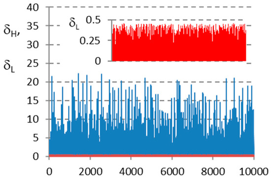
Figure 1.
HDP values generated for δH and δL.
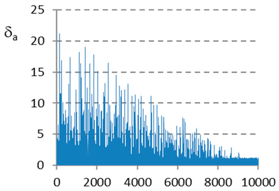
Figure 2.
The attenuated values obtained for δa.
The changes implemented in MSGO compared to SGO are presented below:
- The improving phase of MSGO is similar to that of SGO but the sequences of numbers r2 randomly generated in SGO by (23) are replaced by sequences of numbers generated by the attenuated DHP operator δa by relation (27) in the form:
- b.
- The acquiring phase of MSGO is similar to that of SGO, except for the following three modifications:
- b1.
- The sequences of numbers r3 randomly generated in SGO by (24a) are replaced by sequences of numbers generated by the attenuated DHP operator δa by relation (27).
- b2.
- The sequences of numbers r3 randomly generated in SGO by (24b) are replaced by chaotic sequences (cx) generated by the Logistic map with relation (25).
- b3.
- In SGO, switching between relations (24a) and (24b) is performed by considering the fitness of the competitive solutions Xi and Xr, based on the condition f(Xi) < f(Xr). In MSGO, this condition is replaced by a random one, having the form rnd(1) < β, where rnd(1) is a uniformly generated random number in the range (0, 1); β is a value determined by experimental trials.
The three changes (b1)–(b3) made in MSGO are embodied in relations (29a) and (29b):
If rnd(1) < β Then
xj,inew = xj,i + δa (xj,i − xj,r) + r4 (xjbest − xj,i)
Else
xj,inew = xj,i + cx (xj,r − xj,i) + r4 (xjbest − xj,i)
In Algorithm 1, the calculation steps for applying the MSGO algorithm are presented in detail, with the modifications (b1)–(b3) mentioned above.
| Algorithm 1: MSGO algorithm |
|
{Initialization phase} Initialize the iterations (t = 0), t is counter of iterations; Initialize the solutions Xi, i = 1, 2,…, N using relation (22); Evaluate the initial solutions and identify the best Xbest solution; repeat t = t + 1 For i = 1 To N Do {improving phase} For j = 1 To n Do Generate a value δ of the HDP operator using (26); Determine δa using relation (27); Update the components xj,i using relation (28), obtaining the new solution Xinew; End For j If the new solution Xinew is better, then it is retained; otherwise, the old solution is maintained; Find the best Xbest solution from the population; End For i For i = 1 To N Do {acquiring phase} Randomly select a solution Xr, rϵ{1, 2,…, N}, r ≠ i; If rnd(1) < β Then For j = 1 To n Do Generate a value δ of the HDP operator using (26); Determine δa using relation (27); Update xj,i using (29a), obtaining Xinew; End For j; End If Else For j = 1 To n Do Generate a chaotic value cx using (25); Update xj,i using (29b), obtaining Xinew; End For j; End Else If the new solution Xinew is better, then it is retained; otherwise, the old solution is maintained; Find the best Xbest solution from the population; End For i Until t ≥ tmax {stopping criterion} The best solution Xbest and the fitness f(Xbest) are retained. |
The main steps of the MSGO algorithm are summarized in a flowchart shown in Figure 3.
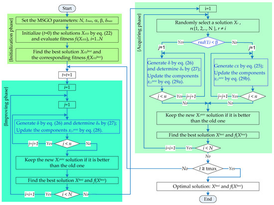
Figure 3.
Flowchart of the MSGO algorithm.
4. Implementing the MSGO for the EcD, EmD, or EED Problems
This section shows how to implement the MSGO algorithm for solving EcD, EmD, or EED problems. The application of MSGO for solving EcD, EmD, or EED problems is similar, the difference being given by the type of objective function to be minimized: cost C(PT, PW) defined by (1) for EcD problems, emission E(PT, PW) defined by (16) for EmD problems or Ф(PT, PW) defined by (20) for EED problems. For the implementation of the MSGO algorithm, a solution i is considered to be represented by the vector PTWi = [PTW1,i, PTW2,i,…, PTWj,i,…, PTWNt+Nw,i]|i = 1, 2,… N which includes the powers of thermal units (PTWj,i|j = 1,2,… Nt) and wind units (PTWj,i|j = Nt+1, Nt+2,…, Nt+Nw). If the system contains only thermal units, then the vector PTWi consists only of the powers generated by these units. We also denote PTWbest(t) as the best solution obtained using MSGO up to iteration t.
4.1. Stages of MSGO Implementation for the EcD, EmD, or EED Problem
The MSGO algorithm applied to solve the EcD, Em, or EED problems formulated in Section 2 includes the following steps:
- Step 1: Specify test system input data for the EcD, EmD, or EED problem: the number of thermal (Nt) and wind (Nw) units; cost coefficients for the thermal units (a, b, c, e, f); parameters (c, k) to the Weibull distribution; the characteristic values of the wind speed (vin, vr, vout); the rated output power of the wind units (PWr); active power limits for thermal and wind units (PTmin, PTmax; PWmin, PWmax); the cost coefficients (cd, co, cu) and emissions coefficients (eo, eu) to the wind units; the B-loss coefficients (Bij, B0i, B00); load demand (PD) and accuracy ε.
- Step 2: Set the parameters of the MSGO algorithm: N and tmax;
- Step 3: Random initialization of a population of N solutions, represented by the vectors PTWi|i = 1, 2,… N
- 3.1: t = 0;
- 3.2: Chaotic sequence cx are initialized using the logistic map;
- 3.3: Randomly generate an initial population with N solutions (PTWi(0)|i = 1,2,…, N) using relation (22). Each solution respects the constraints defined by relations (12)–(14); The constraint (14) is handled by a heuristic procedure CHM presented in Section 4.2;
- 3.4: Evaluate the initial solutions PTWi(0)|i = 1,2,…, N using relation (1), (16) or (20) associated with the EcD, EmD, or EED problems;
- 3.5: Find the best initial solution PTWbest(0) and the objective function associated with the addressed problem (EcD, EmD, or EED).
For t = 1 Do tmax
- Step 4: Update solutions PTWi(t)|i = 1,2,…, N in the improving phase.
- 4.1: For i = 1 To N Do
- 4.2: For j = 1 to n Do
- 4.3: Generate a value δ of the HDP operator using (26);
- 4.4: Determine δa using relation (27);
- 4.5: Updating the components PTWj,i(t) using relation (28), obtaining the new components PTWj,inew(t), at iteration t;
- 4.6: Checking the inequality constraints (12) and (13): if the PTWj,inew(t) power is outside the limits, then CHM from Section 4.2 is applied; End For j;
- 4.7: Checking the equality constraint (14): the new solution PTWinew(t) is adjusted using the equality constraint handling mechanism from Section 4.2;
- 4.8: Evaluate the new solution PTWinew(t) using relation (1), (16) or (20) depending on the addressed problem (EcD, EmD or EED): If the new solution PTWinew(t) is better, then it is retained; otherwise, the old solution is maintained;
- 4.9: Update the best solution PTWbest(t); End For i;
- Step 5: Update solutions PTWi(t)|i = 1,2,…, N in the acquiring phase.
- 5.1: For i = 1 To N Do
- 5.2: Randomly select a solution PTWr(t), rϵ{1, 2,…, N }, r ≠ i;
- 5.3: If rnd(1) < β Then
- 5.4: For j = 1 to n Do
- 5.5: Generate a δ value of the HDP operator using (26);
- 5.6: Determine δa using relation (27);
- 5.7: Updating PTWj,i(t) using (29a), getting the new components PTWj,inew(t) of the new solutions PTWinew(t);
- 5.8: Apply the procedure for handling inequality constraints (12) and (13) from Section 4.2; End For j; End If
- 5.9: Else
- 5.10: For j = 1 to n Do
- 5.11: Generate a chaotic value cx by (25);
- 5.12: Updating PTWj,i(t) by (29b), obtaining PTWj,inew(t);
- 5.13: Apply CHM from Section 4.2 for constraints (12) and (13); End For j; End Else
- 5.14: Checking the equality constraint (14): the new solution PTWinew(t) is adjusted using the equality constraint handling mechanism from Section 4.2;
- 5.15: Evaluate the new solution PTWinew(t) using relation (1), (16) or (20) depending on the addressed problem (EcD, EmD, or EED): if the new solution PTWinew(t) is better, then it is retained; otherwise the old solution is maintained;
- 5.16: Update the best solution PTWnew(t); End For i;
- Step 6: Stop the process: the calculation process is stopped when the maximum number of iterations (tmax) is reached. {End For t}
- Step 7: Memorize the best solution: The best solution PTWbest and the objective function associated with the problem addressed (EcD, EmD, or EED).
4.2. Constraints Handling Mechanism (CHM)
The CHM refers to the adjusting method of the solutions that do not satisfy the inequality and equality constraints of the EcD, EmD, or EED problems defined by relations (12)–(14). In the case of inequality constraints, defined by relations (12) and (13), if the power of a thermal or wind unit is outside the imposed operating limits (PTmin or PTmax, and PWmin or PWmax, respectively), then the power of this unit is set with the exceeded limit [40]. To handle the equality constraint, defined by (14), we apply a CHM procedure presented in [41]. The CHM(PTW) procedure has a single parameter, represented by the power vector PTW, and finally it returns a feasible solution that respects relation (14) with the imposed error ε. The CHM(PTW) is called whenever a PTW vector is updated in the initializing, the improving, or the acquiring phases of the MSGO or SGO algorithms.
5. Case Studies
The efficiency of the MSGO algorithm was tested on medium-sized (10-unit) and large (40-unit) systems, having different characteristics, such as operating limits of the units, transmission line losses, valve-point effect, wind power. According to the characteristics of the systems, four cases were studied, described below.
- Case 1 (C1): This case analyses a 10-unit system taking into account the transmission line losses. The power demand is 2000 MW. The cost coefficients (ai, bi, ci, ei, fi, i = 1, 2,…, 10), B-loss coefficients (Bij), and emission coefficients (αi, βi, γi, ηi, δi) are taken from [42].
- Case 2 (C2): The second case is a system having 40 units that considers the valve-point effects. The system is analyzed without considering transmission line losses. The power demand is 10,500 MW. The cost coefficients are considered from [33] and emission coefficients are provided by [43].
- Case 3 (C3): The case C3 is a system with 40 units similar to case C2 (the cost and emission coefficients are identical to those in case C2 [33,43]), but transmission losses are considered, as well. The power demand is 10,500 MW. The B-loss coefficients are taken from [44].
- Case 4 (C4): A 40-unit system derived from case C3 by replacing the first two thermal units (PT1 and PT2) with the two wind units (PW1 and PW2). Each wind unit has a nominal power of 550 MW, and the minimum and maximum capacities are PWmin,1 = PWmin,2 = 0, PWmax,1 = PWmax,2 = 550 MW. The power demand is PD = 10,500 MW. We consider that the wind speed has a Weibull distribution. The shape and scale parameters (k, c) corresponding to the sites of the two wind units have the values [13]: k1 = 1.5; c1 = 15; k2 = 1.5; c2 = 15. Other wind-related characteristics have the following values [13]: cut-in wind speed (vin = 5 m/s), rated wind speed (vr = 15 m/s), cut-out wind speed (vout = 45 m/s), the cost coefficients associated with underestimation () and overestimation (). The cost and emission coefficients for the thermal units (P3–P40) and the B-loss coefficients are identical to those mentioned in C3 case, being taken from [44]. The characteristics of the thermal units and the B-loss coefficients for the 10-unit and 40-unit systems are presented in Appendix A, Table A2, Table A3, Table A4 and Table A5.
Each of the cases mentioned in Table 1 (C1–C4) were studied based on the mathematical optimization models (presented in Section 2) of the problems EcD (cases C1a–C4a), EmD (cases C1b–C4b), and EED (cases C1c–C4c). The SGO and MSGO algorithms perform 50 independent runs for each case study, retaining four statistical indicators: Best cost/emission (B), Average cost/emission (A), Worst cost/emission (W), and the standard deviation (SD). Algorithms SGO and MSGO have been implemented in MathCAD and run on a PC with an Intel i5 processor, 2.2 GHz CPU and 4 GB of RAM.
5.1. Setting the Parameters
Adjusting the parameters of metaheuristic algorithms is an essential task with multiple positive effects, such as improved performance, adaptation of the algorithms to a specific problem, better execution times, and stability, etc. The proposed MSGO algorithm has three specific parameters (α, β, and δmax). A procedure based on the design of an experimental plan is used to set the specific parameters. They are successively set (for example, in the following order α, β, and δmax), starting from a set of initial values [45]. Thus, one parameter is varied, and the others are fixed either with the initial values or with the already set values. This procedure allows the evaluation of the MSGO algorithm performance through testing different combinations of the interest parameter values, followed by the selection of the best combination based on a predetermined criterion. The test values considered for setting the specific parameters are α = {0, 0.25, 0.5, 0.75, 1}, β = {0, 0.25, 0.5, 0.75, 1}, and δmax = {1.2, 1.5, 2}. The initial values are α = 0, β = 0, and δmax = 1.2. The parameter selection criterion is based on Average cost/emission obtained from 25 runs for each case study. Note that the experimental analysis does not guarantee the best values for the parameters of MSGO algorithm. However, the results obtained using MSGO following this selection process show that the algorithm parameters were reasonably set Table 1 shows the parameters of the MSGO algorithm (N, tmax, α, β, δmax) for all the analyzed cases.

Table 1.
Characteristics of the analyzed systems and values set for the SGO and MSGO parameters.
Table 1.
Characteristics of the analyzed systems and values set for the SGO and MSGO parameters.
| Cases | Type of Problem | SGO and MSGO | MSGO Parameters | PL | VPE | Wind | |||||
|---|---|---|---|---|---|---|---|---|---|---|---|
| n | N | tmax | NE | α | β | δmax | |||||
| C1a | EcD | 10 | 15 | 30 | 900 | 0.75 | 0.25 | 1.2 | √ | √ | - |
| C1b | EmD | 10 | 15 | 30 | 900 | 0.75 | 0.25 | 1.2 | √ | √ | - |
| C1c | EED | 10 | 15 | 30 | 900 | 0.75 | 0.25 | 1.2 | - | √ | - |
| C2a | EcD | 40 | 50 | 350 | 35,000 | 0.05 | 0.5 | 1.2 | - | √ | - |
| C2b | EmD | 40 | 50 | 350 | 35,000 | 0.05 | 0.5 | 1.2 | - | √ | - |
| C2c | EED | 40 | 50 | 350 | 35,000 | 0.05 | 0.5 | 1.2 | √ | √ | - |
| C3a | EcD | 40 | 50 | 350 | 35,000 | 0.05 | 0.5 | 1.5 | √ | √ | - |
| C3b | EmD | 40 | 50 | 200 | 20,000 | 0.05 | 0.5 | 1.5 | √ | √ | - |
| C3c | EED | 40 | 50 | 350 | 35,000 | 0.05 | 0.5 | 1.5 | √ | √ | - |
| C4a | EcD-Wind | 40 | 50 | 350 | 35,000 | 0.05 | 0.5 | 1.5 | √ | √ | √ |
| C4b | EmD-Wind | 40 | 50 | 200 | 20,000 | 0.05 | 0.25 | 1.5 | √ | √ | √ |
| C4c | EED-Wind | 40 | 50 | 350 | 35,000 | 0.05 | 0.5 | 1.5 | √ | √ | √ |
In the case of the SGO algorithm, the values of the common parameters (N and tmax) are the same as the values set for the MSGO algorithm in each case analyzed (these are shown in Table 1). The SGO algorithm has only one specific parameter c, the value of which being set to the one recommended in [29] (c = 0.2). For the fair comparison of the SGO and MSGO algorithms, the number of evaluations of the objective functions (NE) is considered equal in all analyzed cases (C1–C4), which is mentioned in Table 1.
5.2. Results for EcD (Cases C1a–C4a) and EmD (Cases C1b–C4b) Problems
The best solutions obtained using SGO and MSGO: The optimal scheduling of the thermal units for the cases C1a, C1b (10 units), and C2a, C2b (40 units) obtained using the MSGO and SGO algorithms are presented in Table 2 and Table 3, respectively.
Table 2.
Generation schedule obtained using SGO and MSGO for cases C1a, C1b, and C1c (PD = 2000 MW).
Table 3.
Generation schedule obtained using SGO and MSGO for cases C2a, C2b, and C2c (PD = 10,500 MW).
In the cases C1a and C1b, the system being of relatively small sizes, the MSGO and SGO algorithms find approximately the same optimal operating solution, and as a result, the derived quantities (Cost, Emission, PL) will be approximately the same. However, mathematically, MSGO performs slightly better than SGO. Thus, in the case of C1a the best costs obtained using MSGO and SGO are CostC1a(MSGO) = 111,497.6301 $/h and CostC1a(SGO) = 111,497.6302 $/h, respectively. For the C1b case, the best emissions found by MSGO and SGO are EmissionC1b(MSGO) = 3932.2432 lb/h and EmissionC1b(SGO) = 3932.2433 lb/h, respectively. Also, in the case of C2b (Table 3), the best solutions (P1–P40, Cost, Emission) found by MSGO and SGO are very close (both algorithms have the ability to identify quality solutions): EmissionC2b(MSGO) = 176,682.26363 t/h and EmissionC2b(SGO) = 176,682.26364 t/h, respectively.
On the contrary, in the case of C2a (where the functions that model the cost have a higher complexity and determine a larger number of local minima), the MSGO algorithm can identify a much better solution than SGO (CostC2a(MSGO) = 121,426.7039 $/h < CostC2a(SGO) = 121,509.8209 $/h).
Table 4 shows the best solutions in terms of cost and emissions obtained using the MSGO algorithm for the cases C3a, C3b (without wind), C4a, and C4b (with wind).
Table 4.
Generation schedule obtained using MSGO for cases C3a, C3b, and C3c (with loss of power and without wind) and C4a, C4b, C4c (with loss of power and wind).
The solutions for C4a and C4b cases indicate that the two wind units (PW1, PW2) are scheduled to operate at full capacity (550 MW) in both the EcD and EmD problems. Thus, according to the statement in case C4, the wind units will replace two thermal units PT1, PT2 (that operate at maximum capacity PT1 ≈ PT2 ≈ 114 MW in C3a and C3b cases), and will also reduce the operating power level of other thermal units (PT3–PT40). Based on the EcD and EmD models, it can be seen that if the wind units operate at full capacity it results in an power very close to zero (), so their corresponding costs and emissions will be close to zero. In contrast, the average powers associated with overestimation will tend towards maximum values , while their corresponding costs and emissions are 2 × 1153.817 $/h, and 2 × 1153.817 t/h. The risks taken by the system operator when planning the wind units to operate at values close to the maximum capacity are covered by the reduction of costs and emissions from the thermal units (due to the reduction of the PT3–PT40 powers in C4a(C4b) cases compared to C3a(C3b)).
Comparing the solutions for the cases with wind and those without wind, it can be seen that the inclusion of the wind units (PW1 and PW2) results in a substantial reduction in cost (from CostC3a(MSGO) = 136,454.33693 $/h to CostC4a(MSGO) = 123,161.88666 $/h, representing 9.74%), and emissions (from EmissionC3b(MSGO) = 347,578.49052 t/h to EmissionC4b(MSGO) = 193,311.54070 t/h representing 44.38%). Also, power losses are reduced from 958.62 MW in the case of C3a to 936.70 MW in the case of C4a (2.28%) and from 1040.54 MW in the case of C3b to 1009.74 MW in the case of C4b (2.96%), respectively.
Comparison of MSGO algorithm with other algorithms: In Table 5, Table 6, Table 7, Table 8, Table 9, Table 10, Table 11 and Table 12 the values of the statistical items (B, A, W, and SD) are presented. They are obtained using different algorithms for EcD problem (cases C1a–C4a) and EmD problem (C1b–C4b), respectively.
Analyzing the values from the mentioned tables, it can be seen that in all studied cases the MSGO algorithm obtains statistical indicators as good or better than the competing algorithms mentioned in these tables. The exception is the Worst cost item for the algorithms Jaya-SML [46] (case C2a—Table 6), ORCCRO [47] (case C3a—Table 7), DE (case C4a—Table 8), and the SD item for the algorithms CSS [48] (cases C3a—Table 7), DE, and SCA (cases C4a—Table 8).
The MSGO algorithm shows a better performance than well-known algorithms, such as DE [49], RCCRO [35] (in cases C1a—Table 5 and C1b—Table 9), GA [50], DE [42], ABC [51], PSO [52], TLBO [53], SCA [54], CSO [55] (cases C2a—Table 6), DE [26], TLBO [26], BSA [56] (cases C2b—Table 10), ACS [57], BBO [47], ORCCRO [47], CSS [48], IMO [58] (cases C3a—Table 7), PSO, DE, SCA (cases C3b—Table 11, C4a—Table 8, C4b—Table 12). Also, the performance of MSGO is superior to other metaheuristic algorithms obtained using various procedures (such as modification of solution update relations, inclusion of chaos and/or opposite solutions, hybridizations, etc.): GQPSO [59], CSCA [27], QOPO [19] (in cases C1a—Table 5), MIMO [58], HSCA [60], CTLBO [53], TLABC [61] (cases C2a—Table 6), GAAPI [44], SDE [62], HPSO-DE [63], MIMO [58] (cases C3a—Table 7).
Table 5.
Values for the statistical items obtained using different algorithms for the cases C1a—Best Cost (10 units with losses, 2000 MW).
Table 5.
Values for the statistical items obtained using different algorithms for the cases C1a—Best Cost (10 units with losses, 2000 MW).
| Algorithm | Best Cost ($/h) | Average Cost ($/h) | Worst Cost ($/h) | SD ($/h) | Cost Saving * ($/h) |
|---|---|---|---|---|---|
| DE [49] | 111,500 | - | - | - | - |
| TLBO [26] | 111,500 | - | - | - | - |
| QOTLBO [26] | 111,498 | - | - | - | - |
| QPSO [59] | 119,005.3030 | 121,621.7556 | 122,144.8454 | 372 | 10,124.12 |
| GQPSO [59] | 112,429.7444 | 113,102.4627 | 113,327.0680 | 256 | 1604.83 |
| RCCRO [35] | 111,497.6319 | - | - | - | - |
| BSA [56] | 111,497.6308 | - | - | - | - |
| CSCA [27] | 111,497.6307 | - | - | - | - |
| QOPO [19] | 111,892.4096 | - | - | - | - |
| SGO | 111,497.6302 | 111,497.7362 | 111,502.7703 | 7.27 × 10⁻¹ | 0.10 |
| MSGO | 111,497.6301 | 111,497.6302 | 111,497.6304 | 6.25 × 10⁻⁵ | 0 |
* Indicates the cost saving through MSGO compared to other algorithms using the Average Cost item.
Table 6.
Values of the statistical items obtained using different algorithms for the cases C2a—Best Cost (40 units without losses, 10,500 MW).
Table 6.
Values of the statistical items obtained using different algorithms for the cases C2a—Best Cost (40 units without losses, 10,500 MW).
| Algorithm | Best Cost ($/h) | Average Cost ($/h) | Worst Cost ($/h) | SD ($/h) | Cost Saving ($/h) |
|---|---|---|---|---|---|
| MIMO [58] | 122,758.7 | 124,621.8 | 126,059.2 | 866.20 | 2964.84 |
| FSS-IPSO2 [64] | 122,535.56 | 125,025.86 | 127,401.23 | 1134.43 | 3368.90 |
| GA [50] | 121,996.4 | 122,919.77 | 123,807.97 | 320.31 | 1262.81 |
| HSCA [60] | 121,983.5 | - | - | - | - |
| NGWO [65] | 121,881.81 | 122,787.77 | - | - | 1130.81 |
| DE [42] | 121,840 | - | - | - | - |
| PSO [52] | 122,588.5093 | 123,544.88 | 124,733.67 | - | 1887.92 |
| TLBO [53] | 124,517.27 | 126,581.56 | 128,207.06 | 1060 | 4924.60 |
| CTLBO [53] | 121,553.83 | 121,790.23 | 122,116.18 | 150 | 133.27 |
| SMA [66] | 121,658.6656 | - | - | - | - |
| L-SHADE [67] | 121,543.43 | 122,105.39 | 122,983.68 | - | 448.43 |
| S-Jaya [68] | 121,517.6513 | 121,948.42 | 122,283.83 | 193.57 | 291.46 |
| SCA [54] | 121,506.58 | 121,857.90 | 122,056.15 | 347.26 | 200.94 |
| ABC [51] | 121,479.6467 | 121,984.24 | 122,137.42 | − | 327.28 |
| Jaya-SML [46] | 121,476.3977 | 121,689.07 | 122,039.87 | 147.89 | 32.11 |
| TLABC [61] | 121,468.3847 | 121,739.4406 | 122,192.3263 | 160.88 | 82.48 |
| CSO [55] | 121,465.99 | 121,988.48 | 122,781.75 | 275.92 | 331.52 |
| IJaya [68] | 121,454.3785 | 121,770.32 | 122,109.01 | 173.70 | 113.36 |
| ESCSDO10 [69] | 121,626.97 | 122,351.7 | 123,128.9 | 412.2976 | 694.74 |
| SDO [69] | 121,750.2 | 122,460.1 | 123,222.7 | 405.019 | 803.14 |
| SGO | 121,509.8209 | 122,025.1179 | 123,527.6187 | 380 | 368.16 |
| MSGO | 121,426.7039 | 121,656.9571 | 122,048.2807 | 143 | 0 |
Table 7.
Values of the statistical items obtained using different algorithms for the cases C3a—Best Cost (40 units with losses and without wind, 10,500 MW).
Table 7.
Values of the statistical items obtained using different algorithms for the cases C3a—Best Cost (40 units with losses and without wind, 10,500 MW).
| Algorithm | Best Cost ($/h) | Average Cost ($/h) | Worst Cost ($/h) | SD ($/h) | Cost Saving ($/h) |
|---|---|---|---|---|---|
| GAAPI [44] | 139,864.96 | - | - | - | - |
| SDE [62] | 138,157.46 | - | - | - | |
| ACS [57] | 137,413.73 | - | - | - | - |
| BBO [47] | 137,026.82 | 137,116.58 | 137,587.8200 | - | 382.64 |
| ORCCRO [47] | 136,855.1900 | 136,855.1900 | 136,855.1900 | - | 121.25 |
| HPSO-DE [63] | 136,835.0021 | - | - | - | - |
| CSS [48] | 136,679.0228 | 136,993.6115 | 137,447.4131 | 171.26 | 259.67 |
| MIMO [58] | 137,034.2000 | 138,472.9000 | 140,124.3000 | 752.74 | 1738.96 |
| IMO [58] | 138,789.6000 | 140,486.3000 | 142,106.7000 | 765.71 | 3752.36 |
| SGO | 136,510.7626 | 137,150.7361 | 138,082.7271 | 415 | 416.80 |
| MSGO | 136,454.6072 | 136,733.9409 | 137,185.4625 | 174 | 0 |
Table 8.
Values of the statistical items obtained using different algorithms for the cases C4a—Best Cost (40 units with losses and with wind, 10,500 MW).
Table 8.
Values of the statistical items obtained using different algorithms for the cases C4a—Best Cost (40 units with losses and with wind, 10,500 MW).
| Algorithm | Best Cost ($/h) | Average Cost ($/h) | Worst Cost ($/h) | SD ($/h) | Cost Saving ($/h) |
|---|---|---|---|---|---|
| PSO | 123,607.9479 | 124,438.1644 | 125,509.7725 | 463.89 | 877.02 |
| DE | 123,804.0394 | 123,962.8486 | 124,160.1466 | 78.42 | 401.70 |
| SCA | 125,895.2706 | 126,196.7393 | 126,479.6091 | 132.44 | 2635.60 |
| SGO | 123,289.7874 | 124,086.1871 | 125,789.8060 | 532.90 | 525.04 |
| MSGO | 123,161.8867 | 123,561.1438 | 124,239.9876 | 212.44 | 0 |
Table 9.
Values of the statistical items obtained using different algorithms for the cases C1b—Best Emission (10 units with losses, 2000 MW).
Table 9.
Values of the statistical items obtained using different algorithms for the cases C1b—Best Emission (10 units with losses, 2000 MW).
| Algorithm | Best Emission (lb/h) | Average Emission (lb/h) | Worst Emission (lb/h) | SD (lb/h) | Emission Reduction * (lb/h) |
|---|---|---|---|---|---|
| DE [49] | 3923.40 ** | - | - | - | - |
| QPSO [59] | 4032.3875 | 4041.9171 | 4058.3615 | 8.06 | 109.6 |
| GQPSO [59] | 4011.9244 | 4032.9320 | 4042.1878 | 7.55 | 100.6 |
| RCCRO [35] | 3932.243269 | - | - | - | - |
| BSA [56] | 3932.243269 | - | - | - | - |
| NSGA-III [25] | 3932.5 | - | - | - | - |
| SGO | 3932.243252 | 3932.2484 | 3932.2821 | 9.05 × 10⁻³ | ≈0 |
| MSGO | 3932.243240 | 3932.2432 | 3932.2433 | 2.16 × 10⁻⁵ | 0 |
* Indicates the emisssion reduction through MSGO compared to other algorithms using the Average Cost item; ** in the case of the DE algorithm, the correct value is 3932.41728 lb/h.
Table 10.
Values of the statistical items obtained using different algorithms for the cases C2b—Best Emission (40 units without losses, 10,500 MW).
Table 10.
Values of the statistical items obtained using different algorithms for the cases C2b—Best Emission (40 units without losses, 10,500 MW).
| Algorithm | Best Emission (t/h) | Average Emission (t/h) | Worst Emission (t/h) | SD (t/h) | Emission Reduction (t/h) |
|---|---|---|---|---|---|
| MBFA [43] | 176,682.269 | - | - | - | - |
| DE [26] | 176,683.3 | - | - | - | - |
| TLBO [26] | 176,683.5 | - | - | - | - |
| QOTLBO [26] | 176,682.5 | - | - | - | - |
| BSA [56] | 176,682.2646 | - | - | - | - |
| SGO | 176,682.26364 | 176,682.26380 | 176,682.2646 | 2.04 × 10⁻⁴ | ≈0 |
| MSGO | 176,682.26363 | 176,682.26376 | 176,682.2641 | 9.80 × 10⁻⁵ | 0 |
Table 11.
Values of the statistical items obtained using different algorithms for the cases C3b—Best Issue (40 units with losses and without wind, 10,500 MW).
Table 11.
Values of the statistical items obtained using different algorithms for the cases C3b—Best Issue (40 units with losses and without wind, 10,500 MW).
| Algorithm | Best Emission (t/h) | Average Emission (t/h) | Worst Emission (t/h) | SD (t/h) | Emission Reduction (t/h) |
|---|---|---|---|---|---|
| PSO | 347,578.65776 | 347,581.8140 | 347,594.6001 | 3.39 | 3.3 |
| DE | 347,877.89873 | 348,120.8380 | 348,591.0764 | 135 | 542.3 |
| SCA | 364,849.12062 | 372,931.5027 | 380,287.1626 | 3880 | 25,353.0 |
| SGO | 347,578.49061 | 347,578.4912 | 347,578.4922 | 3.57 × 10⁻⁴ | ≈0 |
| MSGO | 347,578.49057 | 347,578.4910 | 347,578.4919 | 2.88 × 10⁻⁴ | 0 |
Table 12.
Values of the statistical items obtained using different algorithms for the cases C4b—Best Issue (40 units with losses and with wind, 10,500 MW).
Table 12.
Values of the statistical items obtained using different algorithms for the cases C4b—Best Issue (40 units with losses and with wind, 10,500 MW).
| Algorithm | Best Emission (t/h) | Average Emission (t/h) | Worst Emission (t/h) | SD (t/h) | Emission Reduction (t/h) |
|---|---|---|---|---|---|
| PSO | 193,313.7047 | 193,331.5342 | 193,373.1017 | 13.59 | 19.9 |
| DE | 193,953.9668 | 194,532.0465 | 195,040.0923 | 246.50 | 1220.5 |
| SCA | 210,484.9674 | 218,736.9094 | 227,559.3490 | 3971.80 | 25,425.3 |
| SGO | 193,311.54075 | 193,311.5414 | 193,311.5437 | 4.88 × 10⁻⁴ | ≈0 |
| MSGO | 193,311.54071 | 193,311.5410 | 193,311.5415 | 2.02 × 10⁻⁴ | 0 |
The stability of the MSGO algorithm is very good (SD item value being below 2.1 × 10⁻⁴) for all cases on the EmD problem (C1b–C4b, Table 9, Table 10, Table 11 and Table 12) and relatively good for the EcD problem (C1a–C4a, Table 5, Table 6, Table 7 and Table 8).
We specify that the specific parameters of the PSO, DE, and SCA algorithms were set by performing several experiments in which the number of evaluations is considered to be the same as for the SGO and MSGO algorithms (shown in Table 1). Thus, the settings performed for these algorithms applied in the cases C3b, C4a, and C4b are the following:
- For the PSO algorithm (N = 50, tmax = 400, c1 = c2 = 2, wmin = 0.3, wmax = 0.9 in cases C3b and C4b, respectively, N = 50, tmax = 700, c1 = c2 = 2, wmin = 0.3, wmax = 0.9 in the case of C4a; where c1 and c2 are acceleration coefficients, wmin and wmax are the initial and final inertial weights).
- For the DE algorithm (N = 50, tmax = 400, CR = 0.2, F = 0.4 in cases C3b and C4b, respectively, N = 50, tmax = 700, CR = 0.1, F = 0.8 in the case of C4a; where, CR is the crossover rate, and F is the scaling factor).
- For the SCA algorithm (N = 50, tmax = 400, a = 1 in cases C3b and C4b, respectively, N = 50, tmax = 700, a = 1 in the case of C4a).
The comparison of the MSGO and SGO algorithms: Table 5, Table 6, Table 7, Table 8, Table 9, Table 10, Table 11 and Table 12 present the values of the statistical items (B, A, W, SD) obtained using the SGO and MSGO algorithms for all the study cases (C1a–C4a and C1b–C4b, respectively). In all situations, the statistical items obtained using MSGO are higher than those obtained using SGO (except for the cases mentioned in the previous paragraph), but there are also cases where the differences between the SGO and MSGO algorithms are small (in particular, the cases C1b–C4b associated with EmD problem, to which case C1a can be added). For this reason, the SGO and MSGO algorithms are compared using the non-parametric Wilcoxon statistical test, considering a significance-level of 1%. Also, 50 values/algorithm were simulated to compare SGO and MSGO, resulting in 50 pairs of values that are compared using the Wilcoxon test.
Table 13 shows the statistical item p-value after applying the Wilcoxon test for the comparison of SGO and MSGO in all cases studied. For the EcD (C1a–C4a) and EmD (C1b–C4b) problems, the p-value is less than 0.01 (except for cases C2b and C3b), which indicates that MSGO is statistically significantly better than the SGO algorithm (getting six wins out of a possible eight).
Table 13.
Comparison of SGO and MSGO by the Wilcoxon test.
In order to investigate the ability of MSGO to identify a better solution compared to SGO, we will evaluate the cost savings, as well as the emission reduction for cases C1a–C4a and C1b–C4b. Thus, for C1b–C4b (Table 9, Table 10, Table 11 and Table 12) the MSGO and SGO algorithms perform very well at solving the EmD problem. As a result, the emission reduction achieved by MSGO compared to SGO is insignificant for this type of problem. The situation is similar in the EcD problem, case C1a (Table 5), when both algorithms perform very well on the small 10-unit system. However, the cost savings and emission reduction may be important when comparing MSGO with other competing algorithms. Thus, for C1a case (Table 5), analyzing the Average cost item, the average cost reduction is 10,124.12 $/h compared to QPSO [59]. Also, in the EmD problem (Table 9, Table 10, Table 11 and Table 12), based on the Average emission item, the average hourly emission reduction is 109.6 lb/h (compared to QPSO [59], in case C1b), 542.3 t/h (relative to DE, in case C3b), and 1220.5 t/h (relative to DE, in C4b). Following the results in Table 6, Table 7 and Table 8, the cost savings achieved by MSGO compared to SGO is significant: 368.16 $/h (for case C2a), 416.80 $/h (case C3a), and 525.04 $/h (case C4a). These cost reductions are maintained or increased when comparing MSGO with other algorithms presented in Table 6, Table 7 and Table 8.
Convergence process: Figure 4 and Figure 5 show the convergence characteristics in terms of cost and emissions obtained using the MSGO algorithm for all studied cases C1a–C4a and C1b–C4b. In all analyzed situations, convergence is fast in the first iterations (approximately 15% of the maximum number of iterations), and in the last iterations the convergence is slow, the iterative process being stabilized.
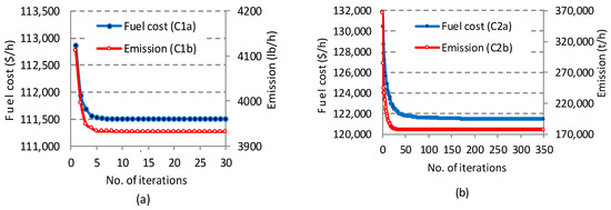
Figure 4.
Cost and emission convergence characteristics obtained using MSGO: (a) for cases C1a–C1b; (b) for cases C2a–C2b.
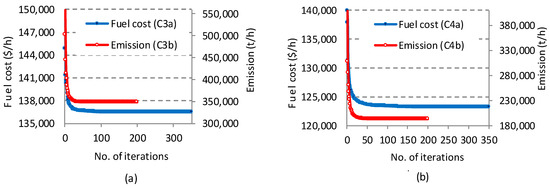
Figure 5.
Cost and emission convergence characteristics obtained using MSGO: (a) for cases C3a–C3b; (b) for cases C4a–C4b.
In the case of emission convergence characteristics (C1b–C4b), the iterative process stabilizes much faster than in the case of cost characteristics (C1a–C4a). Thus, in the case of the EmD problem (C1b–C4b), the quasi-stable process starts after about 20–30% of the maximum number of iterations, and in the EcD problem after approximately 40–50% of the maximum number of iterations. We mention that the stable values towards which the convergence characteristics of the MSGO algorithm tend are mentioned for each case in Table 5, Table 6, Table 7, Table 8, Table 9, Table 10, Table 11 and Table 12.
The accuracy and computation time: The accuracy (∆P) of the computations refers to the inequality and equality constraints of the optimization model presented in Section 2 and can be seen for the best solutions presented in Table 2, Table 3 and Table 4. It is observed that the constraints are respected, the size of ∆P being less than 10−5 MW for all cases studied. Also, for each case (C1a–C4a and C1b–C4b), the average execution time (Time) obtained using the MSGO algorithm is indicated in Table 2, Table 3 and Table 4. In cases C1a and C1b, the execution time is very good (under 0.2 s); for cases C2a and C2b it is higher (under 10 s) due to the larger size of the analyzed system (40-unit). In the cases C3a–C4a and C3b–C4b, due to the large size of the analyzed systems (40-unit) and the need to calculate power losses, the average execution time goes up to 33 s.
5.3. Results for EED Problem (Cases C1c–C4c)
The EED problem considers the cases C1c–C4c, in which the single-objective function Ф defined by relation (20) is minimized. In these cases, it is of interest to determine the Pareto front solutions, as well as the best compromise solution (BCS) obtained using the SGO and MSGO algorithms.
To estimate the Pareto front, the weighting factor ω in relation (20) is varied between 0 and 1 with a step of 0.1 (in the end 11 points are obtained in the Cost–Emission objective plan). However, in order to obtain a Pareto front as uniform as possible and to show graphically that the solutions obtained using MSGO dominate the solutions obtained using other algorithms, another 12 points have been added to the 11 points for the case C1c (the added points correspond to the values ω = {0.25, 0.35, 0.41, 0.42, 0.43, 0.435, 0.436, 0.44, 0.441, 0.445, 0.47, 0.55}) and 3 another points in the case of C2c (ω = {0.51, 0.52, 0.55}), respectively. In the case of C3c and C4c, the number of points considered is 11.
Figure 6, Figure 7 and Figure 8 show the Pareto fronts obtained using the SGO and MSGO algorithms for the cases C1c–C4c. Also, the best compromise solutions obtained using SGO, MSGO, and other competing algorithms applied in the literature are indicated.
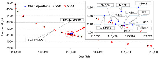
Figure 6.
Pareto fronts and BCSs obtained using SGO, MSGO, and other algorithms for case C1c.
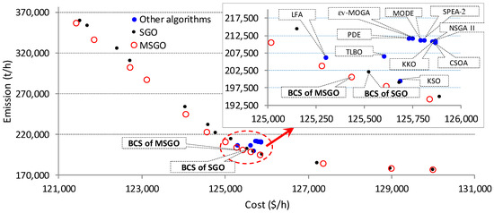
Figure 7.
Pareto fronts and BCSs obtained using SGO and MSGO for case C2c.
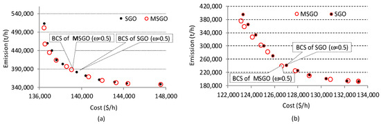
Figure 8.
Pareto fronts and BCSs obtained using SGO and MSGO: (a) for case C3c; (b) for case C4c.
Best compromise solution by SGO and MSGO: The BCSs obtained using the SGO and MSGO algorithms are identified using a fuzzy-based mechanism presented in Section 2.3. The results obtained through this mechanism indicate that BCS corresponds to a weighting factor equal to ω = 0.5, both for SGO and MSGO.
As a result, in Table 14, we present for each case C1c–C4c, the values for Cost, Emission, and item μmax (determined according to the methodology in Section 2.3) corresponding to the best compromise solution determined by SGO and MSGO.
Table 14.
The values corresponding to cost and emission obtained using SGO and MSGO for the cases C1c–C4c.
Comparison of solutions from the Pareto front of MSGO with BCSs obtained using other algorithms: In the case of C1c, in order to test the ability of MSGO to identify solutions from the Pareto front, it was compared with BCSs obtained using a group of algorithms (denoted G1) presented in the literature G1 = {EMOCA [24], MODE [42], NSGA II [42], TLBO [26], GSA [70], PDE [42], SMA [71], εv-MOGA [49], SPES-2 [42]}. To highlight the Pareto front solutions obtained using MSGO and BCSs obtained using competing algorithms in the G1 group, in Figure 6, a detail of the Cost–Emission plan is shown. In this detail of Figure 6, it can be visually observed that the Pareto front solutions obtained using MSGO (marked with red circles) dominate, in terms of Cost and Emission, all BCSs obtained using competing algorithms G1 (marked with blue circles). Thus, the points marked with red circles (obtained using MSGO) will remove from the Pareto front of MSGO all the points marked by blue circles (obtained using competing G1 algorithms). The exception is the IKSO algorithm [72], which obtains a non-dominated solution using the solutions in the Pareto front of the MSGO (a discussion on IKSO [72] will be made below).
In case of C2c, in Figure 7, a detail of the Cost–Emission plan is shown highlighting the Pareto front solutions obtained using MSGO, and BCSs obtained through several algorithms presented in the literature, denoted G2, G2 = {LFA [16], MODE [42], SPEA-2 [42], εv-MOGA [49], PDE [42], NSGA II [22], TLBO [26], CSOA [20], KKO [21], KSO [22]}. From the image it can be visually observed that the Pareto front solutions obtained using MSGO (marked with red circles) dominate, in terms of Cost and Emission, the BCSs obtained using the G2 group algorithms (marked with blue circles).
Comparison of BCSs obtained using MSGO and SGO: To compare BCSs obtained using the SGO and MSGO algorithms, we will include in the Pareto front of MSGO the best compromise solution identified for the SGO algorithm. Similarly, in the case of C1c, the BCS identified using the IKSO algorithm [72] will be included in the Pareto front of MSGO. Note that BCSs obtained using the SGO algorithm (cases C1c–C4c) or IKSO [72] (in the case of C1c) must be non-dominated solutions in the MSGO Pareto front. Thus, MSGO will have a Pareto front increased by one value (in cases C3c, corresponding to the BCS of SGO), respectively by two values (in cases C1c, corresponding to the BCSs of SGO and IKSO [72]). In cases C2c and C4c, the BCS of MSGO dominates the BCS of SGO in terms of Cost and Emission (see Table 14). The values from these extended Pareto fronts (with one or two other values) are subject to the methodology for establishing the BCS presented in Section 2.3, and the results of interest are given in Table 15. Table 15 shows the values of the item μmax obtained using the SGO, MSGO, and IKSO algorithms (we specify that the IKSO algorithm [72] is used only in the case of C1c). From Table 15, it can be seen that, for the cases C1c and C3c, the maximum value of the item μ corresponds to the MSGO algorithm (the weighting factor being for each case ω = 0.5). As a result, in all cases (C1c–C4c), the MSGO algorithm can identify a better compromise solution than SGO. Figure 5, Figure 6, Figure 7 and Figure 8 show the Pareto fronts obtained using SGO and MSGO and indicate the BCSs identified using these algorithms.
Table 15.
Values of item μmax obtained using SGO, MSGO and IKSO for cases C1c–C4c.
Comparison of SGO and MSGO Pareto fronts: Two metrics are used to evaluate and compare the quality of the Pareto fronts obtained using the SGO and MSGO algorithms: C-metric [73] and hyper-volume [74]. The C-metric, denoted C(S1, S2) and applied to the non-dominated solution sets S1 and S2, indicates the percentage of solutions from the S2 set dominated by the solutions from S1. For example, if C(S1, S2) = 100%, all solutions in S2 are dominated by those in S1. Currently, C(S1, S2) ≠ C(S2, S1) is required to calculate both metrics C(S1, S2) and C(S2, S1). The hyper-volume metric measures the volume (area in the case of two objectives) that is dominated by the Pareto front and is located below a predetermined reference point. Typically, higher values of the hyper-volume metric are associated with a better-quality Pareto front.
Table 16 shows, for each case, the values of the C-metric and hyper-volume metrics corresponding to the solution sets obtained using the SGO and MSGO algorithms. From Table 16 it can be seen that the C-metric (SGO, MSGO) = 0, which indicates that the solutions in the Pareto front obtained using SGO do not dominate any solution in the Pareto front obtained using the MSGO algorithm. Instead, the inverse C-metric (MSGO, SGO) indicates the percentages of SGO solutions dominated by MSGO solutions. Also, the hyper-volume metric shows higher values in the case of MSGO compared to SGO. Considering the values obtained using the two metrics, we estimate that MSGO can obtain a Pareto front of better quality than SGO.
Table 16.
Values of the metrics for assessing the Pareto fronts of SGO and MSGO.
When analyzing Table 4 from the EED problem point of view—case C4c—it shows that the BCS is obtained when the wind units operate at maximum capacity (PW1 ≈ PW2 ≈ 550 MW). When comparing the BCS-including wind (case C4c) with the BCS-without wind (case C3c), it results in lower costs (by 8.9%) and emissions (by 38.3%) for case C4c. Table 14 shows Cost savings and Emission reduction by MSGO compared to SGO for BCSs obtained in cases C1c–C4c. Positive values indicate that MSGO achieves better cost or lower emissions than SGO, and negative values indicate the opposite situation.
6. Conclusions
In this article, a modified SGO is proposed in which several terms in the solution update relations are disturbed by including chaotic sequences generated by the Logistic map and sequences generated by the HDP operator. Also, switching between solution update relations (in the acquiring phase) is achieved by introducing a random condition instead of a condition based on the value of the fitness function of the competing solutions. MSGO has been successfully tested for solving EcD, EmD, and EED problems for medium and large power systems.
The effectiveness of MSGO was tested on four cases for each type of problem (EcD, EmD, and EED). For all case studies targeting EcD, and EmD problems, MSGO obtained solutions of better or equal quality than well-known algorithms (such as: DE, ABC, PSO, SCA, etc.) or improved varieties (except for the cases mentioned in Section 5.2). Also, the convergence process was fast and the stability of the MSGO algorithm evaluated by the SD item was very good in cases C1b–C4b and relatively good in the cases C1a–C4a. The statistical items (B, A, W and SD) and the results of the Wilcoxon test show that MSGO is more efficient than SGO in six cases (out of a possible eight) and equally good in two cases (C2b and C3b in Table 13), indicating that the changes made in MSGO had a positive effect. In the case of the EED problem, MSGO was able to extract a better compromise solution than SGO or other algorithms for all studied cases C1c–C4c. Moreover, the values of the hyper-volume and C-metric indicate that MSGO can obtain a Pareto front of superior quality compared to SGO. It should be mentioned that the inclusion of wind sources (in the case of C4a/C4b compared to C3a/C3b) brings benefits both in terms of cost reduction (about 10%) and polluting emissions (about 45%). The average computation time of MSGO and SGO algorithms is similar, and the efficiency of both algorithms is good in all case studies. By applying economic and/or emissions dispatching using MSGO, electricity producers can make informed decisions to operate a sustainable energy system.
Author Contributions
Conceptualization, D.C.S., C.H. and M.L.S.; software data curation, D.C.S.; investigation, D.C.S., C.H., M.L.S., G.B., C.B. and F.C.D.; writing—original draft preparation, D.C.S., M.L.S. and C.B.; writing—review and editing, C.H., G.B., C.B. and F.C.D. All authors have read and agreed to the published version of the manuscript.
Funding
This research was funded by the University of Oradea within the framework of the grant competition “Scientific Research of Excellence Related to Priority Areas with Capitalization through Technology Transfer: INO-TRANSFER-UO-2nd Edition” projects no. 239/2022 and no. 236/2022.
Institutional Review Board Statement
Not applicable.
Informed Consent Statement
Not applicable.
Data Availability Statement
Data are contained within the article.
Acknowledgments
The research undertaken was made possible by the equal scientific involvement of all the authors concerned.
Conflicts of Interest
The authors declare no conflicts of interest.
Nomenclature
| ai, bi, ci, ei, and fi | Fuel cost coefficients of thermal unit i; |
| Bij, B0i, B00 | Loss coefficients; |
| c | Self-introspection parameter from SGO; |
| Direct, reserve, and penalty cost coefficient for unit j; | |
| C(PT,PW) | Total fuel cost; |
| Reserve, and penalty emission coefficient for unit j; | |
| , | Mean powers associated with over and underestimation Wj for unit j; |
| E(PT,PW) | Total emission; |
| f(Xbest) | Objective function associated to Xbest; |
| fi = f(Xi), f(Xr) | Objective function associated to Xi and Xr solutions; |
| k, c | Shape, and scale parameters of Weibull distribution; |
| n | Problem dimension; |
| N | Population size; |
| Nt, Nw | The number of thermal and wind units; |
| o, u | Superscript symbols attached to some quantities reflecting overestimation, and underestimation of the available wind power; |
| PD | The total power demand; |
| PL | Transmission line losses; |
| PT, PW | The output power vectors of the thermal and wind units; |
| PTi | Power of the thermal unit i; |
| PTmin,i, PTmax,i | Real minimum and maximum power of the thermal unit i; |
| PWj | Scheduled wind power of the wind unit j; |
| PWr | Rated power of the wind unit; |
| ru, δ | Parameters specific to the HDP operator; |
| t | Current iteration; |
| tmax | Maximum number of iterations |
| vin, vr, vout | Cut-in, rated, and cut-out wind speeds of the wind unit; |
| Wj | Random variable that represents available wind power for unit j; |
| Xi, Xr | n-dimensional vectors associated with solutions i and r; |
| New solution vector Xi; | |
| Xbest | The vector of the best solution; |
| xj,i | jth component of solution Xi; |
| jth component of solution | |
| jth component of solution Xbest | |
| α, β, δmax | Specific parameters of the MSGO algorithm; |
| αj, βj, γj, δj, and λj | Emission coefficients of the thermal unit i; |
| ω | Weighting factor; |
| {cxp} | Chaotic sequence; |
| exp(•) | exponential function; |
| fW(•) | Probability density function (pdf) of random variable W; |
| Prob(•) | The probability of the event; |
| min, max | Indicate the minimum and maximum limits of some variables/functions; |
| Min, Max | Mathematical functions that determine the minimum and maximum value in a set. |
Abbreviations
ABC: Artificial bee colony algorithm; ACS: Artificial cooperative search; BBO: Biogeography-based optimization; BCS: Best compromise solution; BSA: Backtracking search optimization; CA: Cultural algorithm; CSCA: Chaotic SCA; CSO: Cuckoo search optimization; CSOA: Criminal search optimization algorithm; CSS: Charged system search; CTLBO: Chaotic TLBO; CTO: Class topper optimization; DE: Differential evolution; EcD: Economic dispatch; EED: Economic emission dispatch; EmD: Emission dispatch; EMA: Exchange market algorithm; EMOCA: Enhanced multi-objective cultural algorithm; εv-MOGA: Epsilon-multi-objective GA; ESCSDO10: Eagle-strategy supply–demand based optimization algorithm with chaotic map ten; FSS-IPSO2: Floating search space with improved PSO; GA: Genetic algorithm; GAAPI: GA with ant colony optimization; GQPSO: Gaussian quantum-behaved PSO; GSA: Gravitational search algorithm; GWO: Grey wolf optimization; HDP: Highly disruptive polynomial; HPSO-DE: Hybrid PSO with DE; HSCA: Hybrid SCA; IJaya: Improved Jaya algorithm; IKSO: Improve kernel search optimization; IMO: Ion motion optimization; ISA: Interior search algorithm; Jaya-SML: Jaya algorithm with SAMP and Lévy flights; KKO: Kho-Kho optimization algorithm; KSO: Kernel search optimization; LFA: Lightning flash algorithm; LPSR: Linear population size reduction; L-SHADE: LPSR with success-history based adaptive DE; MBFA: Modified bacterial foraging algorithm; MIMO: Modified IMO; MODE: Multi-objective DE; MSGO: Modified SGO; NGWO: Novel grey wolf optimization; NSGA II/III: Non-dominated sorting genetic algorithm-version II/III; ORCCRO: Oppositional real coded chemical reaction optimization; PDE: Pareto differential evolution; pdf: Probability density function; PSO: Particle swarm optimization; QOPO: Quasi-oppositional-based political optimizer; QOTLBO: Quasi-oppositional TLBO; QPSO: Quantum PSO; RCCRO: Real coded chemical reaction optimization; SAMP: Self-adaptive multi-population; SCA: Sine–cosine algorithm; SDE: Shuffled differential evolution; SDO: Supply–demand optimization; SGO: Social group optimization; S-Jaya: Jaya with self-adaptive po-pulation mechanism; SMA: Slime mould algorithm; SPES-2: Strength pareto evolutionary algorithm 2; SSA: Squirrel search algorithm; TLABC: Teaching-learning-based ABC; TLBO: Teaching learning-based-optimization; VPE: Valve-point effects; Wind: Indicates the inclusion of wind power in EcD, EmD, or EED problems.
Appendix A
Table A1.
Assessment of the cost related to wind power: steps and numerical example.
Table A1.
Assessment of the cost related to wind power: steps and numerical example.
| Step | Description and Exemplification |
|---|---|
| To Evaluate the Cost Related to the Wind Power, the Main Steps That Have to Be Done Are Presented, as Well as How Each of Them Is Applied for a Specific Case of a Wind Unit: | |
| 1 | Set the input data for a wind unit: the shape (k = 1.5) and scale (c = 15) parameters; rated output power of the wind unit (PWr = 550 MW); cut-in wind speed (vin = 5 m/s), rated wind speed (vr = 15 m/s), cut-out wind speed (vout = 45 m/s); direct cost coefficient (cd = 0), reserve cost coefficient (co = 5), penalty cost coefficient (cu = 5). Because during the MSGO optimization process, the variable “scheduled wind power” (PW) vary between the limits (PWmin = 0, PWmax = 550) MW, the calculation is performed for an arbitrarily chosen value, for example PW = 400 MW |
| 2 | Set the expression of the pdf fW(w) related to the wind power (W) using relation (7): |
| 3 | Calculate the discrete probabilities Prob(W = 0), and Prob(W = PWr), using relations (8) and (9): Prob(W = 0) = 1 − exp[−(vin/c)k] + exp[−(vout/c)k] = 1 − exp[(−(5/15)1.5] + exp[−(45/15)1.5] = 0.180602 Prob(W = PWr) = Prob(W = 550) = exp[−(vr/c)k] − exp[−(vout/c)k] = exp[−(15/15)1.5] − exp[−(45/15)1.5] = 0.362342 |
| 4 | Calculate the average power (PW = 400) and (PW = 400) according to (10) and (11): where fW(w) is presented in Step 2 and the integrals may by directly calculated in mathcad. |
| 5 | Calculate the cost CW(PW) related to the wind power PW, using (3): |
Table A2.
Thermal units’ characteristics for the 10-unit test system.
Table A2.
Thermal units’ characteristics for the 10-unit test system.
| Unit | Power Limits | Fuel Cost Coefficients | Emission Coefficients | |||||||||
|---|---|---|---|---|---|---|---|---|---|---|---|---|
| Pmin,i | Pmax,i | ai | bi | ci | ei | fi | αi | βi | γi | δi | λi | |
| MW | MW | $/MW2h | $/MWh | $/h | $/h | rad/MW | lb/MW2h | lb/MWh | lb/h | lb/h | 1/MW | |
| 1 | 10 | 55 | 0.12951 | 40.5407 | 1000.403 | 33 | 0.0174 | 0.04702 | −3.9864 | 360.0012 | 0.25475 | 0.01234 |
| 2 | 20 | 80 | 0.10908 | 39.5804 | 950.606 | 25 | 0.0178 | 0.04652 | −3.9524 | 350.0056 | 0.25475 | 0.01234 |
| 3 | 47 | 120 | 0.12511 | 36.5104 | 900.705 | 32 | 0.0162 | 0.04652 | −3.9023 | 330.0056 | 0.25163 | 0.01215 |
| 4 | 20 | 130 | 0.12111 | 39.5104 | 800.705 | 30 | 0.0168 | 0.04652 | −3.9023 | 330.0056 | 0.25163 | 0.01215 |
| 5 | 50 | 160 | 0.15247 | 38.5390 | 756.799 | 30 | 0.0148 | 0.00420 | 0.3277 | 13.8593 | 0.24970 | 0.01200 |
| 6 | 70 | 240 | 0.10587 | 46.1592 | 451.325 | 20 | 0.0163 | 0.00420 | 0.3277 | 13.8593 | 0.24970 | 0.01200 |
| 7 | 60 | 300 | 0.03546 | 38.3055 | 1243.531 | 20 | 0.0152 | 0.00680 | −0.5455 | 40.2669 | 0.24800 | 0.01290 |
| 8 | 70 | 340 | 0.02803 | 40.3965 | 1049.998 | 30 | 0.0128 | 0.00680 | −0.5455 | 40.2669 | 0.24990 | 0.01203 |
| 9 | 135 | 470 | 0.02111 | 36.3278 | 1658.569 | 60 | 0.0136 | 0.00460 | −0.5112 | 42.8955 | 0.25470 | 0.01234 |
| 10 | 150 | 470 | 0.01799 | 38.2704 | 1356.659 | 40 | 0.0141 | 0.00460 | −0.5112 | 42.8955 | 0.25470 | 0.01234 |
Table A3.
The B-loss coefficients ([Bij], [B0i], and B00) for 10-unit system.
Table A3.
The B-loss coefficients ([Bij], [B0i], and B00) for 10-unit system.
| 1 | 2 | 3 | 4 | 5 | 6 | 7 | 8 | 9 | 10 | ||
|---|---|---|---|---|---|---|---|---|---|---|---|
| 1 | 4.9 × 10⁻⁵ | 1.4 × 10⁻⁵ | 1.5 × 10⁻⁵ | 1.5 × 10⁻⁵ | 1.6 × 10⁻⁵ | 1.7 × 10⁻⁵ | 1.7 × 10⁻⁵ | 1.8 × 10⁻⁵ | 1.9 × 10⁻⁵ | 2.0 × 10⁻⁵ | |
| 2 | 1.4 × 10⁻⁵ | 4.5 × 10⁻⁵ | 1.6 × 10⁻⁵ | 1.6 × 10⁻⁵ | 1.7 × 10⁻⁵ | 1.5 × 10⁻⁵ | 1.5 × 10⁻⁵ | 1.6 × 10⁻⁵ | 1.8 × 10⁻⁵ | 1.8 × 10⁻⁵ | |
| 3 | 1.5 × 10⁻⁵ | 1.6 × 10⁻⁵ | 3.9 × 10⁻⁵ | 1.0 × 10⁻⁵ | 1.2 × 10⁻⁵ | 1.2 × 10⁻⁵ | 1.4 × 10⁻⁵ | 1.4 × 10⁻⁵ | 1.6 × 10⁻⁵ | 1.6 × 10⁻⁵ | |
| 4 | 1.5 × 10⁻⁵ | 1.6 × 10⁻⁵ | 1.0 × 10⁻⁵ | 4.0 × 10⁻⁵ | 1.4 × 10⁻⁵ | 1.0 × 10⁻⁵ | 1.1 × 10⁻⁵ | 1.2 × 10⁻⁵ | 1.4 × 10⁻⁵ | 1.5 × 10⁻⁵ | |
| [Bij]10×10= | 5 | 1.6 × 10⁻⁵ | 1.7 × 10⁻⁵ | 1.2 × 10⁻⁵ | 1.4 × 10⁻⁵ | 3.5 × 10⁻⁵ | 1.1 × 10⁻⁵ | 1.3 × 10⁻⁵ | 1.3 × 10⁻⁵ | 1.5 × 10⁻⁵ | 1.6 × 10⁻⁵ |
| 6 | 1.7 × 10⁻⁵ | 1.5 × 10⁻⁵ | 1.2 × 10⁻⁵ | 1.0 × 10⁻⁵ | 1.1 × 10⁻⁵ | 3.6 × 10⁻⁵ | 1.2 × 10⁻⁵ | 1.2 × 10⁻⁵ | 1.4 × 10⁻⁵ | 1.5 × 10⁻⁵ | |
| 7 | 1.7 × 10⁻⁵ | 1.5 × 10⁻⁵ | 1.4 × 10⁻⁵ | 1.1 × 10⁻⁵ | 1.3 × 10⁻⁵ | 1.2 × 10⁻⁵ | 3.8 × 10⁻⁵ | 1.6 × 10⁻⁵ | 1.6 × 10⁻⁵ | 1.8 × 10⁻⁵ | |
| 8 | 1.8 × 10⁻⁵ | 1.6 × 10⁻⁵ | 1.4 × 10⁻⁵ | 1.2 × 10⁻⁵ | 1.3 × 10⁻⁵ | 1.2 × 10⁻⁵ | 1.6 × 10⁻⁵ | 4.0 × 10⁻⁵ | 1.5 × 10⁻⁵ | 1.6 × 10⁻⁵ | |
| 9 | 1.9 × 10⁻⁵ | 1.8 × 10⁻⁵ | 1.6 × 10⁻⁵ | 1.4 × 10⁻⁵ | 1.5 × 10⁻⁵ | 1.4 × 10⁻⁵ | 1.6 × 10⁻⁵ | 1.5 × 10⁻⁵ | 4.2 × 10⁻⁵ | 1.9 × 10⁻⁵ | |
| 10 | 2.0 × 10⁻⁵ | 1.8 × 10⁻⁵ | 1.6 × 10⁻⁵ | 1.5 × 10⁻⁵ | 1.6 × 10⁻⁵ | 1.5 × 10⁻⁵ | 1.8 × 10⁻⁵ | 1.6 × 10⁻⁵ | 1.9 × 10⁻⁵ | 4.4 × 10⁻⁵ | |
| [B0i]1×10= | 0 | 0 | 0 | 0 | 0 | 0 | 0 | 0 | 0 | 0 | |
| B00= | 0 |
Table A4.
Thermal units’ characteristics for the 40-unit test system.
Table A4.
Thermal units’ characteristics for the 40-unit test system.
| Unit | Power Limits | Fuel Cost Coefficients | Emission Coefficients | |||||||||
|---|---|---|---|---|---|---|---|---|---|---|---|---|
| Pmin,i | Pmax,i | ai | bi | ci | ei | fi | αi | βi | γi | δi | λi | |
| MW | MW | $/MW2h | $/MWh | $/h | $/h | rad/MW | t/MW2h | t/MWh | t/h | t/h | 1/MW | |
| 1 | 36 | 114 | 0.0069 | 6.73 | 94.705 | 100 | 0.084 | 0.048 | −2.22 | 60 | 1.31 | 0.0569 |
| 2 | 36 | 114 | 0.0069 | 6.73 | 94.705 | 100 | 0.084 | 0.048 | −2.22 | 60 | 1.31 | 0.0569 |
| 3 | 60 | 120 | 0.02028 | 7.07 | 309.54 | 100 | 0.084 | 0.0762 | −2.36 | 100 | 1.31 | 0.0569 |
| 4 | 80 | 190 | 0.00942 | 8.18 | 369.03 | 150 | 0.063 | 0.054 | −3.14 | 120 | 0.9142 | 0.0454 |
| 5 | 47 | 97 | 0.0114 | 5.35 | 148.89 | 120 | 0.077 | 0.085 | −1.89 | 50 | 0.9936 | 0.0406 |
| 6 | 68 | 140 | 0.01142 | 8.05 | 222.33 | 100 | 0.084 | 0.0854 | −3.08 | 80 | 1.31 | 0.0569 |
| 7 | 110 | 300 | 0.00357 | 8.03 | 287.71 | 200 | 0.042 | 0.0242 | −3.06 | 100 | 0.6550 | 0.02846 |
| 8 | 135 | 300 | 0.00492 | 6.99 | 391.98 | 200 | 0.042 | 0.031 | −2.32 | 130 | 0.6550 | 0.02846 |
| 9 | 135 | 300 | 0.00573 | 6.6 | 455.76 | 200 | 0.042 | 0.0335 | −2.11 | 150 | 0.6550 | 0.02846 |
| 10 | 130 | 300 | 0.00605 | 12.9 | 722.82 | 200 | 0.042 | 0.425 | −4.34 | 280 | 0.6550 | 0.02846 |
| 11 | 94 | 375 | 0.00515 | 12.9 | 635.2 | 200 | 0.042 | 0.0322 | −4.34 | 220 | 0.6550 | 0.02846 |
| 12 | 94 | 375 | 0.00569 | 12.8 | 654.69 | 200 | 0.042 | 0.0338 | −4.28 | 225 | 0.6550 | 0.02846 |
| 13 | 125 | 500 | 0.00421 | 12.5 | 913.4 | 300 | 0.035 | 0.0296 | −4.18 | 300 | 0.5035 | 0.02075 |
| 14 | 125 | 500 | 0.00752 | 8.84 | 1760.4 | 300 | 0.035 | 0.0512 | −3.34 | 520 | 0.5035 | 0.02075 |
| 15 | 125 | 500 | 0.00708 | 9.15 | 1728.3 | 300 | 0.035 | 0.0496 | −3.55 | 510 | 0.5035 | 0.02075 |
| 16 | 125 | 500 | 0.00708 | 9.15 | 1728.3 | 300 | 0.035 | 0.0496 | −3.55 | 510 | 0.5035 | 0.02075 |
| 17 | 220 | 500 | 0.00313 | 7.97 | 647.85 | 300 | 0.035 | 0.0151 | −2.68 | 220 | 0.5035 | 0.02075 |
| 18 | 220 | 500 | 0.00313 | 7.95 | 649.69 | 300 | 0.035 | 0.0151 | −2.66 | 222 | 0.5035 | 0.02075 |
| 19 | 242 | 550 | 0.00313 | 7.97 | 647.83 | 300 | 0.035 | 0.0151 | −2.68 | 220 | 0.5035 | 0.02075 |
| 20 | 242 | 550 | 0.00313 | 7.97 | 647.81 | 300 | 0.035 | 0.0151 | −2.68 | 220 | 0.5035 | 0.02075 |
| 21 | 254 | 550 | 0.00298 | 6.63 | 785.96 | 300 | 0.035 | 0.0145 | −2.22 | 290 | 0.5035 | 0.02075 |
| 22 | 254 | 550 | 0.00298 | 6.63 | 785.96 | 300 | 0.035 | 0.0145 | −2.22 | 285 | 0.5035 | 0.02075 |
| 23 | 254 | 550 | 0.00284 | 6.66 | 794.53 | 300 | 0.035 | 0.0138 | −2.26 | 295 | 0.5035 | 0.02075 |
| 24 | 254 | 550 | 0.00284 | 6.66 | 794.53 | 300 | 0.035 | 0.0138 | −2.26 | 295 | 0.5035 | 0.02075 |
| 25 | 254 | 550 | 0.00277 | 7.1 | 801.32 | 300 | 0.035 | 0.0132 | −2.42 | 310 | 0.5035 | 0.02075 |
| 26 | 254 | 550 | 0.00277 | 7.1 | 801.32 | 300 | 0.035 | 0.0132 | −2.42 | 310 | 0.5035 | 0.02075 |
| 27 | 10 | 150 | 0.52124 | 3.33 | 1055.1 | 120 | 0.077 | 1.842 | −1.11 | 360 | 0.9936 | 0.0406 |
| 28 | 10 | 150 | 0.52124 | 3.33 | 1055.1 | 120 | 0.077 | 1.842 | −1.11 | 360 | 0.9936 | 0.0406 |
| 29 | 10 | 150 | 0.52124 | 3.33 | 1055.1 | 120 | 0.077 | 1.842 | −1.11 | 360 | 0.9936 | 0.0406 |
| 30 | 47 | 97 | 0.0114 | 5.35 | 148.89 | 120 | 0.077 | 0.085 | −1.89 | 50 | 0.9936 | 0.0406 |
| 31 | 60 | 190 | 0.0016 | 6.43 | 222.92 | 150 | 0.063 | 0.0121 | −2.08 | 80 | 0.9142 | 0.0454 |
| 32 | 60 | 190 | 0.0016 | 6.43 | 222.92 | 150 | 0.063 | 0.0121 | −2.08 | 80 | 0.9142 | 0.0454 |
| 33 | 60 | 190 | 0.0016 | 6.43 | 222.92 | 150 | 0.063 | 0.0121 | −2.08 | 80 | 0.9142 | 0.0454 |
| 34 | 90 | 200 | 0.0001 | 8.95 | 107.87 | 200 | 0.042 | 0.0012 | −3.48 | 65 | 0.6550 | 0.02846 |
| 35 | 90 | 200 | 0.0001 | 8.62 | 116.58 | 200 | 0.042 | 0.0012 | −3.24 | 70 | 0.6550 | 0.02846 |
| 36 | 90 | 200 | 0.0001 | 8.62 | 116.58 | 200 | 0.042 | 0.0012 | −3.24 | 70 | 0.6550 | 0.02846 |
| 37 | 25 | 110 | 0.0161 | 5.88 | 307.45 | 80 | 0.098 | 0.095 | −1.98 | 100 | 1.42 | 0.0677 |
| 38 | 25 | 110 | 0.0161 | 5.88 | 307.45 | 80 | 0.098 | 0.095 | −1.98 | 100 | 1.42 | 0.0677 |
| 39 | 25 | 110 | 0.0161 | 5.88 | 307.45 | 80 | 0.098 | 0.095 | −1.98 | 100 | 1.42 | 0.0677 |
| 40 | 242 | 550 | 0.00313 | 7.97 | 647.83 | 300 | 0.035 | 0.0151 | −2.68 | 220 | 0.5035 | 0.02075 |
Table A5.
The B-loss coefficients ([Bij], [B0i], and B00) for 40-unit system.
Table A5.
The B-loss coefficients ([Bij], [B0i], and B00) for 40-unit system.
| ([Bij]40×40) × 10−6 = | 1 | 2 | 3 | 4 | 5 | 6 | 7 | 8 | 9 | 10 | 11 | 12 | 13 | 14 | 15 | 16 | 17 | 18 | 19 | 20 | 21 | 22 | 23 | 24 | 25 | 26 | 27 | 28 | 29 | 30 | 31 | 32 | 33 | 34 | 35 | 36 | 37 | 38 | 39 | 40 | |
| 1 | 17 | 12 | 7 | −1 | −5 | −2 | 17 | 12 | 7 | −1 | −5 | −2 | 17 | 12 | 7 | −1 | −5 | −2 | 17 | 12 | 7 | −1 | −5 | −2 | 17 | 12 | 7 | −1 | −5 | −2 | 17 | 12 | 7 | −1 | −5 | −2 | 17 | 12 | 7 | −1 | |
| 2 | 12 | 14 | 9 | 1 | −6 | −1 | 12 | 14 | 9 | 1 | −6 | −1 | 12 | 14 | 9 | 1 | −6 | −1 | 12 | 14 | 9 | 1 | −6 | −1 | 12 | 14 | 9 | 1 | −6 | −1 | 12 | 14 | 9 | 1 | −6 | −1 | 12 | 14 | 9 | 1 | |
| 3 | 7 | 9 | 31 | 0 | −10 | −6 | 7 | 9 | 31 | 0 | −10 | −6 | 7 | 9 | 31 | 0 | −10 | −6 | 7 | 9 | 31 | 0 | −10 | −6 | 7 | 9 | 31 | 0 | −10 | −6 | 7 | 9 | 31 | 0 | −10 | −6 | 7 | 9 | 31 | 0 | |
| 4 | −1 | 1 | 0 | 24 | −6 | −8 | −1 | 1 | 0 | 24 | −6 | −8 | −1 | 1 | 0 | 24 | −6 | −8 | −1 | 1 | 0 | 24 | −6 | −8 | −1 | 1 | 0 | 24 | −6 | −8 | −1 | 1 | 0 | 24 | −6 | −8 | −1 | 1 | 0 | 24 | |
| 5 | −5 | −6 | −10 | −6 | 129 | −2 | −5 | −6 | −10 | −6 | 129 | −2 | −5 | −6 | −10 | −6 | 129 | −2 | −5 | −6 | −10 | −6 | 129 | −2 | −5 | −6 | −10 | −6 | 129 | −2 | −5 | −6 | −10 | −6 | 129 | −2 | −5 | −6 | −10 | −6 | |
| 6 | −2 | −1 | −6 | −8 | −2 | 150 | −2 | −1 | −6 | −8 | −2 | 150 | −2 | −1 | −6 | −8 | −2 | 150 | −2 | −1 | −6 | −8 | −2 | 150 | −2 | −1 | −6 | −8 | −2 | 150 | −2 | −1 | −6 | −8 | −2 | 150 | −2 | −1 | −6 | −8 | |
| 7 | 17 | 12 | 7 | −1 | −5 | −2 | 17 | 12 | 7 | −1 | −5 | −2 | 17 | 12 | 7 | −1 | −5 | −2 | 17 | 12 | 7 | −1 | −5 | −2 | 17 | 12 | 7 | −1 | −5 | −2 | 17 | 12 | 7 | −1 | −5 | −2 | 17 | 12 | 7 | −1 | |
| 8 | 12 | 14 | 9 | 1 | −6 | −1 | 12 | 14 | 9 | 1 | −6 | −1 | 12 | 14 | 9 | 1 | −6 | −1 | 12 | 14 | 9 | 1 | −6 | −1 | 12 | 14 | 9 | 1 | −6 | −1 | 12 | 14 | 9 | 1 | −6 | −1 | 12 | 14 | 9 | 1 | |
| 9 | 7 | 9 | 31 | 0 | −10 | −6 | 7 | 9 | 31 | 0 | −10 | −6 | 7 | 9 | 31 | 0 | −10 | −6 | 7 | 9 | 31 | 0 | −10 | −6 | 7 | 9 | 31 | 0 | −10 | −6 | 7 | 9 | 31 | 0 | −10 | −6 | 7 | 9 | 31 | 0 | |
| 10 | −1 | 1 | 0 | 24 | −6 | −8 | −1 | 1 | 0 | 24 | −6 | −8 | −1 | 1 | 0 | 24 | −6 | −8 | −1 | 1 | 0 | 24 | −6 | −8 | −1 | 1 | 0 | 24 | −6 | −8 | −1 | 1 | 0 | 24 | −6 | −8 | −1 | 1 | 0 | 24 | |
| 11 | −5 | −6 | −10 | −6 | 129 | −2 | −5 | −6 | −10 | −6 | 129 | −2 | −5 | −6 | −10 | −6 | 129 | −2 | −5 | −6 | −10 | −6 | 129 | −2 | −5 | −6 | −10 | −6 | 129 | −2 | −5 | −6 | −10 | −6 | 129 | −2 | −5 | −6 | −10 | −6 | |
| 12 | −2 | −1 | −6 | −8 | −2 | 150 | −2 | −1 | −6 | −8 | −2 | 150 | −2 | −1 | −6 | −8 | −2 | 150 | −2 | −1 | −6 | −8 | −2 | 150 | −2 | −1 | −6 | −8 | −2 | 150 | −2 | −1 | −6 | −8 | −2 | 150 | −2 | −1 | −6 | −8 | |
| 13 | 17 | 12 | 7 | −1 | −5 | −2 | 17 | 12 | 7 | −1 | −5 | −2 | 17 | 12 | 7 | −1 | −5 | −2 | 17 | 12 | 7 | −1 | −5 | −2 | 17 | 12 | 7 | −1 | −5 | −2 | 17 | 12 | 7 | −1 | −5 | −2 | 17 | 12 | 7 | −1 | |
| 14 | 12 | 14 | 9 | 1 | −6 | −1 | 12 | 14 | 9 | 1 | −6 | −1 | 12 | 14 | 9 | 1 | −6 | −1 | 12 | 14 | 9 | 1 | −6 | −1 | 12 | 14 | 9 | 1 | −6 | −1 | 12 | 14 | 9 | 1 | −6 | −1 | 12 | 14 | 9 | 1 | |
| 15 | 7 | 9 | 31 | 0 | −10 | −6 | 7 | 9 | 31 | 0 | −10 | −6 | 7 | 9 | 31 | 0 | −10 | −6 | 7 | 9 | 31 | 0 | −10 | −6 | 7 | 9 | 31 | 0 | −10 | −6 | 7 | 9 | 31 | 0 | −10 | −6 | 7 | 9 | 31 | 0 | |
| 16 | −1 | 1 | 0 | 24 | −6 | −8 | −1 | 1 | 0 | 24 | −6 | −8 | −1 | 1 | 0 | 24 | −6 | −8 | −1 | 1 | 0 | 24 | −6 | −8 | −1 | 1 | 0 | 24 | −6 | −8 | −1 | 1 | 0 | 24 | −6 | −8 | −1 | 1 | 0 | 24 | |
| 17 | −5 | −6 | −10 | −6 | 129 | −2 | −5 | −6 | −10 | −6 | 129 | −2 | −5 | −6 | −10 | −6 | 129 | −2 | −5 | −6 | −10 | −6 | 129 | −2 | −5 | −6 | −10 | −6 | 129 | −2 | −5 | −6 | −10 | −6 | 129 | −2 | −5 | −6 | −10 | −6 | |
| 18 | −2 | −1 | −6 | −8 | −2 | 150 | −2 | −1 | −6 | −8 | −2 | 150 | −2 | −1 | −6 | −8 | −2 | 150 | −2 | −1 | −6 | −8 | −2 | 150 | −2 | −1 | −6 | −8 | −2 | 150 | −2 | −1 | −6 | −8 | −2 | 150 | −2 | −1 | −6 | −8 | |
| 19 | 17 | 12 | 7 | −1 | −5 | −2 | 17 | 12 | 7 | −1 | −5 | −2 | 17 | 12 | 7 | −1 | −5 | −2 | 17 | 12 | 7 | −1 | −5 | −2 | 17 | 12 | 7 | −1 | −5 | −2 | 17 | 12 | 7 | −1 | −5 | −2 | 17 | 12 | 7 | −1 | |
| 20 | 12 | 14 | 9 | 1 | −6 | −1 | 12 | 14 | 9 | 1 | −6 | −1 | 12 | 14 | 9 | 1 | −6 | −1 | 12 | 14 | 9 | 1 | −6 | −1 | 12 | 14 | 9 | 1 | −6 | −1 | 12 | 14 | 9 | 1 | −6 | −1 | 12 | 14 | 9 | 1 | |
| 21 | 7 | 9 | 31 | 0 | −10 | −6 | 7 | 9 | 31 | 0 | −10 | −6 | 7 | 9 | 31 | 0 | −10 | −6 | 7 | 9 | 31 | 0 | −10 | −6 | 7 | 9 | 31 | 0 | −10 | −6 | 7 | 9 | 31 | 0 | −10 | −6 | 7 | 9 | 31 | 0 | |
| 22 | −1 | 1 | 0 | 24 | −6 | −8 | −1 | 1 | 0 | 24 | −6 | −8 | −1 | 1 | 0 | 24 | −6 | −8 | −1 | 1 | 0 | 24 | −6 | −8 | −1 | 1 | 0 | 24 | −6 | −8 | −1 | 1 | 0 | 24 | −6 | −8 | −1 | 1 | 0 | 24 | |
| 23 | −5 | −6 | −10 | −6 | 129 | −2 | −5 | −6 | −10 | −6 | 129 | −2 | −5 | −6 | −10 | −6 | 129 | −2 | −5 | −6 | −10 | −6 | 129 | −2 | −5 | −6 | −10 | −6 | 129 | −2 | −5 | −6 | −10 | −6 | 129 | −2 | −5 | −6 | −10 | −6 | |
| 24 | −2 | −1 | −6 | −8 | −2 | 150 | −2 | −1 | −6 | −8 | −2 | 150 | −2 | −1 | −6 | −8 | −2 | 150 | −2 | −1 | −6 | −8 | −2 | 150 | −2 | −1 | −6 | −8 | −2 | 150 | −2 | −1 | −6 | −8 | −2 | 150 | −2 | −1 | −6 | −8 | |
| 25 | 17 | 12 | 7 | −1 | −5 | −2 | 17 | 12 | 7 | −1 | −5 | −2 | 17 | 12 | 7 | −1 | −5 | −2 | 17 | 12 | 7 | −1 | −5 | −2 | 17 | 12 | 7 | −1 | −5 | −2 | 17 | 12 | 7 | −1 | −5 | −2 | 17 | 12 | 7 | −1 | |
| 26 | 12 | 14 | 9 | 1 | −6 | −1 | 12 | 14 | 9 | 1 | −6 | −1 | 12 | 14 | 9 | 1 | −6 | −1 | 12 | 14 | 9 | 1 | −6 | −1 | 12 | 14 | 9 | 1 | −6 | −1 | 12 | 14 | 9 | 1 | −6 | −1 | 12 | 14 | 9 | 1 | |
| 27 | 7 | 9 | 31 | 0 | −10 | −6 | 7 | 9 | 31 | 0 | −10 | −6 | 7 | 9 | 31 | 0 | −10 | −6 | 7 | 9 | 31 | 0 | −10 | −6 | 7 | 9 | 31 | 0 | −10 | −6 | 7 | 9 | 31 | 0 | −10 | −6 | 7 | 9 | 31 | 0 | |
| 28 | −1 | 1 | 0 | 24 | −6 | −8 | −1 | 1 | 0 | 24 | −6 | −8 | −1 | 1 | 0 | 24 | −6 | −8 | −1 | 1 | 0 | 24 | −6 | −8 | −1 | 1 | 0 | 24 | −6 | −8 | −1 | 1 | 0 | 24 | −6 | −8 | −1 | 1 | 0 | 24 | |
| 29 | −5 | −6 | −10 | −6 | 129 | −2 | −5 | −6 | −10 | −6 | 129 | −2 | −5 | −6 | −10 | −6 | 129 | −2 | −5 | −6 | −10 | −6 | 129 | −2 | −5 | −6 | −10 | −6 | 129 | −2 | −5 | −6 | −10 | −6 | 129 | −2 | −5 | −6 | −10 | −6 | |
| 30 | −2 | −1 | −6 | −8 | −2 | 150 | −2 | −1 | −6 | −8 | −2 | 150 | −2 | −1 | −6 | −8 | −2 | 150 | −2 | −1 | −6 | −8 | −2 | 150 | −2 | −1 | −6 | −8 | −2 | 150 | −2 | −1 | −6 | −8 | −2 | 150 | −2 | −1 | −6 | −8 | |
| 31 | 17 | 12 | 7 | −1 | −5 | −2 | 17 | 12 | 7 | −1 | −5 | −2 | 17 | 12 | 7 | −1 | −5 | −2 | 17 | 12 | 7 | −1 | −5 | −2 | 17 | 12 | 7 | −1 | −5 | −2 | 17 | 12 | 7 | −1 | −5 | −2 | 17 | 12 | 7 | −1 | |
| 32 | 12 | 14 | 9 | 1 | −6 | −1 | 12 | 14 | 9 | 1 | −6 | −1 | 12 | 14 | 9 | 1 | −6 | −1 | 12 | 14 | 9 | 1 | −6 | −1 | 12 | 14 | 9 | 1 | −6 | −1 | 12 | 14 | 9 | 1 | −6 | −1 | 12 | 14 | 9 | 1 | |
| 33 | 7 | 9 | 31 | 0 | −10 | −6 | 7 | 9 | 31 | 0 | −10 | −6 | 7 | 9 | 31 | 0 | −10 | −6 | 7 | 9 | 31 | 0 | −10 | −6 | 7 | 9 | 31 | 0 | −10 | −6 | 7 | 9 | 31 | 0 | −10 | −6 | 7 | 9 | 31 | 0 | |
| 34 | −1 | 1 | 0 | 24 | −6 | −8 | −1 | 1 | 0 | 24 | −6 | −8 | −1 | 1 | 0 | 24 | −6 | −8 | −1 | 1 | 0 | 24 | −6 | −8 | −1 | 1 | 0 | 24 | −6 | −8 | −1 | 1 | 0 | 24 | −6 | −8 | −1 | 1 | 0 | 24 | |
| 35 | −5 | −6 | −10 | −6 | 129 | −2 | −5 | −6 | −10 | −6 | 129 | −2 | −5 | −6 | −10 | −6 | 129 | −2 | −5 | −6 | −10 | −6 | 129 | −2 | −5 | −6 | −10 | −6 | 129 | −2 | −5 | −6 | −10 | −6 | 129 | −2 | −5 | −6 | −10 | −6 | |
| 36 | −2 | −1 | −6 | −8 | −2 | 150 | −2 | −1 | −6 | −8 | −2 | 150 | −2 | −1 | −6 | −8 | −2 | 150 | −2 | −1 | −6 | −8 | −2 | 150 | −2 | −1 | −6 | −8 | −2 | 150 | −2 | −1 | −6 | −8 | −2 | 150 | −2 | −1 | −6 | −8 | |
| 37 | 17 | 12 | 7 | −1 | −5 | −2 | 17 | 12 | 7 | −1 | −5 | −2 | 17 | 12 | 7 | −1 | −5 | −2 | 17 | 12 | 7 | −1 | −5 | −2 | 17 | 12 | 7 | −1 | −5 | −2 | 17 | 12 | 7 | −1 | −5 | −2 | 17 | 12 | 7 | −1 | |
| 38 | 12 | 14 | 9 | 1 | −6 | −1 | 12 | 14 | 9 | 1 | −6 | −1 | 12 | 14 | 9 | 1 | −6 | −1 | 12 | 14 | 9 | 1 | −6 | −1 | 12 | 14 | 9 | 1 | −6 | −1 | 12 | 14 | 9 | 1 | −6 | −1 | 12 | 14 | 9 | 1 | |
| 39 | 7 | 9 | 31 | 0 | −10 | −6 | 7 | 9 | 31 | 0 | −10 | −6 | 7 | 9 | 31 | 0 | −10 | −6 | 7 | 9 | 31 | 0 | −10 | −6 | 7 | 9 | 31 | 0 | −10 | −6 | 7 | 9 | 31 | 0 | −10 | −6 | 7 | 9 | 31 | 0 | |
| 40 | −1 | 1 | 0 | 24 | −6 | −8 | −1 | 1 | 0 | 24 | −6 | −8 | −1 | 1 | 0 | 24 | −6 | −8 | −1 | 1 | 0 | 24 | −6 | −8 | −1 | 1 | 0 | 24 | −6 | −8 | −1 | 1 | 0 | 24 | −6 | −8 | −1 | 1 | 0 | 24 | |
| (B0i) × 10−4 = | 1 | 2 | 3 | 4 | 5 | 6 | 7 | 8 | 9 | 10 | 11 | 12 | 13 | 14 | 15 | 16 | 17 | 18 | 19 | 20 | |||||||||||||||||||||
| −3.908 | −1.297 | 7.047 | 0.591 | 2.161 | −6.635 | −3.908 | −1.297 | 7.047 | 0.591 | 2.161 | −6.635 | −3.908 | −1.297 | 7.047 | 0.591 | 2.161 | −6.635 | −3.908 | −1.297 | ||||||||||||||||||||||
| 21 | 22 | 23 | 24 | 25 | 26 | 27 | 28 | 29 | 30 | 31 | 32 | 33 | 34 | 35 | 36 | 37 | 38 | 39 | 40 | ||||||||||||||||||||||
| 7.047 | 0.591 | 2.161 | −6.635 | −3.908 | −1.297 | 7.047 | 0.591 | 2.161 | −6.635 | −3.908 | −1.297 | 7.047 | 0.591 | 2.161 | −6.635 | −3.908 | −1.297 | 7.047 | 0.591 | ||||||||||||||||||||||
| B00 = | 0.56 | ||||||||||||||||||||||||||||||||||||||||
References
- Jin, J.; Wen, Q.; Qiu, Y.; Cheng, S.; Guo, X. Distributed robust optimization for low-carbon dispatch of wind-thermal power under uncertainties. Environ. Sci. Pollut. Res. 2023, 30, 20980–20994. [Google Scholar] [CrossRef] [PubMed]
- Jin, J.; Zhou, D.; Zhou, P.; Miao, Z. Environmental/economic power dispatch with wind power. Renew. Energy 2014, 71, 234–242. [Google Scholar] [CrossRef]
- Nanda, J.; Kothari, D.P.; Linga Murthy, K.S. Economic emission load dispatch through goal programming techniques. IEEE Trans. Energy Convers. 1988, 3, 26–32. [Google Scholar] [CrossRef] [PubMed]
- Hetzer, J.; Yu, D.C.; Bhattarai, K. An economic dispatch model incorporating wind power. IEEE Trans. Energy Convers. 2008, 23, 603–611. [Google Scholar] [CrossRef]
- Dhillon, J.S.; Parti, S.C. Stochastic economic emission load dispatch. Electr. Power Syst. Res. 1993, 26, 179–186. [Google Scholar] [CrossRef]
- Martins, A.C.S.; Balbo, A.R.; Jones, D.; Nepomuceno, L.; Soler, E.M.; Baptista, E.C. A Hybrid Multi-Criteria Methodology for Solving the Sustainable Dispatch Problem. Sustainability 2020, 12, 6780. [Google Scholar] [CrossRef]
- Mahdy, A.; El-Sehiemy, R.; Shaheen, A.; Ginidi, A.; Elbarbary, Z.M.S. An improved artificial ecosystem algorithm for economic dispatch with combined heat and power units. Appl. Sci. 2022, 12, 11773. [Google Scholar] [CrossRef]
- El-Sehiemy, R.; Shaheen, A.; Ginidi, A.; Elhosseini, M. A honey badger optimization for minimizing the pollutant environmental emissions-based economic dispatch model integrating combined heat and power units. Energies 2022, 15, 7603. [Google Scholar] [CrossRef]
- Ginidi, A.; Elsayed, A.; Shaheen, A.; Elattar, E.; El-Sehiemy, R. An innovative hybrid heap-based and jellyfish search algorithm for combined heat and power economic dispatch in electrical grids. Mathematics 2021, 9, 2053. [Google Scholar] [CrossRef]
- Shaheen, A.M.; Ginidi, A.R.; El-Sehiemy, R.A.; Ghoneim, S.S.M. Economic power and heat dispatch in cogeneration energy systems using manta ray foraging optimizer. IEEE Access 2020, 8, 208281–208295. [Google Scholar] [CrossRef]
- Liu, X.; Xu, W. Minimum emission dispatch constrained by stochastic wind power availability and cost. IEEE Trans. Power Syst. 2010, 25, 1705–1713. [Google Scholar]
- Jadhav, H.T.; Roy, R. Gbest guided artificial bee colony algorithm for environmental/economic dispatch considering wind power. Expert Syst. Appl. 2013, 40, 6385–6399. [Google Scholar] [CrossRef]
- Dubey, H.M.; Pandit, M.; Panigrahi, B.K. An overview and comparative analysis of recent bio-inspired optimization techniques for wind integrated multi-objective power dispatch. Swarm Evol. Comput. 2018, 38, 12–34. [Google Scholar] [CrossRef]
- Tsvetkova, O.; Ouarda, T.B.M.J. Use of the Halphen distribution family for mean wind speed estimation with application to Eastern Canada. Energy Convers. Manag. 2023, 276, 116502. [Google Scholar] [CrossRef]
- Ghasemi, A.; Gheydi, M.; Golkar, M.J.; Eslami, M. Modeling of Wind/Environment/Economic Dispatch in power systemand solving via an online learning meta-heuristic method. Appl. Soft Comput. 2016, 43, 454–468. [Google Scholar] [CrossRef]
- Kheshti, M.; Kang, X.; Li, J.; Regulski, P.; Terzija, V. Lightning Flash Algorithm for Solving Nonconvex Combined Emission Economic Dispatch with Generator Constraints. IET Gener. Transm. Distrib. 2018, 12, 104–116. [Google Scholar] [CrossRef]
- Wang, B.; Zhang, P.; He, Y.; Wang, X.; Zhang, X. Scenario-oriented hybrid particle swarm optimization algorithm for robust economic dispatch of power system with wind power. J. Syst. Eng. Electron. 2022, 33, 1143–1150. [Google Scholar] [CrossRef]
- Srivastava, A.; Das, D.K. An adaptive chaotic class topper optimization technique to solve economic load dispatch and emission economic dispatch problem in power system. Soft Comput. 2022, 26, 2913–2934. [Google Scholar] [CrossRef]
- Basetti, V.; Rangarajan, S.S.; Shiva, C.K.; Pulluri, H.; Kumar, R.; Collins, R.E.; Senjyu, T. Economic Emission Load Dispatch Problem with Valve-Point Loading Using a Novel Quasi-Oppositional-Based Political Optimizer. Electronics 2021, 10, 2596. [Google Scholar] [CrossRef]
- Srivastava, A.; Das, D.K. Criminal Search Optimization Algorithm: A Population-Based Meta-Heuristic Optimization Technique to Solve Real-World Optimization Problems. Arab. J. Sci. Eng. 2022, 47, 3551–3571. [Google Scholar] [CrossRef]
- Srivastava, A.; Das, D.K. A new Kho-Kho optimization algorithm: An application to solve combined emission economic dispatch and combined heat and power economic dispatch problem. Eng. Appl. Artif. Intell. 2020, 94, 103763. [Google Scholar] [CrossRef]
- Nourianfar, H.; Abdi, H. Environmental/Economic dispatch using a new hybridizing algorithm integrated with an effective constraint handling technique. Sustainability 2022, 14, 3173. [Google Scholar] [CrossRef]
- Sakthivel, V.P.; Suman, M.; Sathya, P.D. Combined economic and emission power dispatch problems through multi-objective squirrel search algorithm. Appl. Soft Comput. J. 2021, 100, 106950. [Google Scholar] [CrossRef]
- Zhang, R.; Zhou, J.; Moa, L.; Ouyang, S.; Liao, X. Economic environmental dispatch using an enhanced multi-objective cultural algorithm. Electr. Power Syst. Res. 2013, 99, 18–29. [Google Scholar] [CrossRef]
- Bhesdadiya, R.H.; Trivedi, I.N.; Jangir, P.; Jangir, N.; Kumar, A. An NSGA-III algorithm for solving multi-objective economic/environmental dispatch problem. Cogent Eng. 2016, 3, 1269383. [Google Scholar] [CrossRef]
- Roy, P.K.; Bhui, S. Multi-objective quasi-oppositional teaching learning based optimization for economic emission load dispatch problem. Electr. Power Energy Syst. 2013, 53, 937–948. [Google Scholar] [CrossRef]
- Guesmi, T.; Farah, A.; Marouani, I.; Alshammari, B.; Abdallah, H.H. Chaotic sine–cosine algorithm for chance-constrained economic emission dispatch problem including wind energy. IET Renew. Power Gener. 2020, 14, 1808–1821. [Google Scholar] [CrossRef]
- Das, D.; Bhattacharya, A.; Ray, R.N. Dragonfly Algorithm for solving probabilistic Economic Load Dispatch problems. Neural Comput. Appl. 2020, 32, 3029–3045. [Google Scholar] [CrossRef]
- Satapathy, S.C.; Naik, A. Social group optimization (SGO): A new population evolutionary optimization technique. Complex Intell. Syst. 2016, 2, 173–203. [Google Scholar] [CrossRef]
- Naik, A.; Satapathy, S.C.; Abraham, A. Modified social group optimization—A meta-heuristic algorithm to solve short-term hydrothermal scheduling. Appl. Soft Comput. 2020, 95, 106524. [Google Scholar] [CrossRef]
- Reddy, A.K.V.K.; Narayana, K.V.L. A combinatorial social group whale optimization algorithm for numerical and engineering optimization problems. Appl. Soft Comput. 2021, 99, 106903. [Google Scholar]
- Jena, J.J.; Satapathy, S.C. A new adaptive tuned social group optimization (SGO) algorithm with sigmoid-adaptive inertia weight for solving engineering design problems. In Multimedia Tools and Applications; Springer: Berlin/Heidelberg, Germany, 2021. [Google Scholar] [CrossRef]
- Sinha, N.; Chakrabarti, R.; Chattopadhyay, P.K. Evolutionary programming techniques for economic load dispatch. IEEE Trans Evol. Comput. 2003, 7, 83–94. [Google Scholar] [CrossRef]
- Rajasomashekar, S.; Aravindhababu, P. Biogeography based optimization technique for best compromise solution of economic emission dispatch. Swarm Evol. Comput. 2012, 7, 47–57. [Google Scholar] [CrossRef]
- Bhattacharjee, K.; Bhattacharya, A.; Halder, S. Solution of economic emission load dispatch problems of power systems by real coded chemical reaction algorithm. Int. J. Electr. Power Energy Syst. 2014, 59, 176–187. [Google Scholar] [CrossRef]
- Geng, J.Q.; Sun, X.M.; Wang, H.H.; Bu, X.H.; Liu, D.H.; Li, F.; Zhao, Z.W. A modified adaptive sparrow search algorithm based on chaotic reverse learning and spiral search for global optimization. In Neural Computing and Applications; Springer: Berlin/Heidelberg, Germany, 2023. [Google Scholar] [CrossRef]
- Gupta, A.; Tiwari, D.; Kumar, V.; Rana, K.P.S.; Mirjalili, S. A chaos–infused moth–flame optimizer. Arab. J. Sci. Eng. 2022, 47, 10769–10809. [Google Scholar] [CrossRef]
- Abed-alguni, B.H.; Paul, D.; Hammad, R. Improved salp swarm algorithm for solving single-objective continuous optimization problems. Appl. Intell. 2022, 52, 17217–17236. [Google Scholar] [CrossRef]
- Alawad, N.A.; Abed-alguni, B.H. Discrete island-based cuckoo search with highly disruptive polynomial mutation and opposition-based learning strategy for scheduling of workflow applications in cloud environments. Arab. J. Sci. Eng. 2021, 46, 3213–3233. [Google Scholar] [CrossRef]
- Gaing, Z.-L. Particle swarm optimization to solving the economic dispatch considering the generator constraints. IEEE Trans. Power Syst. 2003, 18, 1187–1195. [Google Scholar] [CrossRef]
- Park, J.-B.; Jeong, Y.-W.; Shin, J.-R.; Lee, K.Y. An improved particle swarm optimization for nonconvex economic dispatch problems. IEEE Trans. Power Syst. 2010, 25, 155–166. [Google Scholar]
- Basu, M. Economic environmental dispatch using multi-objective differential evolution. Appl. Soft Comput. 2011, 11, 2845–2853. [Google Scholar] [CrossRef]
- Hota, P.K.; Barisal, A.K.; Chakrabarti, R. Economic emission load dispatch through fuzzy based bacterial foraging algorithm. Electr. Power Energy Syst. 2010, 32, 794–803. [Google Scholar] [CrossRef]
- Ciornei, I.; Kyriakides, E. A GA–API solution for the economic dispatch of generation in power system operation. IEEE Trans. Power Syst. 2012, 27, 233–242. [Google Scholar] [CrossRef]
- Lam, A.Y.S.; Li, V.O.K.; Yu, J.J.Q. Real-coded chemical reaction optimization. IEEE Trans. Evol. Comput. 2012, 16, 339–353. [Google Scholar] [CrossRef]
- Yu, J.T.; Kim, C.H.; Wadood, A.; Khurshaid, T.; Rhee, S.B. Jaya algorithm with self-adaptive multi-population and Lévy flights for solving economic load dispatch problems. IEEE Access 2019, 7, 21372–21384. [Google Scholar] [CrossRef]
- Bhattacharjee, K.; Bhattacharya, A.; Dey, S.H.N. Oppositional real coded chemical reaction optimization for different economic dispatch problems. Int. J. Electr. Power Energy Syst. 2014, 55, 378–391. [Google Scholar] [CrossRef]
- Zakian, P.; Kaveh, A. Economic dispatch of power systems using an adaptive charged system search algorithm. Appl. Soft Comput. J. 2018, 73, 607–622. [Google Scholar] [CrossRef]
- Afzalan, E.; Joorabian, M. Emission, reserve and economic load dispatch problem with non-smooth and non-convex cost functions using epsilon-multi-objective genetic algorithm variable. Electr. Power Energy Syst. 2013, 52, 55–67. [Google Scholar] [CrossRef]
- Pothiya, S.; Ngamroo, I.; Kongprawechnon, W. Ant colony optimisation for economic dispatch problem with non-smooth cost functions. Int. J. Electr. Power Energy Syst. 2010, 32, 478–487. [Google Scholar] [CrossRef]
- Labbi, Y.; Attous, D.; Mahdad, B. Artificial bee colony optimization for economic dispatch with valve point effect. Front. Energy 2014, 8, 449–458. [Google Scholar] [CrossRef]
- Selvakumar, A.I.; Thanushkodi, K. Optimization using civilized swarm: Solution to economic dispatch with multiple minima. Electr. Power Syst. Res. 2009, 79, 8–16. [Google Scholar] [CrossRef]
- He, X.; Rao, Y.; Huang, J. A novel algorithm for economic load dispatch of power Systems. Neurocomputing 2016, 171, 1454–1461. [Google Scholar] [CrossRef]
- Alghamdi, A.S. Greedy sine-cosine non-hierarchical grey wolf optimizer for solving non-convex economic load dispatch problems. Energies 2022, 15, 3904. [Google Scholar] [CrossRef]
- Yu, J.-T.; Kim, C.-H.; Rhee, S.-B. Clustering cuckoo search optimization for economic load dispatch problem. Neural Comput. Appl. 2020, 32, 16951–16969. [Google Scholar] [CrossRef]
- Bhattacharjee, K.; Bhattacharya, A.; Dey, S.H. Backtracking search optimization based economic environmental power dispatch problems. Int. J. Electr. Power Energy Syst. 2015, 73, 830–842. [Google Scholar] [CrossRef]
- Kaboli, S.H.A.; Alqallaf, A.K. Solving non-convex economic load dispatch problem via artificial cooperative search algorithm. Expert Syst. Appl. 2019, 128, 14–27. [Google Scholar] [CrossRef]
- Kumar, M.; Dhillon, J.S. A conglomerated ion-motion and crisscross search optimizer for electric power load dispatch. Appl. Soft Comput. 2019, 83, 105641. [Google Scholar] [CrossRef]
- Coelho, L.S. Gaussian quantum-behaved particle swarm optimization approaches for constrained engineering design problems. Expert Syst. Appl. 2010, 37, 1676–1683. [Google Scholar] [CrossRef]
- Babar, M.I.; Ahmad, A.; Fayyaz, S. A hybrid sine cosine algorithm with SQP for solving convex and nonconvex economic dispatch problem. Mehran Univ. Res. J. Eng. Technol. 2020, 39, 31–46. [Google Scholar] [CrossRef]
- Xu, S.; Xiong, G.; Mohamed, A.W.; Bouchekara, H.R.E.H. Forgetting velocity based improved comprehensive learning particle swarm optimization for non-convex economic dispatch problems with valve-point effects and multi-fuel options. Energy 2022, 256, 124511. [Google Scholar] [CrossRef]
- Reddy, A.S.; Vaisakh, K. Shuffled differential evolution for large scale economic dispatch. Electr. Power Syst. Res. 2013, 96, 237–245. [Google Scholar] [CrossRef]
- Naderi, E.; Azizivahed, A.; Narimani, H.; Fathi, M.; Narimani, M.R. A comprehensive study of practical economic dispatch problems by a new hybrid evolutionary algorithm. Appl. Soft Comput. 2017, 61, 1186–1206. [Google Scholar] [CrossRef]
- Amiri, M.; Khanmohammadi, S.; Badamchizadeh, M.A. Floating search space: A new idea for efficient solving the economic and emission dispatch problem. Energy 2018, 158, 564–579. [Google Scholar] [CrossRef]
- Xu, J.; Yan, F.; Yun, K.; Su, L.; Li, F.; Guan, J. Noninferior solution grey wolf optimizer with an independent local search mechanism for solving economic load dispatch problems. Energies 2019, 12, 2274. [Google Scholar] [CrossRef]
- Kamboj, V.K.; Kumari, C.L.; Bath, S.K.; Prashar, D.; Rashid, M.; Alshamrani, S.S.; AlGhamdi, A.S. A cost-effective solution for non-convex economic load dispatch problems in power systems using slime mould algorithm. Sustainability 2022, 14, 2586. [Google Scholar] [CrossRef]
- Hamdi, M.; Idomghar, L.; Chaoui, M.; Kachouri, A. An improved adaptive differential evolution optimizer for non-convex economic dispatch problems. Appl. Soft Comput. 2019, 85, 105868. [Google Scholar] [CrossRef]
- Chen, C.; Zou, D.; Li, C. Improved Jaya algorithm for economic dispatch considering valve-point effect and multi-fuel options. IEEE Access 2020, 8, 84981–84995. [Google Scholar] [CrossRef]
- Hassan, M.H.; Kamel, S.; Eid, A.; Nasrat, L.; Jurado, F.; Elnaggar, M.F. A developed eagle-strategy supply-demand optimizer for solving economic load dispatch problems. Ain Shams Eng. J. 2023, 14, 102083. [Google Scholar] [CrossRef]
- Güvenç, U.; Sonmez, Y.; Duman, S. Combined economic and emission dispatch solution using gravitational search algorithm. Sci. Iran. D Comput. Sci. Eng. Electr. Eng. 2012, 19, 1754–1762. [Google Scholar] [CrossRef]
- Ahmed, T.A.; Ebeed, M.; Refai, A.; Kamel, S. Solving combined economic and emission dispatch problem using the slime mould algorithm. Sohag Eng. J. 2021, 1, 62–70. [Google Scholar] [CrossRef]
- Dong, R.; Chen, H.; Heidari, A.A.; Turabieh, H.; Mafarja, M.; Wang, S. Boosted kernel search: Framework, analysis and case studies on the economic emission dispatch problem. Knowl. Based Syst. 2021, 233, 107529. [Google Scholar] [CrossRef]
- Zitzler, E.; Thiele, L. Multiobjective evolutionary algorithms: A comparative case study and the strength pareto approach. IEEE Trans. Evol. Comput. 1999, 3, 257–271. [Google Scholar] [CrossRef]
- Cao, Y.; Smucker, B.J.; Robinson, T.J. On using the hypervolume indicator to compare Pareto fronts: Applications to multi-criteria optimal experimental design. J. Stat. Plan. Inference 2015, 160, 60–74. [Google Scholar] [CrossRef]
Disclaimer/Publisher’s Note: The statements, opinions and data contained in all publications are solely those of the individual author(s) and contributor(s) and not of MDPI and/or the editor(s). MDPI and/or the editor(s) disclaim responsibility for any injury to people or property resulting from any ideas, methods, instructions or products referred to in the content. |
© 2024 by the authors. Licensee MDPI, Basel, Switzerland. This article is an open access article distributed under the terms and conditions of the Creative Commons Attribution (CC BY) license (https://creativecommons.org/licenses/by/4.0/).