Abstract
Water shortages are major constraints on economic development in water-deficient regions such as Inner Mongolia, China. Moreover, macroscale interactions between water resources and the regional economy remain unclear. This study addresses this problem by building a network-based hydro-economic model that integrates ecological, economic, social, and environmental data into a coherent framework. We assessed the relationship between water resources and economic performance under different water-saving and climate change scenarios. The results showed that both water-saving policies and increased water availability due to climate change can increase economic productivity. Water saving can also mitigate the negative impact of climate change-driven decreased rainfall by restoring the gross domestic product (GDP) to 97.3% of its former level. The interaction between water resources and economic productivity depends on specific factors that affect water availability. A trade-off relationship exists between economic development and water protection and was more discernible when the total GDP reached 10,250 billion CNY. When the trade-off ratio reaches 6:1, economic output decreases because of a lack of ecological water resources, even if further stress is placed on the objective. Thus, this study demonstrates the effect of water resources on economic growth and highlights the need for improved water management in water-deficient regions.
1. Introduction
Water scarcity and the distinction between water supply and consumption are growing concerns, particularly in semi-arid and arid regions [1]. Population growth and economic development have exacerbated this problem by increasing water demand [2,3,4]. Although rapid economic growth is highly dependent on water resource utilization, excessive development threatens fragile water ecosystems and risks future economic growth [5,6]. Therefore, water-scarce regions should suitably manage their water systems to improve their economic performance [7], and the interaction between economic development and water shortages should be elucidated to support sustainable development [8]. To accomplish this, it is critical to assess the effect of water resources on regional economic development and to consider the relationships between water protection and economic growth. However, the interdisciplinary nature of water resources requires the integration of hydrological, economic, environmental, social, and engineering aspects into a coherent analytical framework [9]. To achieve this, hydro-economic models have been adopted because of their advantage in capturing complex interactions between water and the economy [10] and, in particular, for analyzing the intersectoral allocation of water resources by clarifying the evaluation of water resource economics and a multitude of agents with interests related to water [11].
Hydro-economic models are numerical systems that support quantitative scenario analysis and optimization [12]. These models were built to understand the current and potential economic value of water based on hydrological, economic, environmental, and social settings [7,10]. Owing to the multitude of perspectives, hydro-economic models can capture the effects of complex interactions between hydrological and economic systems, making them powerful tools in ensuring economic outcomes that must consider water resources [7,13]. Several studies have been conducted using hydro-economic models to assess the role of water resources in regional economic development, including agriculture and farmers’ profits [14,15,16], environmental flows and the economic benefits of ecosystems [17,18,19,20], social benefits [21,22,23,24], and hydropower profits [25,26,27]. However, such studies consider specific economic sectors or activities when conducting analyses, whereas studies focusing on macroeconomic prospects are limited.
A macroeconomic perspective is crucial, because economic sectors are interdependent and coherent at the macroeconomic level [7]. Past research that uses hydro-economic modeling on a macroeconomic scale has focused on intersectoral problems. Specifically in China, the effects of water resources on the macroeconomy have been examined primarily through the impacts of water allocation and institutional reform. Considering water allocation, equilibrium theory was adopted to optimize water allocation and evaluate sectoral trade-offs [28]. The economy-wide impacts of urban population growth and structural economic changes on water allocation have been demonstrated nationwide [29]. Institutional reforms (e.g., water saving, water pricing, and pollution abatement) have been used to observe interactions of the economy with water resource changes. Previous studies discussed the effects of various water-saving policies in detail, including technological improvements, structural adjustments, and water reuse [30]. Water-pricing reform policies can enhance economic performance, and the impact varies across different water users and sources [31]. These studies were conducted using economy-wide models, including computable general equilibrium and input–output models. In contrast, the relationship between water resources and the macroeconomy using network-based models remains unexplored.
Network-based models include simulation and optimization models [32]. Simulation models replicate the real behavior of water systems [25,33,34]. Optimization models identify efficiency gain potential by relaxing some of the more restrictive behavioral assumptions driving current water system management [1,18], which is a complex problem that considers both multi-agent and multi-water systems. Compared with economy-wide models, network-based models can be more specific when analyzing each optimized objective and can assess combinations of different scenarios realistically. However, a single use of optimization or simulation may not be sufficient to capture the integrity of water systems [16,24,35]. To address this, optimization is used to simulate the effect of exogenous factors that change water availability within a simulation-based modeling tool according to prescribed priorities, rather than as an optimized basis for developing plans and designing decisions [12].
In this study, a network-based hydro-economic model using simulation and optimization was developed to analyze the Yellow River Basin in Inner Mongolia, China, which faces severe water shortages owing to arid climatic conditions and water resource overuse [36]. Our model was designed to determine the economic effects of water resources and evaluate their trade-off relationship with macroeconomic growth under different water scenarios. We propose two working hypotheses: First, the implementation of water-saving policies could potentially enhance economic productivity while mitigating climate-induced economic challenges. Second, trade-offs exist between water resources protection and economic growth, with an intriguing prospect of a reversal in the trade-off function’s profile under specific conditions. We aimed to quantitatively scrutinize and validate these hypotheses, discerning the magnitude of their impact and establishing a comprehensive understanding of their implications.
This study contributes to the literature by analyzing the relationship between water resources and economic growth using a network-based hydro-economic model at the system level. The results highlight the effects of water-saving policies on improving economic production, abating water pollution, and alleviating climate-induced economic impairment. Moreover, the trade-offs between ecological water resources and economic growth exist under certain conditions, and increasing water availability can boost economic performance and enhance social welfare. These findings can be applied to inform regional water management policies and provide a reference for simulating hydro-economic interactions in other water-deficient regions.
2. Materials and Methods
2.1. Study Area
The upper and middle reaches of the Yellow River span across Inner Mongolia (3735′ N–4150′ N, 10610′ E–112.50′ E), connecting seven prefectures (Alxa, Wuhai, Bayannur, Erdos, Baotou, Hohhot and Ulanqab), as shown in Figure 1. It has a main stream length of 843.5 km and a watershed area of 152,000 , accounting for 12.8% of Inner Mongolia’s total area [37]. Although small in area, the region is densely populated and is experiencing ongoing economic growth. The population of the seven prefectures totals 123.7 million, accounting for 51.5% of the province’s total population. Furthermore, the Yellow River Basin contributes 67.3% of the provincial gross domestic product (GDP), making it a core area of provincial economic development [38].
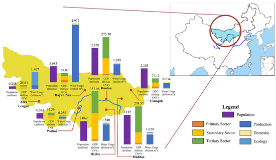
Figure 1.
Basic information of the seven prefectures connected by the Yellow River in Inner Mongolia. The population, GDP, and water usage of each sector in 2017 is shown.
This region in inland China has a semi-arid and arid climate zone, thus facing severe water shortages caused by low rainfall (Figure 2). The water resources per capita are 856 , which is approximately 1/7 of the world average [39]. In recent years, the rapidly growing economy has led to excessive water demand; however, declining groundwater levels, unstable precipitation, increasing temperatures, and frequent droughts have reduced the region’s water supply [36]. Industrial and urban water pollution contaminates water bodies and exacerbates the discordance between water supply and demand. This increasing disparity has restricted the region’s social and economic development [40]. In response to this growing concern, China has elevated ecological protection and high-quality development of the Yellow River Basin as a major national strategy, stressing the need for better water management in the region [41].
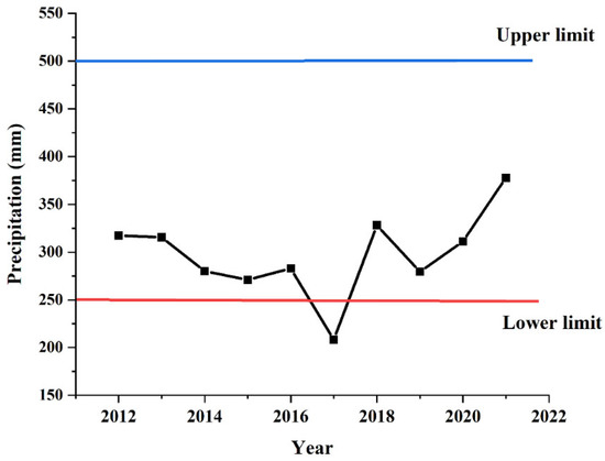
Figure 2.
Annual precipitation in Inner Mongolia from 2012 to 2021. Semi-arid climate is defined as having an annual precipitation of 250–500 mm; the lower and upper limits are depicted in the figure [42,43,44].
2.2. Hydro-Economic Model
The proposed hydro-economic model analyzes the effects of water availability on the economy. The relationship between water resources and economic output was assessed under different scenarios, including water conservation and climate change. The model integrates four sections using multiple constraints: (1) ecological, (2) economic, (3) social, and (4) environmental (Figure 3). The inputted data included information on regional water resources, economy, food production, and water pollution of the seven prefectures. Individual data collection was conducted for each prefecture to accommodate the divergent economic structures, as delineated in Figure 1, presenting substantial disparities in GDP and water consumption across distinct prefectures. Local data from 2017 and 2020 were collected to estimate future development on a 5-year basis until 2035 (2017, 2020, 2025, 2030, and 2035). We selected 2017 as the initial year because the most recent macroeconomic input–output table of Inner Mongolia was published in 2017. In addition, the data from 2017 were consistent with those from 2020, as the statistical calculation method for the regional data was adjusted in 2016.
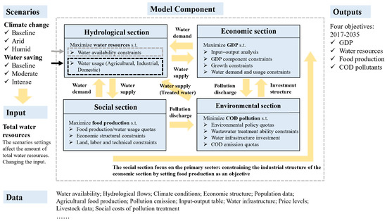
Figure 3.
Schematic of the hydro-economic model with constraints.
2.2.1. Ecological Section
The ecological objective is defined as:
where t represents each year of the simulated period, and d is each district within the studied area. This equation is subject to:
where is the total water usage in district d during year t, which is equal to the sum of the domestic water consumption and the water used for production in economic sector s. Equation (3) restrains water usage in each economic sector using the GDP of each sector, , and its water consumption quota, [28], and correlates the ecological and economic sections. The objective is defined as the amount of water resources, which is the sum of the amounts of surface water , groundwater , and treated water after subtracting total water usage [1].
Water availability and usage data were obtained from the Annual Inner Mongolia Water Resources Bulletin [45]. Water consumption quotas were obtained from the 2020 Inner Mongolia Sector Water Use Quota, published by the Inner Mongolia Water Resources Department [46]. The model was calibrated using the Inner Mongolia Statistical Yearbook and China Urban Construction Statistical Yearbook [47,48].
2.2.2. Economic Section
The economic objective can be written as follows:
which is subject to:
where is calculated based on input–output analysis [49,50], is the identity matrix, A is the reconciled direct consumption coefficient matrix, and is the economic output in sector s. The direct consumption coefficient matrix A is derived from the 42-sector input–output table for Inner Mongolia. However, the accessible input–output table treats Inner Mongolia as a whole, while the economic structures of different leagues vary considerably, resulting in different direct consumption coefficients. To ensure better prediction precision, we revised the bi-proportional scaling process (RAS method) and applied it to a direct consumption coefficient matrix. GDP is defined by summing its components: , the household consumption amount; , the household consumption distribution coefficient in economic sector s; , the social consumption amount; , the social consumption coefficient; , the fixed-asset investment amount; , the fixed-asset investment coefficient; , the current capital investment amount; , the current capital investment coefficient; , the amount of exports in sector s; and , the amount of imports. Equation (8) constrains the economic growth rate by imposing upper and lower growth limits, , respectively, to economic output.
The GDP data were collected from the Inner Mongolia Statistical Yearbook to calibrate the economic section. Economic data were obtained through calculations from the 42-sector input–output table of Inner Mongolia. The parameters and growth rates were set according to document requirements published by the state government of Inner Mongolia [51].
The RAS method was designed by Stone and Brown [52] and extensively tested by Bacharach [53]. The method updates a previously given input–output matrix within the predicted time period by reconciliating the columns and rows of the current matrix. Adjustments are made based on multipliers derived from limited data regarding the predicted period [54,55,56]. Using the RAS method in a broader context, Hewings [57] applied it to regionalize a known national input–output table. Mínguez [58] adopted a cell-corrected RAS method to use multiple input–output tables. In this study, instead of reconciliating the input–output table by year to fit future scenarios, as originally intended, we applied it to different districts, because the change in the direct consumption coefficient of each district within 20 years is relatively insignificant, as the economic structure is resistant to change owing to the endowment of resources and national food security requirements. Nevertheless, the pronounced spatial disparity in direct consumption coefficients across districts is discernible and can be attributed to differing economic structures, as evident in Figure 1.
Following the revised RAS method, was set as the initial direct consumption coefficient matrix; thus, the data can be collected from the 42-sector input–output table of Inner Mongolia (2017), with , as the total output of sector i in the predicted district league; , as the total intermediate output of sector in the predicted district league, and as the total intermediate input of sector in the predicted district league. The data for were derived from the 2017 Inner Mongolia Statistical Yearbook of 2017 [59]. The direct consumption coefficient matrix was reconciled as follows:
where can be derived from:
where Equations (12) and (15) define and after applying the RAS method for one iteration process, and . The iteration process, as shown in Equation (13), is repeated five times to ensure the RAS revision is thorough and complete.
2.2.3. Social Section
The social sector uses food production as an indicator of social welfare. The Yellow River in Inner Mongolia provides irrigation for one of China’s largest grain-producing areas, the Hetao Irrigation District [7]. Therefore, food production levels are correlated with national food security [60]. However, agriculture is a water-intensive industry with a relatively low economic output. In 2014, agriculture accounted for 63% of China’s water withdrawals but only 9% of the national GDP [60]. By neglecting the social objective, the model optimizes economic output by distributing all available water to the secondary and tertiary sectors, thereby jeopardizing food security. To highlight the importance of food safety and ensure that the amount of grain produced meets minimum food security standards, the social objective was set as the food production.
The social objective can be defined as:
which is subject to:
Equation (17) is the constraint set on food production, where the grain produced in tons in district d during year t is , food production per capita in the previous year is , lower growth limit of food production per capita is , and the total population is . Equation (18) links the social section with the economic section, where is the economic output in the primary sector, which is constrained by the lower () and upper () price limits of the primary sector, and total food production.
Agricultural data, namely grain production, population planting area, and economic output, were obtained from the Inner Mongolia Statistical Yearbook [59]. Agricultural prices were obtained from local agricultural trading websites [61,62]. The data were calibrated using legal documents published by the State Council [63,64].
2.2.4. Environmental Section
The environmental section analyzes the amount of chemical oxygen demand (COD) pollution to assess the environmental damage caused by water usage in the Yellow River. COD is the most common water pollution index in China [65]. Given global trends towards greater environmental awareness, the inclusion of environmental pollution in hydro-economic modeling has allowed models to become more coherent and consistent in achieving sustainable development [35,66].
The environmental objective can be expressed as:
which is subject to:
where the amount of COD pollutants is defined as the sum of pollutants in treated and untreated wastewater, is the treated water amount in district d during year t, is the total wastewater amount, is the level of pollutants per cubic meter of treated water, and is the level of pollutants per cubic meter of untreated water. Equation (21) focuses on treated water, which relies on the regional wastewater treatment rate, . Treated water is a variable that correlates the ecological and environmental sections. Equation (22) defines water investment costs as the sum of water treatment, water-saving, and building costs for sewage treatment plants, where is the treatment price per cubic meter of treated water, is the water-saving price per cubic meter of saved water, is the total amount of water consumption, is the price of building a sewage treatment plant, and is the number of sewage treatment plants. correlates the environmental sector with the economic sector, as it is added to the fixed-asset investment . The amount of treated water is constrained by the average sewage treatment capacity of the sewage treatment plants and the number of treatment plants .
Water pollution data were extracted from the Inner Mongolia Statistical Yearbook, Inner Mongolia Water Resources Bulletin, and China Urban Construction Statistical Yearbook [45,48,59,67]. The Inner Mongolia Statistical Yearbook provides data on the amount of COD pollutants emitted by each sector. Water usage in each sector and the amount of treated water were obtained from the Inner Mongolia Water Resources Bulletin. Data on sewage treatment plants and sewage treatment capacity were obtained from the China Urban Construction Statistical Yearbook. The COD abatement cost in Inner Mongolia was estimated as 8290 CNY/ton [68]. The water pollution parameters were obtained from the 2002 Discharge Standard of Pollutants for Municipal Wastewater Treatment Plant [67].
2.2.5. Optimization and Model Application
The optimization model integrates the four sections described above, and the optimization problem is given by:
The final objective is defined after normalizing the four objectives and assigning weights () to each. To determine their respective maximum and minimum values, the four objectives were simultaneously set as the final objectives for running the model. The maximum and minimum values of the four datasets for each objective were recorded during the normalization process. The weight of each objective was set according to policy inclination after discussion with local policy makers. The larger the weight, the more it is prioritized when outputting the results. In our study, the focus was primarily on economic and ecological objectives; therefore, the weight of these two objectives would be larger, making them more sensitive to changes in modeling conditions.
Determining the weights for optimization is a complex process. The weights should reflect the social context of the area, as well as the subjective preferences of stakeholders. The focus of this research is to discuss the hydro-economic relationship under different scenarios; however, we provide a more detailed discussion on the effect of weights on the objectives in Section 3.4. Future work could explore ways to accurately translate social context and stakeholders’ preferences into numerical weights. Furthermore, novel approaches such as distance-based multicriteria (e.g., compromise programming or the TOPSIS method) can be used to construct the objective function.
The mathematical programming package GAMS was used to compute the results. The model was solved using a linear programming algorithm under the Box–Jenkins model, a stochastic model used to simulate hydrological processes, to forecast the data ranges based on inputs from a given time series [69,70,71]. A linear approach was selected to incorporate the input–output table in the economic analysis [32]. Ward [72] indicated that GAMS is a useful tool for linear optimization because it is flexible, open, and self-documenting, thereby displaying the connections between the model formulation and solution.
2.3. Scenario Setup
The hydro-economic model was also used to assess the interdependence between water resources and economic productivity. Water availability is influenced by governmental water-saving policies and climatic conditions. The assessment of water-saving policies highlights the active intervention of public authorities and demonstrates their adaptability and effectiveness [1]. Climate change risk is critical in assessing water scarcity; thus, both high- and low-emission scenarios in the water literature were considered to gain an appropriate understanding of regional water availability [34].
The boundary conditions for water-saving intensity and climate change are given in Table 1 and Table 2, respectively. The data presented in Table 1 originate from the Water Consumption Quota of Inner Mongolia and the annual China Urban Construction Yearbook, both pivotal sources for water resource assessment [46,48]. The Water Consumption Quota delineates the specific water utilization levels pertinent to distinct industries, undergoing periodic revisions every five years within Inner Mongolia. Scrutiny of these quotas across varying years enabled us to discern and infer evolving policy trajectories concerning water conservation. Complementing this analysis, the China Urban Construction Yearbook furnishes a comprehensive district-wise breakdown of water consumption and wastewater management data for all provinces, offering a valuable adjunct for fine-tuning the trajectory depicted in water consumption quotas. Additionally, we calibrated our dataset employing the Inner Mongolia Water Resources Bulletin [39,45], a repository containing detailed accounts of water usage within diverse industries, documented annually. For prospective years, we relied upon the government development plans, articulated by the provincial administration of Inner Mongolia [64], which encapsulate forthcoming strategies aimed at water conservation. As for Table 2, the percentages are set based on past precipitation patterns and climate change predictions [73,74,75]. To refine and validate our parameters, we aligned our approach with data gleaned from the Inner Mongolia Water Resources Bulletin. The scenarios used in this study (Table 3) combine the boundary conditions of the two factors.

Table 1.
Boundary conditions for water-saving intensity for the study period.
Table 2.
Boundary conditions for climate change for the study period.
Table 3.
Various scenarios and their descriptions.
A coding method was used to name the scenarios. The two sets of digits represent the boundary conditions for water-saving intensity and climate change, as shown in Table 3. For example, scenario W0C2 implies present water-saving levels under an arid climate.
3. Results and Discussion
All nine possible scenarios were calculated using the proposed model. The weights of the four objectives were set to 5:1:1:5, based on discussion and agreement with local decision makers to approximate regional policy inclinations. See the Appendix A for a detailed discussion of all results.
3.1. Historical Data Validation
The results were validated using observational data from 2017 to 2021. From an eco-nomic perspective (Figure 4a), our simulated GDP was higher than the actual value because of price variation. The GDP before the COVID-19 pandemic and amount of water resources for all labeled years (Figure 4b) were projected with relative accuracy. The COVID-19 pandemic in 2020 likely caused production to all but cease, reducing GDP production and increasing water availability. In 2021, industries began to reopen on a larger scale, leading to an increasing pattern in the GDP and water resources. Along with COVID-19, previous literature discussed two other reasons that caused the decline in the GDP growth rate: (1) the downward growth rate of investments from 2015–2020 and (2) government policy restrictions on overheated industries [40,76,77]. In addition to unexpected incidents, the correlation between the model and reality indicated the existence of an empirical relationship, which allows future simulations to analyze the relationship between water resources and economic output.
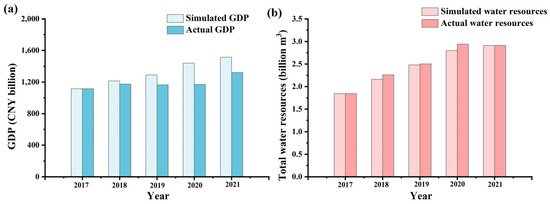
Figure 4.
Validation of simulated results for (a) GDP and (b) water resources using actual observation. Simulated results were obtained under present water-saving intensity and present climate conditions (scenario W0C0). Actual values were derived from the National Bureau of Statistics and the Department of Water Resources in Inner Mongolia.
3.2. Scenario Analysis
Table 4 shows the amounts of GDP, ecological water resources, food production, and COD pollutants for all scenarios in 2035. The results of the social objective (food production) and environmental objective (COD pollutants) validate the assumptions proposed in Section 2. Even when water is extremely scarce (scenario W0C2), food production maintains a red line of 9.57 million tons to ensure national food security. Moreover, food production levels minimally change from 9.99 million tons to 11.22 million tons when water becomes abundant (scenarios W0C1, W1C1, and W2C1), because the model prioritizes economic growth and water availability. Food production and water abundance in Inner Mongolia face a trade-off relationship, and increasing food production decreases water availability in the region [78]. This trade-off relationship is in line with our results, as water availability is prioritized over food production. Additionally, when facing structural economic changes, nonagricultural industries are expected to increase their share of water consumption at the expense of decreasing water use in agriculture. Water redistribution can lead to higher economic productivity. However, to ensure that food production remains at the red line, local farms must improve their irrigation efficiency to relax the trade-off relationship [29]. As a result, food security, water availability, and economic productivity must be ensured simultaneously.
Table 4.
Results of the nine scenarios based on the four indictors for 2035.
COD pollutant levels increase when the climate becomes more humid and decrease when more intense water-saving strategies are employed; however, the range of change is relatively limited. This finding highlights the differences between the two factors. When changes in water availability are induced by climate change, environmental pollution increases because more water is consumed. However, arid climates do not improve environmental quality because pollution concentrations increase as dilution processes worsen owing to water scarcity [1]. In contrast, if the changes are caused by water conservation, the pollution level declines because less water is consumed. COD pollution reduction levels are positively correlated with water-saving efficiency [68], indicating that water-saving policies can alleviate environmental pollution.
3.3. Effect of Water-Saving Strategies
To evaluate the effects of water resources on economic growth, Figure 5 shows the GDP output and average GDP growth rates under the different water scenarios. Figure 5a–c show the effect of water saving under a fixed climate scenario. Adopting water-saving strategies has a positive effect on economic growth, becoming more observable with a more arid climate. In Figure 5a, under present climate conditions, the 2035 GDP of scenarios W1C0 and W2C0 are 3058 and 3120 CNY billion, respectively, higher than that of scenario W0C0 (2579 CNY billion). The scenarios with and without water saving display a maximum discrepancy of 2% GDP growth rate. Under a humid climate, as demonstrated in Figure 5b, the benefits of water saving are reduced. The average annual GDP growth rates of the three scenarios remain roughly the same until 2035, with a difference of <0.05%. In 2035, when water becomes scarcer, the GDP growth rates of scenario W0C1, W1C1, and W2C1 drop to 2.5%, 3.3% and 3.0%, respectively. Figure 5c shows that the disparity between different water-saving scenarios is enlarged when the climate becomes increasingly arid. Without any water-saving measures (scenario W0C2), the annual GDP growth rate is halved to 5% in 2020 and decreases significantly to <1% in 2035, whereas Scenarios W0C0 and W0C1 are less influenced. This finding shows that water saving can counteract the negative effects of climate change.
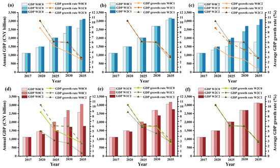
Figure 5.
Effect of different water scenarios on GDP. (a) Present climate, (b) humid climate, (c) arid climate, (d) present water-saving conditions, (b) moderate water-saving conditions, and (c) intense water-saving conditions. Annual GDP is the GDP of each labeled year on the x-axis. Average GDP growth rate is the annual GDP growth rate of 3/5 consecutive years calculated through exponential growth. For (a–c), all three water-saving intensities are presented under a fixed climate scenario. For (d–f), all three climate scenarios are depicted under a fixed water-saving intensity.
Figure 5d–f show the effects of climate change under a fixed water-saving intensity. An increasingly humid climate results in a rise in regional GDP. Figure 5d shows that under current water-saving intensities, the 2035 GDP of scenario W0C1 increases by 18% and 72% compared with those in scenarios W0C0 and W0C2, respectively. However, this increase was reduced to 4% and 15%, respectively, when a moderate water-saving approach was adopted (Figure 5e). This indicates that a moderate approach can be considered sufficient to sustain GDP development under present climate conditions, but it is still inadequate in arid conditions. As shown in Figure 5f, when water-saving conditions are intensified, the discrepancy is further reduced (to 0.4% and 1%). The GDP growth rates in the three scenarios display a maximum difference of 0.2%, confirming that intense water-saving policies can counteract the negative effects of arid climate.
Both water-saving strategies and humid climate change have a positive effect on macroeconomic performance. Humid climate change is positively correlated with economic productivity as it increases water availability. However, water saving is a complex problem. Although saving water reduces water availability and generates economic costs, our results show that these reductions do not necessarily negatively affect economic profitability. We expect that the cost of water saving will improve water-use efficiency, compensating for the negative effects of a reduced water supply. The economic profit from improved water has been proven to be greater than the cost of water saving. Previous studies have discovered that reductions in water usage in the primary, secondary, and tertiary sectors may lead to increased sector output if water-use efficiency is improved [29,30]. This finding is similar to our result at the macroeconomic scale. Thus, we inferred that the interactions between water resources and economic productivity depend on specific factors that affect water availability. An abundance of water resources lacking institutional strategies does not necessarily result in improved economic performance, even in arid regions.
A network-based approach was selected in this study, and through optimization and simulation, the interactions between multiple influencing factors were observed. Our results indicate that water-saving strategies are effective in counteracting the negative economic effects of climate change. The discrepancy between scenarios is least distinct when climate conditions are humid or when an intense water-saving strategy has been employed (Figure 5b,f). Previous studies have corroborated our findings by proving that under climate change and extreme weather conditions, water conservation practices can help mitigate damage and offer additional economic returns [79]. Additionally, the economic productivity of the worst climate scenario water-saving strategies could be better than that of the best climate scenario without water-saving strategies [80]. This is consistent with the results of this study, as the 2035 GDP of scenarios W0C1 and W2C2 (Table 4) show similar patterns. The combination of scenarios reflects the interactions between the influencing factors, because multiple factors can occur simultaneously. This method thus provides a more realistic approach for analyzing the interactions between water availability and economic productivity.
3.4. Trade-Off Relationship
Conserving water resources for ecological use incurs economic costs. To analyze the trade-off relationship between water resources protection and economic growth, we changed the weight of the economic and ecological objectives (from 1:9 to 7:1) to map a Pareto frontier. The weights of the social and environmental objectives remained unchanged at 1:1. Water-saving intensity and climate change are discussed in Figure 6 and Figure 7, respectively. Both figures show the other factors at the present levels (W0 and C0).
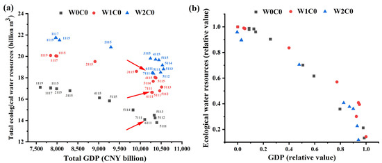
Figure 6.
Pareto frontier under different water-saving intensities. Total GDP and total water resources were calculated by summing the GDP and water resources of 2017, 2020, 2025, 2030, and 2035. (a) Absolute value; the weight of the four objectives is labeled at each point; for example. “1119” implies that the ratio of the weights of the economic, social, environmental and ecological objectives are 1:1:1:9. The red arrows indicate the area where the corresponding ratio between the economic and ecological objectives causes the Pareto frontier to reverse in direction. (b) Relative value, calculated through normalization to render the slope of the frontier more discernable.
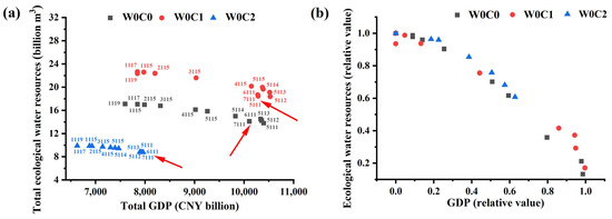
Figure 7.
Pareto frontier under different climate scenarios. (a) Absolute value and (b) relative value.
As shown in Figure 6a, under the same GDP, intensified water-saving rates can lead to more abundant water resources for ecological purposes, which is a Pareto improvement compared with the present conditions. In Figure 6b, the Pareto frontiers exhibit a near convergence, suggesting a robust and consistent interplay between water resource allocation and economic expansion. When the total GDP reaches 10,250 CNY billion, the trade-off relationship is more apparent for all three scenarios, as the slope of the frontier steepens. Increasing the ratio of economic and ecological objectives within each scenario increased GDP and decreased water resources. However, when the ratio reached 5:1 or 6:1 (red arrows in Figure 6a), the GDP output decreased with the amount of ecological water resources.
Climate change demonstrated patterns similar to those of the water-saving intensity, (Figure 7a). Under the same GDP, a more humid climate is considered a Pareto improvement. The frontier of scenario W0C2 shifted down and to the left, indicating that an arid climate with no water-saving strategies was Pareto-worsened in both economic and ecological terms. The Pareto frontiers in Figure 7a are almost parallel to each other, as indicated by the consistent relative value of the Pareto frontiers in Figure 7b. Compared with the Pareto frontiers in Figure 6, the GDP in Figure 7 is inversely related to ecological water resources until the ratio of the objectives reaches its turning point of 6:1 (red arrows in Figure 7a).
Water-saving policies and humid climate change lead to Pareto-improved shifts in the trade-off frontier, which is consistent with the results in Figure 5. Our results show that a trade-off exists between water resources protection and economic development, which is consistent with previous research [81,82]. This trade-off is more discernible when the total GDP output reaches a certain level, in this case, 10,250 CNY billion. Similar results were observed in the agricultural sector when irrigation was considered on a microeconomic scale. When total economic returns are <USD 300 million, reducing the value of all ecosystem services by 47% will increase economic returns by 83%. However, when economic returns are >USD 300 million, they increase by 51% at the expense of a 386% decline in ecosystem services [83]. A perceivable slope exists because before the turning point of 10,250 CNY billion, regional ecological water resources could still sustain development by regenerating themselves. However, water shortages begin to significantly constrain GDP as they continue to accumulate. These results highlight the trade-off between water protection and economic growth, emphasizing the need for effective water management.
Moreover, when the ratio between economic development and ecological water protection increases to 6:1, further focus on economic growth decreases economic output. This can be attributed to policies that lean excessively towards economic development; hence, water saving is omitted because it is costly and unprofitable. Rapid economic expansion is anticipated to precipitate an escalation in pollutant levels, necessitating more investments in water treatment. Given the non-linear cost dynamics associated with pollutant abatement, the consequent surge in investment for treatment is expected to reduce the total economic output. Although this approach can generate more economic profits in the short run, the deleterious effects of water shortages accumulate and eventually restrict economic growth. This indicates that when economic development is prioritized over ecological protection, output may suffer, as a lack of sufficient water resources limits economic growth.
3.5. Sensitivity Analysis and Robustness Testing
To extend the applicability of our hydro-economic model to diverse contexts and various regions, we conducted two validation tests to ascertain the robustness of our findings. Our first objective involved scrutinizing the sensitivity of pivotal parameters to mitigate the likelihood of biases in parameter selection. Subsequently, we validated our inferences using an expanded dataset encompassing a broader spectrum of scenarios, thereby reinforcing the credibility of our conclusions. Potential biases in parameter selection can potentially introduce inaccuracies. As our study mainly focuses on identifying the interactions between water resources and economic productivity, we selected four crucial parameters in Section 2.2.1 and Section 2.2.2 to test their sensitivity: the GDP lower and upper growth limits, and , respectively (Equation (8)), and the water consumption quotas for the secondary and tertiary sectors, and , respectively (Equation (3)). These parameters were adjusted to induce a specific percentage deviation from their initial values, ensuring that this deviation remains within a permissible range that does not compromise other critical constraints. All simulations were run under scenario W0C0 (baseline). The findings concerning the sensitivity of these essential parameters are presented in Figure 8.
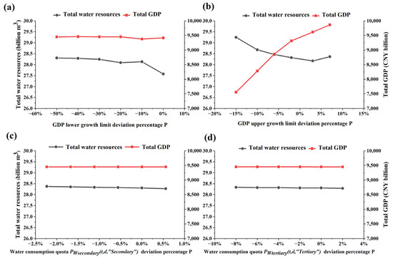
Figure 8.
Total GDP and total water resources when adjusting different paraments: (a) GDP lower growth limit , (b) GDP upper growth limit , (c) water consumption quota for the secondary sector , and (d) water consumption quota for the tertiary sector . The original parameter used in our model is the value when the deviation percentage is 0%.
As depicted in Figure 8, the overall volume of water resources exhibits notable insensitivity to adjustments in any of the parameters. Further focusing on the parameter eliciting the most significant fluctuation in total water resources (Figure 8b), the marginal discrepancy between the highest and lowest values is a mere 3.1%. This observation strongly suggests that outcomes concerning water resources remain largely resilient to potential biases stemming from parameter selection.
Conversely, the total GDP is impervious to alterations in merely three parameters, as delineated in Figure 8a,c,d. Specifically, Figure 8b highlights an absolute difference of 2309.79 billion CNY between the most stringent scenario (a −15% deviation, corresponding to a 0% per annum GDP upper growth limit) and the most lenient scenario for . To ensure the robustness of our results, especially concerning this sensitive parameter, we meticulously calibrated the upper growth limit by aligning it with historical data and anticipated government strategies. In the broader application of our model across various contexts, careful adjustments of this parameter are imperative to align with the unique economic landscapes of the respective regions.
Another pivotal consideration involves assessing the consistency and reliability of our findings across a more extensive dataset, encompassing a broader array of scenarios. Instead of confining our examination to the present, humid and arid climate conditions detailed in Table 2, we opted for a comprehensive approach. By utilizing the flow duration curve (FDC), we integrated climate conditions spanning documented historic years into our analysis. The FDC, illustrating the streamflow’s variability, establishes a relationship between streamflow rate and its exceedance percentage. For instance, a value of p = 25% signifies that 25% of historic years witnessed higher streamflow than the specified year. To approximate climate conditions accurately, we collected annual flow data, enabling a robust representation of hydrologic conditions and their impact on economic productivity. This methodological approach enhances our ability to elucidate the influence of varied hydrological contexts on the economic output, as illustrated in Figure 9.
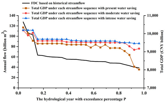
Figure 9.
Relationship between total GDP and the FDC under different water-saving conditions. The horizontal axis represents the specific hydrologic years arrayed by the exceedance percentage, and each hydrologic year corresponds to a specific total GDP output.
Figure 9 demonstrates similar patterns to those observed in our earlier results presented in Figure 5. Notably, when the exceedance percentage P falls below 50%, signifying ample water resources and a relatively humid climate based on historical records, the distinctions among the three water-saving scenarios are minimal. This suggests that implementing water-saving measures yields limited benefits in humid climates. However, as the exceedance percentage P surpasses 50%, a decline in GDP output becomes evident for the current water-saving scenario. The variations between moderate and intense water-saving strategies remain relatively subtle and consistent. As the exceedance percentage P reaches 85%, the gap between the three water-saving strategies widens, underscoring the emerging advantages of an intense water-saving approach. While our research places importance on data accuracy and precision, our findings exhibit a degree of robustness when considering diverse datasets.
In spite of conducting a sensitivity analysis on our parameters and verifying the robustness of our findings, potential limitations must be acknowledged before drawing definitive conclusions when extending the model to diverse regions. Our study necessitated certain assumptions regarding the model’s parameters to capture and describe the context of our study region. For example, we assumed an upper limit of 12% for the annual GDP growth rate, a premise below the growth rates observed in several countries like Armenia and Monaco [84]. Similarly, we enforced strict boundary conditions to prioritize the production levels within the primary sector to align with national food security goals, particularly pertinent to China but potentially differing in other regions. Another postulation of this study is the enduring stability of input–output tables over time, attributed to the persisting regional economic framework. Consequently, we have implemented the RAS method across various districts. When transitioning this model to alternative regions, these parameters must be flexibly adjusted to mirror their unique contextual dynamics. The parameters, while specific, underlie a general model structure. To ensure precise and reliable conclusions in different regions, recalibration of these parameters in accordance with updated assumptions is indispensable.
3.6. Policy Implications
This study assessed water-saving strategies to enhance economic productivity and mitigate climate change impacts, demonstrating the synergy between climate change and water resources management [85]. Our methodology aligns with the 17 Sustainable Development Goals (SDG) outlined by the United Nations, particularly SDG 6, which advocates for sustainable water management [86], and SDG 13, which urges action against climate change [87]. Our results call for an integrated approach engaging various stakeholders while recognizing the interconnectedness of water resources across diverse sectors within society [88].
Economic productivity does not necessarily increase with intensified water-saving policies. Amidst humid climate conditions, when water resources increase by 6% every 5 years, the benefits of water saving remain limited. A moderate water-saving approach appears sufficient to sustain GDP development within the prevailing climate parameters. However, when water resources decrease by 6% every 5 years, an intensified water-saving strategy becomes imperative to mitigate the adverse effects of climatic uncertainty. Stakeholders must adjust water-saving rates accordingly with different climate settings. Possible measures proven to be beneficial to economic growth include agricultural and industrial technology improvement, industrial water reuse, and structural adjustment towards the tertiary sector [30]. However, the realistic adoption of specific policies hinges on critical factors, such as cost-effectiveness and associated transaction costs. Effectively implementing policies necessitates their alignment with social acceptability, along with the integration of enforcement mechanisms to ensure stakeholder compliance [1].
The choice of policies depends on the objectives of decision-makers. We focused on the interactions between the ecological, economic, social, and environmental components of the region. Based on our findings, COD pollutant levels increase with humidity but decrease with intensive water-saving methods. This outcome underscores the environmental and economic trade-offs associated with policy decisions. Although water-saving strategies have limitations in humid climates [89], they demonstrate the potential to mitigate pollution levels. From a societal perspective, food production levels must remain relatively stable to uphold social stability. Therefore, any structural adjustments in policies for the region should carefully consider food security. Implementing more water-efficient policies within the agricultural sector emerges as a promising avenue to effectively navigate these multifaceted considerations. In terms of the economic and the ecological objectives, we identified the critical threshold ratio of 6:1, in which an excessive focus on economic productivity will harm both goals. This trade-off underscores a vital consideration for policymakers, providing a quantifiable measure that ensures sustainability within the framework of development.
However, some limitations remain. The proposed hydro-economic model was linear, to incorporate input–output analysis in the economic section and understand the sectoral relationships of water from a macroeconomic perspective. This approach may affect the simulation results by simplifying nonlinear conditions, such as flexible variability in substitution across inputs and diminishing marginal returns of increased input use [32]. Moreover, although the model has been calibrated, data availability and precision remain a challenge when simulating future conditions over a multi-year horizon. Because simulation models are heavily data-dependent, regions lacking comprehensive and high-quality databases, particularly within emerging economies, face challenges in model reproduction. Despite these shortcomings, our hydro-economic model provides an analytical tool for simulating interactions between water resources and economic productivity.
Future research should conduct a more comprehensive investigation into specific water-saving strategies (i.e., technological advancements, structural adjustments, and water reuse) and assess their efficiencies under different scenarios. Specifically, an examination of the comparative advantages of these distinct approaches across various sectors, regions, and temporal domains can assist policymakers in formulating enhanced and informed decisions. Another potential improvement is to incorporate nonlinear constraints in production processes. This could enhance the precision of the simulation model, given the persistence of input–output analysis.
4. Conclusions
This study modeled hydrological–economic interactions for sustainable development in an arid to semi-arid region. Our study is novel in three key aspects: First, the developed network-based hydro-economic model using simulation and optimization effectively assessed the combination of different scenarios in an integrated manner. Second, the bi-proportional scaling process (RAS) method was adapted to accommodate variations in spatial attributes across districts. Third, climate change impacts were considered, and the efficiency of policy intervention was analyzed under the context of climate adaptability.
Our assessment considered both economic productivity and climate adaptability, revealing the complicated interactions between water resources and sustainable development and the role of water-saving policies on enhancing regional economic development by improving water use efficiency. Under several modelling assumptions, water-saving initiatives limited the impact on economic growth enhancement under humid climate conditions. We determined that a balanced approach is adequate to sustain GDP growth in the current climate. However, arid climates necessitate a more aggressive water-saving strategy to counteract climate uncertainties. Notably, the economic productivity in the harshest climate scenario (2035 GDP of 3101.56 CNY billion) could potentially surpass the outcomes in the most favorable climate scenario (2035 GDP of 3053.17 CNY billion) when applying water-saving strategies. Furthermore, the trade-off between water resources protection and economic development becomes more apparent when water resources are depleted. Water saving and humid climate change both result in Pareto-improved frontiers. In particular, when the weight ratio between the economic and ecological objectives reached its turning point of 6:1, further emphasis on economic development negatively affected both objectives.
These findings underscore the role of water conservation in fortifying climate adaptability and propelling societal resilience. The quantitative evaluation of hydrological–economic interactions can provide managerial insights and a decision-making basis for sustainability in water-deficient regions. When considering the entire macroeconomic system in a region, policy priorities must be carefully determined, as all objectives cannot be pursued simultaneously with the trade-off relationship. The modeling approach proposed in this study provides a theoretical basis for future analyses of the effects of water resources on sustainable development, especially in arid and semi-arid regions with similar climate conditions.
Author Contributions
Conceptualization, J.Z. (Jianshi Zhao) and H.Z.; methodology, H.Z. and S.C.; software, J.Z. (Jinghao Zhang); validation, S.C., J.Z. (Jinghao Zhang) and H.Z.; data curation, J.Z. (Jinghao Zhang), S.C. and H.Z.; writing—original draft preparation, H.Z.; writing—review and editing, J.Z. (Jianshi Zhao) and H.Z.; visualization, J.Z. (Jinghao Zhang) and H.Z.; supervision, S.C. and J.Z. (Jianshi Zhao); project administration, J.Z. (Jianshi Zhao); funding acquisition, J.Z. (Jianshi Zhao). All authors have read and agreed to the published version of the manuscript.
Funding
This research was supported by the National Key Research and Development Program of China (Grant No. 2021YFC3201204) and the National Natural Science Foundation of China (U2243215 and 42041004).
Institutional Review Board Statement
Not applicable.
Informed Consent Statement
Not applicable.
Data Availability Statement
Data are contained within the article.
Conflicts of Interest
The authors declare no conflicts of interest.
Appendix A
We provide the details to our results and coefficients in the tables below. The notation for all following tables is: GDP (Billion CNY), FOOD for Food production (Million tons), COD for COD pollutants (Thousand tons) and GREEN Ecological water resources (Billion m3).
Table A1.
Effect of Water-Saving Strategies (Section 3.3).
Table A1.
Effect of Water-Saving Strategies (Section 3.3).
| Scenario | Objective | 2017 | 2020 | 2025 | 2030 | 2035 |
|---|---|---|---|---|---|---|
| W0C0 | GDP | 1114.64 | 1438.54 | 1860.21 | 2266.2 | 2578.85 |
| FOOD | 9.57 | 9.57 | 9.57 | 9.57 | 9.57 | |
| COD | 398.94 | 360.3 | 337.62 | 322.29 | 313.16 | |
| GREEN | 1.84 | 2.8 | 3.37 | 3.79 | 4.04 | |
| W0C1 | GDP | 1114.64 | 1496.54 | 2014.06 | 2694.13 | 3053.17 |
| FOOD | 9.57 | 9.58 | 9.63 | 9.69 | 9.99 | |
| COD | 398.94 | 364.18 | 346.28 | 339.75 | 334.58 | |
| GREEN | 1.84 | 3.07 | 4.16 | 5 | 5.89 | |
| W0C2 | GDP | 1114.64 | 1291.15 | 1508.49 | 1714.3 | 1764.98 |
| FOOD | 9.57 | 9.57 | 9.57 | 9.57 | 9.57 | |
| COD | 398.94 | 357.63 | 331.47 | 314.44 | 302.75 | |
| GREEN | 1.84 | 1.9 | 2.03 | 1.97 | 1.78 | |
| W1C0 | GDP | 1114.64 | 1496.53 | 2014.97 | 2689.78 | 3057.77 |
| FOOD | 9.57 | 9.58 | 9.63 | 9.76 | 10.2 | |
| COD | 398.94 | 350.47 | 313.31 | 288.97 | 269.59 | |
| GREEN | 1.84 | 3.01 | 3.87 | 4.41 | 4.86 | |
| W1C1 | GDP | 1114.64 | 1496.56 | 2015.91 | 2702.5 | 3175.68 |
| FOOD | 9.57 | 9.67 | 10.08 | 10.6 | 11.22 | |
| COD | 398.94 | 352.05 | 319.21 | 299.38 | 283.17 | |
| GREEN | 1.84 | 3.35 | 4.76 | 5.89 | 6.98 | |
| W1C2 | GDP | 1114.64 | 1438.54 | 1909.14 | 2387.66 | 2752.35 |
| FOOD | 9.57 | 9.57 | 9.57 | 9.57 | 9.57 | |
| COD | 398.94 | 347.38 | 308.46 | 279.91 | 257.84 | |
| GREEN | 1.84 | 2.1 | 2.44 | 2.58 | 2.58 | |
| W2C0 | GDP | 1114.64 | 1496.57 | 2015.89 | 2698.76 | 3120.05 |
| FOOD | 9.57 | 9.67 | 9.84 | 10.1 | 10.68 | |
| COD | 398.94 | 351.43 | 298.42 | 258.84 | 233.97 | |
| GREEN | 1.84 | 2.99 | 4.18 | 5.04 | 5.6 | |
| W2C1 | GDP | 1114.64 | 1496.56 | 2015.88 | 2699.84 | 3133.9 |
| FOOD | 9.57 | 9.67 | 9.84 | 10.1 | 10.68 | |
| COD | 398.94 | 352.05 | 299.02 | 259.43 | 234.69 | |
| GREEN | 1.84 | 3.35 | 5.2 | 6.76 | 8.04 | |
| W2C2 | GDP | 1114.64 | 1494.21 | 2013.96 | 2699.71 | 3101.56 |
| FOOD | 9.57 | 9.57 | 9.57 | 9.57 | 9.65 | |
| COD | 398.94 | 349.39 | 294.07 | 252.85 | 223.54 | |
| GREEN | 1.84 | 2.05 | 2.73 | 3.09 | 3.25 |
Table A2.
Trade-off Relationships (Section 3.4).
Table A2.
Trade-off Relationships (Section 3.4).
| Case: W0C0 | ||||||
|---|---|---|---|---|---|---|
| Pareto Scenario | Objective | 2017 | 2020 | 2025 | 2030 | 2035 |
| 1115 | GDP | 1114.64 | 1340.83 | 1614.49 | 1802.19 | 1973.25 |
| GREEN | 1.84 | 2.9 | 3.63 | 4.15 | 4.52 | |
| 1117 | GDP | 1114.64 | 1340.83 | 1614.49 | 1802.19 | 1973.25 |
| GREEN | 1.84 | 2.91 | 3.64 | 4.16 | 4.52 | |
| 1119 | GDP | 1114.64 | 1313.87 | 1539.17 | 1728.53 | 1900.32 |
| GREEN | 1.84 | 2.91 | 3.65 | 4.17 | 4.53 | |
| 2115 | GDP | 1114.64 | 1341.15 | 1620.54 | 1844.95 | 2067.2 |
| GREEN | 1.84 | 2.91 | 3.63 | 4.13 | 4.46 | |
| 3115 | GDP | 1114.64 | 1343.86 | 1643.72 | 1979.05 | 2227.86 |
| GREEN | 1.84 | 2.9 | 3.6 | 4.06 | 4.38 | |
| 4115 | GDP | 1114.64 | 1438.53 | 1785.69 | 2185.36 | 2493.2 |
| GREEN | 1.84 | 2.8 | 3.45 | 3.89 | 4.15 | |
| 5115 | GDP | 1114.64 | 1438.54 | 1860.21 | 2266.2 | 2578.85 |
| GREEN | 1.84 | 2.8 | 3.37 | 3.79 | 4.04 | |
| 5114 | GDP | 1114.64 | 1483.83 | 1988.86 | 2457.52 | 2780.01 |
| GREEN | 1.84 | 2.73 | 3.19 | 3.53 | 3.69 | |
| 5113 | GDP | 1114.64 | 1495.82 | 2014.25 | 2668.85 | 3039.16 |
| GREEN | 1.84 | 2.71 | 3.15 | 3.31 | 3.49 | |
| 5112 | GDP | 1114.64 | 1496.28 | 2015.82 | 2663.83 | 3063.51 |
| GREEN | 1.84 | 2.68 | 3.08 | 3.24 | 3.4 | |
| 5111 | GDP | 1114.64 | 1499.77 | 2018.99 | 2668.92 | 3092.26 |
| GREEN | 1.84 | 2.65 | 3 | 3.11 | 3.21 | |
| 6111 | GDP | 1114.64 | 1498.07 | 2009.47 | 2592.98 | 2923.89 |
| GREEN | 1.84 | 2.63 | 3.06 | 3.25 | 3.42 | |
| 7111 | GDP | 1114.64 | 1502.34 | 2013.97 | 2582.89 | 2891.87 |
| GREEN | 1.84 | 2.6 | 3.02 | 3.22 | 3.42 | |
| Case: W1C0 | ||||||
| Pareto Scenario | Objective | 2017 | 2020 | 2025 | 2030 | 2035 |
| 1115 | GDP | 1114.64 | 1340.83 | 1619.8 | 1844.17 | 2073.12 |
| GREEN | 1.84 | 3.2 | 4.28 | 5.07 | 5.65 | |
| 1117 | GDP | 1114.64 | 1340.83 | 1614.99 | 1839.8 | 2061.31 |
| GREEN | 1.84 | 3.2 | 4.28 | 5.07 | 5.66 | |
| 1119 | GDP | 1114.64 | 1340.83 | 1613.56 | 1802.17 | 1973.23 |
| GREEN | 1.84 | 3.2 | 4.28 | 5.08 | 5.69 | |
| 2115 | GDP | 1114.64 | 1382.41 | 1785.54 | 2152.26 | 2476.07 |
| GREEN | 1.84 | 3.16 | 4.16 | 4.92 | 5.44 | |
| 3115 | GDP | 1114.64 | 1452.04 | 1939.12 | 2496.36 | 2905.08 |
| GREEN | 1.84 | 3.08 | 4 | 4.62 | 5.06 | |
| 4115 | GDP | 1114.64 | 1495.82 | 2013.34 | 2686.98 | 3041.8 |
| GREEN | 1.84 | 3.01 | 3.88 | 4.42 | 4.88 | |
| 5115 | GDP | 1114.64 | 1496.53 | 2014.97 | 2689.78 | 3057.77 |
| GREEN | 1.84 | 3.01 | 3.87 | 4.41 | 4.86 | |
| 5114 | GDP | 1114.64 | 1493.6 | 2005.57 | 2662.64 | 3033.4 |
| GREEN | 1.84 | 2.97 | 3.81 | 4.33 | 4.72 | |
| 5113 | GDP | 1114.64 | 1498.07 | 2017.76 | 2700.08 | 3181.53 |
| GREEN | 1.84 | 2.96 | 3.71 | 4.15 | 4.47 | |
| 5112 | GDP | 1114.64 | 1498.38 | 2017.41 | 2676.05 | 3158.09 |
| GREEN | 1.84 | 2.91 | 3.63 | 4.04 | 4.36 | |
| 5111 | GDP | 1114.64 | 1502.2 | 2017.14 | 2656.37 | 2985.33 |
| GREEN | 1.84 | 2.85 | 3.56 | 4.04 | 4.34 | |
| 6111 | GDP | 1114.64 | 1502.27 | 2015.59 | 2654.61 | 2984.41 |
| GREEN | 1.84 | 2.85 | 3.57 | 4.05 | 4.35 | |
| 7111 | GDP | 1114.64 | 1502.82 | 2016.08 | 2655.36 | 2998.12 |
| GREEN | 1.84 | 2.84 | 3.56 | 4.04 | 4.34 | |
| Case: W2C0 | ||||||
| Pareto Scenario | Objective | 2017 | 2020 | 2025 | 2030 | 2035 |
| 1115 | GDP | 1114.64 | 1340.84 | 1624.5 | 1868.38 | 2109.62 |
| GREEN | 1.84 | 3.19 | 4.58 | 5.63 | 6.27 | |
| 1117 | GDP | 1114.64 | 1340.83 | 1615.23 | 1840.55 | 2062.33 |
| GREEN | 1.84 | 3.2 | 4.62 | 5.69 | 6.39 | |
| 1119 | GDP | 1114.64 | 1340.83 | 1613.63 | 1837.86 | 2058.56 |
| GREEN | 1.84 | 3.2 | 4.62 | 5.7 | 6.39 | |
| 2115 | GDP | 1114.64 | 1435.18 | 1872.17 | 2266.55 | 2603.53 |
| GREEN | 1.84 | 3.12 | 4.41 | 5.43 | 6.05 | |
| 3115 | GDP | 1114.64 | 1480.65 | 1988.61 | 2649.81 | 3008.34 |
| GREEN | 1.84 | 3.01 | 4.22 | 5.08 | 5.66 | |
| 4115 | GDP | 1114.64 | 1495.82 | 2014.17 | 2691.59 | 3048.36 |
| GREEN | 1.84 | 2.99 | 4.19 | 5.05 | 5.64 | |
| 5115 | GDP | 1114.64 | 1496.57 | 2015.89 | 2698.76 | 3120.05 |
| GREEN | 1.84 | 2.99 | 4.18 | 5.04 | 5.6 | |
| 5114 | GDP | 1114.64 | 1496.61 | 2018.41 | 2703.73 | 3196.79 |
| GREEN | 1.84 | 2.97 | 4.09 | 4.89 | 5.39 | |
| 5113 | GDP | 1114.64 | 1499.44 | 2019.84 | 2700.28 | 3222.49 |
| GREEN | 1.84 | 2.89 | 4.01 | 4.79 | 5.27 | |
| 5112 | GDP | 1114.64 | 1498.23 | 2019.45 | 2678.81 | 3175.49 |
| GREEN | 1.84 | 2.85 | 3.93 | 4.7 | 5.19 | |
| 5111 | GDP | 1114.64 | 1502.31 | 2017.57 | 2657.03 | 2997.67 |
| GREEN | 1.84 | 2.84 | 3.93 | 4.68 | 5.17 | |
| 6111 | GDP | 1114.64 | 1502.31 | 2015.94 | 2655.47 | 3015.75 |
| GREEN | 1.84 | 2.84 | 3.93 | 4.68 | 5.15 | |
| 7111 | GDP | 1114.64 | 1502.76 | 2018.02 | 2658.14 | 3019.99 |
| GREEN | 1.84 | 2.84 | 3.92 | 4.67 | 5.13 | |
| Case: W0C1 | ||||||
| Pareto Scenario | Objective | 2017 | 2020 | 2025 | 2030 | 2035 |
| 1115 | GDP | 1114.64 | 1340.83 | 1628.62 | 1888.3 | 2148.17 |
| GREEN | 1.84 | 3.56 | 5.6 | 7.32 | 8.7 | |
| 1117 | GDP | 1114.64 | 1340.83 | 1619.05 | 1844.38 | 2071.46 |
| GREEN | 1.84 | 3.58 | 5.66 | 7.43 | 8.86 | |
| 1119 | GDP | 1114.64 | 1340.83 | 1615.04 | 1839.85 | 2061.36 |
| GREEN | 1.84 | 3.58 | 5.66 | 7.43 | 8.86 | |
| 2115 | GDP | 1114.64 | 1438.52 | 1876.14 | 2319.89 | 2701.1 |
| GREEN | 1.84 | 3.47 | 5.41 | 7.07 | 8.34 | |
| 3115 | GDP | 1114.64 | 1483.01 | 1994.8 | 2554.25 | 2883.91 |
| GREEN | 1.84 | 3.39 | 5.25 | 6.8 | 8.12 | |
| 4115 | GDP | 1114.64 | 1496.54 | 2014.94 | 2687.27 | 3051.38 |
| GREEN | 1.84 | 3.37 | 5.23 | 6.73 | 8.04 | |
| 5115 | GDP | 1114.64 | 1496.56 | 2018.51 | 2703.3 | 3191.5 |
| GREEN | 1.84 | 3.36 | 5.21 | 6.7 | 7.96 | |
| 5114 | GDP | 1114.64 | 1496.69 | 2018.93 | 2705 | 3238.38 |
| GREEN | 1.84 | 3.28 | 5.06 | 6.55 | 7.78 | |
| 5113 | GDP | 1114.64 | 1498.23 | 2017.19 | 2661.84 | 3157.54 |
| GREEN | 1.84 | 3.23 | 4.98 | 6.46 | 7.69 | |
| 5112 | GDP | 1114.64 | 1498.07 | 2012.67 | 2652.23 | 2994.44 |
| GREEN | 1.84 | 3.24 | 5.04 | 6.56 | 7.87 | |
| 5111 | GDP | 1114.64 | 1502.09 | 2017.58 | 2657.32 | 3004.84 |
| GREEN | 1.84 | 3.23 | 4.91 | 6.35 | 7.57 | |
| 6111 | GDP | 1114.64 | 1502.44 | 2016.36 | 2655.74 | 3008.24 |
| GREEN | 1.84 | 3.21 | 4.89 | 6.34 | 7.55 | |
| 7111 | GDP | 1114.64 | 1502.76 | 2018.31 | 2659.93 | 3031.17 |
| GREEN | 1.84 | 3.2 | 4.88 | 6.3 | 7.51 | |
| Case: W0C2 | ||||||
| Pareto Scenario | Objective | 2017 | 2020 | 2025 | 2030 | 2035 |
| 1115 | GDP | 1114.64 | 1279.28 | 1456.5 | 1516.77 | 1509.53 |
| GREEN | 1.84 | 1.92 | 2.09 | 2.07 | 1.93 | |
| 1117 | GDP | 1114.64 | 1252.32 | 1382.06 | 1443.07 | 1436.58 |
| GREEN | 1.84 | 1.93 | 2.1 | 2.08 | 1.94 | |
| 1119 | GDP | 1114.64 | 1252.32 | 1382.06 | 1443.07 | 1436.58 |
| GREEN | 1.84 | 1.93 | 2.1 | 2.08 | 1.94 | |
| 2115 | GDP | 1114.64 | 1279.28 | 1466.81 | 1538.16 | 1530.71 |
| GREEN | 1.84 | 1.92 | 2.09 | 2.06 | 1.93 | |
| 3115 | GDP | 1114.64 | 1280.1 | 1488.12 | 1622.52 | 1636.86 |
| GREEN | 1.84 | 1.92 | 2.07 | 2.02 | 1.87 | |
| 4115 | GDP | 1114.64 | 1286.87 | 1495 | 1674.95 | 1730.81 |
| GREEN | 1.84 | 1.91 | 2.05 | 2 | 1.81 | |
| 5115 | GDP | 1114.64 | 1291.15 | 1508.49 | 1714.3 | 1764.98 |
| GREEN | 1.84 | 1.9 | 2.03 | 1.97 | 1.78 | |
| 5114 | GDP | 1114.64 | 1291.18 | 1508.66 | 1745.8 | 1805.65 |
| GREEN | 1.84 | 1.89 | 2.01 | 1.94 | 1.75 | |
| 5113 | GDP | 1114.64 | 1334.96 | 1625.18 | 1880.63 | 1944.9 |
| GREEN | 1.84 | 1.83 | 1.85 | 1.75 | 1.56 | |
| 5112 | GDP | 1114.64 | 1334.96 | 1615.53 | 1883.16 | 1946.28 |
| GREEN | 1.84 | 1.83 | 1.85 | 1.75 | 1.56 | |
| 5111 | GDP | 1114.64 | 1339.66 | 1629.95 | 1905.37 | 1971.72 |
| GREEN | 1.84 | 1.82 | 1.84 | 1.73 | 1.54 | |
| 6111 | GDP | 1114.64 | 1338.44 | 1628.75 | 1898.58 | 1943.86 |
| GREEN | 1.84 | 1.82 | 1.83 | 1.72 | 1.54 | |
| 7111 | GDP | 1114.64 | 1342.54 | 1632.81 | 1903.26 | 1949.19 |
| GREEN | 1.84 | 1.81 | 1.83 | 1.73 | 1.54 |
Table A3.
GDP lower growth limit deviation (Section 3.5).
Table A3.
GDP lower growth limit deviation (Section 3.5).
| GDP Lower Growth Deviation (%) | Objective | 2017 | 2020 | 2025 | 2030 | 2035 |
|---|---|---|---|---|---|---|
| −50.0 | GDP | 1114.64 | 1494.27 | 1994.51 | 2342.07 | 2506.48 |
| FOOD | 9.57 | 6.77 | 4.85 | 3.49 | 2.53 | |
| COD | 398.94 | 266.49 | 207.35 | 176.11 | 154.95 | |
| GREEN | 1.84 | 5.01 | 6.42 | 7.22 | 7.82 | |
| −40.0 | GDP | 1114.64 | 1495.74 | 1991.24 | 2336.96 | 2521.77 |
| FOOD | 9.57 | 6.77 | 4.85 | 3.49 | 2.53 | |
| COD | 398.94 | 266.68 | 207.26 | 176.22 | 155.28 | |
| GREEN | 1.84 | 5 | 6.42 | 7.22 | 7.81 | |
| −30.0 | GDP | 1114.64 | 1494.94 | 1960.21 | 2347.76 | 2538.1 |
| FOOD | 9.57 | 6.77 | 4.85 | 3.49 | 2.68 | |
| COD | 398.94 | 266.85 | 206.49 | 176.45 | 157.58 | |
| GREEN | 1.84 | 5 | 6.44 | 7.21 | 7.75 | |
| −20.0 | GDP | 1114.64 | 1490.08 | 1968.86 | 2325.49 | 2555.79 |
| FOOD | 9.57 | 6.77 | 4.85 | 3.49 | 3.03 | |
| COD | 398.94 | 266.74 | 206.89 | 176.37 | 163.46 | |
| GREEN | 1.84 | 5.01 | 6.43 | 7.21 | 7.59 | |
| −10.0 | GDP | 1114.64 | 1469.7 | 1963.29 | 2300.85 | 2531.69 |
| FOOD | 9.57 | 6.77 | 4.85 | 3.49 | 2.88 | |
| COD | 398.94 | 266.42 | 207.06 | 175.99 | 162.14 | |
| GREEN | 1.84 | 5.02 | 6.43 | 7.23 | 7.61 | |
| 0 | GDP | 1114.64 | 1479.73 | 1985.14 | 2337.51 | 2500.87 |
| FOOD | 9.57 | 6.77 | 4.85 | 3.49 | 2.88 | |
| COD | 398.94 | 267.36 | 210.12 | 183.01 | 171.64 | |
| GREEN | 1.84 | 4.99 | 6.36 | 7.04 | 7.35 |
Table A4.
GDP upper growth limit deviation (Section 3.5).
Table A4.
GDP upper growth limit deviation (Section 3.5).
| GDP Upper Growth Deviation (%) | Objective | 2017 | 2020 | 2025 | 2030 | 2035 |
|---|---|---|---|---|---|---|
| −14.5 | GDP | 1114.64 | 1285.81 | 1487.24 | 1708.37 | 1960.43 |
| FOOD | 9.57 | 6.77 | 4.85 | 3.49 | 2.54 | |
| COD | 398.94 | 261.06 | 196.05 | 163.43 | 146.93 | |
| GREEN | 1.84 | 5.16 | 6.74 | 7.54 | 7.97 | |
| −10.3 | GDP | 1114.64 | 1342.23 | 1620.56 | 1951.76 | 2255.88 |
| FOOD | 9.57 | 6.77 | 4.85 | 3.49 | 2.53 | |
| COD | 398.94 | 263.39 | 199.9 | 171.22 | 155.1 | |
| GREEN | 1.84 | 5.1 | 6.63 | 7.33 | 7.77 | |
| −6.0 | GDP | 1114.64 | 1405.8 | 1770.94 | 2206.45 | 2368.99 |
| FOOD | 9.57 | 6.77 | 4.85 | 3.49 | 2.53 | |
| COD | 398.94 | 264.69 | 202.76 | 175.25 | 154.99 | |
| GREEN | 1.84 | 5.06 | 6.55 | 7.22 | 7.79 | |
| −1.7 | GDP | 1114.64 | 1467.57 | 1929.14 | 2319.84 | 2486.17 |
| FOOD | 9.57 | 6.77 | 4.85 | 3.49 | 2.53 | |
| COD | 398.94 | 266 | 206.22 | 176.4 | 155.52 | |
| GREEN | 1.84 | 5.02 | 6.45 | 7.21 | 7.79 | |
| 2.6 | GDP | 1114.64 | 1529.22 | 2091.76 | 2386.4 | 2549.45 |
| FOOD | 9.57 | 6.77 | 4.85 | 3.49 | 2.53 | |
| COD | 398.94 | 266.97 | 209.69 | 177.53 | 156.09 | |
| GREEN | 1.84 | 4.99 | 6.35 | 7.19 | 7.79 | |
| 6.8 | GDP | 1114.64 | 1590.4 | 2212.92 | 2412.73 | 2535.6 |
| FOOD | 9.57 | 6.79 | 4.86 | 3.5 | 2.6 | |
| COD | 398.94 | 268.23 | 209.59 | 173.89 | 151.52 | |
| GREEN | 1.84 | 4.96 | 6.34 | 7.29 | 7.93 |
Table A5.
Water consumption quota deviation for the secondary sector (Section 3.5).
Table A5.
Water consumption quota deviation for the secondary sector (Section 3.5).
| Water Consumption Quota Deviation (%) | Objective | 2017 | 2020 | 2025 | 2030 | 2035 |
|---|---|---|---|---|---|---|
| −2.23 | GDP | 1114.64 | 1494.27 | 1994.53 | 2342.08 | 2506.66 |
| FOOD | 9.57 | 6.79 | 4.86 | 3.5 | 2.53 | |
| COD | 398.59 | 266.22 | 206.88 | 175.6 | 154.49 | |
| GREEN | 1.86 | 5.02 | 6.43 | 7.24 | 7.83 | |
| −1.68 | GDP | 1114.64 | 1494.27 | 1994.53 | 2342.08 | 2506.66 |
| FOOD | 9.57 | 6.79 | 4.86 | 3.5 | 2.53 | |
| COD | 398.67 | 266.32 | 207.02 | 175.75 | 154.62 | |
| GREEN | 1.85 | 5.01 | 6.43 | 7.23 | 7.83 | |
| −1.12 | GDP | 1114.64 | 1494.27 | 1994.53 | 2342.08 | 2506.66 |
| FOOD | 9.57 | 6.79 | 4.86 | 3.5 | 2.53 | |
| COD | 398.76 | 266.43 | 207.16 | 175.89 | 154.75 | |
| GREEN | 1.85 | 5.01 | 6.43 | 7.23 | 7.82 | |
| −0.56 | GDP | 1114.64 | 1494.27 | 1994.51 | 2342.07 | 2506.48 |
| FOOD | 9.57 | 6.77 | 4.85 | 3.49 | 2.53 | |
| COD | 398.85 | 266.39 | 207.21 | 175.96 | 154.82 | |
| GREEN | 1.85 | 5.01 | 6.42 | 7.23 | 7.82 | |
| 0 | GDP | 1114.64 | 1494.27 | 1994.51 | 2342.07 | 2506.48 |
| FOOD | 9.57 | 6.77 | 4.85 | 3.49 | 2.53 | |
| COD | 398.94 | 266.49 | 207.35 | 176.11 | 154.95 | |
| GREEN | 1.84 | 5.01 | 6.42 | 7.22 | 7.82 | |
| 0.56 | GDP | 1114.64 | 1494.27 | 1994.51 | 2342.07 | 2506.48 |
| FOOD | 9.57 | 6.79 | 4.86 | 3.5 | 2.53 | |
| COD | 399.02 | 266.76 | 207.58 | 176.32 | 155.14 | |
| GREEN | 1.84 | 5 | 6.41 | 7.21 | 7.81 |
Table A6.
Water consumption quota deviation for the tertiary sector (Section 3.5).
Table A6.
Water consumption quota deviation for the tertiary sector (Section 3.5).
| Water Consumption Quota Deviation (%) | Objective | 2017 | 2020 | 2025 | 2030 | 2035 |
|---|---|---|---|---|---|---|
| −8.00 | GDP | 1114.64 | 1494.27 | 1994.51 | 2340.42 | 2509.94 |
| FOOD | 9.57 | 6.77 | 4.85 | 3.49 | 2.53 | |
| COD | 398.66 | 266.14 | 206.86 | 175.66 | 154.5 | |
| GREEN | 1.85 | 5.01 | 6.43 | 7.23 | 7.82 | |
| −6.00 | GDP | 1114.64 | 1494.27 | 1994.51 | 2340.42 | 2509.91 |
| FOOD | 9.57 | 6.77 | 4.85 | 3.49 | 2.53 | |
| COD | 398.75 | 266.26 | 207.03 | 175.86 | 154.73 | |
| GREEN | 1.85 | 5.01 | 6.42 | 7.22 | 7.82 | |
| −4.00 | GDP | 1114.64 | 1494.27 | 1994.51 | 2340.42 | 2509.91 |
| FOOD | 9.57 | 6.77 | 4.85 | 3.49 | 2.53 | |
| COD | 398.75 | 266.26 | 207.03 | 175.86 | 154.73 | |
| GREEN | 1.85 | 5.01 | 6.42 | 7.22 | 7.82 | |
| −2.00 | GDP | 1114.64 | 1494.27 | 1994.51 | 2340.42 | 2509.91 |
| FOOD | 9.57 | 6.77 | 4.85 | 3.49 | 2.53 | |
| COD | 398.85 | 266.38 | 207.19 | 176.06 | 154.95 | |
| GREEN | 1.85 | 5.01 | 6.42 | 7.22 | 7.81 | |
| −0.00 | GDP | 1114.64 | 1494.27 | 1994.51 | 2342.07 | 2506.48 |
| FOOD | 9.57 | 6.77 | 4.85 | 3.49 | 2.53 | |
| COD | 398.94 | 266.49 | 207.35 | 176.11 | 154.95 | |
| GREEN | 1.84 | 5.01 | 6.42 | 7.22 | 7.82 | |
| 2.00 | GDP | 1114.64 | 1494.27 | 1994.51 | 2342.07 | 2506.48 |
| FOOD | 9.57 | 6.77 | 4.85 | 3.49 | 2.53 | |
| COD | 399.03 | 266.61 | 207.51 | 176.31 | 155.18 | |
| GREEN | 1.84 | 5.01 | 6.42 | 7.22 | 7.81 |
Table A7.
Flow duration curve (Section 3.5).
Table A7.
Flow duration curve (Section 3.5).
| Case: W0 | Annual GDP (CNY Billion) | ||||
|---|---|---|---|---|---|
| Streamflow Exceedance Percentage (%) | 2017 | 2020 | 2025 | 2030 | 2035 |
| 96.15% | 1114.64 | 1356.39 | 1702.99 | 1878.37 | 1965.42 |
| 92.31% | 1114.64 | 1370.81 | 1732.59 | 1925.9 | 2028.23 |
| 88.46% | 1114.64 | 1468.35 | 1910.28 | 2145.34 | 2184.19 |
| 84.62% | 1114.64 | 1481.19 | 1932.98 | 2187.17 | 2320.49 |
| 80.77% | 1114.64 | 1482.58 | 1969.87 | 2240.25 | 2393.7 |
| 76.92% | 1114.64 | 1482.58 | 1971.63 | 2244.93 | 2396.02 |
| 73.08% | 1114.64 | 1482.58 | 1969.87 | 2240.25 | 2393.7 |
| 69.23% | 1114.64 | 1494.27 | 1983.18 | 2318.62 | 2479.41 |
| 65.38% | 1114.64 | 1494.27 | 1981.61 | 2246.32 | 2399.5 |
| 61.54% | 1114.64 | 1494.27 | 1983.14 | 2318.62 | 2479.4 |
| 57.69% | 1114.64 | 1492.24 | 1980.39 | 2245.59 | 2398.83 |
| 53.85% | 1114.64 | 1492.24 | 1981.92 | 2317.88 | 2478.73 |
| 50.00% | 1114.64 | 1492.24 | 1981.96 | 2320.47 | 2485.08 |
| 46.15% | 1114.64 | 1492.24 | 1981.81 | 2317.77 | 2484.94 |
| 42.31% | 1114.64 | 1492.24 | 1981.81 | 2320.29 | 2479.88 |
| 38.46% | 1114.64 | 1492.24 | 1981.92 | 2320.41 | 2485.06 |
| 34.62% | 1114.64 | 1494.27 | 1994.51 | 2342.07 | 2506.48 |
| 30.77% | 1114.64 | 1494.27 | 1994.51 | 2342.07 | 2506.48 |
| 26.92% | 1114.64 | 1494.27 | 1994.51 | 2342.07 | 2506.48 |
| 23.08% | 1114.64 | 1494.27 | 1994.53 | 2342.08 | 2506.66 |
| 19.23% | 1114.64 | 1494.27 | 1994.53 | 2337.82 | 2507.22 |
| 15.38% | 1114.64 | 1494.27 | 1994.53 | 2337.82 | 2507.22 |
| 11.54% | 1114.64 | 1494.37 | 1999.42 | 2396.01 | 2601.73 |
| 7.69% | 1114.64 | 1504.39 | 2012.06 | 2555.85 | 2834.33 |
| 3.85% | 1114.64 | 1504.39 | 2024.63 | 2729.78 | 2965.72 |
| Case: W1 | Annual GDP (CNY Billion) | ||||
| Streamflow Exceedance Percentage (%) | 2017 | 2020 | 2025 | 2030 | 2035 |
| 96.15% | 1114.64 | 1481.19 | 1967.89 | 2228.91 | 2379.15 |
| 92.31% | 1114.64 | 1482.58 | 1973.39 | 2190.74 | 2344.26 |
| 88.46% | 1114.64 | 1490.13 | 1984.82 | 2271.78 | 2439.25 |
| 84.62% | 1114.64 | 1494.27 | 1994.56 | 2345.81 | 2538.73 |
| 80.77% | 1114.64 | 1494.27 | 1994.56 | 2339.42 | 2552.6 |
| 76.92% | 1114.64 | 1494.27 | 1994.56 | 2345.48 | 2552.77 |
| 73.08% | 1114.64 | 1494.27 | 1994.56 | 2339.42 | 2552.6 |
| 69.23% | 1114.64 | 1494.27 | 1994.86 | 2360.63 | 2548.6 |
| 65.38% | 1114.64 | 1494.27 | 1994.86 | 2360.63 | 2548.6 |
| 61.54% | 1114.64 | 1494.27 | 1994.86 | 2360.63 | 2548.6 |
| 57.69% | 1114.64 | 1494.27 | 1994.86 | 2360.63 | 2548.6 |
| 53.85% | 1114.64 | 1494.27 | 1994.75 | 2360.52 | 2553.11 |
| 50.00% | 1114.64 | 1494.27 | 1994.75 | 2361.34 | 2554.28 |
| 46.15% | 1114.64 | 1494.55 | 1995.86 | 2362.65 | 2562.89 |
| 42.31% | 1114.64 | 1494.27 | 1997.93 | 2365.36 | 2562.86 |
| 38.46% | 1114.64 | 1494.55 | 1998.31 | 2365.59 | 2564.14 |
| 34.62% | 1114.64 | 1494.65 | 1998.09 | 2389.64 | 2599.64 |
| 30.77% | 1114.64 | 1495.47 | 1999.23 | 2391.09 | 2599.64 |
| 26.92% | 1114.64 | 1495.47 | 1999.23 | 2391.09 | 2599.64 |
| 23.08% | 1114.64 | 1498.66 | 2008.09 | 2487.77 | 2745.68 |
| 19.23% | 1114.64 | 1495.09 | 1999.08 | 2391 | 2599.53 |
| 15.38% | 1114.64 | 1496.4 | 2000.92 | 2391 | 2599.53 |
| 11.54% | 1114.64 | 1499.18 | 2009.38 | 2568.4 | 2848.38 |
| 7.69% | 1114.64 | 1498.77 | 2006.8 | 2509.95 | 2777.79 |
| 3.85% | 1114.64 | 1499.37 | 2011.55 | 2622.22 | 2934.52 |
| Case: W2 | Annual GDP (CNY Billion) | ||||
| Streamflow Exceedance Percentage (%) | 2017 | 2020 | 2025 | 2030 | 2035 |
| 96.15% | 1114.64 | 1490.13 | 1986.22 | 2332.81 | 2534.06 |
| 92.31% | 1114.64 | 1490.13 | 1986.22 | 2332.81 | 2534.06 |
| 88.46% | 1114.64 | 1494.27 | 1994.56 | 2345.81 | 2553.98 |
| 84.62% | 1114.64 | 1494.27 | 1994.56 | 2345.48 | 2556.14 |
| 80.77% | 1114.64 | 1494.27 | 1994.56 | 2345.48 | 2565.23 |
| 76.92% | 1114.64 | 1494.79 | 1999.89 | 2348.9 | 2635.21 |
| 73.08% | 1114.64 | 1494.79 | 1999.89 | 2348.9 | 2635.21 |
| 69.23% | 1114.64 | 1494.27 | 1998.08 | 2389.66 | 2600.84 |
| 65.38% | 1114.64 | 1494.27 | 1998.08 | 2389.66 | 2600.84 |
| 61.54% | 1114.64 | 1494.27 | 1998.08 | 2389.71 | 2600.91 |
| 57.69% | 1114.64 | 1494.27 | 1996.92 | 2388.32 | 2600.91 |
| 53.85% | 1114.64 | 1494.27 | 1996.92 | 2388.32 | 2600.91 |
| 50.00% | 1114.64 | 1495.09 | 1999.12 | 2388.66 | 2599.91 |
| 46.15% | 1114.64 | 1495.09 | 1999.12 | 2388.66 | 2627.6 |
| 42.31% | 1114.64 | 1493.06 | 1997.9 | 2390.31 | 2626.69 |
| 38.46% | 1114.64 | 1496.78 | 2001.19 | 2419.51 | 2658.73 |
| 34.62% | 1114.64 | 1496.74 | 2003.04 | 2418.73 | 2657.68 |
| 30.77% | 1114.64 | 1496.74 | 2003.04 | 2418.73 | 2657.68 |
| 26.92% | 1114.64 | 1498.77 | 2004.26 | 2419.46 | 2658.36 |
| 23.08% | 1114.64 | 1498.77 | 2004.26 | 2419.46 | 2658.36 |
| 19.23% | 1114.64 | 1498.77 | 2004.26 | 2419.46 | 2658.36 |
| 15.38% | 1114.64 | 1498.77 | 2004.26 | 2419.46 | 2658.36 |
| 11.54% | 1114.64 | 1499.18 | 2008.88 | 2625.04 | 2942.55 |
| 7.69% | 1114.64 | 1499.18 | 2008.88 | 2625.04 | 2942.42 |
| 3.85% | 1114.64 | 1499.18 | 2010.26 | 2626.28 | 2944.19 |
References
- Baccour, S.; Albiac, J.; Kahil, T.; Esteban, E.; Crespo, D.; Dinar, A. Hydroeconomic modeling for assessing water scarcity and agricultural pollution abatement policies in the Ebro River Basin, Spain. J. Clean. Prod. 2021, 327, 129459. [Google Scholar] [CrossRef]
- Ercin, A.E.; Hoekstra, A.Y. Water footprint scenarios for 2050: A global analysis. Environ. Int. 2014, 64, 71–82. [Google Scholar] [CrossRef] [PubMed]
- Cosgrove, W.J.; Loucks, D.P. Water management: Current and future challenges and research directions. Water Resour. Res. 2015, 51, 4823–4839. [Google Scholar] [CrossRef]
- Kummu, M.; Guillaume, J.H.; de Moel, H.; Eisner, S.; Florke, M.; Porkka, M.; Siebert, S.; Veldkamp, T.I.; Ward, P.J. The world’s road to water scarcity: Shortage and stress in the 20th century and pathways towards sustainability. Sci. Rep. 2016, 6, 38495. [Google Scholar] [CrossRef] [PubMed]
- Yang, H.; Huang, X.; Thompson, J.R.; Flower, R.J. Enforcement key to China’s environment. Science 2015, 347, 834–835. [Google Scholar] [CrossRef] [PubMed]
- Yurui, L.; Xuanchang, Z.; Zhi, C.; Zhengjia, L.; Zhi, L.; Yansui, L. Towards the progress of ecological restoration and economic development in China’s Loess Plateau and strategy for more sustainable development. Sci. Total Environ. 2021, 756, 143676. [Google Scholar] [CrossRef] [PubMed]
- Harou, J.J.; Pulido-Velazquez, M.; Rosenberg, D.E.; Medellín-Azuara, J.; Lund, J.R.; Howitt, R.E. Hydro-economic models: Concepts, design, applications, and future prospects. J. Hydrol. 2009, 375, 627–643. [Google Scholar] [CrossRef]
- Luo, Z.; Zuo, Q. Evaluating the coordinated development of social economy, water, and ecology in a heavily disturbed basin based on the distributed hydrology model and the harmony theory. J. Hydrol. 2019, 574, 226–241. [Google Scholar] [CrossRef]
- Cai, X.; McKinney, D.C.; Lasdon, L.S. Integrated hydrologic-agronomic-economic model for river basin management. J. Water Resour. Plan. Manag. 2003, 129, 4–17. [Google Scholar] [CrossRef]
- Brouwer, R.; Hofkes, M. Integrated hydro-economic modelling: Approaches, key issues and future research directions. Ecol. Econ. 2008, 66, 16–22. [Google Scholar] [CrossRef]
- Hanemann, W.M. The economic conception of water. In Water Crisis: Myth or Reality; Rogers, P., Llamas, M.R., Cortina, L.M., Eds.; CRC: London, UK, 2006. [Google Scholar]
- Brown, C.M.; Lund, J.R.; Cai, X.; Reed, P.M.; Zagona, E.A.; Ostfeld, A.; Hall, J.; Characklis, G.W.; Yu, W.; Brekke, L. The future of water resources systems analysis: Toward a scientific framework for sustainable water management. Water Resour. Res. 2015, 51, 6110–6124. [Google Scholar] [CrossRef]
- Almazán-Gómez, M.A.; Kahil, T.; Duarte, R.; Sánchez-Chóliz, J. A Multiregional input–output hydro-economic modeling framework: An application to the Ebro River Basin. Water Econ. Policy 2021, 9, 2140002. [Google Scholar] [CrossRef]
- Blanco-Gutierrez, I.; Varela-Ortega, C.; Purkey, D.R. Integrated assessment of policy interventions for promoting sustainable irrigation in semi-arid environments: A hydro-economic modeling approach. J. Environ. Manag. 2013, 128, 144–160. [Google Scholar] [CrossRef] [PubMed]
- Maneta, M.P.; Torres, M.O.; Wallender, W.W.; Vosti, S.; Howitt, R.; Rodrigues, L.; Bassoi, L.H.; Panday, S. A spatially distributed hydroeconomic model to assess the effects of drought on land use, farm profits, and agricultural employment. Water Resour. Res. 2009, 45, W11412. [Google Scholar] [CrossRef]
- Mirzaei, A.; Zibaei, M. Water Conflict Management between Agriculture and Wetland under Climate Change: Application of Economic-Hydrological-Behavioral Modelling. Water Resour. Manag. 2020, 35, 1–21. [Google Scholar] [CrossRef]
- Akter, S.; Grafton, R.Q.; Merritt, W.S. Integrated hydro-ecological and economic modeling of environmental flows: Macquarie Marshes, Australia. Agric. Water Manag. 2014, 145, 98–109. [Google Scholar] [CrossRef]
- Crespo, D.; Albiac, J.; Dinar, A.; Esteban, E.; Kahil, T. Integrating ecosystem benefits for sustainable water allocation in hydroeconomic modeling. PLoS ONE 2022, 17, e0267439. [Google Scholar] [CrossRef] [PubMed]
- Crespo, D.; Albiac, J.; Kahil, T.; Esteban, E.; Baccour, S. Tradeoffs between Water Uses and Environmental Flows: A Hydroeconomic Analysis in the Ebro Basin. Water Resour. Manag. 2019, 33, 2301–2317. [Google Scholar] [CrossRef]
- Grafton, R.Q.; Chu, H.L.; Stewardson, M.; Kompas, T. Optimal dynamic water allocation: Irrigation extractions and environmental tradeoffs in the Murray River, Australia. Water Resour. Res. 2011, 47, W00G08. [Google Scholar] [CrossRef]
- Babel, M.S.; Gupta, A.D.; Nayak, D.K. A Model for Optimal Allocation of Water to Competing Demands. Water Resour. Manag. 2005, 19, 693–712. [Google Scholar] [CrossRef]
- Evans, E.M.; Lee, D.R.; Boisvert, R.N.; Arce, B.; Steenhuis, T.S.; Prano, M.; Poats, S.V. Achieving efficiency and equity in irrigation management: An optimization model of the El Angel watershed, Carchi, Ecuador. Agric. Syst. 2003, 77, 1–22. [Google Scholar] [CrossRef][Green Version]
- Habibi Davijani, M.; Banihabib, M.E.; Nadjafzadeh Anvar, A.; Hashemi, S.R. Optimization model for the allocation of water resources based on the maximization of employment in the agriculture and industry sectors. J. Hydrol. 2016, 533, 430–438. [Google Scholar] [CrossRef]
- Hatamkhani, A.; Moridi, A. Optimal Development of Agricultural Sectors in the Basin Based on Economic Efficiency and Social Equality. Water Resour. Manag. 2021, 35, 917–932. [Google Scholar] [CrossRef]
- Foster, B.T.; Kern, J.D.; Characklis, G.W. Mitigating hydrologic financial risk in hydropower generation using index-based financial instruments. Water Resour. Econ. 2015, 10, 45–67. [Google Scholar] [CrossRef]
- Hirsch, P.E.; Schillinger, S.; Weigt, H.; Burkhardt-Holm, P. A hydro-economic model for water level fluctuations: Combining limnology with economics for sustainable development of hydropower. PLoS ONE 2014, 9, e114889. [Google Scholar] [CrossRef]
- Pereira-Cardenal, S.J.; Mo, B.; Riegels, N.D.; Arnbjerg-Nielsen, K.; Bauer-Gottwein, P. Optimization of Multipurpose Reservoir Systems Using Power Market Models. J. Water Resour. Plan. Manag. 2015, 141, 04014100. [Google Scholar] [CrossRef]
- Dong, Z.; Zhang, J.; Zhang, K.; Wang, X.; Chen, T. Multi-objective optimal water resources allocation in the middle and upper reaches of the Huaihe River Basin (China) based on equilibrium theory. Sci. Rep. 2022, 12, 6606. [Google Scholar] [CrossRef]
- Jiang, L.; Wu, F.; Liu, Y.; Deng, X. Modeling the Impacts of Urbanization and Industrial Transformation on Water Resources in China: An Integrated Hydro-Economic CGE Analysis. Sustainability 2014, 6, 7586–7600. [Google Scholar] [CrossRef]
- Lin, X.; Chen, G.; Ni, H.; Wang, Y.; Rao, P. Impact of water saving policy on water resource and economy for Hebei, China Based on an improved computable general equilibrium model. Water 2022, 14, 2056. [Google Scholar] [CrossRef]
- Zhao, J.; Ni, H.; Peng, X.; Li, J.; Chen, G.; Liu, J. Impact of water price reform on water conservation and economic growth in China. Econ. Anal. Policy 2016, 51, 90–103. [Google Scholar] [CrossRef]
- Bekchanov, M.; Sood, A.; Pinto, A.; Jeuland, M. Systematic Review of Water-Economy Modeling Applications. J. Water Resour. Plan. Manag. 2017, 143, 04017037. [Google Scholar] [CrossRef]
- Expósito, A.; Berbel, J. A Simplified Hydro-Economic Model of Guadalquivir River Basin for Analysis of Water-Pricing Scenarios. Water 2020, 12, 1879. [Google Scholar]
- Stan, K.D.; Sanchez-Azofeifa, A.; Ludwig, R. Sustainability of Costa Rica’s water supply under climate change scenarios. Environ. Sci. Policy 2022, 136, 67–77. [Google Scholar] [CrossRef]
- Wang, Y.; Yang, J.; Chang, J. Development of a coupled quantity-quality-environment water allocation model applying the optimization-simulation method. J. Clean. Prod. 2019, 213, 944–955. [Google Scholar] [CrossRef]
- Li, M.; Tian, Q.; Yu, Y.; Xu, Y.; Li, C. Virtual Water Trade in the Yellow River Economic Belt: A Multi-Regional Input-Output Model. Water 2021, 13, 748. [Google Scholar] [CrossRef]
- Xie, P.; Zhuo, L.; Yang, X.; Huang, H.; Gao, X.; Wu, P. Spatial-temporal variations in blue and green water resources, water footprints and water scarcities in a large river basin: A case for the Yellow River basin. J. Hydrol. 2020, 590, 125222. [Google Scholar] [CrossRef]
- Jiang, L.; Zuo, Q.; Ma, J.; Zhang, Z. Evaluation and prediction of the level of high-quality development: A case study of the Yellow River Basin, China. Ecol. Indic. 2021, 129, 107994. [Google Scholar] [CrossRef]
- Inner Mongolia Water Resources Department. Inner Mongolia Water Resources Bulletin. 2020. Available online: http://slt.nmg.gov.cn/xxgk/bmxxgk/gbxx/szygb/202107/t20210730_1794985.html (accessed on 11 July 2022).
- Liu, Y.; Zhang, Z.; Huang, X. A novel coupling cloud decision-making framework for investigating population-economy-water consumption nexus in the Inner Mongolia reaches of the Yellow River, China. Environ. Impact Assess. Rev. 2023, 98, 106923. [Google Scholar] [CrossRef]
- Lu, C.; Ji, W.; Hou, M.; Ma, T.; Mao, J. Evaluation of efficiency and resilience of agricultural water resources system in the Yellow River Basin, China. Agric. Water Manag. 2022, 266, 107605. [Google Scholar] [CrossRef]
- Huang, J.; Ji, M.; Xie, Y.; Wang, S.; He, Y.; Ran, J. Global semi-arid climate change over last 60 years. Clim. Dyn. 2015, 46, 1131–1150. [Google Scholar] [CrossRef]
- Sadeghi, A.; Kamgar-Haghighi, A.; Sepaskhah, A.; Khalili, D.; Zand-Parsa, S. Regional classification for dryland agriculture in southern Iran. J. Arid Environ. 2002, 50, 333–341. [Google Scholar] [CrossRef]
- Thomas, D.S. Arid Zone Geomorphology: Process, Form and Change in Drylands; John Wiley & Sons: Hoboken, NJ, USA, 2011. [Google Scholar]
- Inner Mongolia Water Resources Department. Inner Mongolia Water Resources Bulletin. 2017. Available online: http://slt.nmg.gov.cn/xxgk/bmxxgk/gbxx/szygb/201810/t20181015_1422972.html (accessed on 11 July 2022).
- Inner Mongolia Water Resources Department. Water Consumption Quota of Inner Mongolia. Available online: http://slt.nmg.gov.cn/xxgk/zfxxgkzl/fdzdgknr/202112/t20211224_1985103.html (accessed on 11 July 2022).
- Inner Mongolia Bureau of Statistics. Inner Mongolia Statistical Yearbook. 2020. Available online: http://tj.nmg.gov.cn/files_pub/content/PAGEPACK/b85658190a3644f8b192e45f5221f2fa/indexch.htm (accessed on 13 July 2022).
- Ministry of Housing and Urban-Rural Development of People’s Republic of China. China Urban Construction Statistical Yearbook. Available online: https://www.mohurd.gov.cn/gongkai/fdzdgknr/sjfb/tjxx/jstjnj/index.html (accessed on 14 July 2022).
- Leontief, W.W. Quantitative Input and Output Relations in the Economic Systems of the United States. Rev. Econ. Stat. 1936, 18, 105–125. [Google Scholar] [CrossRef]
- Miller, R.; Blair, P. Input-Output Analysis: Foundations and Extensions; Cambridge University Press: New York, NY, USA, 2009. [Google Scholar]
- State Goverment of Inner Mongolia. Available online: https://www.nmg.gov.cn/ (accessed on 11 July 2022).
- Stone, R.; Brown, A. A Computable Model of Economic Growth; Volume 1 of A Programme for Growth; Chapman and Hall: London, UK, 1962. [Google Scholar]
- Bacharach, M. Biproportional Matrices and Input-Output Change; Cambridge University Press: Cambridge, UK, 1970. [Google Scholar]
- Bako, A.; Gati, J.; Gaspar, L.; Szeghegyi, A. Calibration of Leontief Input/Output Table Parameters. In Proceedings of the IEEE 17th International Conference on Intelligent Engineering Systems, San Jose, Costa Rica, 19–21 June 2013; pp. 183–186. [Google Scholar]
- Hiramatsu, T.; Inoue, H.; Kato, Y. Estimation of interregional input–output table using hybrid algorithm of the RAS method and real-coded genetic algorithm. Transp. Res. Part E Logist. Transp. Rev. 2016, 95, 385–402. [Google Scholar] [CrossRef]
- Bui Trinh and Phong, N.V. A Short Note on RAS Method. Adv. Manag. Appl. Econ. 2013, 3, 133–137. [Google Scholar]
- Hewings, G.J. Regional Input-Output Models Using National Data: The Structure of the West Midlands Economy. Ann. Reg. Sci. 1969, 3, 179–191. [Google Scholar] [CrossRef]
- Mínguez, R.; Oosterhaven, J.; Escobedo, F. Cell-Corrected Ras Method (Cras) for Updating or Regionalizing an Input-Output Matrix. J. Reg. Sci. 2009, 49, 329–348. [Google Scholar] [CrossRef]
- Inner Mongolia Bureau of Statistics. Inner Mongolia Statistical Yearbook. 2017. Available online: http://tj.nmg.gov.cn/files_pub/content/PAGEPACK/ebc5b543efbe4fc89a546a0431cc408e/indexch.htm (accessed on 13 July 2022).
- Wang, J.; Li, Y.; Huang, J.; Yan, T.; Sun, T. Growing water scarcity, food security and government responses in China. Glob. Food Secur. 2017, 14, 9–17. [Google Scholar] [CrossRef]
- HuiNong Agricultural Products Online Trading Platform. Agricultural Prices. 2017. Available online: https://www.cnhnb.com/ (accessed on 15 July 2022).
- NongShang Agricultural Products Online Trading Platform. Agricultural Prices. 2017. Available online: http://www.zgnswang.com/ (accessed on 15 July 2022).
- State Council. Opinions on the Implementation of the Strictest Water Resources Management System. January 2012. Available online: http://www.gov.cn/zwgk/2012-02/16/content_2067664.htm (accessed on 15 July 2022).
- State Council. Outline of the 14th Five-Year Plan (2021–2025) for National Economic and Social Development. 2021. Available online: http://slt.nmg.gov.cn/xxgk/zfxxgkzl/fdzdgknr/bmwj/202204/t20220408_2035118.html (accessed on 15 July 2022).
- Guan, D.; Hubacek, K. A new and integrated hydro-economic accounting and analytical framework for water resources: A case study for North China. J. Environ. Manag. 2008, 88, 1300–1313. [Google Scholar] [CrossRef]
- Dou, M.; Zuo, Q.; Ma, J.; Li, G. Simulation and control of the linked systems of water quantity–water quality–socio-economics in the Huaihe River basin. Hydrol. Sci. J. 2016, 61, 763–774. [Google Scholar] [CrossRef][Green Version]
- Ministry of Ecology and Environment of the People’s Republic of China. Discharge Standard of Pollutants for Municipal Wastewater Treatment Plant. 2002. Available online: https://www.mee.gov.cn/ywgz/fgbz/bz/bzwb/shjbh/swrwpfbz/200307/t20030701_66529.shtml (accessed on 14 July 2022).[Green Version]
- Wang, Y.; Bian, Y.; Xu, H. Water use efficiency and related pollutants’ abatement costs of regional industrial systems in China: A slacks-based measure approach. J. Clean. Prod. 2015, 101, 301–310. [Google Scholar] [CrossRef]
- Al-Saati, N.H.; Omran, I.I.; Salman, A.A.; Al-Saati, Z.; Hashim, K.S. Statistical modeling of monthly streamflow using time series and artificial neural network models: Hindiya Barrage as a case study. Water Pract. Technol. 2021, 16, 681–691. [Google Scholar] [CrossRef]
- Boulariah, O.; Meddi, M.; Longobardi, A. Assessment of prediction performances of stochastic and conceptual hydrological models: Monthly stream flow prediction in northwestern Algeria. Arab. J. Geosci. 2019, 12, 792. [Google Scholar] [CrossRef]
- Castellano-Méndez, M.A.; González-Manteiga, W.; Febrero-Bande, M.; Manuel Prada-Sánchez, J.; Lozano-Calderón, R. Modelling of the monthly and daily behaviour of the runoff of the Xallas river using Box–Jenkins and neural networks methods. J. Hydrol. 2004, 296, 38–58. [Google Scholar] [CrossRef]
- Ward, F.A. Hydroeconomic Analysis to Guide Climate Adaptation Plans. Front. Water 2021, 3, 681475. [Google Scholar] [CrossRef]
- Wang, G.; Qiao, C.; Liu, M. The future water resources regime of the Yellow River basin in the context of climate change. Hydro-Sci. Eng. 2020, 2, 1–8. (In Chinese) [Google Scholar]
- Liu, C.; Su, W.; Yang, Y. Impacts of climate change on the runoff and estimation on the future climatic trends in the headwater regions of the Yellow River. J. Arid Land Resour. Environ. 2012, 26, 97–101. (In Chinese) [Google Scholar]
- An, L. Aridity variation and its impact on water resources in Inner Mongolia from 1971 through 2010. J. Glaciol. Geocryol. 2016, 38, 732–740. (In Chinese) [Google Scholar]
- Liu, G.; Najmuddin, O.; Zhang, F. Evolution and the drivers of water use efficiency in the water-deficient regions: A case study on Omega-shaped Region along the Yellow River, China. Environ. Sci. Pollut. Res. 2022, 29, 19324–19336. [Google Scholar] [CrossRef]
- Song, C.; Yin, G.; Lu, Z.; Chen, Y. Industrial ecological efficiency of cities in the Yellow River Basin in the background of China’s economic transformation: Spatial-temporal characteristics and influencing factors. Environ. Sci. Pollut. Res. 2022, 29, 4334–4349. [Google Scholar] [CrossRef]
- Guo, C.; Dai, H.; Liu, X.; Wu, Y.; Liu, X.; Liu, Y. Impacts of climate change mitigation on agriculture water use: A provincial analysis in China. Geogr. Sustain. 2020, 1, 189–199. [Google Scholar] [CrossRef]
- Delgado, J.A.; Groffman, P.M.; Nearing, M.A.; Goddard, T.; Reicosky, D.; Lal, R.; Kitchen, N.R.; Rice, C.W.; Towery, D.; Salon, P. Conservation practices to mitigate and adapt to climate change. J. Soil Water Conserv. 2011, 66, 118A–129A. [Google Scholar] [CrossRef]
- Yang, Y.-C.E.; Brown, C.; Yu, W.; Wescoat, J.; Ringler, C. Water governance and adaptation to climate change in the Indus River Basin. J. Hydrol. 2014, 519, 2527–2537. [Google Scholar] [CrossRef]
- Sun, Q.; Wang, J.; Zhang, J.; Xing, Z. Selecting reservoir reconstruction schemes from an ecological-economic trade-off perspective: Model building and case study. J. Clean. Prod. 2022, 376, 134183. [Google Scholar] [CrossRef]
- Wu, L.; Bai, T.; Huang, Q. Tradeoff analysis between economic and ecological benefits of the inter basin water transfer project under changing environment and its operation rules. J. Clean. Prod. 2020, 248, 119294. [Google Scholar] [CrossRef]
- Kovacs, K.; West, G. The Influence of Groundwater Depletion from Irrigated Agriculture on the Tradeoffs between Ecosystem Services and Economic Returns. PLoS ONE 2016, 11, e0168681. [Google Scholar] [CrossRef] [PubMed]
- World Bank National Accounts. Annual GDP Growth Rate. Available online: https://data.worldbank.org/indicator/NY.GDP.MKTP.KD.ZG?page=1 (accessed on 18 October 2023).
- Hoekstra, A.Y.; Chapagain, A.K.; Van Oel, P.R. Advancing water footprint assessment research: Challenges in monitoring progress towards sustainable development goal. Water 2017, 6, 438. [Google Scholar] [CrossRef]
- Cohen, B.; Cowie, A.; Babiker, M.; Leip, A.; Smith, P. Co-benefits and trade-offs of climate change mitigation actions and the Sustainable Development Goals. Sustain. Prod. Consum. 2021, 26, 805–813. [Google Scholar] [CrossRef]
- Fuso Nerini, F.; Sovacool, B.; Hughes, N.; Cozzi, L.; Cosgrave, E.; Howells, M.; Tavoni, M.; Tomei, J.; Zerriffi, H.; Milligan, B. Connecting climate action with other Sustainable Development Goals. Nat. Sustain. 2019, 2, 674–680. [Google Scholar] [CrossRef]
- Di Baldassarre, G.; Sivapalan, M.; Rusca, M.; Cudennec, C.; Garcia, M.; Kreibich, H.; Konar, M.; Mondino, E.; Mård, J.; Pande, S. Sociohydrology: Scientific challenges in addressing the sustainable development goals. Water Resour. Res. 2019, 55, 6327–6355. [Google Scholar] [CrossRef]
- Kahil, M.T.; Ward, F.A.; Albiac, J.; Eggleston, J.; Sanz, D. Hydro-economic modeling with aquifer–river interactions to guide sustainable basin management. J. Hydrol. 2016, 539, 510–524. [Google Scholar] [CrossRef]
Disclaimer/Publisher’s Note: The statements, opinions and data contained in all publications are solely those of the individual author(s) and contributor(s) and not of MDPI and/or the editor(s). MDPI and/or the editor(s) disclaim responsibility for any injury to people or property resulting from any ideas, methods, instructions or products referred to in the content. |
© 2023 by the authors. Licensee MDPI, Basel, Switzerland. This article is an open access article distributed under the terms and conditions of the Creative Commons Attribution (CC BY) license (https://creativecommons.org/licenses/by/4.0/).