Article

Evaluating Trade-Offs in Ecosystem Services for Blue–Green–Grey Infrastructure Planning

1
Guangdong Provincial Key Laboratory of Environmental Pollution Control and Remediation Technology, School of Environmental Science and Engineering, Sun Yat-sen University, 135 Xingang Xi Road, Guangzhou 510275, China
2
Guangdong Provincial Key Laboratory of Agricultural & Rural Pollution Abatement and Environmental Safety, College of Natural Resources and Environment, South China Agricultural University, Guangzhou 510642, China
*
Authors to whom correspondence should be addressed.
These authors contributed equally to this work.
Sustainability 2024, 16(1), 203; https://doi.org/10.3390/su16010203
Submission received: 23 October 2023 / Revised: 8 December 2023 / Accepted: 21 December 2023 / Published: 25 December 2023
(This article belongs to the Special Issue Advances in Ecosystem Services and Urban Sustainability)

Abstract

:
The effectiveness and feasibility of urban planning are significantly influenced by the supply capacity and net value of ecosystem services offered by blue–green–grey infrastructure. This study used a cost–benefit analysis (CBA) to ascertain and contrast the ecological net present value (NPV) of the blue–green–grey infrastructure in three distinct functional areas (a park, a square, and a residential district) under 12 scenarios during the period characterized by representative summer temperature, which we refer to as “warm periods”. Our findings suggest varied optimal scenarios for the three functional areas. For the park, the most beneficial scenario involved an integrated approach with a 5% increase in grey infrastructure and a 5% replacement of green infrastructure with grey. This scenario yielded an NPV of 7.31 USD/m2 in a short-term life span (25 years) and 11.59 USD/m2 in a long-term life span (150 years). In the case of the square, the introduction of an additional 5% of blue infrastructure led to the highest NPV of ecological benefits, resulting in gains of 1.49 USD/m2 for a short-term life span and 2.18 USD/m2 for a long-term life span. For the residential district, the scenario where 5% of green infrastructure was replaced with blue infrastructure resulted in the highest NPV across all scenarios, with values of 8.02 USD/m2 and 10.65 USD/m2 for a short- and long-term life span, respectively. Generally, the most beneficial scenario yielded greater benefits over the long term compared with short-term projects. By quantifying the ecological benefits of different blue–green–grey infrastructure combinations, our research provides theoretical support for optimizing both the ecological and economic value of urban infrastructures. This study could benefit academics, practitioners, and policymakers in urban planning in optimizing the allocation of the blue–green–grey infrastructure.

1. Introduction

Blue–green–grey infrastructure serves as an important provider of regulating and supporting services in urban ecosystems. However, previous research often focused on the selection of a single infrastructure type as a means to cope with climate change, when in fact, there are many complementary benefits among blue–green–grey infrastructure [1]. Urban ecosystem services may be enhanced with the reciprocal complement of infrastructures. When ecosystem service assessments are included in urban infrastructure planning, the decision outcomes may be dramatically varied [2]. Our previous study demonstrated that blue–green infrastructure performs better in improving environmental thermal comfort through synergies with grey infrastructure; furthermore, there were great differences in the requirements of different urban functional areas for the combination of blue–green–grey infrastructure [3]. Therefore, the efficiency of combined infrastructures needs to be assessed in the process of urban planning and design. With an economic valuation of ecosystem service benefits, decision-makers can be advised on the feasibility of planning options and improve the efficiency of decision-making [4]. Potential stakeholders may include academics, practitioners, and urban planning decision-makers.
Cost–benefit analysis (CBA) is a commonly used method to assess the feasibility of a project. When benefits exceed costs, the solution is considered competitive and feasible [5]. However, the practice of assessing the ecological benefits of urban infrastructure was usually performed only in terms of a single functional dimension, such as climate regulation [6]. The ecological benefits provided by blue–green infrastructures, such as carbon sequestration, oxygen production, and air purification, were often overlooked [7]. Once multiple benefits were involved, it became difficult to establish a uniform and effective approach to their value transformation. However, the economic viability of blue–green–grey infrastructure became significantly higher when multiple benefits were taken into account [8,9]. In other words, there is a lack of simple, comprehensive, and replicable methods for assessing the total benefits of blue–green–grey infrastructure for obtaining direct and convincing monetized data to assist relevant government management and policymakers (i.e., the key stakeholders) in making objective judgments and choices. To be specific, a value assessment in monetary units helps us measure the relative value of ecosystem services to society and allocate decisions in the resource competition of urban planning [10]. CBA has been used to study optimal urban flood risk adaptation strategies, selecting the most co-beneficial blue–green–grey infrastructure options for decision-makers [11]. Specifically, the replacement cost method has been used to assess the ecological protection value rendered by shelterbelts in alpine regions [12]. Both the replacement cost method and the avoided cost method have been synergistically utilized to effectively select an urban stormwater infrastructure portfolio that yielded the highest net benefits [13]. Although current studies have used value assessment or spatial and temporal variation analysis methods to compare and measure ecological benefits at a macro-scale, there are few studies on infrastructure trade-offs in different functional areas at the small-scale and regional scales. Hence, it is urgent to provide targeted assessments of ecological benefits at a small/regional scale.
This study simulated a variety of blue–green–grey infrastructure planning scenarios and calculated the net present value (NPV) using a CBA, thus exploring the trade-offs between costs and multiple benefits and seeking the maximum NPV and the highest feasible solution for urban design. We assume that by applying a detailed CBA, decision-makers will be able to make more scientific decisions, leading to improved management and allocation of blue–green–grey infrastructure resources, ultimately maximizing their ecosystem services supply.

2. Material and Methods
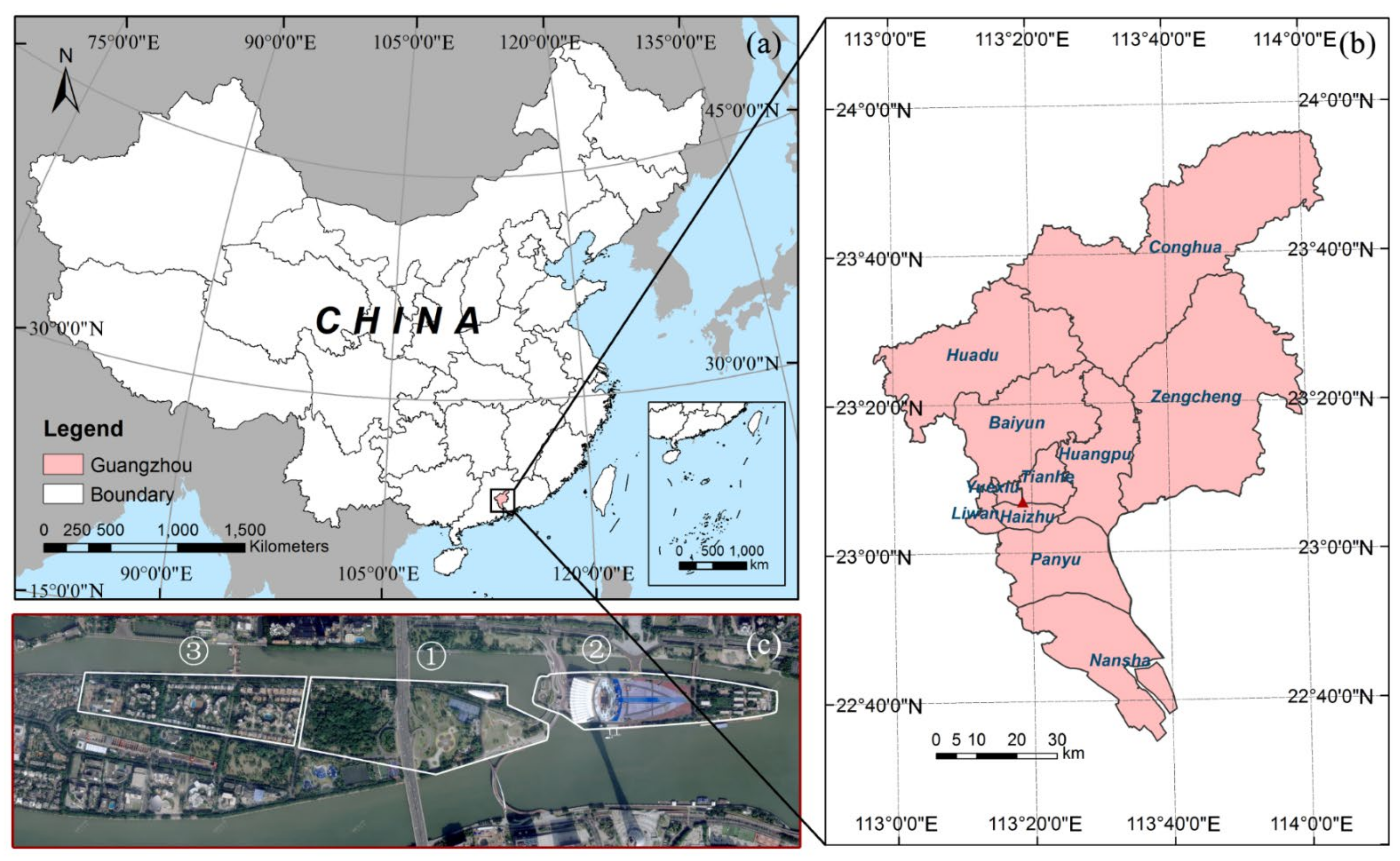
2.1. Study Area

The geographic location and remote sensing images of the study area are shown in Figure 1. Located at the center of Guangzhou’s axle wire, Haixinsha represents an important urban image of the city. The cultural square for citizens, Haixinsha along with Ersha Island, which is positioned as a natural recreational attraction, are popular tourist attractions all year around. As the important landmarks in Guangzhou, the planning of the outdoor environment is particularly important. Not only does the impact on environmental comfort and aesthetics need to be considered but also the regional suitability and economic viability of urban planning. The quality and sustainability of the outdoor environment not only affects the experience of residents and visitors to public spaces but also the regional economic development.
Our study focuses on the city of Guangzhou, China, which is located on the southern coast of China and has a typical tropical monsoon climate. GBA is the most populous of China’s four major bay areas. The region is in the midst of a rapid urbanization process, and the conflict between economic development and the ecological environment is becoming more and more prominent. Therefore, choosing Guangzhou as the study area is beneficial to our understanding of how to build sustainable cities in a region with high environmental protection pressure. The results of this study, as a modelable experience, can be applied to cities with similar climatic conditions and social attributes, and also provide a pilot program for other regions with less pressure to mitigate conservation.
In this study, two adjacent islands, namely, Ersha Island and Haixinsha, were selected. Both are located in the Pearl River Basin of Guangzhou (latitude: 23.1°, longitude: 113.3°). Three functional areas (i.e., a park, a square, and a residential district) from the two islands were selected for this study. Figure 2b shows their exact locations. The classification and proportion of infrastructures for the three functional areas are shown in Table 1.

2.2. Data Collection

2.2.1. Case Study Area and Data for Ecological Benefits

The ENVI-met model can simulate not only the environmental microclimate but also the pollutant concentration variation. Recently, the ENVI-met model has been extensively validated and used in similar studies assessing the environmental benefits of urban infrastructures [14,15,16], demonstrating its reliability and effectiveness for corresponding ecosystem service analysis. In addition, it provides temperature/pollutant concentration distributions horizontally and vertically from 0 to 2500 m in height, which is essential for assessing the air purification and cooling effect of urban infrastructures at a localized level. The three-dimensional data help researchers quantify the cooling/purification effects of blue–green–grey infrastructure and estimate the potential cooling energy-saving/air purification benefits within the modeled area. ENVI-met integrates various environmental factors such as temperature, humidity, wind speed, and direction, as well as the presence of vegetation and building materials. Such a holistic approach is crucial for our research, as it allows us to consider how these factors interact to influence air quality and cooling effect. Furthermore, by adjusting the parameters of different functional area substrates and varying the configuration of the infrastructure in the modeled scene, ENVI-met allowed us to simulate different scenarios of blue–green–grey infrastructure planning. Consequently, spaces with heights equal to or higher than the highest plant/building height were selected for a temperature analysis based on the modeled area [17]. In this study, both the average building height and the highest plant height were approximately 22 m. Therefore, the adjacent grid above 22 m (i.e., 22.5 m) was selected as the upper limit of the vertical range. The data underlying the cooling energy-saving and air purification benefits, temperature, and PM2.5 concentration, accordingly, were obtained with extraction from ENVI-met.
The infrastructure planning scenarios were divided into two categories: “adding” and “replacing” (adding 5% blue, green, or grey infrastructures to the study area or replacing 5% of the green infrastructure with blue or grey, respectively), as shown in Figure 2a. However, due to the dense buildings and the compact distribution of facilities, the adding scenarios were not conducted in the residential district. Therefore, a total of six adding scenarios and six replacing scenarios were performed. In addition to the adding and replacing scenarios, the two were combined to create an integrated environmental planning simulation in the park and square (no overlap between the added or replaced areas), resulting in the overall scenario for the three functional areas. Since no adding scenario was made to the residential district, the integrated scenario was not planned there either. A more thorough description of the study area and model inputs is included in previous work [3].
In urban infrastructure planning, common transformation scenarios include additions, replacements/renewals, reconstruction, intelligentization, and rehabilitation/maintenance. To the operating range permitted by the ENVI-met model, we selected adding and replacing scenarios and also introduced the addition of integrated scenarios. In the finalized 12 scenarios, we provided researchers and urban planners with as many basic and diverse scenarios as possible so that the results could serve as a theoretical reference for engineering practice.

2.2.2. Sources of Cost

The specific types of blue–green–grey infrastructure involved in the planning scenarios (trees, grasslands, pools, fountains, pavilions, and promenades) were divided into green spaces and building facilities to calculate their market construction standard values as well as costs. The construction costs of green spaces, pavilions, trees, and pools under different scenarios were specifically calculated by referring to the “Guangzhou City Housing Construction Engineering Technical and Economic Indicators” issued by the Guangzhou Municipal Housing and Urban–Rural Development Bureau in 2019. The average value of maintenance costs was calculated according to “Estimated Indicators of Routine Maintenance Annual Costs Projects of Urban Green Spaces in Guangzhou city” and “Comprehensive Quotas for Housing Construction and Municipal Repair Works in Guangdong Province”.

2.3. Cost–Benefit Analysis (CBA)

CBA requires calculating all relevant benefits and costs arising from blue–green–grey infrastructure. Currently, there are four main types of ecological benefit measurements [18,19]:
(1)
Revealed preference methods mainly use the travel costs method and the hedonic price method to estimate ecological benefits. The travel costs method is based on the idea that the time and travel cost expenses that people incur to visit a site represent the “ecological value” of access to the site. The hedonic price method involves determining the impact of a particular service on the price of a corresponding market good, typically residential properties. This approach seeks to isolate and quantify the contribution of the service to the overall market value of the property.
(2)
Stated preference methods include the contingent behavior method and the choice modeling method. The contingent behavior method needs researchers to directly ask survey respondents about their willingness to pay for the enhanced benefits brought by public goods and services. Its appeal lies in providing researchers with a direct view of economic decisions associated with the goods in question.
(3)
Market goods methods estimate ecological benefits using the opportunity cost method, the replacement cost method, and the shadow price method. These methods are usually based on direct measurement or statistical data. The opportunity cost method represents the value that could have been derived if the resource had been used in its next best alternative way. For instance, if a piece of forest land is preserved for its biodiversity value instead of being used for logging, the opportunity cost would be the income that could have been generated from logging. The shadow price method is a way of estimating the cost or benefit of an activity or project that is not reflected in the market price. It provides a monetary measure of the economic impact that would occur if the activity or project was implemented.
(4)
RS-GIS-GPS integration technology combined with professional calculation models.

2.3.1. Replacement Cost Method

This research used the replacement cost method, whereby the services provided by the ecosystem can relatively be provided by an artificial system [20]. At this point, the value of ecosystem services equals the cost of the artificial system, as an equal cost must be paid to obtain these services [21]. For example, it can be assumed that if a forest did not exist, a reservoir that holds equivalent water could replace its position. Then, the economic value of the forested water source would be the cost of investment, operation, and management of the reservoir. The difficulty in the replacement cost method is determining reasonable costs of the alternative processes, as the costs vary with different processes and levels of technology.
In our study, we opted for the replacement cost method mainly for two reasons. Firstly, this method is particularly effective when the direct market valuation of ecosystem services is not feasible. It allows us to quantify the ecological benefits by calculating the cost of replacing or restoring the services provided by the ecosystem, which is especially relevant for our study on the ecosystem service of blue–green–grey infrastructure. The replacement cost method was also commonly used in existing case studies to evaluate air purification and heat island mitigation services [22]. Secondly, our research does not involve travel activities, alternative planning of natural resources, or payable services for residents. Therefore, methods such as the travel costs method, opportunity cost method, and stated preferences methods are not applicable in this context.

2.3.2. Screening of Cost and Benefit Calculation Indicators

According to the urban design and construction objectives, determining all the possible costs and benefits indicators is a prerequisite in measuring the total costs or benefits of blue–green–grey infrastructure.
By integrating dense vegetation into urban areas, we can mitigate the urban heat island effect with enhanced cooling processes and the absorption of short-wave radiation. This strategic approach not only regulates the local climate but also elevates the comfort level of the urban environment. Moreover, it reduces the energy required for cooling buildings, which in turn decreases pollutant emissions, contributing to a healthier and more sustainable urban landscape [23]. The amalgamation of blue–green–grey infrastructure is pivotal in enhancing the climate resilience of cities, for instance, when confronted with threats of heat stress and air pollution [11,24]. This strategic blend of infrastructures provides a robust framework for cities to withstand and adapt to environmental challenges, ensuring healthier and more sustainable urban ecosystems. Therefore, the cooling energy-saving benefits and the air purification benefits of blue–green–grey infrastructure were measured in this study.
Guangzhou is located in a subtropical monsoon climate zone with lengthy hot summers and mild winters. According to the Chinese climate definition method in the “Division of Climatic Season (QX/T 152-2012)” [25], the average multi-year start of summer and autumn in Guangzhou is 16 April and 29 October, respectively. Therefore, the city has an average summer of 196 days, which means the warm period accounts for 53.7% of one year. The local winter rarely requires heating; thus, the infrastructures mainly contributed to cooling energy savings during the warm period, according to local research [26]. Therefore, this study chose a representative day during the warm period (15 June 2019) to carry out field measurements. As construction and maintenance costs are not affected by seasonal variation, they were calculated by multiplying the annual average by the percentage of warm periods.

2.3.3. Calculation of Cost and Benefit Indicators

(1)
Cost calculation
The construction and maintenance costs were calculated based on the types of blue–green–grey infrastructure. The adopted infrastructures including trees, grasslands, pools, fountains, pavilions, and promenades were divided into green spaces and built facilities for calculation. The two were summed to obtain the total cost ( C ) for one year under different scenarios, as shown in Equation (1):
C = C A + C B
where
  • C—the total cost;
  • C A —the construction cost;
  • C B —the maintenance cost.
The variation in costs is obtained by the calculated costs of each scenario subtracting the one in a realistic scenario. Such variation equals the extra or reduced cost to plan for the simulated scenarios. The total cost is then averaged over the overall area to obtain the variation in cost ( Δ C ¯ ) per unit of area (m2), which is shown in Equation (2):
Δ C ¯ = Δ C A
where
  • Δ C—the value of variation in cost;
  • 𝐴—the regional area (m2).
(2)
Cooling energy-saving benefits calculation
As the cooling energy-saving effect of blue–green–grey infrastructure is expressed in the outdoor space, the definition of the spatial extent is necessary. Since the area above buildings and vegetation lacks human activity, the highest plant/building height (hmax) is selected as the upper limit for the temperature analysis [17]. This study extracted the daily average temperature at different heights within the study area and subtracted the realistic scenario. The daily average cumulative temperature variation ( T a ) from ground level to height ( h ) was calculated using Equation (3):
T a = 0 h m a x g h f ( h ) d h
where g h and f ( h ) denote the daily average temperature at height ( h ) under the scenario simulations and the realistic scenario, respectively. ∆Ta is then converted into energy consumption variation ( Q , the average daily variation in the energy value), as described in Equation (4):
Q = c m T a = c ρ s 0 h m a x g h f ( h ) d h
where
  • h —the height above ground (m);
  • c —the specific heat capacity (J/kg·°C);
  • m —the air mass (kg);
  • ρ —the air density (kg/m3);
  • s —the size of the study area (excluding built-up areas).
The difference in energy consumption between the scenario simulations and reality can be seen as the variation in air conditioning energy consumption. For the results, the air conditioning energy consumption difference is converted into kW·h units to count electrical energy. By multiplying the energy variation by the electricity price, the cooling energy-saving benefits ( B q ) can be calculated, as shown in in Equation (5):
B q = Q × P q
where Q—the difference in energy consumption for air conditioning (kW·h);
P q —the electricity charge, calculated at 0.086 USD/kW·h in this study. (The detailed meanings of all the units in this study are explained in Table S1).
(3)
Air purification benefit calculation
In the same way, the highest plant/building height (hmax) in the study area is used as the upper limit of the vertical range. We measure the average PM2.5 concentrations at different heights within the spatial extent using the ENVI-met model. Then, we subtract the realistic scenario to obtain the daily variation in the average cumulative PM2.5 concentration (∆PM2.5) from the ground to height h. The calculation is shown in Equation (6):
P M 2.5 = 0 h m a x g h f ( h ) d h
where g h and f ( h ) denote the daily average P M 2.5 concentrations at height h under the simulated scenarios and reality, respectively. The P M 2.5 can be regarded as the variation in pollution concentration (M) in the region. With the replacement cost method, we multiply P M 2.5 by the cost of cleaning equivalent P M 2.5 to obtain the air purification benefit B m [27], as shown in Equation (7):
B m = M × P m
where
  • M—the difference in the amount of pollution (g/m3);
  • P m —the air purification cost.

2.4. Analysis Period

The analysis period is the key variate affecting the CBA; hence, it is essential to rigorously define the analysis period [1,8]. The analysis period is not only the process of comparing costs throughout service life but is also a key point in determining the break-even point of a project. Therefore, the calculation of the period should take into account the properties and usage of the construction. It is generally accepted that the concept of endurance life is related to the life-cycle accounting approach to building design, construction, and management. The optimal expected service life is assigned to each subsystem and installed accordingly.
According to a field survey of eight urban areas in Guangzhou, the average longest lifetime of greenways and woods was 25 and 150 years [28]. In other words, outdated green infrastructure needs to be upgraded if it exceeds that period. Given that CBA encompasses the costs of infrastructure construction and maintenance, it is pivotal to align the simulation duration with the infrastructure’s life cycle. This application enriches the practical relevance of the results in real scenarios. Thus, in this study, 25 years and 150 years were defined as short-term and long-term, respectively, to assess the costs and benefits of blue–green–grey infrastructure over their lifetime.

2.5. Discount Rate and Net Present Value of Benefits

The value of future costs differs from the current one, even if they are of the same nominal value. To address this difference, the discount rate was used. The discount rate is an interest rate used to convert future cash flows into current values. It reflects the effect of time on the value of money. The higher the discount rate, the lower the value of future cash flows as they appear today. The discount rate, also called the interest rate, is often used to determine the present value of future cash flows in a discounted cash flow analysis. Interest rates can be divided into a nominal discount rate (which does not consider inflation) and a real discount rate (which includes inflation).
Here, we discounted the maintenance costs and ecological benefits to the initial investing year within the whole service life. Referring to the “Construction Projects Economic Evaluation Method and Parameter (third edition)” issued in China and the recommended values in recent research [29], a discount rate of 6% was used. In our study, the discount rate allowed us to compare costs and benefits occurring at different points in time on a common footing. It is important to note that a higher discount rate would reduce the present value of future benefits, making projects with long-term benefits less attractive. Conversely, a lower discount rate would increase the present value of future benefits. Thus, the choice of discount rate will impact the results of our cost–benefit analysis. However, we believe that 6% is a reasonable and commonly accepted average rate for relevant studies in China.
The Net Present Value (NPV) measures a project’s financial benefit by discounting all resulting cash flows (at a certain internal rate of return) to the project’s start time. Therefore, NPV can be viewed as the “cash equivalent” of executing the project [30]. With the introduction of the discount rate, the NPV of the ecological benefits of the blue–green–grey infrastructure can be calculated, as shown in Equation (8):
N P V = t = 1 n B t C B t 1 + k t C A
where
  • n —the life span of the construction project (year);
  • t —the time when the cash flow occurs (year);
  • k —the discount rate (%);
  • B t —the ecological benefits in year t ;
  • C B t —the maintenance cost in year t ;
  • C A —the construction cost.

3. Results and Discussion

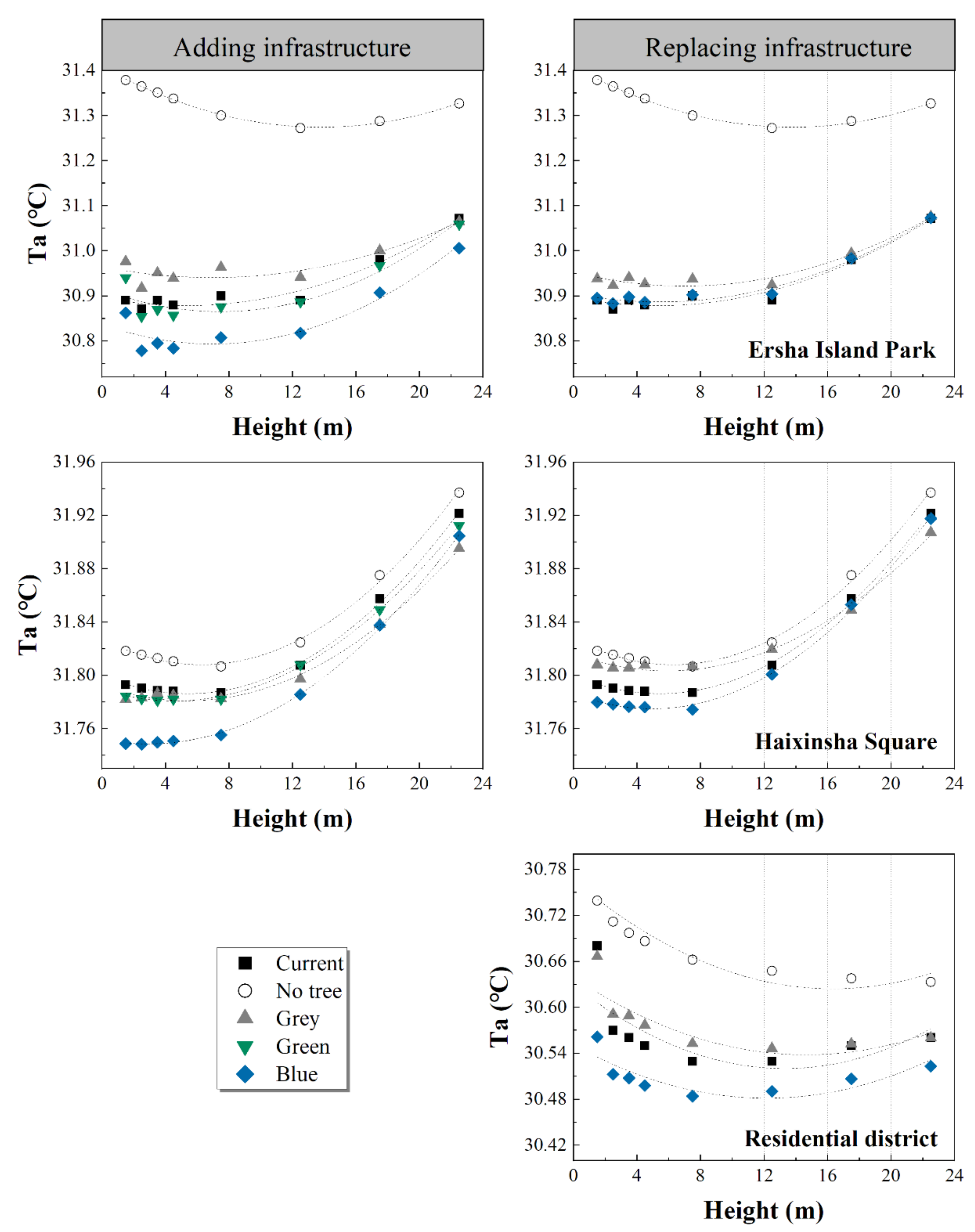
3.1. Cooling Energy-Saving Benefits under Different Scenarios

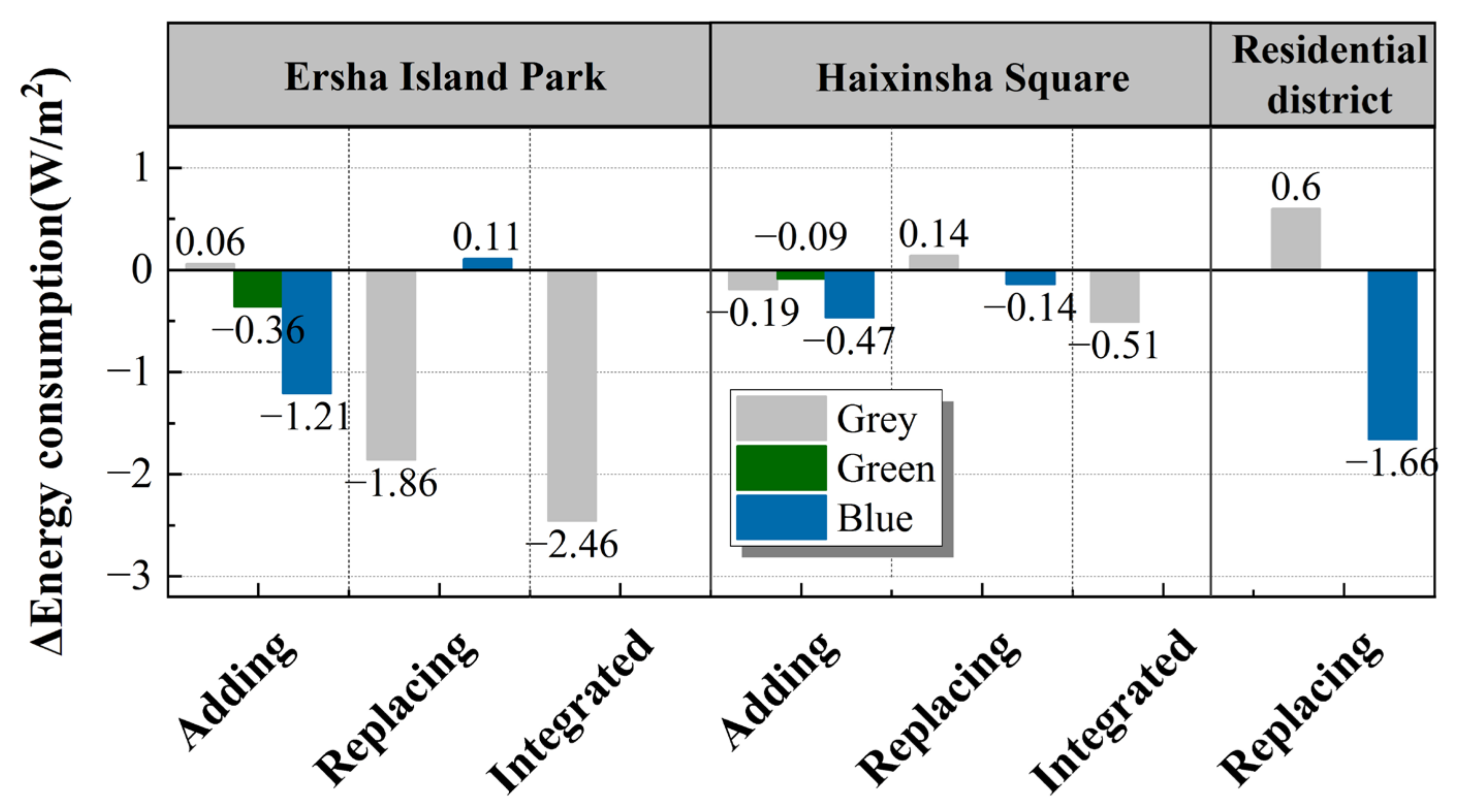
3.1.1. Comparison of Energy Variation

The overall average temperature at different heights was extracted using the ENVI-met model. The trend in temperature variation with height is demonstrated in Figure 3.
As shown in Figure 3, the temperature increased with height in the park and the square. For the residential district, there was an initial decrease followed by a slow increase. The residential district in the study area had more trees than the other two sites, which probably led to the initial decrease in temperature. The subsequent increase was probably caused by the sparser trees and less shade as the height increased [31,32]. Furthermore, by comparing the three types of infrastructures, it was found that the temperatures were always the minimum when both adding and replacing blue infrastructure. In other words, the blue infrastructure showed the most outstanding cooling effect among all functional areas in different scenarios. This might be because the blue infrastructure was effective in reducing ambient temperatures through the evaporation and convection of water [33,34,35]. Urban water bodies such as reservoirs, lakes, and rivers, with their inherent high thermal capacity and fluidity, could play an important role in mitigating the urban heat island effect [36]. Saaroni et al., also found that even small water bodies had a cooling effect under both dry and hot and humid conditions within a distance of approximately 40 m [31]. Table 2 shows the multiple nonlinear regression equations between temperature and height under different scenarios.
The integral operation from the fitted equations gave the energy variation over the whole space (Figure 4). The actual situation was subtracted from the results to obtain the average daily energy variation for each scenario. If a positive value was obtained, representing an increase in temperature, it brought a negative cooling energy-saving effect, and vice versa. The formula (Table 2) might be more applicable to subtropical climates in the summer.
The energy consumption in most adding scenarios was significantly reduced compared with reality, demonstrating a positive cooling energy-saving effect (Figure 4). Blue infrastructure had the most significant cooling effect in both the park and square, with an average daily cooling energy savings of 1.21 W/m2 and 0.47 W/m2. This was consistent with the results of previous studies. Su et al., studied 17 parks in Guangzhou and found that parks with a larger proportion of water bodies had greater thermal mitigation capacity than parks with smaller water bodies [37]. The reason why the cooling capacity of adding blue infrastructure in the park was stronger than that in the square might be the configuration of the water body. Sun et al., found that the landscape shape index of a wetland had a negative correlation with cooling intensity, which meant a circular-shaped wetland performed better than an elongated one [38].
However, the results in the replacing scenarios were more functionally characterized by variability (Figure 4). For the park, while adding grey infrastructure slightly increased energy consumption, replacing 5% of the green with grey infrastructure resulted in significant cooling energy savings. Replacing the infrastructure with blue, on the other hand, increased the temperature and resulted in negative energy savings. It was worth noting that the integrated scenario (i.e., adding 5% grey infrastructure and replacing 5% of the green with grey infrastructure) performed the best in terms of energy savings, with an average daily energy consumption reduction of 2.46 W/m2. The results demonstrated that for parks with abundant green infrastructure, the combination of grey and green infrastructures not only improved human thermal comfort but also saved energy. Some studies have found that combinations of different parameters created special synergies and provided better mitigation. For example, in a park in Beijing, it was observed that the combination of trees and gazebos was much better than solitary structures [39].
For squares, replacing some of the green infrastructure with grey infrastructure slightly increased the temperature. However, the highest cooling energy savings were obtained when combined with adding more grey infrastructure. This might be because for squares with large fountains, promoting the circulation of water vapor in the water body is an important factor in determining the local microclimate [40]. Buildings such as semi-enclosed pavilions with adequate ventilation can effectively promote airflow and provide stable shade for reducing direct sunlight on the water body. Thus, they could reduce the temperature of the water body and allow it to better absorb ambient heat, resulting in a cooling and energy-saving effect.
For the residential district, replacing 5% of the green with blue infrastructure reduced the overall density, and the evaporation of water promoted heat dissipation. Such a scenario effectively reduced temperatures and saved cooling energy by 1.66 W/m2. Outdoor artificial water bodies, such as fountains and pools, could reduce ambient temperature by evaporating water and dissipating heat, thus saving energy [41]. Studies on the cooling effect of blue infrastructure have been reported in many regions. A study found a positive effect of river evaporation on reducing urban temperatures in London [42]. The results were also related to the functional characteristics of the specific region. Liu et al., explored the relationship between microclimatic factors and residents’ activities within landscape gardening areas in the urban residential district of Shanghai [43]. They found residents preferred the waterfront as a resting place during lunchtime hours, which was considered to be more comfortable [43].

3.1.2. Comparison of Cooling Energy-Saving Benefits

The energy efficiency under different scenarios was converted into cooling energy savings using the replacement cost method. Figure 5 shows the ecological benefits per square meter by converting cooling energy savings into an equivalent amount of electricity. The annual average energy savings for the three sites under different scenarios were first compared regardless of seasonal differences in benefits. By screening the planning scenarios for optimal cooling energy savings, we found that the best scenarios differed for different functional areas. For the park, adding blue infrastructure and replacing green with grey infrastructure resulted in favorable cooling energy savings, with benefits augmented by 0.91 USD/m2/yr and 1.39 USD/m2/yr, respectively. Moreover, the integrated scenario resulted in the greatest cooling energy-saving benefit of 1.98 USD/m2/yr. In terms of the square, the integrated scenario also resulted in the highest cooling energy savings, with an annual benefit addition of 0.38 USD/m2. For the residential district, replacing green with blue infrastructure provided the best cooling energy savings. The combination of blue and grey infrastructure yielded an annual benefit of 1.24 USD/m2. A plausible reason could be that the dense building shadows were effective in blocking out sunlight [44] and the cooling effect of evaporating water from blue infrastructure reduced the surrounding temperatures.

3.2. Air Purification Benefits under Different Scenarios

3.2.1. Comparison of Air Purification Effectiveness

Figure 6 shows the annual average variation in PM2.5 concentrations, and it indicates that the changes in infrastructure had the greatest impact on the park. The variation in PM2.5 concentrations was almost ten times greater than the other two sites with the same proportion of addition or replacement. The reason might be that the park was adjacent to a major traffic artery to the west, which had a higher traffic flow than the other two sites. Vehicle exhaust was the main source of pollutants, so the concentration of particulate pollutants was higher, and the change range was greater. The results of atmospheric monitoring experiments conducted by Wang et al. [45] showed that the closer the road, the greater the impact on PM2.5 concentrations.
In addition to the adding and replacing scenarios, the two were combined to create a holistic environmental planning simulation, obtaining an integrated scenario. It is also worth noting that the residential area was too densely built for the adding scenario, and the replacing scenario gave good results in terms of air purification and energy efficiency. Therefore, no further integrated scenarios were planned in this area.
Based on the comparison of air pollution reduction effectiveness (Figure 5), the integrated scenario could effectively clean the air with a reduction in PM2.5 concentration of 3.6 μg/m3 in the park and 0.56 μg/m3 in the square. A subsequent comparison of the PM2.5 concentrations at different heights in the integrated scenario is sown in Figure 7. There was a significant reduction in PM2.5 concentrations at different heights when comparing the integrated scenario with the realistic situation. In the park, a maximum reduction of 22 μg/m3 (at 1.5 m) was achieved. The PM2.5 concentration also decreased with increasing height. Song summarized the dispersion pattern of inhalable particles in the vertical direction, where the concentration of pollutants decreased with increasing height [46]. The results of Viecco et al., showed that green roofs were effective in reducing PM2.5 concentrations at building heights of 5 m and 10 m [14]. However, they failed to improve air quality at pedestrian levels at building heights of 20 m and 30 m. In this study, the air purification effect of the infrastructures also decreased with increasing height, which was probably caused by the lower density of vegetation at higher heights. The main purification effect occurred below 12.5 m, which was the main area of human activity in the park and square. Overall, the results were consistent with the study by Viecco, Jorquera, Sharma, Bustamante, Fernando, and Vera [14].
To sum up, there was a significant reduction in air pollution under the integrated design scenario, bringing considerable air purification benefits. The air environment in the park and square was effectively improved and was of reference for practical planning.

3.2.2. Comparison of Purification Benefits

By extracting the pollutant concentrations and with the relationship between concentration and height, the pollutant concentrations in the height space of the buildings were calculated. Subsequently, the value was averaged over the whole area. Then, it was subtracted from the realistic scenario to obtain the air purification effect under different scenarios without considering seasonal differences. The results are shown in Figure 5.
The results show that both blue and grey infrastructures had a certain effect on PM2.5 purification. Blue infrastructure removed dust by increasing air humidity. A study by Zhu et al. [47] showed that when the area of urban lake wetlands increased, the humidifying effect gradually strengthened and the PM2.5 and PM10 concentrations decreased. When the area of lake wetlands reached a certain value, the lake wetlands promoted surrounding cool and warm airflow. This made the dust particles in the air more easily disperse in the direction of lower humidity, thus improving the air quality in wetlands. The air pollution reduction effect of grey infrastructure was more pronounced. The result suggested that semi-enclosed grey infrastructure like gazebos were instead less likely to trap airborne pollutant particles through a certain layout. Previous research showed that vegetated surfaces trap thirty times more particulate pollution than smooth concrete surfaces [48]. However, adding more green infrastructure also increases the adsorption of particulate matter and impedes air circulation [49], exacerbating air pollution [50]. Therefore, a higher proportion of green infrastructure is not always a better choice. Tree stand density, leaf area density, and tree canopy bottom height need to be taken into account to avoid the weakening of the dispersion effect brought by porous vegetated barriers [51].
Figure 5 also shows that the air purification benefits were greatest for the park in the scenario with 5% grey infrastructure added, obtaining 15.22 × 10⁻³ USD/m2/yr. For the square, the integrated scenario had the greatest increase in annual benefits, being 2.46 × 10⁻³ USD/m2/yr. For the residential district, replacing green with grey infrastructure showed the best air pollution reduction effect, with a gain of 0.29 × 10⁻³ USD/m2/yr. Thus, it can be seen that grey infrastructure was most effective in purifying the park, square, and residential districts because most of the areas added and replaced infrastructures were in the upwind direction (southeast wind, wind direction 135°). Buildings such as semi-enclosed permeable gazebos could help airflow and reduce pollutant concentrations. Wu et al., concluded that the distribution of PM2.5 concentrations in residential districts with different layouts differed significantly [52].
Overall, the ecological benefits showed positive variation under most scenarios (Figure 5), while the changing value of cost (provided in Table S2) also needed to be considered for estimating the feasibility further.

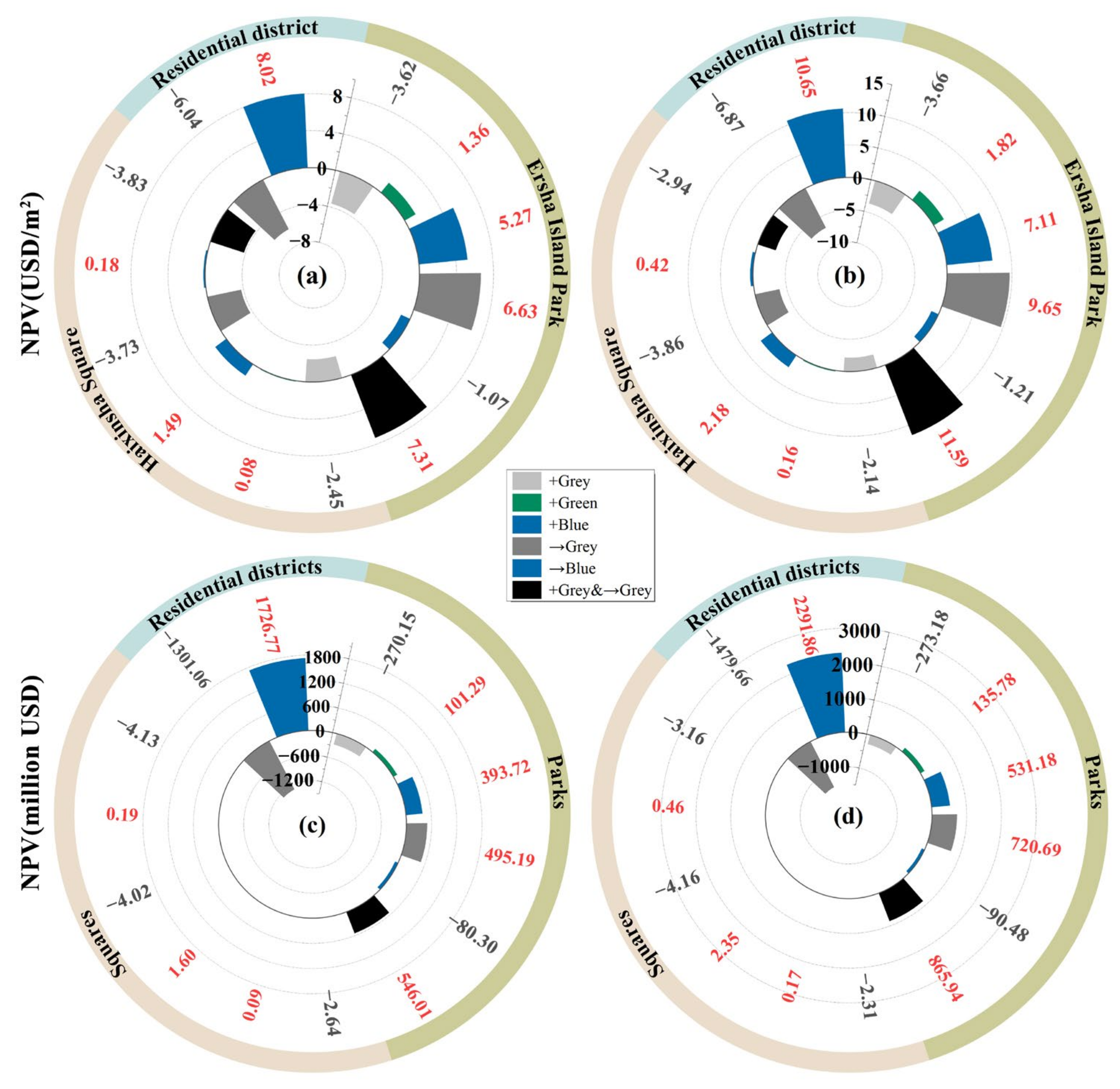
3.3. Trade-Offs under Different Scenarios

3.3.1. Temporal-Scale Scenarios

The total costs and benefits were combined to obtain the total NPV of ecological benefits under different scenarios. The seasonal differences in benefits were taken into account in this step. The results are shown in the form of the short-term life span (25 years, Figure 8a) and the long-term life span (150 years, Figure 8b) during warm periods. If the value was negative, the scenario was not only costly but also harmful to the environment. Conversely, if the value was positive, it had a positive ecological benefit to some extent and improved the environmental quality.
In Figure 5, it can be seen that both adding and replacing the blue–green–grey infrastructure yielded much stronger cooling energy savings than purification benefits. This suggested that cooling energy savings played a decisive role in the CBA. Field measurements in Guangzhou also found that urban green spaces had a more significant effect on heat regulation than air purification [53]. The positive and negative trends in the NPV of ecological benefits were consistent for the short term and the long term during warm periods, with the latter yielding greater absolute values.
For the park, adding green or blue infrastructures, replacing some of the green with grey infrastructure, and the integrated scenario all yielded positive NPV of ecological benefits. The highest effect was achieved with the integrated scenario at 7.31 USD/m2 in the short term and 11.59 USD/m2 in the long term. The NPV turned positive after eight years of operation to recover costs. At this point, the two ecological benefits were the highest among all scenarios for the park.
For the square, the NPV obtained by adding more blue infrastructure was the highest, at 1.49 USD/m2 for the short term and 2.18 USD/m2 for the long term, respectively. The cost could be recovered after operating for six years. However, for squares with a large area of blue infrastructure originally, the expansion of the area of blue infrastructure needed to further consider the actual needs and feasibility. On the premise of considering the balance of the blue–green–grey infrastructure ratio and ecosystem stability, it was recommended to choose the option of adding green infrastructure, which could also achieve a positive NPV.
For the residential area, replacing part of the green infrastructure with grey or blue infrastructure gave very different results. The NPV reached −6.87 USD/m2 and 10.65 USD/m2, respectively, for the long term. The results suggested that it was not advisable to expand the buildings in the residential district. Meanwhile, the proportion of green infrastructure should be maintained to preserve the local ecological function. If some of the green was replaced with blue infrastructure, a positive NPV could be achieved after one year of operation. The water landscape could regulate temperature, purify the air, and improve the microclimate in residential districts [54]. Therefore, for the residential district, adding more blue infrastructure could improve the quality of the environment and ecology. This also provided a theoretical basis for the feasibility and necessity of planning blue infrastructure such as pools and fountains in residential districts.
Based on the results in Figure 8, we weighed up the scenarios for each functional area to achieve the best NPV. All the scenarios could recover costs in a relatively short period of operation. In addition, it was helpful to conduct a more comprehensive CBA analysis by considering as many infrastructure-related costs and environmental benefits as possible [55]. For some scenarios with a negative NPV, it might result from excluding the cool period or calculating too few types of ecological benefits. If more ecological benefits such as CO2 absorption, a reduction in surface runoff, or social and economic benefits were included, a different result might be achieved. When multiple ecological benefits were introduced, it was necessary to consider the characteristics and needs of the functional areas and seek to maximize the synergy between multiple functions [56].

3.3.2. Spatial-Scale Scenarios

According to the statistics from the “Guangzhou City Master Plan” issued in 2018, it is known that the total area of Guangzhou’s parks, squares, and residential districts is 7.47 × 10⁷ m2, 1.08 × 10⁶ m2, and 2.15 × 10⁸ m2, respectively. Finally, a CBA of the overall infrastructure planning in Guangzhou was carried out based on the total NPV of ecological benefits per unit area. Figure 8 shows an assessment of the environmental impact of optimizing blue–green–grey infrastructure at the urban scale during warm periods. The results showed that the integrated scenario in Guangzhou’s parks achieved the highest NPV. The NPV reached 546.01 million USD/25y in the short term (Figure 8c) and 865.94 million USD/150y in the long term (Figure 8d). For the square, the highest NPV was obtained with the inclusion of 5% blue infrastructure. The highest NPV (2291.86 million USD/150y) could be achieved in the long term if 5% of the green infrastructure was replaced with blue infrastructure in residential districts.

3.4. Implications for Urban Planning

The findings of this study suggested that the economic benefits of optimizing the configuration of infrastructure aiming at the characteristics of different functional areas were considerable in urban planning. The same type of infrastructure performed differently in different functional areas and also on different ecosystem services. However, in particular, grey infrastructure showed excellent air pollution reduction capacity in all functional areas due to its dispersion effect on the urban environment. Therefore, in the design of sustainable cities, the configuration and addition of blue–green infrastructure, as well as the combination of grey infrastructure with them, are equally important. These infrastructures can produce the maximum comprehensive ecological benefits according to local conditions only when people make full use of the ventilation and heat dissipation capacity of constructions. Specifically, we can appropriately add pavilions and promenades in parks, enlarge the area of artificial lakes and rivers in squares, and build fountains and swimming pools in residential districts, which can improve the ecosystem service benefits of the original blue–green–grey infrastructure. By comparing the two ecological service benefits in the same scenario, it could be seen that the cooling energy-saving benefits were more pronounced than the air purification benefits, reaching a difference of several times to several hundred times. The phenomenon suggests to us that it is necessary to identify the most influential one when evaluating the ecosystem service benefits of infrastructures in a certain region, which is related to the climatic conditions and regional environment in the study area. For example, the heat mitigation effect of trees was noteworthy during the warm period while it was small during the cool period [17]. Because the contribution of a certain service might be predominant, such identification is further effective for the trade-offs in land use and resource allocation, which is similar to the use of the Ecosystem Service Value Database established by de Groot et al. [10].

4. Conclusions

In this research, the environmental benefits under different blue–green–grey infrastructure plans were monetized from an economic perspective, incorporating costs to explore the applicability of different planning scenarios. The replacement cost method was used here to assess the environmental benefits of urban infrastructures under different scenarios. While this study only measured cooling energy-saving and air purification benefits, the total environmental benefits were relatively high. We found that the integrated scenarios (adding 5% grey infrastructure and replacing 5% of the green with grey infrastructure) resulted in the best cooling energy savings for parks and squares and that increasing the proportion of blue infrastructure contributed more to heat mitigation in the residential district. As for air purification benefits, adding 5% grey infrastructure in parks, implementing integrated scenarios in squares, and replacing 5% of the green infrastructure with grey infrastructure in the residential district became the optimal scenarios, respectively.
By comparing the NPV of the ecological benefits under different scenarios during warm periods, it was concluded that the optimal planning scenarios for different functional areas differed. A long-term project generally yielded higher benefits than a short-term one. Adding 5% grey infrastructure and replacing 5% of the green with grey infrastructure was the best option for parks and would pay for itself after operating for eight years, which not only reduced the ambient temperature and provided significant cooling energy savings but also provided a high level of air purification benefits. At the urban scale, the NPV was USD 546.01 million in the short-term life span and USD 865.94 million in the long-term life span. For squares, the highest NPV was obtained by further adding 5% blue infrastructure, while for a square with a large water area, the feasibility needed to be analyzed in combination with other ecological benefits. Finally, for the residential district, replacing the 5% of the green with blue infrastructure, with only warm periods benefits calculated, resulted in a total NPV after just one year of operation, and a return of USD 1726.77 million in the short-term life span, which was the most competitive among all scenarios.
Considering the shortcomings of this study, we suggest that future studies could involve more ecological benefits of blue–green–grey infrastructure, such as water retention, carbon sequestration, oxygen absorption, and their synergies. The benefits during the cool period could also be included to make the CBA more comprehensive. In addition, exploring more combinations of blue–green–grey infrastructure is an effective means of building climate-resilient cities. For example, rainwater harvesting tanks and rain gardens can be used as a combination of blue–green infrastructure, and green roofs and buildings with high albedo materials can be applied as a combination of green–grey infrastructure. Further research could also be conducted on the improvement in the spatial configuration of different types of infrastructures, rather than just changing the proportional configuration.
By conducting cost–benefit analyses of 12 scenarios in Guangzhou City, our study obtained the optimal blue, green, and grey infrastructure retrofitting scenarios applicable to three functional areas (a park, a square, and a residential district). This study’s results were analyzed using detailed accounting and comparison, providing quantifiable evidence for optimizing the ecological and economic values of urban infrastructures and offering valuable insights for urban planning stakeholders.

Supplementary Materials

The following supporting information can be downloaded at: https://www.mdpi.com/article/10.3390/su16010203/s1, Text S1: Cost input analysis of blue–green–grey infrastructure; Table S1: Units in this study and the corresponding interpretations; Table S2: Cost input per unit area under different planning scenarios.

Author Contributions

Methodology, Y.W.; Software, J.L.; Formal analysis, H.C. and J.L.; Writing—original draft, H.C. and J.L.; Writing—review & editing, Y.W.; Visualization, H.C.; Supervision, Z.N. and B.X.; Project administration, B.X.; Funding acquisition, Y.W. and Z.N. All authors have read and agreed to the published version of the manuscript.

Funding

This research was supported by [the National Key R&D Program of China] grant number [2022YFE0116300], [the National Natural Science Foundation of China] grant number [42177208], and [the Natural Science Foundation of Guangdong Province] grant number [2019A1515011580, 2022A1515011929]. The APC was funded by [the National Key R&D Program of China] grant number [2022YFE0116300].

Data Availability Statement

The data presented in this study are available on request from the corresponding author. The data are not publicly available due to research privacy.

Conflicts of Interest

The authors declare no conflict of interest.

References

  1. Vojinovic, Z. Flood Risk: The Holistic Perspective, from Integrated to Interactive Planning for Flood Resilience; IWA Publishing: London, UK, 2015. [Google Scholar]
  2. Droste, N.; Meya, J.N. Ecosystem services in infrastructure planning—A case study of the projected deepening of the Lower Weser river in Germany. J. Environ. Plann. Manag. 2017, 60, 231–248. [Google Scholar] [CrossRef]
  3. Li, J.; Wang, Y.F.; Ni, Z.B.; Chen, S.Q.; Xia, B.C. An integrated strategy to improve the microclimate regulation of green-blue-grey infrastructures in specific urban forms. J. Clean. Prod. 2020, 271, 122555. [Google Scholar] [CrossRef]
  4. Wild, T.C.; Henneberry, J.; Gill, L. Comprehending the multiple ‘values’ of green infrastructure—Valuing nature-based solutions for urban water management from multiple perspectives. Environ. Res. 2017, 158, 179–187. [Google Scholar] [CrossRef] [PubMed]
  5. Jonkman, S.N.; Brinkhuis-Jak, M.; Kok, M.; Holterman, S.R. Cost benefit analysis and flood damage mitigation in the Netherlands. In Proceedings of the 14th European Safety and Reliability Conference, Tri City, Poland, 27–30 June 2005; pp. 1179–1187. [Google Scholar]
  6. Engström, R.; Howells, M.; Mörtberg, U.; Destouni, G. Multi-functionality of nature-based and other urban sustainability solutions: New York City study. Land Degrad. Dev. 2018, 29, 3653–3662. [Google Scholar] [CrossRef]
  7. Foster, J.; Lowe, A.; Winkelman, S. The Value of Green Infrastructure for Urban Climate Adaptation; The Centre For Clean Air Policy: Washington, DC, USA, 2011. [Google Scholar]
  8. Vincent, S.U.; Radhakrishnan, M.; Hayde, L.; Pathirana, A. Enhancing the economic value of large investments in sustainable drainage systems (SuDS) through inclusion of ecosystems services benefits. Water 2017, 9, 841. [Google Scholar] [CrossRef]
  9. Ossa-Moreno, J.; Smith, K.M.; Mijic, A. Economic analysis of wider benefits to facilitate SuDS uptake in London, UK. Sustain. Cities Soc. 2017, 28, 411–419. [Google Scholar] [CrossRef]
  10. De Groot, R.S.; Brander, L.; Van der Ploeg, S.; Costanza, R.; Bernard, F.; Braat, L.; Christie, M.; Crossman, N. Global estimates of the value of ecosystems and their services in monetary units. Ecosyst. Serv. 2012, 1, 50–61. [Google Scholar] [CrossRef]
  11. Alves, A.; Gersonius, B.; Kapelan, Z.; Vojinovic, Z.; Sanchez, A. Assessing the Co-Benefits of green-blue-grey infrastructure for sustainable urban flood risk management. J. Environ. Manag. 2019, 239, 244–254. [Google Scholar] [CrossRef]
  12. Getzner, M.; Gutheil-Knopp-Kirchwald, G.; Kreimer, E.; Kirchmeir, H.; Huber, M. Gravitational natural hazards: Valuing the protective function of Alpine forests. For. Policy Econ. 2017, 80, 150–159. [Google Scholar] [CrossRef]
  13. Liu, W.; Chen, W.; Feng, Q.; Peng, C.; Kang, P. Cost-Benefit Analysis of Green Infrastructures on Community Stormwater Reduction and Utilization: A Case of Beijing, China. Environ. Manag. 2016, 58, 1015–1026. [Google Scholar] [CrossRef]
  14. Viecco, M.; Jorquera, H.; Sharma, A.; Bustamante, W.; Fernando, H.J.S.; Vera, S. Green roofs and green walls layouts for improved urban air quality by mitigating particulate matter. Build. Environ. 2021, 204, 108120. [Google Scholar] [CrossRef]
  15. Rui, L.; Buccolieri, R.; Gao, Z.; Gatto, E.; Ding, W. Study of the effect of green quantity and structure on thermal comfort and air quality in an urban-like residential district by ENVI-met modelling. Build. Simul. 2019, 12, 183–194. [Google Scholar] [CrossRef]
  16. Salata, F.; Golasi, I.; de Lieto Vollaro, R.; de Lieto Vollaro, A. Urban microclimate and outdoor thermal comfort. A proper procedure to fit ENVI-met simulation outputs to experimental data. Sustain. Cities Soc. 2016, 26, 318–343. [Google Scholar] [CrossRef]
  17. Wang, Y.F.; Ni, Z.B.; Chen, S.Q.; Xia, B.C. Microclimate regulation and energy saving potential from different urban green infrastructures in a subtropical city. J. Clean. Prod. 2019, 226, 913–927. [Google Scholar] [CrossRef]
  18. Wang, Y.; Li, J.; Wang, H.R.; Ding, X.W.; Cao, X.M. Calculation on compensation value of urban green lands for. J. Beijing Norm. Univ. (Nat. Sci.) 2005, 41, 641–645. [Google Scholar]
  19. Jiang, H.Y.; Xie, D.X.; Zhou, C.S. Quantitative evaluation methods and their practices on the externality of urban green space. Chin. Landsc. Archit. 2010, 26, 78–81. [Google Scholar]
  20. Bockstael, N.E.; Freeman, A.M.; Kopp, R.J.; Portney, P.R.; Smith, V.K. On measuring economic values for nature. Environ. Sci. Technol. 2000, 34, 1384–1389. [Google Scholar] [CrossRef]
  21. Notaro, S.; Paletto, A. The economic valuation of natural hazards in mountain forests: An approach based on the replacement cost method. J. For. Econ. 2012, 18, 318–328. [Google Scholar] [CrossRef]
  22. Croci, E.; Lucchitta, B.; Penati, T. Valuing Ecosystem Services at the Urban Level: A Critical Review. Sustainability 2021, 13, 1129. [Google Scholar] [CrossRef]
  23. Kleerekoper, L.; van Esch, M.; Salcedo, T.B. How to make a city climate-proof, addressing the urban heat island effect. Resour. Conserv. Recycl. 2012, 64, 30–38. [Google Scholar] [CrossRef]
  24. Commission, E. The Multifunctionality of Green Infrastructure; European Commission: Bristol, UK, 2012. [Google Scholar]
  25. QX/T 152-2012; Definition of Climate Season. China Meteorological Press: Beijing, China, 2012.
  26. Wang, Y.; Ni, Z.; Hu, M.; Li, J.; Wang, Y.; Lu, Z.; Chen, S.; Xia, B. Environmental performances and energy efficiencies of various urban green infrastructures: A life-cycle assessment. J. Clean. Prod. 2020, 248, 119244. [Google Scholar] [CrossRef]
  27. Tu, K.H. Quantitative Analysis and Evaluation of Ecosystem Services of Shelter Forest in Ningbo; East China Normal University: Shanghai, China, 2015. [Google Scholar]
  28. Jim, C.Y. Evaluation of Heritage Trees for Conservation and Management in Guangzhou City (China). Environ. Manag. 2004, 33, 74–86. [Google Scholar] [CrossRef] [PubMed]
  29. Shi, F.W. Measurement and Application Suggestions on Social Discount Rate in China. Eng. Econ. 2019, 29, 77–80. [Google Scholar] [CrossRef]
  30. Wiesemann, W.; Kuhn, D.; Rustem, B. Maximizing the net present value of a project under uncertainty. Eur. J. Oper. Res. 2010, 202, 356–367. [Google Scholar] [CrossRef]
  31. Saaroni, H.; Ziv, B. The impact of a small lake on heat stress in a Mediterranean urban park: The case of Tel Aviv, Israel. Int. J. Biometeorol. 2003, 47, 156–165. [Google Scholar] [CrossRef] [PubMed]
  32. Lahmer, W.; Pfutzner, B.; Becker, A. Assessment of land use and climate change impacts on the mesoscale. In Proceedings of the 25th General Assembly of the European-Geophysical-Society, Nice, France, 25–30 April 2021; pp. 565–575. [Google Scholar]
  33. Jacobs, C.; Klok, L.; Bruse, M.; Cortesao, J.; Lenzholzer, S.; Kluck, J. Are urban water bodies really cooling? Urban Clim. 2020, 32, 100607. [Google Scholar] [CrossRef]
  34. Albdour, M.S.; Baranyai, B. Water body effect on microclimate in summertime: A case study from Pécs. Pollack Period. 2019, 14, 131–140. [Google Scholar] [CrossRef]
  35. Bansal, P.K.; Xie, G. A unified empirical correlation for evaporation of water at low air velocities. Int. Commun. Heat Mass Transf. 1998, 25, 183–190. [Google Scholar] [CrossRef]
  36. Jacobs, A.F.G.; Jetten, T.H.; DorothéC, L.; Heusinkveld, B.G.; Nieveen, J.P. Diurnal temperature fluctuations in a natural shallow water body. Agric. For. Meteorol. 1997, 88, 269–277. [Google Scholar] [CrossRef]
  37. Su, Y.X.; Huang, G.Q.; Chen, X.Z.; Chen, S.S. The cooling effect of Guangzhou City parks to surrounding environments. Acta Ecol. Sin. 2010, 30, 4905–4918. [Google Scholar]
  38. Sun, R.H.; Chen, A.L.; Chen, L.D.; Lü, Y. Cooling effects of wetlands in an urban region: The case of Beijing. Ecol. Indic. 2012, 20, 57–64. [Google Scholar] [CrossRef]
  39. Xu, X.Y.; Sun, S.B.; Liu, W.; Garcia, E.H.; He, L.; Cai, Q.; Xu, S.J.; Wang, J.J.; Zhu, J.N. The cooling and energy saving effect of landscape design parameters of urban park in summer: A case of Beijing, China. Energy Build. 2017, 149, 91–100. [Google Scholar] [CrossRef]
  40. Chen, M. The Actual Measurement of Xi’an Urban Outdoor Public Space’s Microclimate Effects Formed in Water—Using the Ci en Temple Area’s Surroundings as an Example; Xi’an University of Architecture and Technology: Xi’an, China, 2015. [Google Scholar]
  41. Yahia, M.W.; Johansson, E. Evaluating the behaviour of different thermal indices by investigating various outdoor urban environments in the hot dry city of Damascus, Syria. Int. J. Biometeorol. 2013, 57, 615–630. [Google Scholar] [CrossRef] [PubMed]
  42. Maas, J.; Verheij, R.A.; Groenewegen, P.P.; de Vries, S.; Spreeuwenberg, P. Green space, urbanity, and health: How strong is the relation? J. Epidemiol. Community Health 2006, 60, 587–592. [Google Scholar] [CrossRef] [PubMed]
  43. Liu, B.Y.; Mei, Y.; Kuang, W. Experimental research on correlation between microclimate element and human behavior and perception of residential landscape space in shanghai. Chin. Landsc. Archit. 2016, 32, 5–9. [Google Scholar]
  44. Yahia, M.W.; Johansson, E. Landscape interventions in improving thermal comfort in the hot dry city of Damascus, Syria—The example of residential spaces with detached buildings. Landsc. Urban Plann. 2014, 125, 1–16. [Google Scholar] [CrossRef]
  45. Wang, T.; Wang, G.X.; Zhou, M.P.; Chen, M.P.; Li, J.; Wu, S.J.; Luo, M. Study on influence factors of PM2.5 concentrations in road region. Environ. Pollut. Control 2016, 38, 25–31. [Google Scholar]
  46. Song, D. Effects of Arbors in Campus Courtyard on Air Flow Field and PM2.5 Pollution Distribution-Take Shenyang Architectural University as an Example; Shenyang Architectural University: Shenyang, China, 2019. [Google Scholar]
  47. Zhu, C.Y.; Zeng, Y.Z.; Chen, Y.R.; Guo, H.J. Effects of urban lake wetland on air PM10 and PM2.5 concentration—A case study of Wuhan. Chin. Landsc. Archit. 2016, 32, 88–93. [Google Scholar]
  48. Mitchell, R.; Maher, B.A.; Kinnersley, R. Rates of particulate pollution deposition onto leaf surfaces: Temporal and inter-species magnetic analyses. Environ. Pollut. 2010, 158, 1472–1478. [Google Scholar] [CrossRef]
  49. Xing, Y.; Brimblecombe, P.; Wang, S.F.; Zhang, H. Tree distribution, morphology and modelled air pollution in urban parks of Hong Kong. J. Environ. Manag. 2019, 248, 109304. [Google Scholar] [CrossRef]
  50. Sanchez, I.A.; Mccollin, D. A comparison of microclimate and environmental modification produced by hedgerows and dehesa in the Mediterranean region: A study in the Guadarrama region, Spain. Landsc. Urban Plan. 2015, 143, 230–237. [Google Scholar] [CrossRef]
  51. Buccolieri, R.; Carlo, O.S.; Rivas, E.; Santiago, J.L.; Salizzoni, P.; Siddiqui, M.S. Obstacles influence on existing urban canyon ventilation and air pollutant concentration: A review of potential measures. Build. Environ. 2022, 214, 108905. [Google Scholar] [CrossRef]
  52. Wu, Z.W.; Han, Y.T.; Wu, Y.Q. Distribution and diffusion comparison of PM2.5 in several typical residential areas in Beijing. Huazhong Archit. 2016, 34, 38–41. [Google Scholar]
  53. Chen, S.Y.; Wang, Y.F.; Ni, Z.B.; Zhang, X.B.; Xia, B.C. Benefits of the ecosystem services provided by urban green infrastructures: Differences between perception and measurements. Urban For. Urban Green. 2020, 54, 126774. [Google Scholar] [CrossRef]
  54. Zhuang, G.L. Discussion on waterscape design of urban residential areas. Anhui Agric. Sci. Bull. 2010, 16, 156–158. [Google Scholar]
  55. Hanley, N.; Barbier, E.B. Pricing Nature: Cost-Benefit Analysis and Environmental Policy; Edward Elgar Publishing: London, UK, 2009. [Google Scholar]
  56. Gret-Regamey, A.; Celio, E.; Klein, T.M.; Hayek, U.W. Understanding ecosystem services trade-offs with interactive procedural modeling for sustainable urban planning. Landsc. Urban Plan. 2013, 109, 107–116. [Google Scholar] [CrossRef]
Figure 1. Location of the study area and measured functional areas. (a) Location of Guangzhou in China. (b) Location of the study area. (c) Remote-sensing image of the three functional areas (1: Ersha Island Park, 2: Haixinsha Square, and 3: Residential district).
Sustainability 16 00203 g001
Figure 2. Scenario simulations for the functional areas. (a) Summary of the scenario design (red areas: adding scenarios; blue areas: replacing scenarios). (b) Specific locations for the three functional areas.
Sustainability 16 00203 g002
Figure 3. Regional mean temperature variation with height under different scenarios.
Sustainability 16 00203 g003
Figure 4. Average energy consumption variation in the whole region under different scenarios.
Sustainability 16 00203 g004
Figure 5. Variation in ecological benefits under different scenarios. (For the legend, “+” represents adding scenario, “→” represents replacing scenario.)
Sustainability 16 00203 g005
Figure 6. Average variation in PM2.5 concentrations under different scenarios.
Sustainability 16 00203 g006
Figure 7. Variation in PM2.5 concentrations with height for the integrated scenario.
Sustainability 16 00203 g007
Figure 8. Total NPV of ecological benefits under different planning scenarios. (a) Short-term NPV in the study area. (b) Long-term NPV in the study area. (c) Short-term NPV in Guangzhou. (d) Long-term NPV in Guangzhou. (For the legend, “+” represents adding scenario, “→” represents replacing scenario.)
Sustainability 16 00203 g008
Table 1. Infrastructures and their coverage area ratio.
Infrastructure TypesCoverage Area Ratio
Ersha Island ParkHaixinsha SquareResidential District
GreenTrees, lawns50.516.544.9
GreyPavilions, promenades1.85.812.7
BlueFountains, pools6.448.55.0
Table 2. Ta-h fitted equations for different scenarios.
Study AreaFitted EquationR2
Ersha Island
Park
Ta Current(h) = 0.000647h2 − 0.007035h + 30.89630.9789
Ta Add Grey(h) = 0.000512h2 − 0.007115h + 30.96510.8434
Ta Add Green(h) = 0.000892h2 − 0.013329h + 30.91470.8972
Ta Add Blue(h) = 0.000911h2 − 0.012688h + 30.83730.9158
Ta Replace Grey(h) = 0.000635h2 − 0.008892h + 30.95280.9608
Ta Replace Blue(h) = 0.000639h2 − 0.006952h + 30.90530.9823
Haixinsha
Square
Ta Current(h) = 0.000468052h2 − 0.00510h + 31.800.9987
Ta Add Grey(h) = 0.000384870h2 − 0.00411h + 31.79220.9941
Ta Add Green(h) = 0.000408949h2 − 0.00375h + 31.78940.9994
Ta Add Blue(h) = 0.000407291h2 − 0.00235h + 31.75210.9995
Ta Replace Grey(h) = 0.000366996h2 − 0.00431h + 31.81620.9951
Ta Replace Blue(h) = 0.000465534h2 − 0.00458h + 31.78650.9981
Residential
district
Ta Current(h) = 0.00043h2 − 0.013437h + 30.62920.4476
Ta Replace Grey(h) = 0.000371h2 − 0.012293h + 30.63910.6828
Ta Replace Blue(h) = 0.000482h2 − 0.011632h + 30.55110.8670
Disclaimer/Publisher’s Note: The statements, opinions and data contained in all publications are solely those of the individual author(s) and contributor(s) and not of MDPI and/or the editor(s). MDPI and/or the editor(s) disclaim responsibility for any injury to people or property resulting from any ideas, methods, instructions or products referred to in the content.

