Article

Assessing the Spatio-Temporal Dynamics of Land Use Carbon Emissions and Multiple Driving Factors in the Guanzhong Area of Shaanxi Province

1
College of Economics and Management, Northwest A&F University, Yangling 712100, China
2
College of Innovation and Experiment, Northwest A&F University, Yangling 712100, China
3
College of Grassland Agriculture, Northwest A&F University, Yangling 712100, China
4
College of Water Resources and Architectural Engineering, Northwest A&F University, Yangling 712100, China
5
Wujinglian School of Economics, Changzhou University, Changzhou 213000, China
6
Institute of Management Engineering, Qingdao University of Technology, Qingdao 266525, China
*
Authors to whom correspondence should be addressed.
Co-First Author: Yali Wang and Yangyang Liu.
Sustainability 2023, 15(9), 7730; https://doi.org/10.3390/su15097730
Submission received: 22 March 2023 / Revised: 25 April 2023 / Accepted: 4 May 2023 / Published: 8 May 2023
(This article belongs to the Special Issue Land Use/Cover Change and Its Environmental Effects)

Abstract

:
Land use change is one of the key elements leading to carbon emission changes, and is of great significance to the process of achieving the goals of carbon peaking and carbon neutrality. In this study, we calculated the land-use carbon emissions (LCE) in the Guanzhong area (GZA) of Shaanxi province from 2000 to 2019 by using an improved LCE measurement model. Meanwhile, the spatial and temporal changes of LCE were analyzed and the driving forces were investigated based on the correlation analysis and multi-scale geographical weighting regression (MGWR). The results showed that the total amount of LCE showed a significant increasing trend from 2000 to 2019. Regions where the LCE significantly increased occupied 71.20% of the total area; these regions were distributed in the central and eastern parts of the study area. The LCE showed a significant positive spatial correlation and had a remarkable aggregation state. The H-H agglomeration area of LCE was distributed in the central urban agglomeration. The L-L agglomeration areas were always distributed in the southwest part of the GZA with low carbon emissions. The average correlation coefficients between LCE and nighttime light (NTL), population density (PD), and gross primary productivity (GPP) were 0.13, 0.21, and −0.05, respectively. The NLT and PD had obvious positive effects on LCE, while GPP has obvious negative effects on carbon emissions, which can be ascribed to the carbon sink effect of forests and grasslands. The results of this study have important reference value regarding the formulation of carbon emission reduction policies and the development of a low-carbon social economy.

1. Introduction

In recent years, with the rapid development of industrialization and urbanization, energy consumption has increased dramatically in different countries around the world, resulting in the climate warming, which is mainly caused by the increase of greenhouse gases, such as carbon dioxide [1]. As one of the major countries with rapid economic development in the world, China’s Gross Domestic Product (GDP) exceeded 100 trillion yuan for the first time in 2020, with an average annual growth rate of 9.20% [2]. Meanwhile, this rapid economic growth led to huge energy consumption [3]. The economic development model of our country has shown the characteristics of ‘high energy consumption, high pollution, and high consumption’. For a long time, the energy type of our country mainly consisted of fossil energy, which triggered a large number of carbon emissions produced by energy consumption, and the contradiction between economic development and resources and the environment became increasingly apparent [4]. According to the World Bank, China’s carbon dioxide emissions will account for 30.93% of global carbon dioxide emissions by 2020, which means China will face great pressure to reduce carbon emissions [5]. As a result, the Chinese government has proposed peaking total carbon emissions by around 2030 and becoming carbon neutral by 2060 [6]. Land use change is one of the most important ways for humans to change the surface ecosystem, and also an important factor affecting the carbon cycle process [7]. On the one hand, the changes in land use patterns (such as construction land expansion, deforestation, returning farmland to forest, etc.) can affect carbon dioxide content through the transformation of ecosystem types [8]. Previous studies have shown that the direct carbon emissions from land use change accounted for about one-third of the total carbon emissions from human activities, and thus became the second largest source of greenhouse gas emissions [9]. On the other hand, as the spatial carrier of economic and social carbon emissions, the change in human production activities caused by land use also indirectly affects carbon dioxide emissions [10]. Therefore, scientific calculation and dynamic monitoring of land use carbon emissions (LCE) are of great significance to the sustainable utilization of regional land resources and the development of a low-carbon economy.
The scientific and accurate accounting of carbon emissions and an in-depth analysis of the internal mechanism of LCE form an important basis for the formulation of low-carbon target-oriented land use planning and management strategies [11]. Due to different mechanisms, the research on LCE can be divided into direct LCE and indirect LCE. Early land uses direct carbon emission accounting was mainly based on the survey and statistical data of land use, vegetation, and soil, and it used relevant information and some empirical parameter models to carry out greenhouse gas inventory accounting at different levels [12,13,14]. Recently, with the development of remote sensing technology, researchers have begun to use remote sensing data to analyze direct LCE [9]. For example, remote sensing technology can provide driving parameters for biogeochemical models (etc., BIOME-BGC model, CENTURY model), such as inputting precipitation, solar radiation, greenhouse, and other data, and simulate the carbon cycle impact of land use change on vegetation [15,16,17]. Currently, many studies on LCE have focused on the driving mechanism that affects LCE. For example, Zhang, et al. [16] constructed a carbon emission model to estimate the total LCE in the Yellow River Delta of the Shandong Province of China and examine the driving factors of LCE changes. Wu, Deng, Dong, Meng, Zhang, Jiang, Yang, and Xu [13] used the emission factor method to calculate the land use carbon sources and carbon sinks in Huainan City and identify the driving factors that influence the LCE based on the Logarithmic mean Divisia index (LMDI) model. Liu, et al. [18] analyzed the spatiotemporal changes in carbon emission intensity based on the nighttime light imagery and socioeconomic data in China and explored the relationship between social and economic development and carbon emission intensity. Moreover, previous studies often used the input-output model, grey relational analysis model, ordinary least squares model (OLS), and regression analysis to investigate the dominant factors of LCEs [19,20,21]. Notably, these methods ignored the difference in the actual spatial scale of various influence factors that impact the change in carbon emissions, which only revealed the relationship between LCE and the driving factors in a global dimension [9]. In addition, previous studies focused more on the carbon sink of terrestrial natural ecosystems, such as forests and grasslands, or the carbon emissions of urban energy consumption alone; using a combination of the two to analyze the overall net carbon emissions at the local scale is relatively rare, especially the analysis of the spatial heterogeneity of the driving factors of LCEs, which is still insufficient. Therefore, it is of great significance to the development of a low-carbon economy and to the formulation of carbon emission reduction policies designed to quantitatively assess the carbon emissions of different land use types from the spatial pixel scale and reveal the spatial heterogeneity of land carbon emissions in response to natural and human factors.
The Guanzhong area (GZA) is located in the middle reaches of the Yellow River basin, which is an important economic zone in northwest China and an important ecological barrier [22]. With ecological protection and the promotion of high-quality developments in the Yellow River Basin presented as national and regional development strategies in 2019, sustainable development with carbon emission reduction as the goal has become an important breakthrough in the contradiction between protection and development [23]. However, the rapid development of urbanization and industrialization in the GZA has had a serious impact on the natural resources in recent years, such as the urban expansion, excessive energy consumption, grassland and forest exploitation, and other activities, which have aggravated the regional greenhouse effect [24]. Considering the backdrop of the carbon peak and carbon neutralization strategy, realizing carbon emission reduction is essential to creating regional high-quality developments in the GZA [25]. However, the current research on the carbon emissions of different land use types in the GZA is still insufficient. Therefore, the accurate estimation of LCE and the evaluation of its driving factors can provide a decision-making basis for carbon emission reduction policy formulation and low-carbon social and economic development in the GZA.
Therefore, based on the land use data and the carbon emissions raster data obtained from the ODIAC platform, this study used the improved carbon emission estimation model to analyze the LCE in the GZA of Shaanxi province, from 2000 to 2019, and investigate the temporal and spatial variation characteristics of LCE based on trend analysis and Moran’s I. In addition, correlation analysis and multi-scale geographically weighted regression (MGWR) were used to explore the driving mechanism of LCE. The main objectives of this study were: (1) to improve the simulation method of LCE and analyze the temporal and spatial heterogeneity and evolution of LCE; (2) to examine the relationship between LCE and the night light index (NLT), population density (PD), and gross primary productivity (GPP), and clarify the differences regarding the influences of socioeconomic development and natural factors on LCE in the spatial scale; (3) to put forward the management countermeasures of low-carbon development for the GZA. Our findings might provide some theoretical basis for the formulation of a carbon emission reduction strategy, and it could provide implications for other energy-based areas to achieve low carbon and sustainable development.

2. Materials and Methods

2.1. Study Area

The Guanzhong area (GZA) is located in the middle of Shaanxi province, which originally covered land from Baoji in the west to Tongguan in the east; it has an altitude of about 325~800 m and an area of about 34,000 km2 (Figure 1). It has a warm monsoon climate with an average annual precipitation of 500~800 mm [26]. The GZA mainly consists of Xi’an City, Tongchuan City, Baoji City, Xianyang City, and Weinan City, and has abundant resources, such as tourism and education; sound industries, such as aerospace and high technology; and convenient transportation advantages, which have become the center of the population, industry, and economy in Shaanxi province [27]. Although the area of Guanzhong is only 55,500 km2, accounting for only 27% of the total area of Shaanxi province in 2019, the permanent resident population is 24.48 million, accounting for 63.83% of Shaanxi province [28]. The built-up area of Guanzhong occupies 67.40% of Shaanxi province (913.66 km2) and the urbanization rate has reached 61.66%. Due to the continuous increase of the inflow population, while the outflow population did not change significantly, the GZA has become a net inflow area of Shaanxi province, resulting in urban traffic congestion and increased consumption of water, oil, coal, and other resources [29]. Relying on primary energy consumption, coal consumption accounts for more than 70% of the industry in the GZA, and the consumption of fossil energy continues to increase rapidly, which seriously affects the air quality and consequently leads to air pollution [30].

2.2. Research Framework

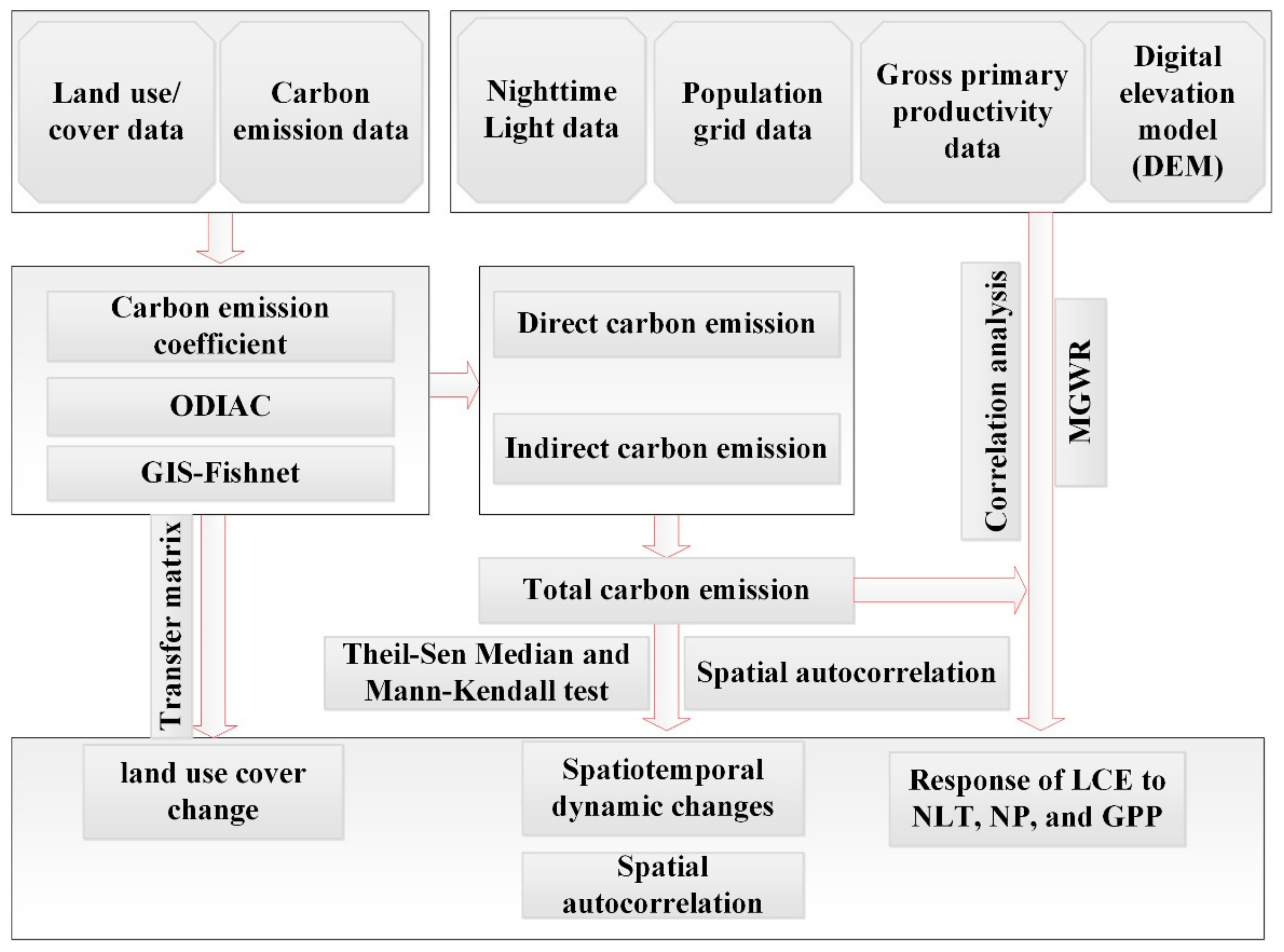
In order to investigate the response mechanism of LCEs to human and natural factors in the GZA, we used the carbon emission coefficient method and the Open-source Data Inventory for Anthropogenic CO2 (ODIAC) data to calculate the annual direct land carbon emissions (DLCE) and indirect land carbon emissions (ILCE) from 2000 to 2019, respectively. We also used the Fishnet tool in ArcGIS 10.8 to calculate the total LCEs in the GZA by overlying the DLCE map and ILCE map. Then, trend analysis and spatial autocorrelation analysis were used to study the spatiotemporal changes in LCEs, and correlation analysis and MGWR models were adopted to analyze the driving forces of LCEs. The overall technical roadmap of this study is illustrated in Figure 2.

2.3. Data Sources and Processing

In this study, the land use/cover data, carbon emission data, nighttime light (NLT) data, population grid data, and gross primary productivity (GPP) data were used to analyze the spatio-temporal dynamics of land use carbon emissions and their driving factors in the study area (Table 1). The specific data information is as follows:
(1) Land use/cover data: the annual land use/cover data from 2000 to 2019 at a spatial resolution of 300 m were collected from the European Space Agency (http://maps.elie.ucl.ac.be/CCI/viewer/, accessed on 1 June 2022) and were divided into seven types, including cropland, grassland, forestland, wetland, water, unused land, and construction land (Figure 1c and Figure A1).
(2) Carbon emission data: the monthly carbon emission datasets from 2000 to 2019 were published by the Open-source Data Inventory for Anthropogenic CO2 (ODIAC) (http://db.cger.nies.go.jp/dataset/ODIAC/data_policy.html, accessed on 1 May 2022). These datasets had a spatial resolution of 1 km and were estimated by combining the space-based nighttime light data and the individual power plant emission, a method that has been widely used for a variety of research applications (e.g., CO2 flux inversion, urban emission estimation, and observing system design experiments) [9].
(3) Nighttime Light (NLT) data: the Defense Meteoro-logical Satellite Program Operational Line scan System (DMSP-OLS) and Visible Infrared Imaging Radiometer Suite Day/Night Band (VIIRS/DNB) Nighttime Light (NLT) data were obtained from the NOAA website’s NGDC data center (https://www.ngdc.noaa.gov/eog/download.html, accessed on 4 August 2022) [31].
(4) Population grid data: the population grid datasets at a spatial resolution of 1 km for the years 2000–2019 were obtained from World Pop (https://www.worldpop.org/project/list, accessed on 13 August 2022).
(5) Gross primary productivity (GPP) data: the annual GPP datasets at a spatial resolution of 1 km were derived from the National Tibetan Plateau/Third Pole Environment Data Center (https://data.tpdc.ac.cn/zh-hans/data/582663f5-3be7-4f26-bc45-b56a3c4fc3b7, accessed on 13 September 2022).
In order to keep the resolution of all data consistent, we resampled these data to ensure that the data resolution was 1 km.

2.4. Calculation of LCE

In this study, the LCE consist of DLCE and ILCE [14]. Specifically, the DLCE represent direct carbon emissions from grassland, forestland, cropland, water, and unused land, while ILCE represent carbon emissions from construction land and cropland through energy consumption. In this study, the carbon emission coefficient method was used to simulate the DLCE of different land types in the GZA [32]. According to the previous studies and IPCC [16], we determined the carbon emission coefficients for different land use types in the study area, as shown in Table 2. Meanwhile, the DLCE can be calculated according to Equation (1). In addition, we derived the monthly emission data regarding the production of fossil-fuel CO2 emissions at a spatial resolution of 1 km from the ODIAC platform. Then, the annual ILCE can be calculated from the monthly data based on Equation (2) (Figure A2).
D L C E = C i = S i × V i
I L C E = M i
where Ci represents the DLCE for the land-use types i (t); Si donates the area of the land-use type i (hm2); and Vi means the carbon emission coefficient of the land-use type i (t⋅hm−2⋅a−1). Mi donates the monthly carbon emissions data obtained from the ODIAC (t) [9].

2.5. Theil-Sen Median Trend Analysis and Mann–Kendall Test

The Theil-Sen Median was used to analyze the spatial dynamics trend of LCE from 2000 to 2019 in the GZA, while the significance of the change was determined by the Mann–Kendall test [33].
S β = M e d i a n L C E j L C E i j i , 2000 i < j 2019
where S indicates the trend of LCE; LCEj is the LCE value in year j, and LCEi is the LCE value in year i. When S > 0, LCE showed an increasing trend. Conversely, when S < 0, LCE indicated a decreasing trend.
The Mann–Kendall test can be expressed as follows [34]:
I = i = 1 n 1 j = i + 1 n sgn L C E j L C E i , 2000 i < j 2019
sgn L C E j L C E i = 1 , L C E j L C E i > 0 0 , L C E j L C E i = 0 1 , L C E j L C E i < 0 , 2000 i < j 2019
Z = I 1 V a r I , I > 0 0 ,     I = 0 I + 1 V a r I , I < 0
V a r I = n n 1 2 n + 5 18
where I represents the test statistic; Z indicates the standardized test statistic at a certain significance level α, when |z| > z_(1 − α/2) represents a significant change in the time series at the α level. The variation trend of the LCE in this study can be divided into the 5 change types based on the 95% significance test (Table 3) [9].

2.6. Spatial Auto-Correlation Analysis

In this study, we used the Global Moran’s I index to detect the spatial auto-correlation of LCE to analyze the degree of aggregation or dispersion of the spatial features in the GZA. The calculation method of Global Moran’s I can be expressed as follows [17]:
Moran s   I = n i = 1 n j = 1 n w i j ( Z i Z ¯ ) ( Z j ¯ Z ¯ ) i = 1 n j = 1 n w i j i = 1 n ( Z j Z ¯ ) 2
where n is the number of spatial units, Zi and Zj represent the carbon emissions of spatial units i and j (1 ≤ i ≤ 23,972; 1 ≤ j ≤ 23,972), and Wij is the spatial weight matrix of the adjacent prefecture-level units i and j.
Additionally, the Local Moran’s I index was used to detect the local spatial auto-correlation, which can be expressed as follows:
Local   Moran s   I = n ( x i x ¯ ) j = 1 n w i j x j x ¯ i = 1 n ( x i x ¯ ) 2
where n denotes the number of space units; xi and xj represent the carbon emissions of space units i and j; and Wij is the weight. When I > 0, it indicates that there is a positive spatial auto-correlation between adjacent regions, showing a ‘high-high (H-H)’ or ‘low-low (L-L)’ type, indicating that there is a high (low) concentration of carbon emissions between adjacent regions. When I < 0, it indicates that there is a negative spatial auto-correlation between adjacent regions, which is ‘high-low (H-L)’ or ‘low-high (L-H)’ type, indicating that high (low) carbon emission regions are surrounded by low (high) carbon emission regions [35].

2.7. Analysis of the Driving Factors Affecting Carbon Emissions

Previous studies have pointed out that the LCE are mainly influenced by both human and natural factors [10]. Considering the analysis of LCEs drivers on a grid scale and the availability of grid-scale data, we selected the NTL, PD, and GPP to evaluate the impacts of human and natural factors on LCE levels in the study area. For the three driving factors, the NLT can reflect the intensity of regional economic development and urbanization development level, and the changes in PD will directly cause changes in carbon emissions. Moreover, the GPP can reflect the carbon sink level of vegetation.

2.7.1. Correlation Analysis

In this study, correlation analysis was used to investigate the relationship between the different driving factors and LCE from a global dimension, which can be expressed as follows [15]:
R x y = i = 1 n ( x i x ¯ ) ( y i y ¯ ) i = 1 n ( x i x ¯ ) 2 i = 1 n ( y i y ¯ ) 2
where n is the total year; xi and yi represent the value of the driving factor and the LCE of the i-th year; and x ¯ and y ¯ represent the average value from 2000 to 2019.

2.7.2. The Multi-Scale Geographically Weighted Regression (MGWR) Model

In terms of driving factors that affect carbon emissions, many scholars have adopted the geographical weighted regression (GWR) model for analysis. However, the GWR model uses the ‘best average’ bandwidth, which leads to the same spatial scale characteristics of all explanatory variables, and consequently, cannot reflect the spatial differences. Therefore, the multi-scale geographic weighted regression (MGWR) model is used in this study to analyze the influence strength of different driving factors on LCE [15]. The specific calculation method is as follows:
y i = β 0 u i , v i + k = 1 p β b w k u i , v i x i k + ε i
where (ui, vi) denotes the spatial coordinate of the i-th geographical location; bwk is the bandwidth of the regression coefficient of the k-th explanatory variable; and β0(ui, vi) is the intercept term of the model at i.

3. Results

3.1. The Land Use Cover Change in the GZA

This study reclassified the remote sensing data of land use data in the GZA from 2000 to 2019 based on the ArcGIS 10.8, and then carried out land use transfer matrix analysis. As shown in Figure 3, the proportion of cropland converted to construction land between 2000 and 2019 was relatively large (Figure 3b), which was mainly observed in most areas of Xi’an City, the central area of Baoji City, and the southern area of Xianyang City, accounting for 76.36% of the total area (Figure 3a). Meanwhile, 3.49% of the areas have changed from grassland to construction land, which mainly occurred in the surrounding area of Baoji and Xi’an City. The proportion of wetland, forest, and unused land converted to urban land was relatively small. In addition, 7.21% of the regions have been transformed from forest to grassland, mainly distributed in most areas of Baoji City. These transformations showed that the urbanization process was fast in this period, and a large number of cultivated land was occupied to develop cities. Table 4 showed that the cropland increased by 79.47 km2 from 2000 to 2019, mainly due to the conversion of grassland (48.96 km2) and forest (30.51 km2) to cropland. The total increase in forestland was 190.17 km2, mainly due to the conversion of grassland (105.57 km2) and cropland (84.6 km2) to forestland. The increase in grassland was mainly attributed to the transformation from forestland (209.52 km2). In addition, the largest increase occurred in construction land. Among these land-use changes, the area converted from cropland to construction land was the largest (2218.05 km2), followed by the grassland (101.43 km2).

3.2. Spatiotemporal Changes of LCE

As shown in Figure 4, the LCE in the study area showed a significantly increasing trend from 2000 to 2019 (1.76 million t; p < 0.01). Specifically, the average value of LCE in this period was 31.30 million t; the total amount of LCE in 2000 was 13.58 million t; LCE increased to 31.02 million t in 2009; and the total amount of LCE reached 43.66 million t in 2019. From 2000 to 2009, the growth rate of LCE was relatively fast, but the growth rate showed a significant downward trend from 2010 to 2019. This change may serve as a great sign in terms of China’s emission reduction goals and the tasks established at the 2009 Copenhagen Conference and the 2015 Paris Climate Conference.
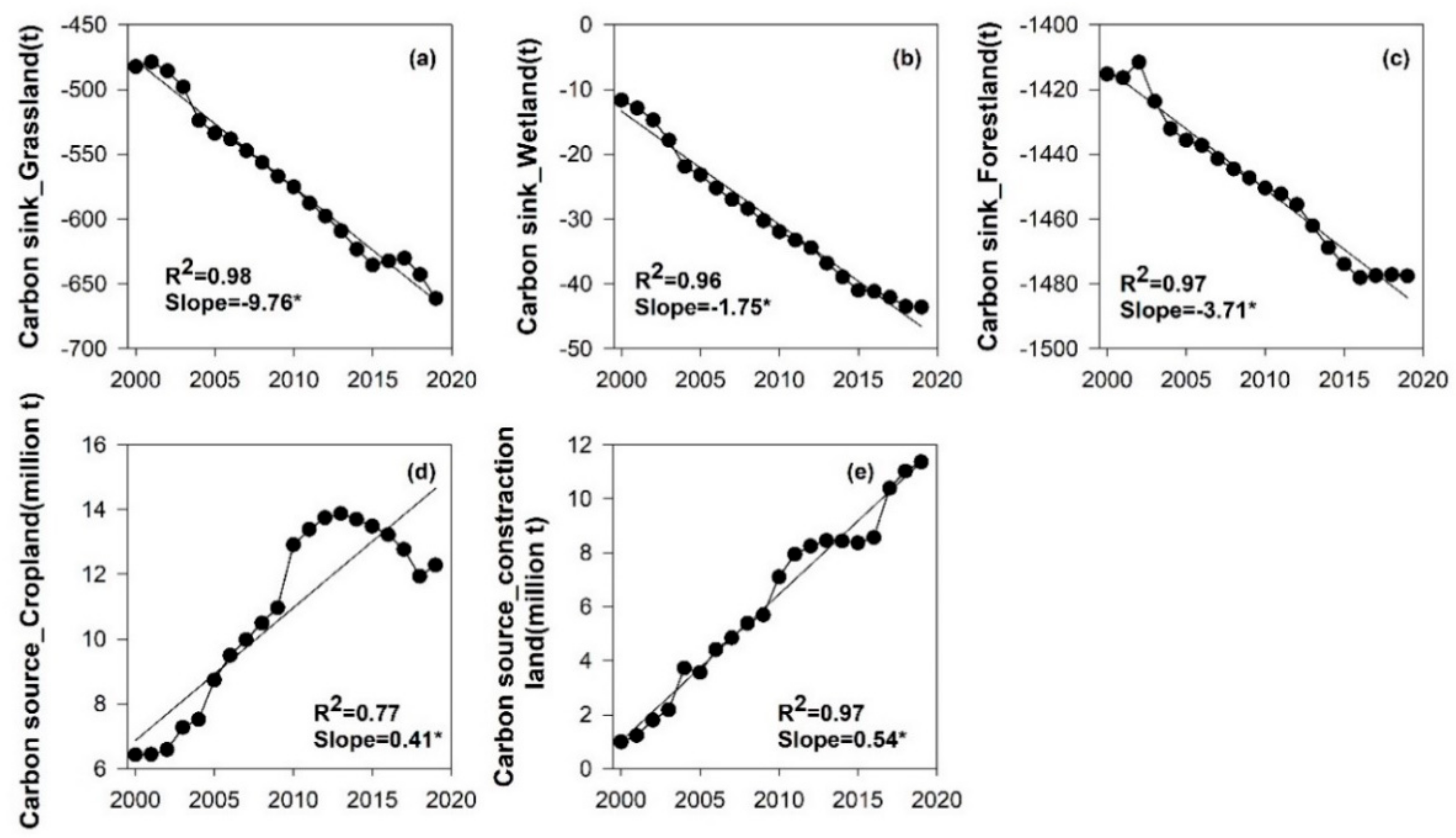
In addition, we found that grassland, forestland, and wetland all showed negative carbon emissions (Figure 5), indicating that these land types had an important carbon absorption role, therefore showing carbon sink. In general, the carbon absorption of these three land use types showed a significant downward trend from 2000 to 2019. By contrast, cropland and construction land were mainly characterized by positive carbon emissions. In terms of inter-annual changes, carbon emissions from cropland showed an obvious increase trend from 2000 to 2013 and then indicated a downward trend, which may be related to the conversion of large amounts of cropland area to construction land. Meanwhile, the carbon emissions in the construction land showed a significant increase trend (0.54 million t/a; p < 0.01). These indicate that the increase of carbon emissions in the GZA in the past two decades has mainly been due to the increasing energy consumption and human-related carbon emissions encouraged in the process of urbanization.
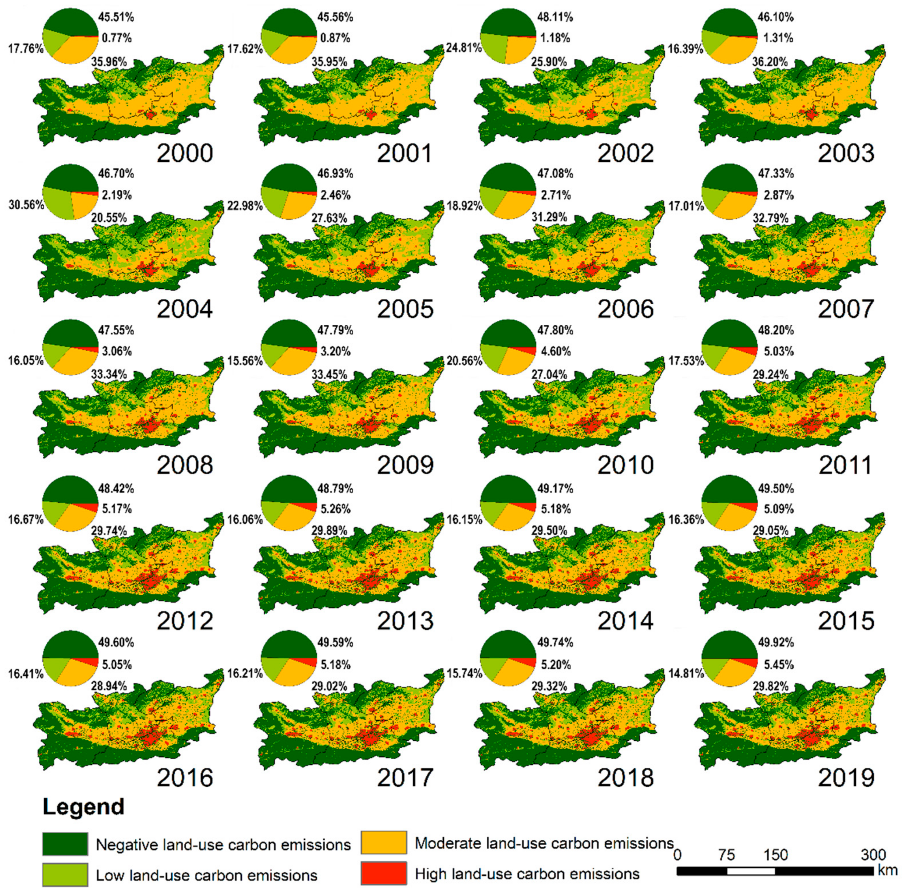
Based on the natural break point method, the land-use carbon emissions from 2000 to 2019 were divided into four types: high land-use carbon emissions, moderate land-use carbon emissions, low land-use carbon emissions, and negative land-use carbon emissions (Figure 6), and then the change characteristics of different types of land carbon emissions were analyzed. Specifically, the regions with high land-use carbon emission levels accounted for about 3–5% of the total area, showing an upward trend (from 0.77% in 2000 to 5.45% in 2019). These areas were mainly distributed in the Xi’an and Xianyang urban areas, which may have been caused by the acceleration of urbanization and the intensification of energy consumption. The regions with moderate land-use carbon emission grade occupied nearly 33% of the total area, indicating a decreasing trend overall (from 35.96% in 2000 to 29.82% in 2019). These areas were mainly observed in the cropland distribution areas of Guanzhong, indicating that the improvement of agricultural farming methods has promoted the reduction of carbon emissions in recent years. The regions with low land-use carbon emission grade accounted for about 16% of the total coverage area and also showed a downward trend (from 17.76% in 2000 to 14.81% in 2019). By contrast, the coverage area of negative land-use carbon emission rating occupied nearly 48% of the total area, and showed a slight increase (from 45.51% in 2000 to 49.92% in 2019). These areas were mostly concentrated in the southern and northern parts of GZA, where grassland and forestland were widely distributed, implying that ecological restoration has significantly promoted the regional carbon sink in recent years.
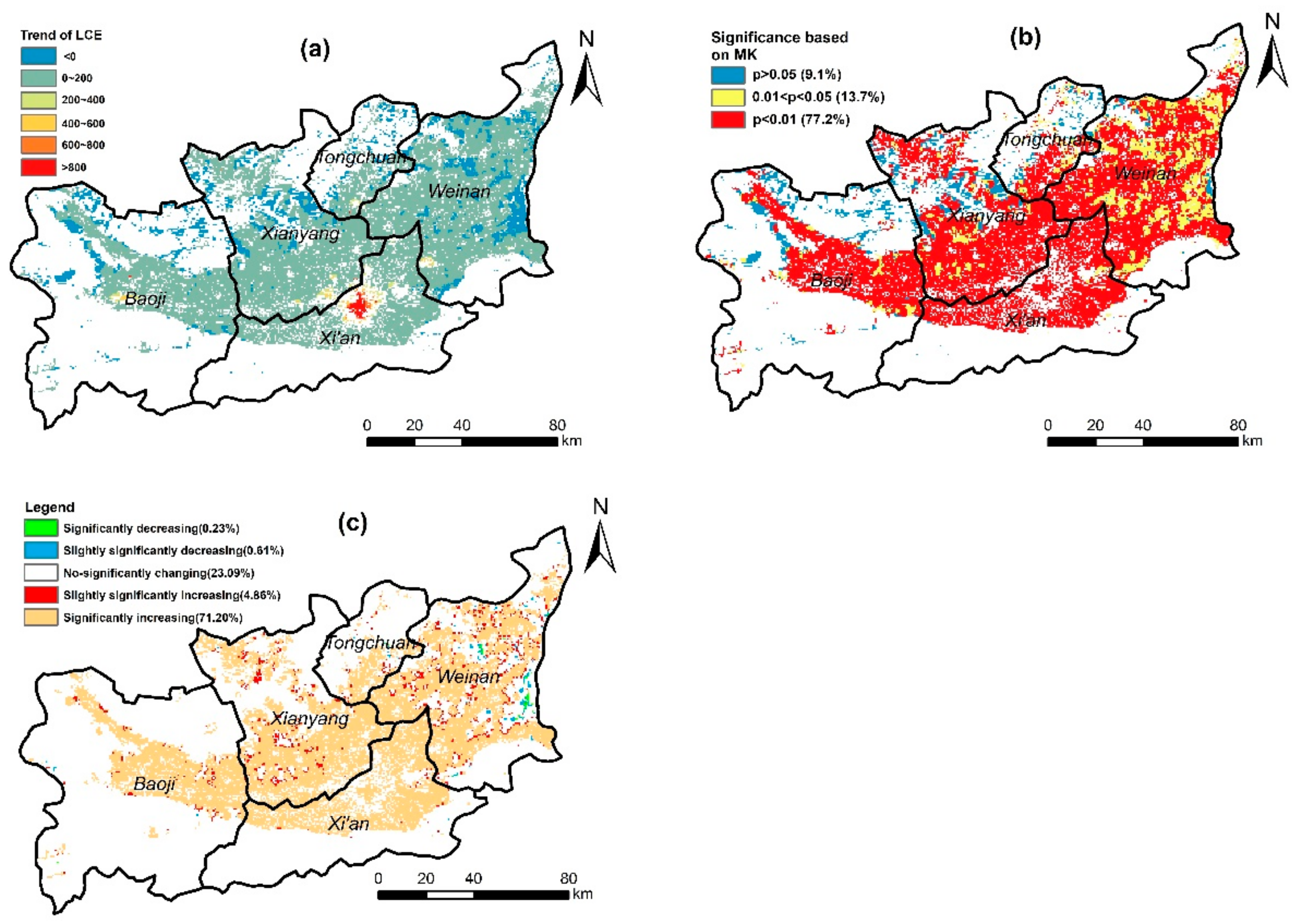
The spatial change trend and significance test of the LCE from 2000 to 2019 in GZA is shown in Figure 7. As shown in Figure 7a, the regions with a decreasing trend in LCE were mainly distributed in the eastern parts of Weinan and the central parts of Xianyang, while cities such as Xi’an showed an obvious increase in LCE. The increase rate of LCE was relatively low in other regions. The MK test results indicated that 77.2% of the total area had significant changes in LCE in the study area (Figure 7b). However, areas with slightly significant changes in LCE were mainly scattered in Weinan and other areas, accounting for 13.7% of the total area. Meanwhile, the regions with insignificant changes in LCE only accounted for 9.1% of the total area. Through the superposition analysis of the LCE change rate and the significance test (Figure 7c), the regions where the LCE showed an increasing trend accounted for 76.06% of the total area. Specifically, regions with a significant increase in LCE occupied 71.20% of the total area; they were mainly distributed in the central and eastern parts of GZA, such as the northern part of Xi’an City, the southern part of Xianyang City, and most parts of Weinan City. These areas were mainly dominated by cropland vegetation. The regions with a slightly significant increase in LCE were mainly scattered in Xianyang and Weinan City, accounting for 4.86% of the total area. In contrast, the regions with significant and slightly significant decreases in LCE accounted for 0.84% of the total area; they were mainly distributed in the eastern part of Weinan City. The remaining 23.09% of regional LCE showed no significant change, with these areas mainly concentrated in the forest area in the south of the Guanzhong region.

3.3. Spatial Autocorrelation of LCE

Table 5 shows that the Global Moran’s I was higher than 0 for different years within the 2000–2019 range, with the normal statistic Z values found to be higher than 2.58 and the p values found to be significant at the 5% level (i.e., p < 0.05), indicating that LCE showed a significant positive spatial correlation in the GZA. In addition, temporally, Moran’s I of LCE experienced an overall increasing trend in GZA from 2000 to 2017 (from 0.1117 in 2000 to 0.1755 in 2017), but it began to decrease after 2017, indicating that the spatial correlation of LCE in the GZA was increasing and more spatially concentrated, but there was somewhat of a decrease over time after 2017.
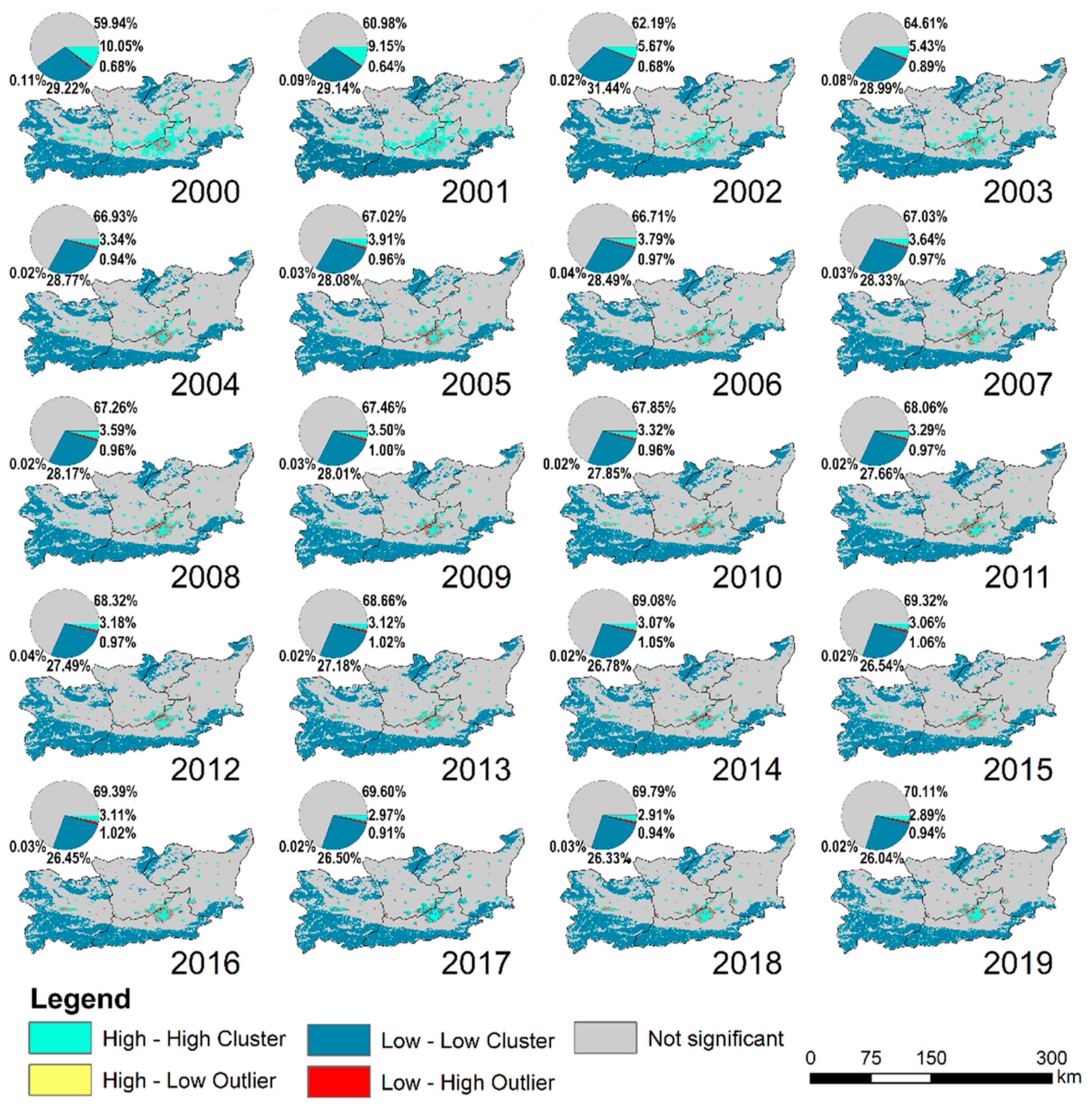
The local spatial autocorrelation clustering results of LCE from 2000 to 2019 were as follows (Figure 8). From 2000 to 2001, the H-H agglomeration area of LCE in the whole study area was distributed in the central urban agglomeration of the study area, including Xi’an, Xianyang and, Baoji. These regions had dense cities and large populations, which led to high energy consumption, resulting in high concentrations of carbon emissions. At this time, the H-H agglomeration area is large (accounting for about 10%). However, from 2002 to 2019, the H-H agglomeration area showed an obvious downward trend, from 5.67% in 2002 to 2.89% in 2019. During the period of 2012–2019, the H-H agglomeration area mainly formed core urban areas with rapid economic development and population growth, such as Xi’an and Baoji. The L-L agglomeration area was always distributed in scale, and the spatial distribution range was relatively stable (26~29%), mainly distributed in the southwest parts of the GZA, such as the western and southern areas of Baoji City, the southern areas of Xi’an City, and Weinan City; the area was also distributed in the junction area of Tongchuan and Xianyang. These areas were mainly located on the east side of the Qinghai-Tibet Plateau and the southwest side of the Loess Plateau, and most of them were located on the edge of the Qinling Mountains, with high vegetation coverage, strong ecological environmental constraints, sparse population, inadequate development of the central city itself, and a weak connection with the surrounding cities, resulting in low carbon emissions. The H-L aggregation area was the smallest part of the study area. From 2000 to 2004, the L-H aggregation area showed an increase and remained stable after 2004, accounting for about 1%.

3.4. The Response of LCE Changes to Different Driving Factors

3.4.1. Analysis of the Driving Factors Affecting LCE Changes at the Global Dimension

As shown in Figure 9, the average correlation coefficients between LCE and driving factors (NTL, PD, and GPP) in the study area from 2000 to 2019 were 0.13, 0.21, and −0.05, respectively. Specifically, the area of positive correlation between LCE and NTL in the GZA was about three times that of negative correlation, accounting for 77.39% and 22.61% of the total area, respectively. The area with a significant positive correlation (0~0.5) accounted for 38.84% of the total area. The negative correlation area (−0.5~−1) only accounted for 5.31%, which was mainly observed to be distributed in Xi’an and Xianyang. The proportions of positive and negative correlations between LCE and PD were relatively close. The positive correlation area (0~0.5) accounted for 30.68% of the total area, which was mainly found in the urban area of Xi’an, while other areas were scattered in a dotted pattern. The negative correlation area (0~−0.5) occupied 29.19% of the total area, which was mainly distributed in the eastern part of Baoji, the western part of Weinan, and the southern part of Xianyang. The area of positive correlation between LCE and GPP in the study area was slightly smaller than that of negative correlation, accounting for 66.44% and 33.56% of the total area, respectively. In general, the area of positive and negative correlation was more concentrated. The area with a positive correlation (0~0.5) accounted for 51.59% of the total area, mainly distributed in the northwest of Baoji, the middle of Weinan, and the central and western regions. The area with a negative correlation (0~−0.5) occupied 30.29%, mainly distributed at the junction of southern Xianyang and northern Xi’an, the central and eastern part of Baoji, and the eastern part of Weinan. The analysis showed that the correlation between LCE and the above three factors in the study area has obvious spatial heterogeneity, which may be related to the different responses of LCE to the change of factors.

3.4.2. Analysis of the Driving Factors Affecting LCE Changes at the Local Dimension

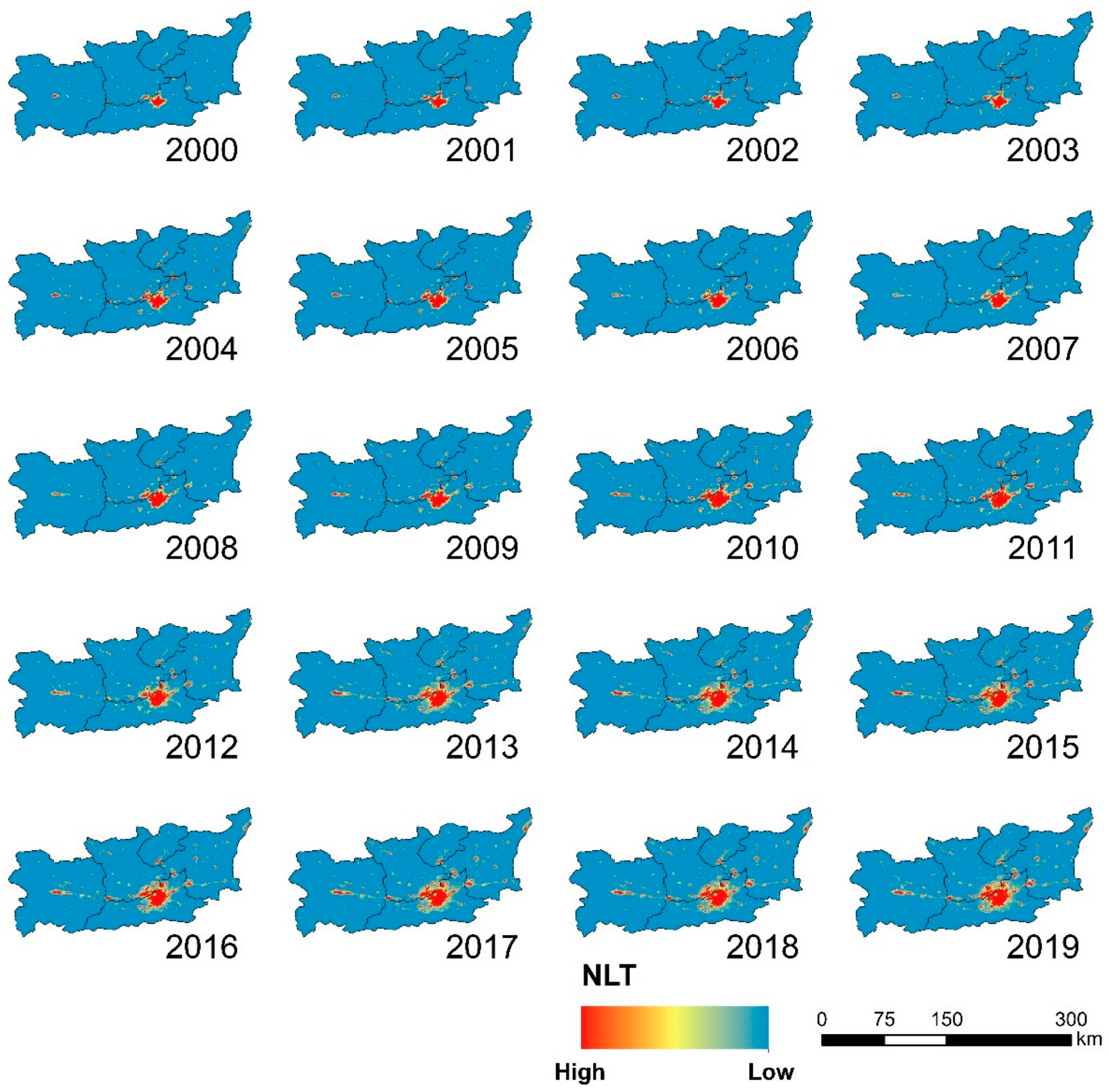
For NTL variables, the estimated coefficients of most regions in the GZA were significantly positive (Figure 10a,d), implying that the LCE was increasing with the increase of the NTL index. Given that the NTL index can explain the level of urbanization and energy consumption to a certain extent, the acceleration of urbanization significantly promotes the increase of LCE. It showed that the high-value areas of the NTL index from 2000 to 2019 were mainly concentrated in the Guanzhong urban agglomeration area. It can be seen that the urban agglomeration area, with Xi’an as the center, was driving the development of the surrounding areas (Figure A3). From 2000 to 2019, the land-use type in the high-value area of the coefficient estimation was mainly constructed land and cropland, while the land-use type in the low-value area of the coefficient estimation was mainly forest. The NTL index and LCE are mainly positively correlated. Therefore, the higher NTL index indicated that the land-use type was to be a carbon source. On the other hand, compared with 2000, the estimated average of the minimum and maximum levels of coefficients increased in 2019.
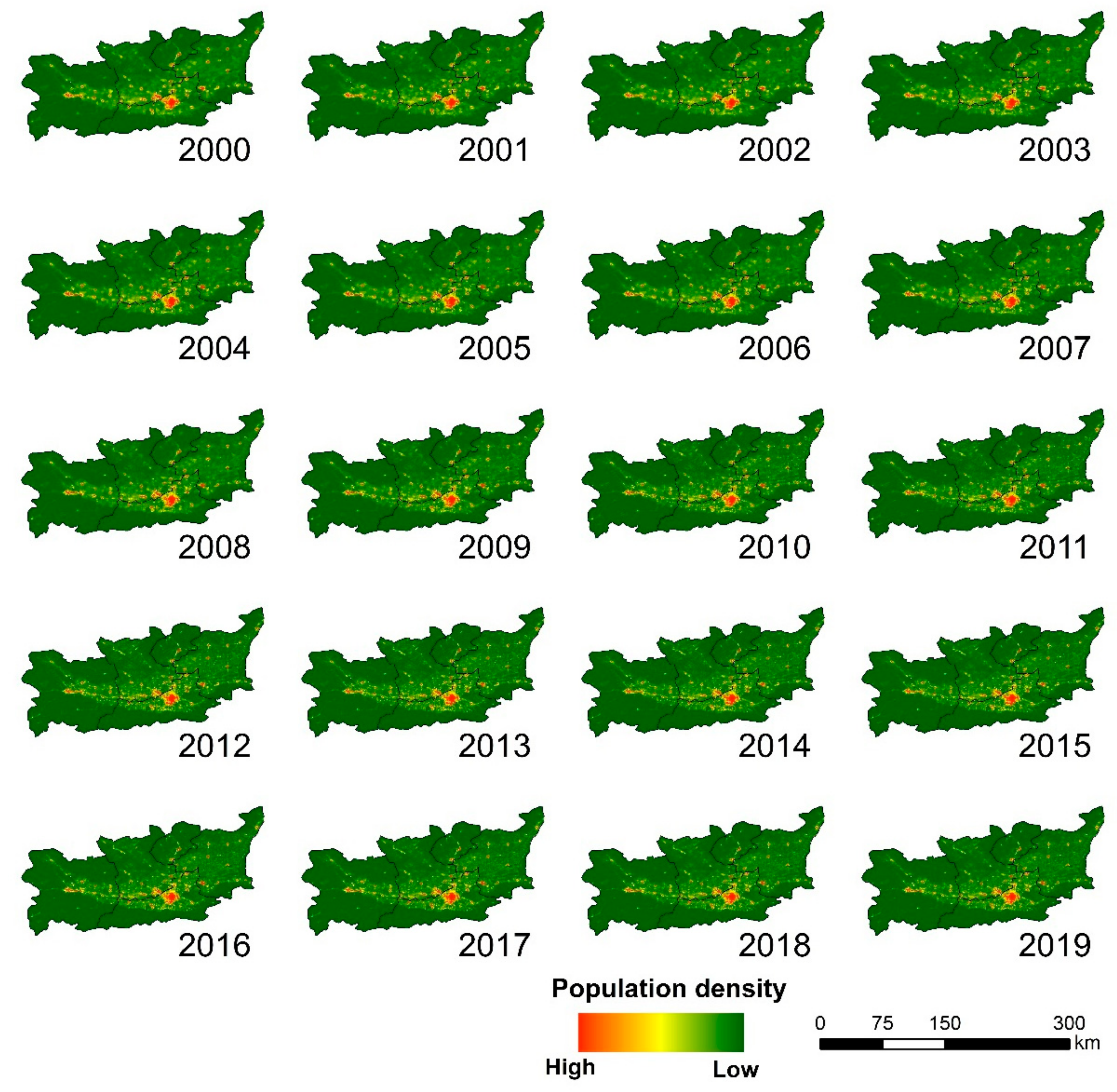
For the PD variables, the coefficient estimation indicated a significant spatial pattern of polarization across the whole study area (Figure 10b,e). Similar to the NLT, the high-value areas of PD were also distributed in urban agglomeration areas, such as Xi’an, Xianyang, and Baoji, and the high-value areas of PD showed an increasing trend from 2000 to 2019 (Figure A4). The significant negative correlation effect was mainly observed in grassland, cropland, and the forest area in the west of Xianyang, while the significant positive correlation effect was mainly found in construction land and cropland area. In 2000, the high estimated value was relatively small, mainly distributed in the north of Xianyang. Compared with 2000, there were concentrated areas with a high estimated value in all cities in 2019, which indicated that the development of the five cities had a center of gravity, and the low-value areas were distributed in the west and east of the study area.
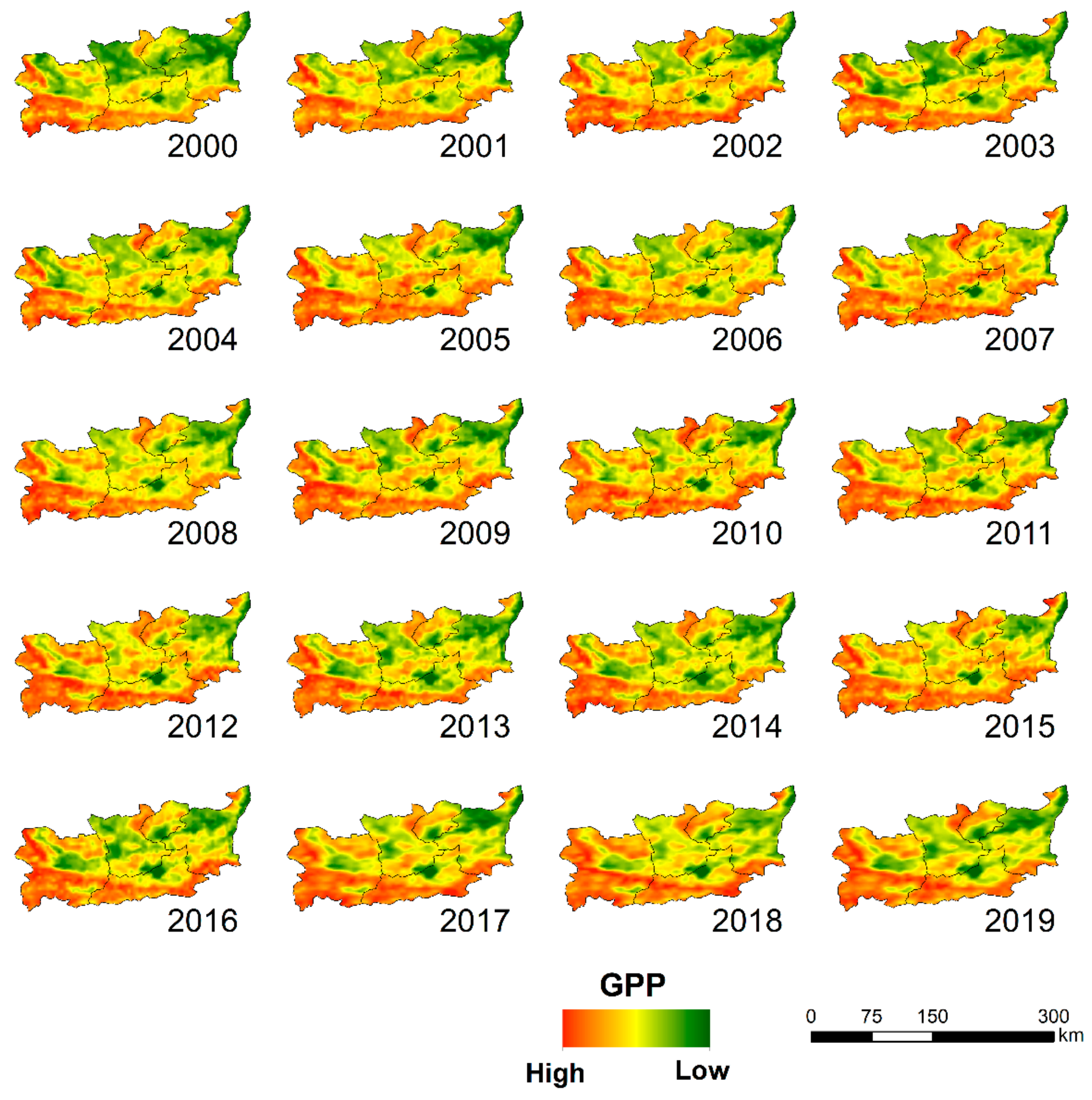
For GPP variables, the regression coefficients of most areas in the GZA showed significant negative values (Figure 10c,f), indicating that LCE tended to decrease with the increase of GPP. From 2000 to 2019, the total GPP in the study area indicated an increasing trend (Figure A5). The frequency of human activities in low-value areas was high, resulting in damage to the vegetation environment or growth difficulties. High-value areas were mainly distributed in the Qinling Mountains in the south of GZA, where the vegetation coverage was high and the ecological environment was well-preserved. Based on the spatial distribution results estimated by the correlation coefficient between GPP and LCE in 2000 and 2019, the high-value areas were mainly distributed in the southern part of Xianyang and the eastern part of Weinan. The low-value areas were mainly distributed in the junction of Xi’an, Xianyang, and Weinan, and in the middle and eastern parts of Baoji. From 2000 to 2019, the land-use types in the areas with high coefficient estimates were forest and grassland, while the land-use types in the areas with low coefficient estimates were construction land and cropland. In general, GPP and LCE showed a negative correlation, mainly because the land-use types in areas with high GPP value tend to be carbon sinks. On the other hand, compared with 2000, the estimated value of the coefficient generally declined in 2019.

4. Discussion

Scientific estimation and dynamic monitoring of the variation trend of LCEs in a long time series is the scientific basis and basic guarantee for formulating, implementing, and evaluating regional carbon emission reduction strategies [12]. Many previous studies have used different methods to estimate regional LCEs, such as using energy statistical yearbooks to calculate carbon emissions [12], but this method cannot achieve grid-scale carbon emissions estimation [36]. Meanwhile, carbon emission research based on traditional statistical data is often limited to national or provincial levels due to data limitations, and it is difficult to refine to spatial scales which could provide more powerful support for formulating regional and differentiated carbon emission reduction policies [37]. In addition, some studies selected the BK model to estimate LCEs. Although this model can quantify the impact of land-use change on carbon emissions, it is difficult to obtain parameters [38]. Compared to previous studies, this study used the carbon emission coefficient method to calculate direct LCEs and introduced the carbon emission grid data of fossil fuel data released by the ODIAC platform to calculate indirect LCEs [39]. Through the superposition of direct and indirect carbon emission results, we analyzed the temporal and spatial changes of LCEs in the GZA at a grid scale. The method used in this study mainly calculated indirect carbon emissions using 1 km high-resolution grid data; this simple process is highly accurate [40].
This study found a significant increase in LCEs in the GZA (Figure 4), which was consistent with most previous research [18,31,32,35]. Especially for urban and cultivated areas, the LCEs show a significant increase (Figure 4). The land use transfer matrix shows (Figure 3) that the area of construction land in the GZA significantly increased since 2000, indicating that the urbanization process accelerated during this period. In the process of urbanization, the increase in population density and various anthropogenic energy consumptions has become the dominant factor that increases LCEs [41]. Spatially, regions with high LCEs were mainly distributed in the Xi’an, Xianyang, and Baoji urban agglomerations (Figure 6), and this distribution pattern was closely related to the development of heavy industry and the human energy consumption in these cities [42]. For cropland, this study found that LCE showed a significant increase in large areas of cropland. Although cropland had a certain carbon sequestration effect, it became a major carbon source due to the increased use of agricultural films, pesticides, and diesel fuel in various agricultural production activities [9]. For grassland and forest areas, this study found that the LCEs showed negative values, indicating that these areas showed obvious carbon sinks (Figure 5). However, due to the overall small changes in the areas of grassland and forest, the impact of grassland and forest changes on the total amount of carbon emissions was relatively weak (Figure 3). Considering the analysis of LCEs drivers on a grid scale, this study selected NLT, PD, and GPP as the driving factors to explore the impact of urbanization, population, and ecological restoration on LCEs. The NLT can reflect the intensity of regional economic development, and changes in PD will directly cause changes in carbon emissions [43]. The GPP can reflect the carbon sink level of vegetation [44]. This study found that NLT, PD, and GPP have significant spatial heterogeneity in their impact on LCE in the study area (Figure 9). The NLT, PD, and LCE showed a positive correlation, while GPP showed a negative correlation with LCE (Figure 10). The results of this study indicated that energy consumption driven by regional industrial agglomeration, urban scale expansion, and population aggregation to cities became the main reason for the increase in LCEs in the study area. This was consistent with most previous results [1,35]. Based on the above analysis, the GZA should prioritize coordinated development, overall planning, the formulation of carbon emission reduction policies and carbon trading volumes, and the implementation of systematic and differentiated emission reduction policies to strive to reach the carbon peak as soon as possible [11,45]. From the perspective of the spatial distribution and agglomeration status of carbon emissions, cities will still be the basic implementation unit for future carbon emission reduction [46]. Therefore, it is necessary to actively improve energy utilization efficiency and optimize industrial and energy structures [47]. Economic growth and urbanization construction were still the main reasons for the growth of LCEs in the study area. Therefore, in the implementation of carbon emission reduction policies, it is necessary to achieve regional low-carbon and green development while maintaining stable economic growth. In addition, in combination with the regional resource and environmental carrying capacity and territorial spatial planning, we should reasonably control population size and urban development efforts, and optimize urban spatial development structures and industrial layouts [11,48].
In this study, the carbon emission grid data of the ODIAC platform was superimposed with the direct carbon emission results calculated by the carbon emission coefficient method, and then the LCE in GZA was calculated from 2000 to 2019. Based on the Moran’s I, correlation coefficient and MGWR model, the spatiotemporal change characteristics and driving factors of carbon emissions were evaluated. The research results have an important reference value for the evaluation and driving mechanism analysis of LCE in Shaanxi Province [18]. However, in the process of measuring LCE, the carbon emission coefficient of land-use types was based on the existing research, which was somewhat different from the research area. Therefore, it is necessary to further improve the data regarding the research area, comprehensively consider carbon sources and sinks, and improve the accuracy of carbon emission calculations in the future [49]. In addition, due to the many driving factors of carbon emissions, only the nighttime light index, population density, and GPP were selected in this study. Therefore, more possible influencing factors should be considered when analyzing the influencing factors of land use carbon emissions in the future.

5. Conclusions

This study analyzed the spatial and temporal changes of LCE based on carbon emission data and land-use data, and examined the effects of NTL, PD, and GPP on LCE. During the period of 2000–2019, the average value of LCE was 31.30 million t. Temporally, the total amount of LCE showed a significant increase from 2000 to 2019 (1.76 million t; p < 0.01). Meanwhile, the carbon absorption of grassland, forestland, and wetland showed a significant downward trend, while the carbon emissions in the construction land showed a significant increase (0.54 million t/a; p < 0.01). Spatially, regions where the LCE significantly increased occupied 71.20% of the total area, which was distributed in the central and eastern parts of the study area. Global Moran’s I of LCE indicated that the LCE showed a significant positive spatial correlation, and had a remarkable aggregation state. The local spatial auto-correlation clustering results of the LCE were mainly represented by the H-H and L-L agglomerations. The H-H agglomeration area of LCE was distributed in the central urban agglomeration of the study area, and showed a downward trend from 2002 to 2019. The L-L agglomeration area was always distributed in the southwest part of the GZA with low carbon emissions. The correlation analysis showed that the average correlation coefficients between LCE and NTL, PD, and GPP were 0.13, 0.21, and −0.05, respectively, which showed a large spatial heterogeneity distribution characteristic. The MGWR analysis also indicated that the NLT and PD had obvious positive effects on LCE, especially for urban agglomeration areas, such as Xi’an and Baoji, while GPP has obvious negative effects on carbon emissions in most areas, mainly due to the carbon sink effect of ecosystems, such as forests and grasslands. The results of this study have an important reference value for the formulation of carbon emission reduction policies and the development of a low-carbon social economy in the GZA and even the whole Shaanxi province.

Author Contributions

Conceptualization, Y.L., Z.L. and P.H.; methodology, Z.W. (Zijun Wang) and Y.Y.; software, Z.W. (Zijun Wang) and Y.Y.; formal analysis, Z.W. (Zijun Wang), Y.Y., W.Z. and Z.Z.; data curation, Y.Z.; writing—original draft preparation, Z.L. and S.J.; writing—review and editing, Z.L. and S.J.; visualization, Y.W. and Y.L.; supervision, B.F.; project administration, Z.W. (Zhongming Wen) and W.Y.; funding acquisition, Z.W. (Zhongming Wen) and W.Y. All authors have read and agreed to the published version of the manuscript.

Funding

This research was funded by Shaanxi agricultural rural economic and technological system construction project, grant number NYKJ-2020-YL-18, Startup fund for doctoral research of Northwest A&F University, grant number 2452020186, and Special project of science and technology innovation plan of Shaanxi Academy of Forestry Sciences, grant number SXLK2022-02-7.

Institutional Review Board Statement

Not applicable.

Informed Consent Statement

Not applicable.

Data Availability Statement

The data presented in this study are available on request from the corresponding author.

Acknowledgments

The authors would like to thank all the data providers, including Loess plateau science data center, National Earth System Science Data Sharing Infrastructure, National Science & Technology Infrastructure of China (http://loess.geodata.cn), ODIAC Fossil Fuel Emission Dataset (http://db.cger.nies.go.jp/dataset/ODIAC/data_policy.html), European Space Agency (http://maps.elie.ucl.ac.be/CCI/viewer/) and National Tibetan Plateau/Third Pole Environment Data Center (https://data.tpdc.ac.cn/zh-hans/data/582663f5-3be7-4f26-bc45-b56a3c4fc3b7).

Conflicts of Interest

The authors declare no conflict of interest.

Appendix A

Figure A1. Land-use types of the study area from 2000 to 2019.
Sustainability 15 07730 g0a1
Figure A2. The spatial patterns of the carbon emission data obtained from the ODIAC between 2000 and 2019.
Sustainability 15 07730 g0a2
Figure A3. Spatial patterns of nighttime light from 2000 to 2019.
Sustainability 15 07730 g0a3
Figure A4. Spatial patterns of population density from 2000 to 2019.
Sustainability 15 07730 g0a4
Figure A5. Spatial patterns of GPP from 2000 to 2019.
Sustainability 15 07730 g0a5

References

  1. Liu, J.; Peng, K.; Zuo, C.; Li, Q. Spatiotemporal variation of land-use carbon emissions and its implications for low carbon and ecological civilization strategies: Evidence from Xiamen-Zhangzhou-Quanzhou metropolitan circle, China. Sustain. Cities Soc. 2022, 86, 104083. [Google Scholar] [CrossRef]
  2. Huang, Z.; Li, S.; Gao, F.; Wang, F.; Lin, J.; Tan, Z. Evaluating the performance of LBSM data to estimate the gross domestic product of China at multiple scales: A comparison with NPP-VIIRS nighttime light data. J. Clean. Prod. 2021, 328, 129558. [Google Scholar] [CrossRef]
  3. Lin, B.; Zhou, Y. How do economic growth targets affect energy consumption? The role of Chinese-style fiscal decentralization. Process Saf. Environ. Prot. 2023, 169, 736–745. [Google Scholar] [CrossRef]
  4. Jahanger, A.; Usman, M.; Murshed, M.; Mahmood, H.; Balsalobre-Lorente, D. The linkages between natural resources, human capital, globalization, economic growth, financial development, and ecological footprint: The moderating role of technological innovations. Resour. Policy 2022, 76, 102569. [Google Scholar] [CrossRef]
  5. Xiang, Y.; Cui, H.; Bi, Y. The impact and channel effects of banking competition and government intervention on carbon emissions: Evidence from China. Energy Policy 2023, 175, 113476. [Google Scholar] [CrossRef]
  6. Gao, F.; Wu, J.; Xiao, J.; Li, X.; Liao, S.; Chen, W. Spatially explicit carbon emissions by remote sensing and social sensing. Environ. Res. 2023, 221, 115257. [Google Scholar] [CrossRef]
  7. Cao, M.; Tian, Y.; Wu, K.; Chen, M.; Chen, Y.; Hu, X.; Sun, Z.; Zuo, L.; Lin, J.; Luo, L.; et al. Future land-use change and its impact on terrestrial ecosystem carbon pool evolution along the Silk Road under SDG scenarios. Sci. Bull. 2023, 68, 740–749. [Google Scholar] [CrossRef]
  8. Chang, X.; Xing, Y.; Wang, J.; Yang, H.; Gong, W. Effects of land use and cover change (LUCC) on terrestrial carbon stocks in China between 2000 and 2018. Resour. Conserv. Recycl. 2022, 182, 106333. [Google Scholar] [CrossRef]
  9. Yang, Y.; Li, H. Monitoring spatiotemporal characteristics of land-use carbon emissions and their driving mechanisms in the Yellow River Delta: A grid-scale analysis. Environ. Res. 2022, 214, 114151. [Google Scholar] [CrossRef]
  10. Yu, Z.; Chen, L.; Tong, H.; Chen, L.; Zhang, T.; Li, L.; Yuan, L.; Xiao, J.; Wu, R.; Bai, L.; et al. Spatial correlations of land-use carbon emissions in the Yangtze River Delta region: A perspective from social network analysis. Ecol. Indic. 2022, 142, 109147. [Google Scholar] [CrossRef]
  11. Zhang, C.; Tian, Y.-X.; Han, M.-H. Recycling mode selection and carbon emission reduction decisions for a multi-channel closed-loop supply chain of electric vehicle power battery under cap-and-trade policy. J. Clean. Prod. 2022, 375, 134060. [Google Scholar] [CrossRef]
  12. Wang, B.; Liu, Q.; Wang, L.; Chen, Y.; Wang, J. A review of the port carbon emission sources and related emission reduction technical measures. Environ. Pollut. 2023, 320, 121000. [Google Scholar] [CrossRef]
  13. Wu, H.; Deng, K.; Dong, Z.; Meng, X.; Zhang, L.; Jiang, S.; Yang, L.; Xu, Y. Comprehensive assessment of land use carbon emissions of a coal resource-based city, China. J. Clean. Prod. 2022, 379, 134706. [Google Scholar] [CrossRef]
  14. Xia, C.; Zhang, J.; Zhao, J.; Xue, F.; Li, Q.; Fang, K.; Shao, Z.; Zhang, J.; Li, S.; Zhou, J. Exploring potential of urban land-use management on carbon emissions—A case of Hangzhou, China. Ecol. Indic. 2023, 146, 109902. [Google Scholar] [CrossRef]
  15. Yuan, J.; Li, R.; Huang, K. Driving factors of the variation of ecosystem service and the trade-off and synergistic relationships in typical karst basin. Ecol. Indic. 2022, 142, 109253. [Google Scholar] [CrossRef]
  16. Zhang, C.-y.; Zhao, L.; Zhang, H.; Chen, M.-n.; Fang, R.-y.; Yao, Y.; Zhang, Q.-p.; Wang, Q. Spatial-temporal characteristics of carbon emissions from land use change in Yellow River Delta region, China. Ecol. Indic. 2022, 136, 108623. [Google Scholar] [CrossRef]
  17. Zhang, Y.; Chen, N.; Wang, S.; Wen, M.; Chen, Z. Will carbon trading reduce spatial inequality? A spatial analysis of 200 cities in China. J. Environ. Manag. 2023, 325, 116402. [Google Scholar] [CrossRef]
  18. Liu, X.-J.; Jin, X.-B.; Luo, X.-L.; Zhou, Y.-K. Multi-scale variations and impact factors of carbon emission intensity in China. Sci. Total Environ. 2023, 857, 159403. [Google Scholar] [CrossRef]
  19. Huang, Y.; Shen, L.; Liu, H. Grey relational analysis, principal component analysis and forecasting of carbon emissions based on long short-term memory in China. J. Clean. Prod. 2019, 209, 415–423. [Google Scholar] [CrossRef]
  20. Luo, F.; Guo, Y.; Yao, M.; Cai, W.; Wang, M.; Wei, W. Carbon emissions and driving forces of China’s power sector: Input-output model based on the disaggregated power sector. J. Clean. Prod. 2020, 268, 121925. [Google Scholar] [CrossRef]
  21. Wei, W.; Zhang, X.; Cao, X.; Zhou, L.; Xie, B.; Zhou, J.; Li, C. Spatiotemporal dynamics of energy-related CO2 emissions in China based on nighttime imagery and land use data. Ecol. Indic. 2021, 131, 108132. [Google Scholar] [CrossRef]
  22. Zhang, D.; Yang, W.; Kang, D.; Zhang, H. Spatial-temporal characteristics and policy implication for non-grain production of cultivated land in Guanzhong Region. Land Use Policy 2023, 125, 106466. [Google Scholar] [CrossRef]
  23. Lin, B.; Tan, R. Sustainable development of China’s energy intensive industries: From the aspect of carbon dioxide emissions reduction. Renew. Sustain. Energy Rev. 2017, 77, 386–394. [Google Scholar] [CrossRef]
  24. Li, W.; Xie, S.; Wang, Y.; Huang, J.; Cheng, X. Effects of urban expansion on ecosystem health in Southwest China from a multi-perspective analysis. J. Clean. Prod. 2021, 294, 126341. [Google Scholar] [CrossRef]
  25. Liu, L.; Zong, H.; Zhao, E.; Chen, C.; Wang, J. Can China realize its carbon emission reduction goal in 2020: From the perspective of thermal power development. Appl. Energy 2014, 124, 199–212. [Google Scholar] [CrossRef]
  26. Zhao, H.; Niu, Z.; Feng, X. Factors influencing improvements in air quality in Guanzhong cities of China, and variations therein for 2014–2020. Urban Clim. 2021, 38, 100877. [Google Scholar] [CrossRef]
  27. Zhang, R.; Li, P.; Xu, L. Evaluation and analysis of ecological security based on the improved three-dimensional ecological footprint in Shaanxi Province, China. Ecol. Indic. 2022, 144, 109483. [Google Scholar] [CrossRef]
  28. Huang, S.; Yu, L.; Cai, D.; Zhu, J.; Liu, Z.; Zhang, Z.; Nie, Y.; Fraedrich, K. Driving mechanisms of urbanization: Evidence from geographical, climatic, social-economic and nighttime light data. Ecol. Indic. 2023, 148, 110046. [Google Scholar] [CrossRef]
  29. Yang, Y.; Li, Y.; Guo, Y. Impact of the differences in carbon footprint driving factors on carbon emission reduction of urban agglomerations given SDGs: A case study of the Guanzhong in China. Sustain. Cities Soc. 2022, 85, 104024. [Google Scholar] [CrossRef]
  30. Wu, S.; Zhou, W.; Cheng, P.; Xiong, X.; Zhou, J.; Feng, T.; Hou, Y.; Chen, N.; Wang, P.; Du, H.; et al. Tracing fossil fuel CO2 by 14C in maize leaves in Guanzhong Basin of China. J. Environ. Manag. 2022, 323, 116286. [Google Scholar] [CrossRef]
  31. Zhao, J.; Ji, G.; Yue, Y.; Lai, Z.; Chen, Y.; Yang, D.; Yang, X.; Wang, Z. Spatio-temporal dynamics of urban residential CO2 emissions and their driving forces in China using the integrated two nighttime light datasets. Appl. Energy 2019, 235, 612–624. [Google Scholar] [CrossRef]
  32. Liang, X.; Min, F.; Xiao, Y.; Yao, J. Temporal-spatial characteristics of energy-based carbon dioxide emissions and driving factors during 2004–2019, China. Energy 2022, 261, 124965. [Google Scholar] [CrossRef]
  33. Zhu, B.; Liao, J.; Shen, G. Combining time series and land cover data for analyzing spatio-temporal changes in mangrove forests: A case study of Qinglangang Nature Reserve, Hainan, China. Ecol. Indic. 2021, 131, 108135. [Google Scholar] [CrossRef]
  34. Wan, H.; Xie, Y.; Li, B.; Cai, Y.; Yang, Z. An integrated method to identify and evaluate the impact of hydropower development on terrestrial ecosystem. Environ. Impact Assess. Rev. 2023, 99, 107042. [Google Scholar] [CrossRef]
  35. Liu, Q.; Song, J.; Dai, T.; Shi, A.; Xu, J.; Wang, E. Spatio-temporal dynamic evolution of carbon emission intensity and the effectiveness of carbon emission reduction at county level based on nighttime light data. J. Clean. Prod. 2022, 362, 132301. [Google Scholar] [CrossRef]
  36. Ma, J.-J. Who shapes the embodied carbon dioxide emissions of interconnected power grids in China? A seasonal perspective. J. Environ. Manag. 2022, 324, 116422. [Google Scholar] [CrossRef]
  37. Jiang, W.; Sun, Y. Which is the more important factor of carbon emission, coal consumption or industrial structure? Energy Policy 2023, 176, 113508. [Google Scholar] [CrossRef]
  38. Baumann, M.; Gasparri, I.; Piquer-Rodríguez, M.; Pizarro, G.G.; Griffiths, P.; Hostert, P.; Kuemmerle, T. Carbon emissions from agricultural expansion and intensification in the Chaco. Glob. Chang. Biol. 2016, 23, 1902–1906. [Google Scholar] [CrossRef]
  39. Kuze, A.; Nakamura, Y.; Oda, T.; Yoshida, J.; Kikuchi, N.; Kataoka, F.; Suto, H.; Shiomi, K. Examining partial-column density retrieval of lower-tropospheric CO2 from GOSAT target observations over global megacities. Remote Sens. Environ. 2022, 273, 112966. [Google Scholar] [CrossRef]
  40. Ionov, D.V.; Makarova, M.V.; Kostsov, V.S.; Foka, S.C. Assessment of the NOx integral emission from the St.Petersburg megacity by means of mobile DOAS measurements combined with dispersion modelling. Atmos. Pollut. Res. 2022, 13, 101598. [Google Scholar] [CrossRef]
  41. Zhang, X.; Cai, Z.; Song, W.; Yang, D. Mapping the spatial-temporal changes in energy consumption-related carbon emissions in the Beijing-Tianjin-Hebei region via nighttime light data. Sustain. Cities Soc. 2023, 94, 104476. [Google Scholar] [CrossRef]
  42. Irfan, M.; Ullah, S.; Razzaq, A.; Cai, J.; Adebayo, T.S. Unleashing the dynamic impact of tourism industry on energy consumption, economic output, and environmental quality in China: A way forward towards environmental sustainability. J. Clean. Prod. 2023, 387, 135778. [Google Scholar] [CrossRef]
  43. Liang, D.; Lu, H.; Guan, Y.; Feng, L.; He, L.; Qiu, L.; Lu, J. Population density regulation may mitigate the imbalance between anthropogenic carbon emissions and vegetation carbon sequestration. Sustain. Cities Soc. 2023, 92, 104502. [Google Scholar] [CrossRef]
  44. Sinha, S.K.; Padalia, H.; Patel, N.R.; Chauhan, P. Modelling sun-induced fluorescence for improved evaluation of forest carbon flux (GPP): Case study of tropical deciduous forest, India. Ecol. Model. 2021, 449, 109552. [Google Scholar] [CrossRef]
  45. Liu, C.; Sun, W.; Li, P.; Zhang, L.; Li, M. Differential characteristics of carbon emission efficiency and coordinated emission reduction pathways under different stages of economic development: Evidence from the Yangtze River Delta, China. J. Environ. Manag. 2023, 330, 117018. [Google Scholar] [CrossRef] [PubMed]
  46. Zhu, H.; Zhang, D.; Goh, H.H.; Wang, S.; Ahmad, T.; Mao, D.; Liu, T.; Zhao, H.; Wu, T. Future data center energy-conservation and emission-reduction technologies in the context of smart and low-carbon city construction. Sustain. Cities Soc. 2023, 89, 104322. [Google Scholar] [CrossRef]
  47. Li, Y.; Xiong, J.; Ma, W.; Ma, H.; Yuan, Z. Environmental decoupling, eco-efficiency improvement, and industrial network optimization: Insights from 44 sectors in China. J. Clean. Prod. 2022, 376, 134374. [Google Scholar] [CrossRef]
  48. Wang, Y.; Niu, Y.; Li, M.; Yu, Q.; Chen, W. Spatial structure and carbon emission of urban agglomerations: Spatiotemporal characteristics and driving forces. Sustain. Cities Soc. 2022, 78, 103600. [Google Scholar] [CrossRef]
  49. Fang, G.; Gao, Z.; Tian, L.; Fu, M. What drives urban carbon emission efficiency?—Spatial analysis based on nighttime light data. Appl. Energy 2022, 312, 118772. [Google Scholar] [CrossRef]
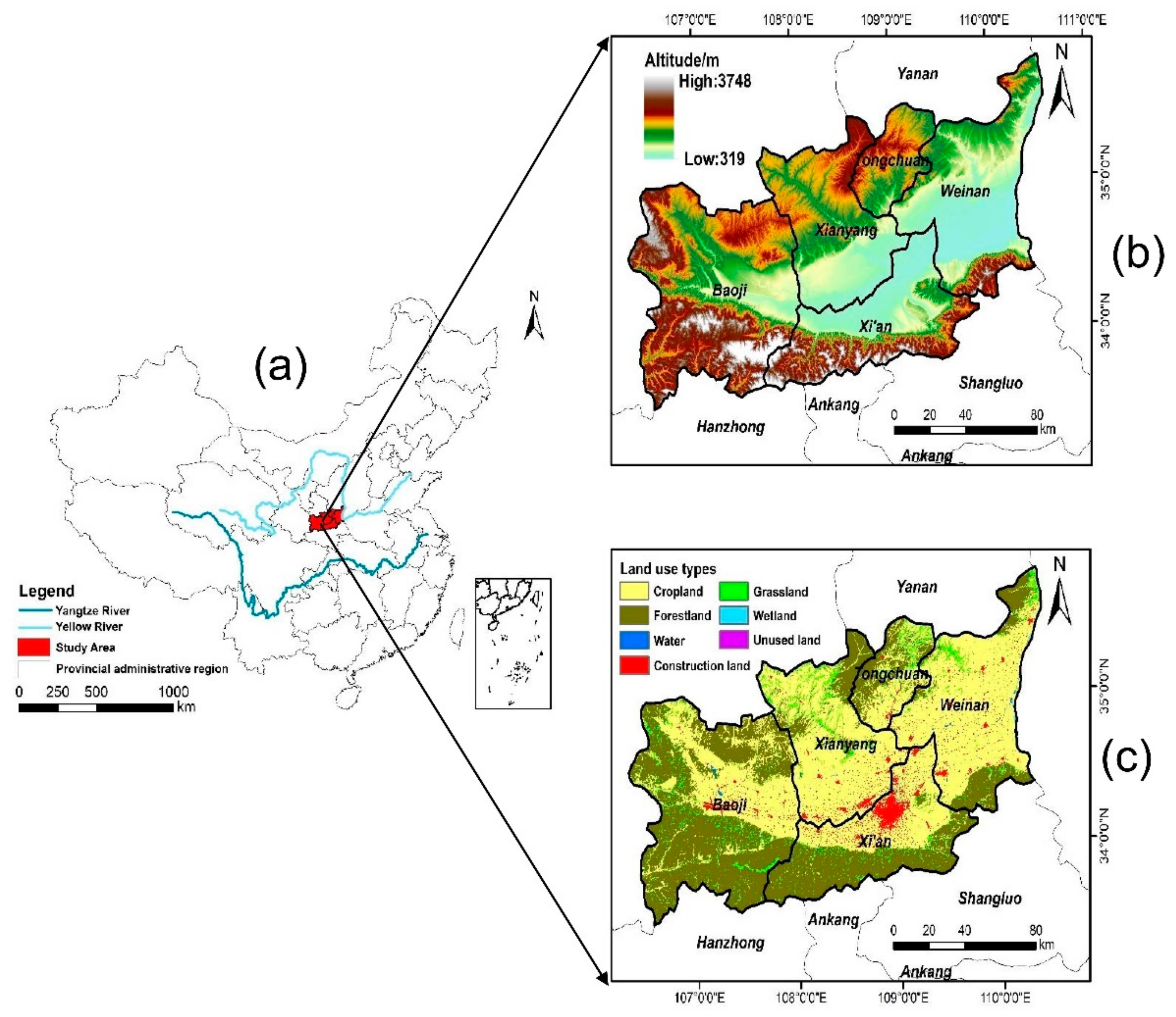
Figure 1. Map of the study area. (a) Location; (b) Altitude; (c) Land use types.
Sustainability 15 07730 g001
Figure 2. The overall technique diagram map.
Sustainability 15 07730 g002
Figure 3. Land-use change in the GZA from 2000 to 2019. (a) Land use spatial transformation map; (b) Chord diagram of land use type transformation.
Sustainability 15 07730 g003
Figure 4. The temporal variations of LCE in the GZA from 2000 to 2019.
Sustainability 15 07730 g004
Figure 5. Temporal dynamics of LCE in different land-use types from 2000 to 2019. (ac) represent the inter-annual trend of carbon sequestration in grassland, wetland and forestland; (d,e) represent the inter-annual trend of carbon emissions from cropland and construction land. “*” Significantly indicating the trend of change (p < 0.05).
Sustainability 15 07730 g005
Figure 6. The level of LCE in the GZA from 2000 to 2019.
Sustainability 15 07730 g006
Figure 7. Spatial dynamics of LCE in the GZA from 2000 to 2019. (a) the spatial variation trend of LCE; (b) Significance test results of change trends based on MK; (c) Superimposed results of spatial change rate and significance test.
Sustainability 15 07730 g007
Figure 8. Spatial clustering features of LCE in the GZA from 2000 to 2019.
Sustainability 15 07730 g008
Figure 9. Correlation of LCE with factors (NTL, PD, and GPP) at global dimension.
Sustainability 15 07730 g009
Figure 10. Spatial distribution patterns of regression coefficients in MGWR.
Sustainability 15 07730 g010
Table 1. Description of data sources used in this study.
Data TypeSpatial Resolution/FormulaSource
Land Use/Cover 300 mEuropean Space Agency (http://maps.elie.ucl.ac.be/CCI/viewer/, accessed on 1 June 2022)
Carbon Emission1 kmOdiac—Fossil fuel CO2 emission data product (http://db.cger.nies.go.jp/dataset/ODIAC/data_policy.html, accessed on 1 May 2022)
Nighttime Light1 kmNOAA website NGDC Data Center
(https://www.ngdc.noaa.gov/eog/download.html, accessed on 4 August 2022)
Population Grid1 kmOpen Spatial Demographic Data and Research—WorldPop
(https://www.worldpop.org/project/list, accessed on 13 August 2022)
Gross Primary Productivity1 kmNational Tibetan Plateau/Third Pole Environment Data Center
(https://data.tpdc.ac.cn/zh-hans/data/582663f5-3be7-4f26-bc45-b56a3c4fc3b7, accessed on 13 September 2022)
Digital Elevation Model (DEM)90 mChina Geospatial Data Cloud (https://www.gscloud.cn/sources/accessdata/305?pid=302, accessed on 10 August 2022)
Table 2. Carbon emission coefficient of land use type (t·hm−2·a−1).
Land Use TypeCarbon Emission Factor
Cropland0.422
Grassland−0.021
Forestland−0.644
Wetland−0.0006132
Unused land−0.005
Water−0.253
Table 3. Statistics of change trend types.
Change TypeDefinition
Significantly increasings > 0, |z| > 1.96
Slightly significantly increasings > 0, |z| < 1.96
No-significantly changings = 0
Slightly significantly decreasings < 0, |z| > 1.96
Significantly decreasings < 0, |z| < 1.96
Note: At the significance level α = 0.05, a significant change occurs when |Z| >1.96, and an insignificant change occurs when |Z| < 1.96.
Table 4. Transfer matrix of land use in the GZA from 2000 to 2019 (km2).
2000CroplandForestlandGrasslandWetlandConstruction LandWaterUnused LandTotal in 2019Transfer in 2019
2019
Cropland33,275.0730.5148.96000033,354.5479.47
Forestland84.623,160.6105.57000023,350.77190.17
Grassland99.27209.523696.840.180004005.81308.97
Wetland00093.7800093.780
Construction land2218.051.62101.432.88440.190.991.262766.422326.23
Water00000104.580104.580
Total in 200035,676.9923,402.253952.896.84440.19105.571.2663675.9
Transfer out in 20002401.92241.65255.963.0600.991.26
Table 5. Global Moran’s I of LCE in the GZA from 2000 to 2019.
YearMoran’s IZ Valuep ValueYearMoran’s IZ Valuep Value
20000.11173.95630.00120100.12444.42250.002
20010.10733.79980.00120110.15665.65950.003
20020.11914.21290.00120120.15665.65810.005
20030.11744.16060.00120130.15655.65450.004
20040.14425.16920.00220140.15655.65740.004
20050.12274.42820.00220150.15625.64710.005
20060.11534.11000.00220160.15705.67460.004
20070.11474.08770.00220170.17556.36890.004
20080.11514.10090.00220180.14135.26220.004
20090.11534.10910.00220190.14135.26180.005
Disclaimer/Publisher’s Note: The statements, opinions and data contained in all publications are solely those of the individual author(s) and contributor(s) and not of MDPI and/or the editor(s). MDPI and/or the editor(s) disclaim responsibility for any injury to people or property resulting from any ideas, methods, instructions or products referred to in the content.