Article

Controlling Industrial Air-Pollutant Emissions under Multi-Factor Interactions Based on a Developed Hybrid-Factorial Environmental Input–Output Model

Fujian Engineering and Research Center of Rural Sewage Treatment and Water Safety, School of Environmental Science and Engineering, Xiamen University of Technology, Xiamen 361024, China
*
Author to whom correspondence should be addressed.
Sustainability 2023, 15(9), 7717; https://doi.org/10.3390/su15097717
Submission received: 22 March 2023 / Revised: 20 April 2023 / Accepted: 25 April 2023 / Published: 8 May 2023

Abstract

:
A hybrid-factorial environmental input–output model (HEIM) is proposed for controlling industrial energy-related air pollution. HEIM has the advantages of analyzing industrial air-pollutant emission system (IAES) performance, quantifying key factors’ individual and reciprocal effects on the system, generating optimal system planning strategies under multiple scenarios. HEIM is then applied to Fujian province, which is a special economic development region in China. The significant findings are as follows: (i) the main sectors of pollutants’ (NOx, SO2, PM and VOCs) emissions are electricity supply (ELE), transportation (TRA), nonmetal minerals (NON), chemical products (CHE) and metal processing (MET); (ii) the proportion of air pollutants (NOx, SO2 and PM) emitted from energy activities can reach 83.8%, 88.6% and 68.1% of the province’s total emissions, implying that it is desired for industrial activities to improve the energy efficiency and promote cleaner production; (iii) the system robustness was between 0.287 and 0.321 (maximum value is 0.368), indicating the emission structure of IAES was not healthy; (iv) the contributions of the key factors to air-pollutant emission equivalent are NOx emission (51.6%) > ELE coal consumption (25.8%) > SO2 emission (12.5%); (v) the contributions of the key factors affecting system robustness are equipment manufacturing’s (EQU) direct consumption coefficient (81.4%) > CHE coal consumption (11.7%) > NON coal consumption (5.0%). The optimal strategies should strictly control ELE coal consumption (replaced by clean energy) and strictly limit NOx and SO2 emissions (e.g., technology upgrade) from the main sectors.

1. Introduction

1.1. Importance and Motivation

The world has undergone rapid economic development and population growth as well as accelerating industrialization and urbanization, which has also led to serious environmental pollution [1]. For China, the emissions of sulfur dioxide (SO2), nitrogen oxides (NOx) and particulate matter (PM) reached 18.6 × 10⁶, 18.5 × 10⁶ and 15.4 × 10⁶ tons in 2015; the shares of SO2 and NOx were more than 30% and 20% of global emissions [2,3]. In 2017, only 30% of China’s cities met the National Ambient Air Quality Standard, with non-compliance of PM being the most prominent air pollution problem [4]. The Global Burden of Disease report indicated that China is one of the top two countries for premature deaths associated with air pollution, with 1.2 million deaths in 2017 [5]. Furthermore, air pollution has caused huge economic losses, equivalent to 1.2% of China’s annual gross domestic product (GDP) based on disease costs and 3.8% of annual GDP based on willingness to pay [6]. Reducing air-pollutant emissions is a great challenge for the Chinese government in the 21st century.
Fossil energy combustion (e.g., coal and oil) for economic production activities is the main source of air-pollutant emissions [7]. Due to differences in sectoral energy consumption, the emission performance of various economic sectors varies significantly [8]. A sector usually emits multiple air pollutants at the same time, and various pollutants have different hazards due to different generation mechanisms. In addition, the generation of emissions can be indirectly induced through intersectoral trade [9]. Many factors, such as sectoral energy consumption structure, emission types and intersectoral trade, jointly affect the regional air security. Such complexities would correspondingly bring more challenges to mitigate air pollution [3,10]. It is essential to quantify such complexities for decision makers to formulate reliable control strategies adopting more robust system analysis methods.

1.2. Literature Review

To seek effective emission reduction strategies from a socio-economic perspective, the production-based approach (PBA) and consumption-based approach (CBA) are widely employed for accounting the emissions of air pollutants [9,11]. PBA can restrain the air-pollutant emission behavior of producers and can facilitate producers to improve the energy efficiency of unit products [12]. Many scholars, based on PBA, analyzed the generation mechanism of air pollutants and developed advanced cleaner production technologies [13,14]. For example, Mozaffar et al. [15] measured the concentration levels of NOx, SO2, volatile organic compounds (VOCs), ozone (O3) and carbon monoxide (CO) in the City of Nanjing and investigated their effects on the formation of O3. Zwolińska et al. [16] developed an integrated method to remove NOx and SO2 from diesel off-gases simultaneously. Moreover, in order to analyze and simulate regional air quality, a series of air pollutants (e.g., NOx, SO2, PM, VOCs and CO) emission inventories were established [17,18]. However, PBA ignores the existence of indirect emissions caused by sectoral production activities in the supply chain, which can lead to pollution spillovers and affect the effects of mitigation policies. Excluding indirect emissions can essentially lead to inequitable distribution of emission control assignments, further affecting regional emissions control efficiency, and this can adversely affect active involvement in emission control.
Compared to PBA, CBA measures air-pollutant emissions from final products (and imports), where responsibility for air-pollutant emissions control is taken by users. In terms of CBA, an environmental input–output model (EIOM) provides a powerful tool to assess direct and indirect emissions by considering intersectoral commodity trade and final consumption [19,20]. In EIOM, the traditional economic system is converted into an industrial air-pollutant emission system (IAES). EIOM has been widely employed to support the reduction of various air pollutants. Specifically, Alcántara et al. [19] applied EIOM to calculate NOx emission of different sectors in Spain; the results provided guidance for different sectors to formulate corresponding NOx emission reduction strategies. Yang et al. [21] used EIOM for analyzing the transfer of embodied PM2.5 emissions in north China, which revealed that the embodied PM2.5 exports from the north China region mainly flows to China’s central coastal areas and the Beijing–Tianjin region. Liu et al. [22] employed EIOM to analyze the driving factors of SO2 emissions in 30 provinces of China, where domestic final demands, domestic exports and international exports were screened out. Li et al. [23] determined the flow patterns of PM2.5 emission in the Beijing–Tianjin–Hebei region through EIOM; the results showed that Beijing is a net importer and Hebei is a net exporter of PM2.5. Zhang et al. [24] used EIOM to investigate the changes in air pollutant emissions among various sectors in China from 2012 to 2017; the results indicated that the metal sector replaces the power sector as the largest net emitter. Bortoli and Agez [25] developed an EIOM for analyzing the industrial environmental impacts of Canada, where the main sectors were recognized depending on a comprehensive indicator, and strategy adjustments were suggested (e.g., reducing concrete and asphalt products and increasing investment in machines powered with clean energies). These proved that the EIOM can reveal IAES performance and calculate emission amounts, analyze emission flows, explore intersectoral relationships and detect system robustness.
When considering the city as a “superorganism” in nature, various socioeconomic factors are directly and/or indirectly linked [26]. IAES can be treated as a network where economic sectors are analogous to nodes and inter-sector transactions are analogous to edges. According to complex network theory, there are socioeconomic factors that are critical to reducing emissions. An IAES can be likened to a network where economic sectors are nodes and inter-sector transactions are edges. According to complex network theory, there are socioeconomic factors (e.g., multiple sectors, energy sources, air pollutants, treatment measures and reaction processes) that are critical to reducing emissions. These factors may be featured with uncertainty and interact with each other, leading to plenty of interactions hidden in IAES [27]. For example, changes in the production capacity of the metal manufacturing sector can affect the transmission of electricity in the power sector and the mining of metal minerals in the mining sector. EIOM can effectively classify sectors as direct emitters or indirect emitters to allocate different emission responsibilities; however, it cannot effectively identify the factors and their interactions that have a key impact on emission reductions. Such ignorance may hinder the authorities in making sound pollution control strategies.
An attractive method that can be used to address the above-mentioned obstacles is factorial analysis (FA), which can quantify the individual and reciprocal effects of factors on system responses [28,29]. Liu et al. [30] employed FA for exploring greenhouse gas types and sources’ effects on urban emission systems in Saskatchewan, where the effects of individual factors and interactions were quantified. Wang et al. [29] proposed an FA-based multivariate statistical prediction method to investigate the variation of the Guangzhou–Foshan region forest coverage area, which effectively revealed the potential relationship between human activity and natural factors. Zhang et al. [31] used FA to analyze the interactions of temperature, oil type, gas composition, gas-oil ratio and pore radius on the interfacial tension and minimum miscibility pressure of the light oil–CO2 system. Jia et al. [32] employed FA to explore the effects of human activity and hydrological and ecological factors on inflow from the Syr Darya to the Aral Sea; the results revealed that agricultural water consumption was the most important factor. The above-mentioned studies are effective in exploring the effects of a small number of factors. FA may be infeasible when facing a great number of factors, due to the massive amounts of times required of running the model [33]. A hybrid-factorial analysis (HFA) method can be formulated to handle these problems. Taguchi analysis is employed to screen key factors by performing only a fraction of the total number of running times. Full factorial analysis including these factors can be employed to explore their reciprocal effects on IAES performance, and optimal industrial air-pollutant emissions control strategies can be obtained by introducing a commonly used selection method.

1.3. Objective and Contribution

Based on previous research, this study aims to put forward a hybrid-factorial environmental input–output model (HEIM) for controlling industrial energy-related air pollution. The main contributions are as follows: (i) this is the first attempt to develop such a new HEIM for an industrial air-pollutant emission system (IAES); (ii) the model cannot only identify the main industrial sectors and crucial paths of multiple pollutants’ emissions, but can also reveal the associated relationships among sectors and the emission status in IAES; (iii) the model can also calculate the contributions of multiple factors’ variation to IAES’s emissions, flows, forces and robustness changes for exploring key factors and their interactions; (iv) an entropy-based TOPSIS method is introduced for screening and generating optimal industrial air-pollutant emission control strategies. HEIM is applied to support IAES planning of Fujian province to verify its feasibility and practicality.

2. Methodology

HEIM is formulated through introducing the HFA method into an EIOM framework (details are in Figure 1). In the model, NOx, SO2, PM and VOCs are generated from coal, gasoline, diesel, kerosene and fuel oil. EIOM reveals the performance of IAES and recognizes the main sectors. HFA screens out the key factors by Taguchi analysis and gains insight into the interactions between key factors by full factorial analysis. The entropy-based TOPSIS method provides final decision-making support (details are listed in Supplementary Material).

2.1. Environmental Input–Output Model

An input–output model (IOM) is used to reveal the interdependent economic relationships between various sectors [34]. In the input–output table (IOT) of IOM, the horizontal direction represents where the output of the sector is consumed, and the vertical direction indicates the input source required by the sector for production activities. The physical IOM can be developed by introducing embodied environmental element intensity into conventional IOM, which is useful for reflecting the overall status of air-pollutant emissions through sectoral monetary transactions [35]. It can be presented as follows:
X i = j = 1 N Z i J + f i
E + ε Z = ε X
ε = E ( X Z ) 1
E N a p = d i a g ( ε ) Z
D E t , i = p = 1 C S i , p × E C t , i , p
E i = t = 1 ( D E t , i / S C t )
where i and j represent the economic sectors in the IOT; Xi is the economic sectoral output, X = diag(Xi)N×N; Zij is the use of product i assigned to sector j, Z = [Zij]N×N; fi is the sectoral final demand; E indicates the air-pollutant emission equivalent (APEE) of a sector, which is used to comprehensively reflect the environmental hazards of different air pollutants, E = [Ei] N; ε represents the embodied environmental emission matrix (ε = [εi] N, εi represents the emission coefficient of air pollutants form embodied in the products of a sector); ENap is the flow of air pollutants between sectors; DEt,i is the emission of the air pollutant t from sectoral energy consumption; CSi,p is the fuel, p, consumption by sector i; ECt,i,p is the emission coefficient; SCt is the pollution equivalent value of air pollutant, t.
IAES can be constructed through Equation (7) to further analyze each kind of air pollutant flow into or out of each sector [36]. Because there are different air-pollutant emission flow paths between sectors, the non-dimensional integral air pollutant emission matrix, N, can be computed by Equations (8) and (9). The matrix, Yap, which represents the integral air-pollutant emission flow between sectors, can be calculated as follows:
T i a p = j = 1 n E N j i a p + E i
g i j = E N i j a p / T j a p
N = ( G ) 0 + ( G ) 1 + ( G ) = ( I G ) 1
Y a p = d i a g ( T a p ) N
where T i a p represents the total air-pollutant emissions of sector i, including inflows from other sectors and self-emissions; gij is the dimensionless air pollutant emission coefficient from sectors i to j; Gn is the dimensionless air pollutant emission intensity matrix, with n path lengths.
To reflect the influence of the input and output integral air pollutant flow of one sector on the IAES, the driving force and pulling force indicators are introduced [37]:
W i = j = 1 n y i j a p / i = 1 n j = 1 n y i j a p
W j = i = 1 n y i j a p / i = 1 n j = 1 n y i j a p
where y i j a p represents the integral air pollutant flow from sectors i to j; Wi is the sectoral driving force; Wj is the sectoral pulling force.
In IAES, there are various emission paths with different intensities. When emissions within the system are concentrated and in a limited path, it will show higher efficiency and organization but will also be vulnerable to external disturbances. When emissions are uniformly distributed, the system will show higher redundancy and be more resilient to perturbations. According to ecological network theory, efficiency and redundancy are significant indicators to characterize the health of the emission system [38]. The comprehensive indicator (i.e., robustness) can measure the tradeoff relationship between them, and it can reflect the health condition of IAES. Robustness (R) is obtained as follows [39]:
Efficiency:
A M I = K i j ( E N i j a p i j E N i j a p ) log ( E N i j a p i j E N i j a p i E N i j a p j E N i j a p )
Redundancy:
H c = K i j ( E N i j a p i j E N i j a p ) log ( E N i j a p 2 i E N i j a p j E N i j a p )
Robustness:
R = [ A M I / ( A M I + H c ) ] log { [ A M I / ( A M I + H c ) ] }
Generally, indicators of E, Yap, W and R reflect the emission intensity, emission path, intersectoral relationship and emission status in IAES, respectively.

2.2. Hybrid-Factorial Analysis

2.2.1. Taguchi Analysis

Taguchi analysis is an efficient experimental design method to identify factors that have an impact on system performance. It contains certain standard orthogonal arrays (a number of fixed designed matrix) to evaluate multiple factors’ independent influence in a minimum number of calculation scenarios [40]. Each column in the matrix represents a design factor, and each row represents an experiment with a combination of different design factor levels. Response values under different scenarios are transformed into signal to noise (S/N) ratio. This is used to calculate the deviation between the expected and the test results to explore the ability of factors to affect the variability of the response. S/N ratio is divided into three types, out of which the appropriate type should be selected based on the response target. The S/N ratio can be obtained by:
(1)
Larger the better (i.e., selected when the target maximizes the response).
S / N = 10 l o g ( ( 1 / Y i 2 ) / n )
(2)
Smaller the better (i.e., selected when the target minimizes the response).
S / N = 10 l o g ( ( Y i 2 ) / n )
(3)
Nominal the better (i.e., selected when the target is the response itself and the S/N ratio is based on the standard deviation only).
S / N = 10 l o g ( ( Y i Y 0 ) 2 )
where Yi is the response value of the ith computation; n is the number of computations; Y0 is the mean of all response values.

2.2.2. Full Factorial Analysis

Taguchi analysis can effectively identify key factors, but it cannot fully reflect the interaction among these factors [41]. Some interactions that differ from the effects of a single factor may be important. Full factorial analysis is adopted to detect the joint effects of selected factors [42]. 2k factorial analysis is a commonly used method, where each factor is divided into low (L) and high (H) levels, resulting in 2k (for k factors) treatment combinations. The summation of the squares of individual factors and two factors’ combination can be computed as follows:
S S a = 1 V W u = 1 U ( v = 1 V w = 1 W Y u v w ) 2 1 U V W ( u = 1 U v = 1 V w = 1 W Y u v w ) 2
S S b = 1 U W v = 1 V ( u = 1 U w = 1 W Y u v w ) 2 1 U V W ( u = 1 U v = 1 V w = 1 W Y u v w ) 2
S S c = 1 U V w = 1 W ( u = 1 U v = 1 V Y u v w ) 2 1 U V W ( u = 1 U v = 1 V w = 1 W Y u v w ) 2
S S a × b = 1 W u = 1 U v = 1 V ( w = 1 W Y u v w ) 2 1 U V W ( u = 1 U v = 1 V w = 1 W Y u v w ) 2 S S a S S b
S S a × c = 1 V u = 1 U w = 1 W ( v = 1 V Y u v w ) 2 1 U V W ( u = 1 U v = 1 V w = 1 W Y u v w ) 2 S S a S S c
S S b × c = 1 U v = 1 V w = 1 W ( u = 1 U Y u v w ) 2 1 U V W ( u = 1 U v = 1 V w = 1 W Y u v w ) 2 S S b S S c
where a, b and c denote input factors; U, V and W represent the number of levels of each factor; Yuvw represents the response value at level u, v and w of factor a, b and c, respectively; SSx and SSx×y represent the summation of squares of individual factors and two factor combinations.

3. Case Study

3.1. Statement of Problem

Fujian, a coastal province in East China, has been on the fast lane of extensive economic development as a spearhead in the country’s reform and opening up. Fujian’s GDP increased 661 times from 1978 to 2020, with an average annual growth of approximately 12%. In 2020, Fujian’s GDP reached RMB¥ 4.39 trillion, occupying 4.3% of the whole country (ranking 7th in China). Rapid economic growth demands more energy, but this situation exacerbates regional air pollution. From 2015 to 2019, Fujian’s energy consumption increased by 18.9%. In 2015, the emissions of NOx, SO2 and PM in Fujian reached 337.9 × 10³, 379.9 × 10³ and 341.7 × 10³ tons, respectively [43]. These pollutants have caused a series of environmental problems such as increased ozone concentration, acid rain pollution and haze. As China’s first national ecological conservation pilot zone, Fujian’s goal is to achieve a green development pattern and establish a comprehensive ecological environment control system by 2035, while its industrial structure is still in a high energy consumption pattern and relies heavily on fossil energy consumption. The local government urgently needs to seek emission reduction and cleaner production strategies to support its sustainable development.

3.2. Data Collection

The input–output table (IOT) of Fujian province containing 42 sectors were extracted from the Fujian Statistics Bureau, and the IOTs for 2012 and 2017 are the latest available data. Recent Fujian Statistical Yearbooks show that the provincial economic structure has no obvious change. The proportions of primary, secondary and tertiary industries were 7%→6%, 49%→46% and 44%→48% (“→” denotes tend) in the most recent five years, respectively. The energy consumption structure also barely changes. Secondary industry was the largest energy user (i.e., accounting for more than 67% of total energy consumption). The 42 sectors in the original table are merged into 16 sectors according to the Industrial Classification for Nation Economic Activities (GB/T 4754-2017) and energy consumption data (in Table 1). The sectoral emission coefficients and energy consumption were obtained from the Fujian Statistical Yearbook, China Energy Statistical Yearbook, and official websites and the literature [43,44,45].

3.3. Scenario Design

Based on the analysis results of Fujian province in 2012 and 2017 using EIOM, the main direct and indirect emission sectors can be recognized. Then, HFA is conducted using the following steps: (1) select the energy consumption of the main sectors, direct consumption coefficient of the main sectors and sectoral pollutant emission coefficients as factors, and divide them into two levels; (2) choose the indictors of APEE and robustness as responses; (3) choose the appropriate orthogonal array Lx (e.g., L27, L32) by the factors and their levels, leading to Lx scenarios; (4) run EOM to obtain a set of response values under all scenarios; (5) calculate the S/N ratios to identify k key factors (i.e., those with 90% of contribution); (6) calculate summation of squares of k factors based on response values under 2k scenarios. Finally, the entropy-based TOPSIS method is used to help generate optimal scenarios for supporting the regional industrial air-pollution control. According to Fujian province’s 14th Five-Year (2020–2025) energy conservation and emission reduction comprehensive work plan, the high level of the selected factors is maintained at the 2017 value, and the low level is reduced by 20%. The sectoral emission pollutant coefficients are divided according to strict and loose environmental policies (in Table 2).

4. Result and Discussion

4.1. Air Pollutant Emissions

Figure 2 depicts air pollutants emitted from various sectors. In 2012, the emissions of NOx, SO2, PM and VOCs related to sectoral energy activities reached 306.1 × 10³, 258.9 × 10³, 159.4 × 10³ and 26.3 × 10³ tons. Among them, the shares of NOx, SO2 and PM were more than 65.5%, 69.8% and 63.0% of the province’s emissions. The emissions of these four pollutants reached 232.3 × 10³, 118.7 × 10³, 115.6 × 10³ and 18.2 × 10³ tons in 2017, and the emissions of NOx, SO2 and PM accounted for 83.8%, 88.6% and 68.1% of the total emissions, respectively. Compared with 2012, the proportion of pollutants emitted from sectoral energy activities increased significantly, indicating that energy consumption became the most important cause of local air problems. For sectoral emissions, ELE, TRA, NON, CHE and MET dominated various emission in both years. In 2012, these five sectors contributed 85.3%, 89.5%, 89.4% and 77.7% to NOx, SO2, PM and VOCs emissions. In 2017, the emissions of these sectors occupied 87.1%, 84.6%, 88.1% and 71.2%, respectively. The results imply that adjusting energy consumption structure and improving the use efficiency of these energy-intensive sectors can reduce pollutant generation.
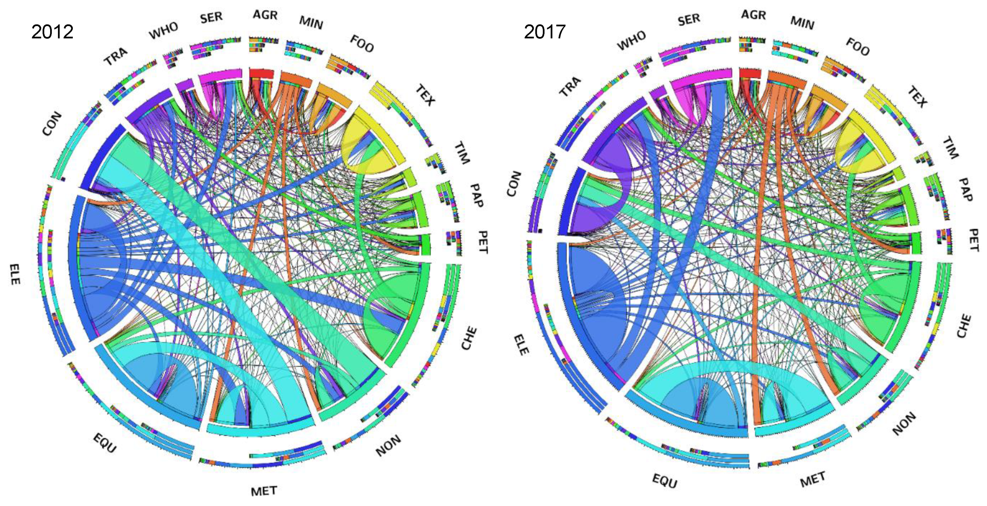
Figure 3 presents the flow of APEE among sectors. Each sector matches a specific color; the line between sectors indicates the direction of APEE flow, and the width of the line indicates the amount of inflow or outflow. It is shown that the flow of APEE among sectors in 2017 is similar to that in 2012. The largest contributor of APEE flow was ELE, occupying 21.9% (in 2012) and 19.7% (in 2017) of the total flow. ELE remained irreplaceable in terms of supplying energy to other sectors. The largest recipients were CON and EQU, which together accounted for 30.6% (in 2012) and 28.6% (in 2017) of the total flow. This is because these two sectors mainly receive emissions from the upstream sector (e.g., MET and NON) that produces raw materials for them. It is worth noting that, in 2017, TRA replaced MET and NON as the largest contributor to CON. ELE reduced the inflow to the advanced manufacturing industries (e.g., CHE, NON and MET) and increased the inflow to SER and TRA. This is because the local government has increased its investment in tertiary industry since 2012, with more resources such as electricity and heat tilted toward it.
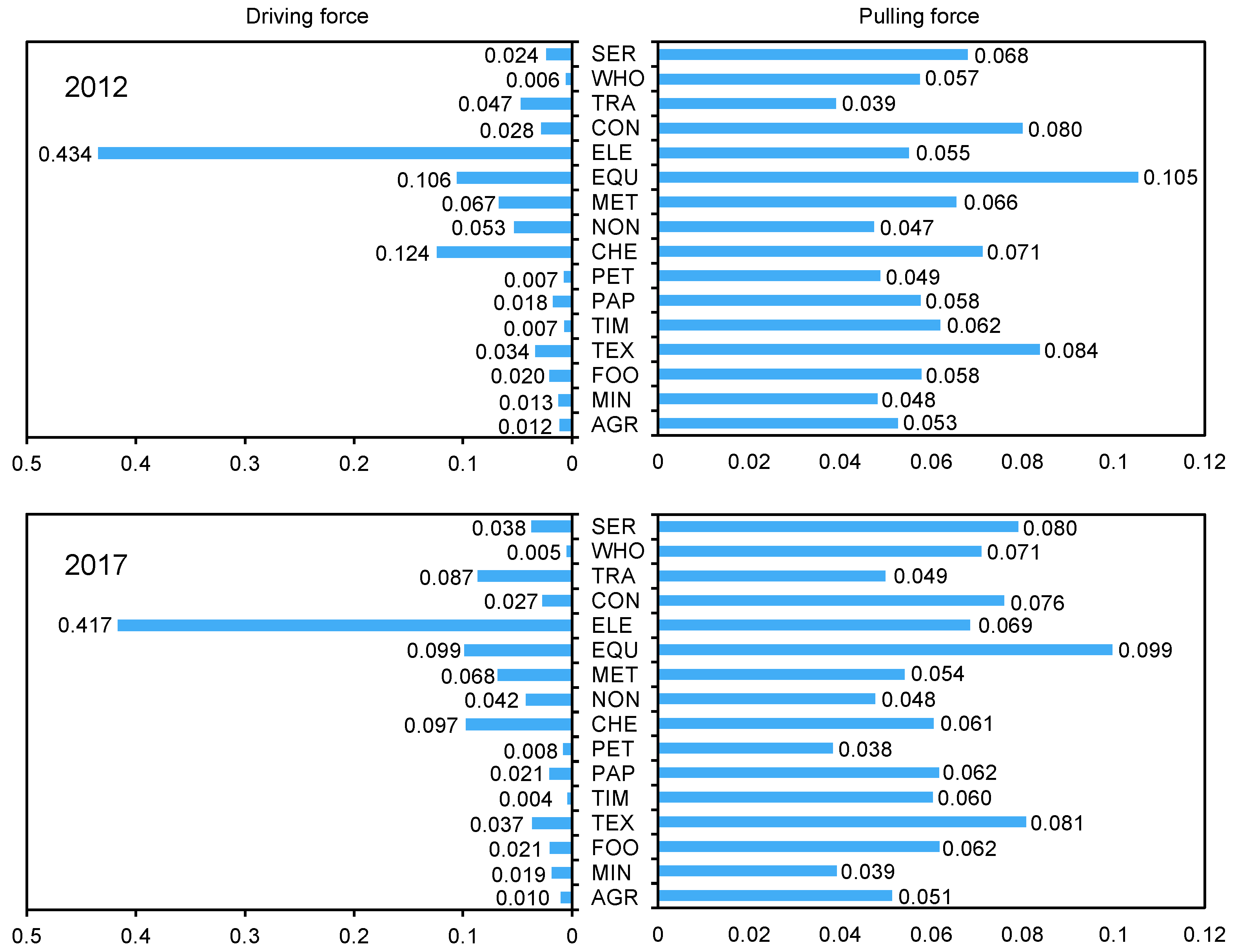
Figure 4 presents the sectoral driving and pulling forces. The results show that ELE has the highest driving force (0.434 in 2012 and 0.417 in 2017), followed by CHE (0.124 in 2012 and 0.097 in 2017) and EQU (0.106 in 2012 and 0.099 in 2017). These indicate that they deliver high amounts of air pollutants to other sectors. Energy-related products (e.g., electricity, fertilizer and metal products) are regarded as outputs from the three sectors to others, leading to their high driving force. Reducing these sectors’ driving forces can help reduce air-pollutant emissions, such as adopting alternative energy (e.g., wind, solar and nuclear power). The total pulling force of EQU, TEX, CON and SER were high (0.337 in 2012 and 0.336 in 2017), indicating that they have strong capacity to receive air pollutants. This is because the production of commodities in these sectors depend on the supply of raw materials (e.g., steel, plastic, ceramic) from upstream emission-intensive sectors. Compared with 2012, the pulling force of these sectors had no obvious changes. It is imperative to adjust their demands (i.e., reducing direct consumption of previous raw materials) to reduce upstream emissions by seeking cleaner production alternatives.
The structure characteristic of IAES was diagnosed by a robustness curve. As shown in Figure 5, the system robustness values in 2012 and 2017 were 0.287 and 0.321, respectively, indicating that the efficiency of IAES has increased to a certain extent. Robustness values are on the left side of the curve and are much smaller than the maximum value (i.e., 0.368). This shows that IAES was in a state of high redundancy and low efficiency. The redundancy for both years was 2.087 and 2.656, which were 5.5 and 4.1 times the corresponding efficiency. Higher redundancy represents a more stable system and the ability to withstand external disturbances. This is beneficial to the natural ecosystem, but very detrimental to pollution control. Higher redundancy means APEE flows more spread out instead of concentrating in a few paths, making the key sectors for controlling air pollution more difficult to determine. Generally, the emission structure of IAES was not healthy due to high redundancy. Further identifying these key influencing factors to formulate more targeted control strategies is essential.

4.2. Identification of Key Factors

Seventeen factors (Table 3) were designed to explore their impact on IAES. L32 (217) orthogonal arrays were selected, and 32 scenarios were obtained correspondingly, as shown in Table S1. Figure 6 depicts the amount and composition of APEE under Taguchi analysis. The results showed that the APEE amount ranges from 286.6 × 10⁶ (under S1) to 374.9 × 10⁶ (under S31), revealing that the designed factors are effective in reducing air-pollutant emissions. Under all scenarios, NOx emissions contributed the highest to APEE, ranging from 56.6% (under S29) to 65.2% (under S20), followed by SO2 contribution from 27.8% (under S19) to 35.9% (under S30). This means that the most significant pollutants causing air pollution are NOx and SO2. Emission reduction should focus on reducing the emissions of these two pollutants. The results also indicated that the contribution of coal to the emission of various air pollutants is much greater than that of other energy types, ranging from 64.1% (under S7) to 71.0% (under S30). For example, the contribution of gasoline, diesel and kerosene under S19–21 has obviously changed, but it is still far smaller than that of coal. This is attributed to the huge use of coal and coal is more likely to generate emissions. It is essential to reduce Fujian’s dependence on coal consumption.
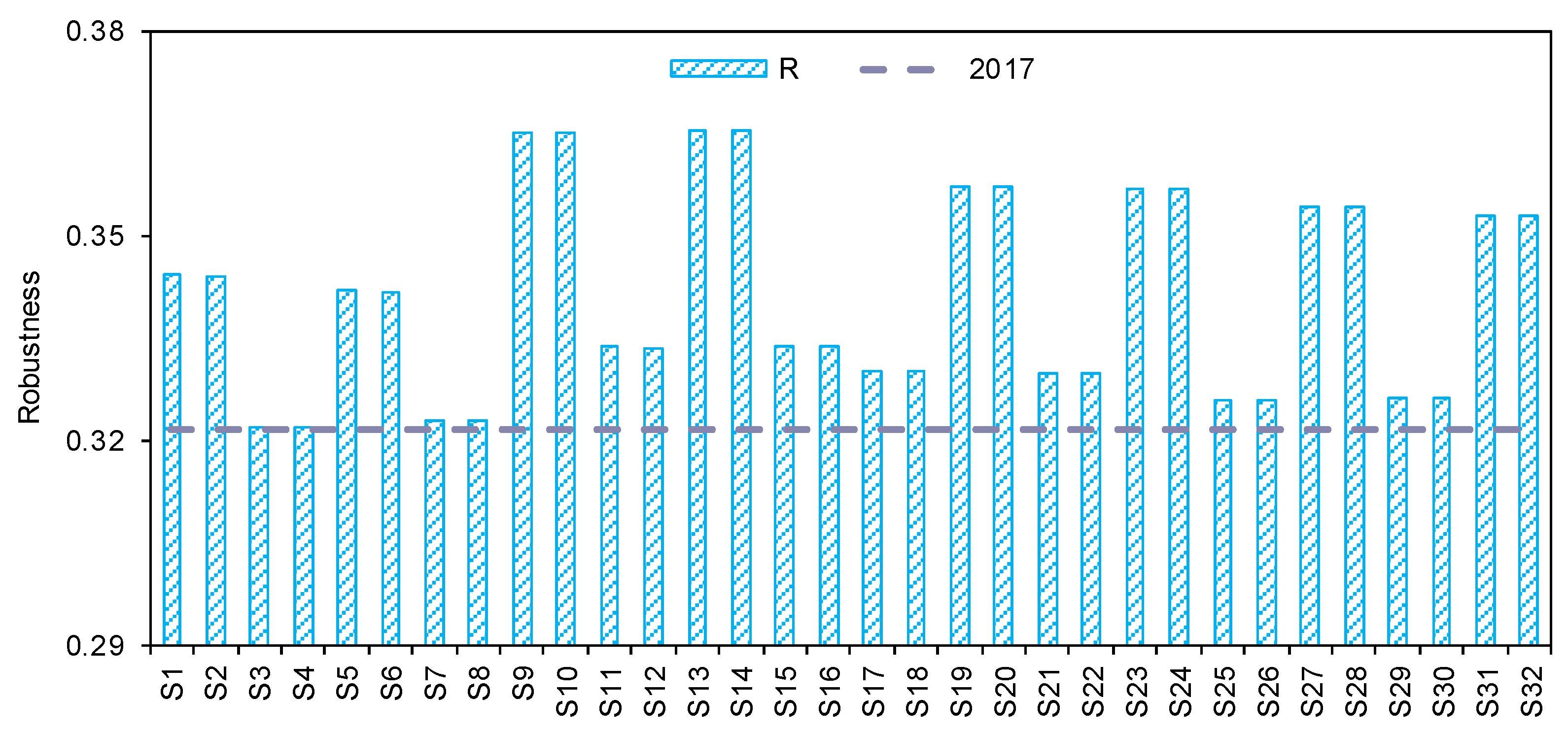
Figure 7 presents the robustness of IAES under Taguchi analysis. Results showed that robustness values range from 0.322 (under S4) to 0.365 (under S13). All robustness values are greater than 2017, and the values under S9, S10, S13 and S14 are close to the maximum robustness. The results illustrate that the efficiency of IAES can be improved through reasonable adjustment. For example, the efficiency of IAES under S13 has improved by 60.1% compared to 2017, while the redundancy has decreased by 17.8%. The increased efficiency means that emissions would become concentrated, which would contribute to achieving emissions mitigation. The fluctuation of values under different scenarios implies that the effect of the designed factors on the robustness varies significantly. It is crucial to identify the key factors affecting robustness.
Table 4 and Table 5 display the S/N ratio of designed factors to APEE and robustness. Factors with higher delta value of S/N (maximum value—minimum value) response indicate more significant effect. Results showed that for APEE, NOx has the largest effect followed by ELE_coal and SO2. This means that APEE would be sensitive to the changes in NOx and SO2 emission coefficients, and the coal consumption of ELE. These results may be related to the production characteristics of sectors. ELE relates to active transactions with other sectors, consuming large amounts of coal to meet the needs of others for essential services such as electricity, gas and water supply; in addition, the combustion of coal is more likely to result in the emission of large amounts of harmful gases such as NOx and SO2. The robustness results showed that EQU_a has the largest effect followed by CHE_coal and NON_coal. The most important factor affecting system robustness was EQU_a, indicating that the direct consumption coefficients of EQU dominated the concentration of emission flows. EQU should improve resource utilization efficiency and optimize the supply structure of production factors.
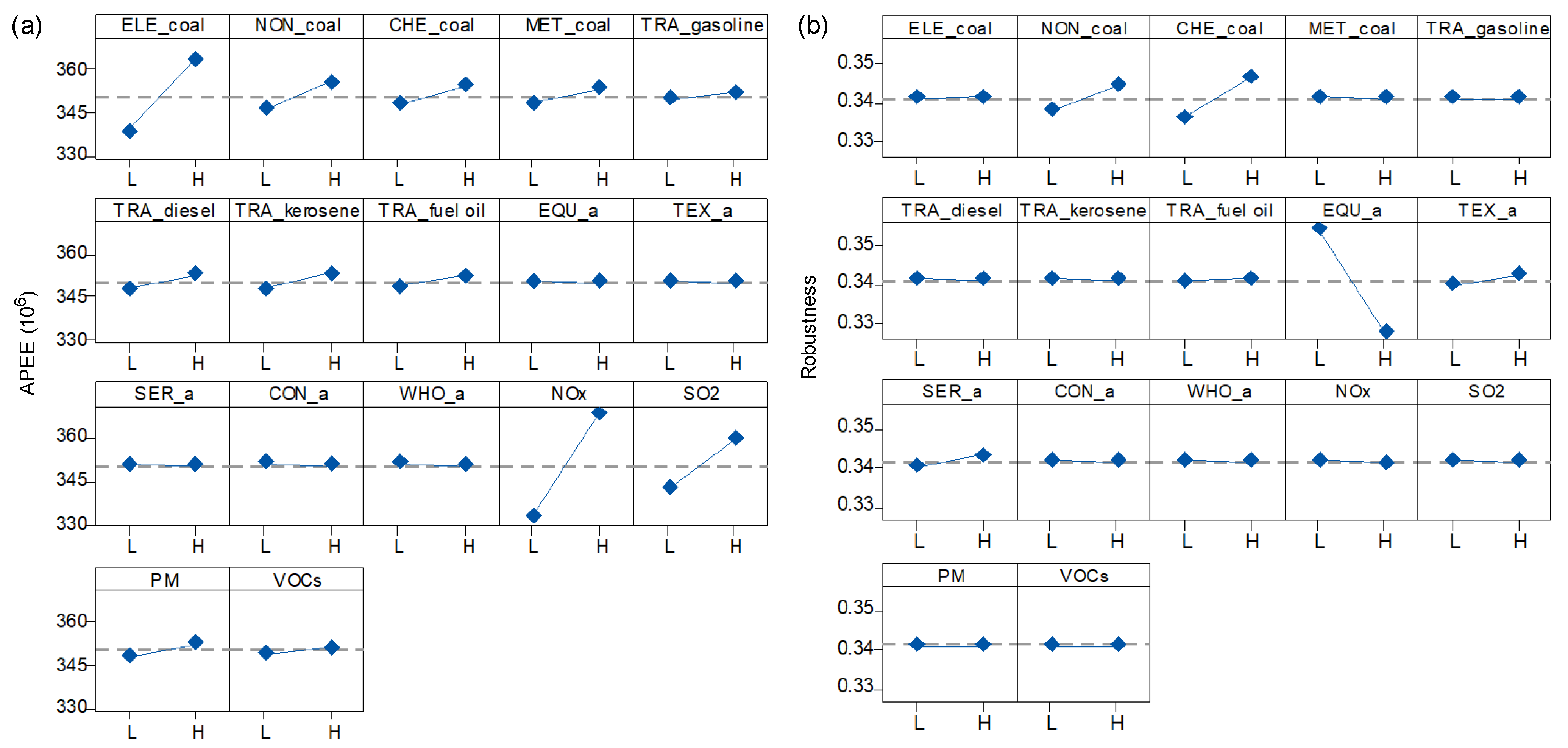
Figure 8 shows the main effects of design factors on APEE and robustness. It is shown that NOx, SO2 and ELE_coal have obvious positive effects on APEE, with 89.9% of contribution to the APEE variation. Taking the plot of NOx as an example, APEE increases from 331.8 × 10⁶ to 368.7 × 10⁶, with NOx increasing from its L level to its H level. NOx has the steepest slope, indicating that it is the most influential (with a contribution of 51.6%) factor. To reduce Fujian’s APEE, the most effective way is to reduce the increment of positive impact factors, such as reducing coal consumption in ELE and reducing NOx and SO2 emission coefficients. The robustness results indicate that EQU_a has obvious negative effects (contribute 81.4%), while CHE_coal and NON_coal have obvious positive effects (contribute 11.7% and 5.0%, respectively). Therefore, the most effective way to improve the robustness is to reduce the direct consumption coefficient of EQU (i.e., reducing reliance on materials with high emissions) and to increase the coal use in CHE and NON. Based on the delta value and the main effects of factors, ELE_coal, CHE_coal, NON_coal, EQU_a, NOx and SO2 were identified as key factors, and other factors were excluded from further analysis.

4.3. Determination of Optimal Strategies

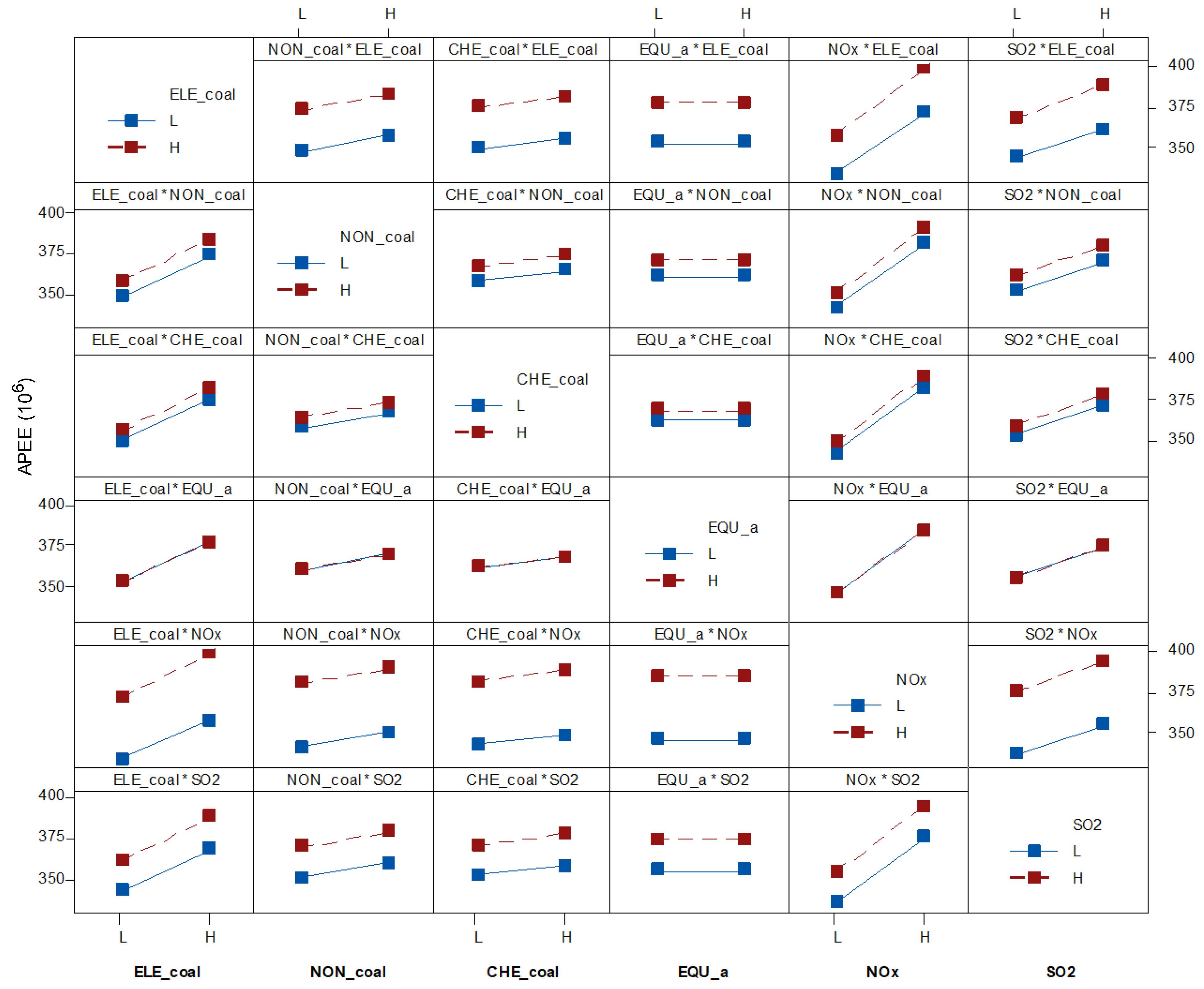
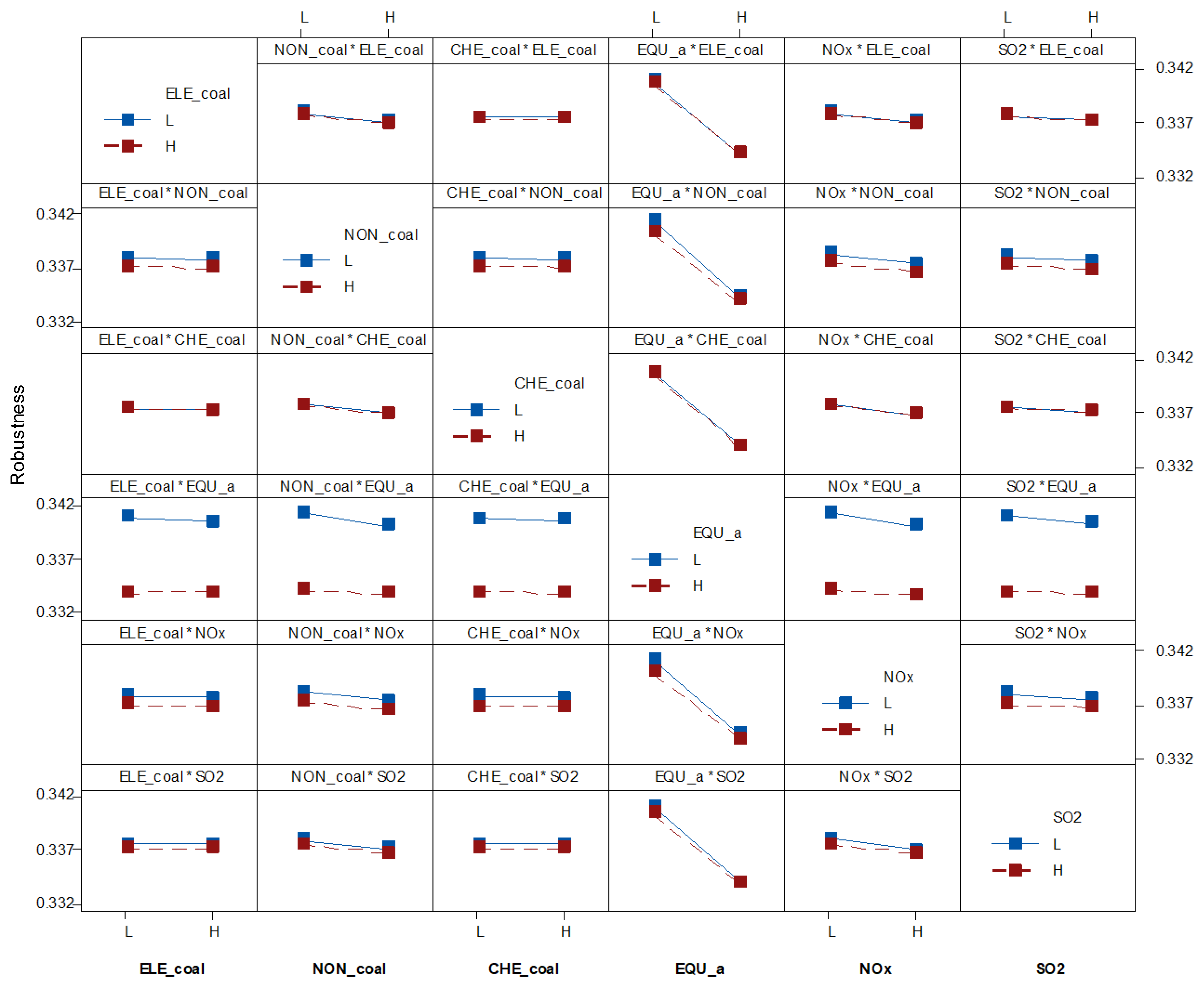
Based on the aforementioned analysis, 26 combinations (i.e., the 64 scenarios in Table S2) can be deigned and used to explore their interactions on IAES’s APEE and robustness by calculating their summation of squares. Figure 9 shows the reciprocal effects of key factors on APEE. It is shown that NOx would interact with ELE_coal, NON_coal and CHE_coal; SO2 would have interactions with ELE_coal, NON_coal and CHE_coal. This indicates that end-of-pipe treatment technologies and sectoral energy consumption can affect each other when implementing direct emission reduction strategies. Figure 10 shows the reciprocal effects of key factors on robustness. It is shown that EQU_a would interact with ELE_coal, NON_coal, NOx and SO2. This is because the raw materials required for EQU production are mainly supplied through the consumption of coal in ELE and NON. This shows that optimizing emission paths in IAES requires coordinated development of upstream and downstream sectors to reduce excessive flows of intermediate products in other sectors. The complex interactions between different factors can jointly affect air-pollution control of the entire region, and this is an inescapable finding.
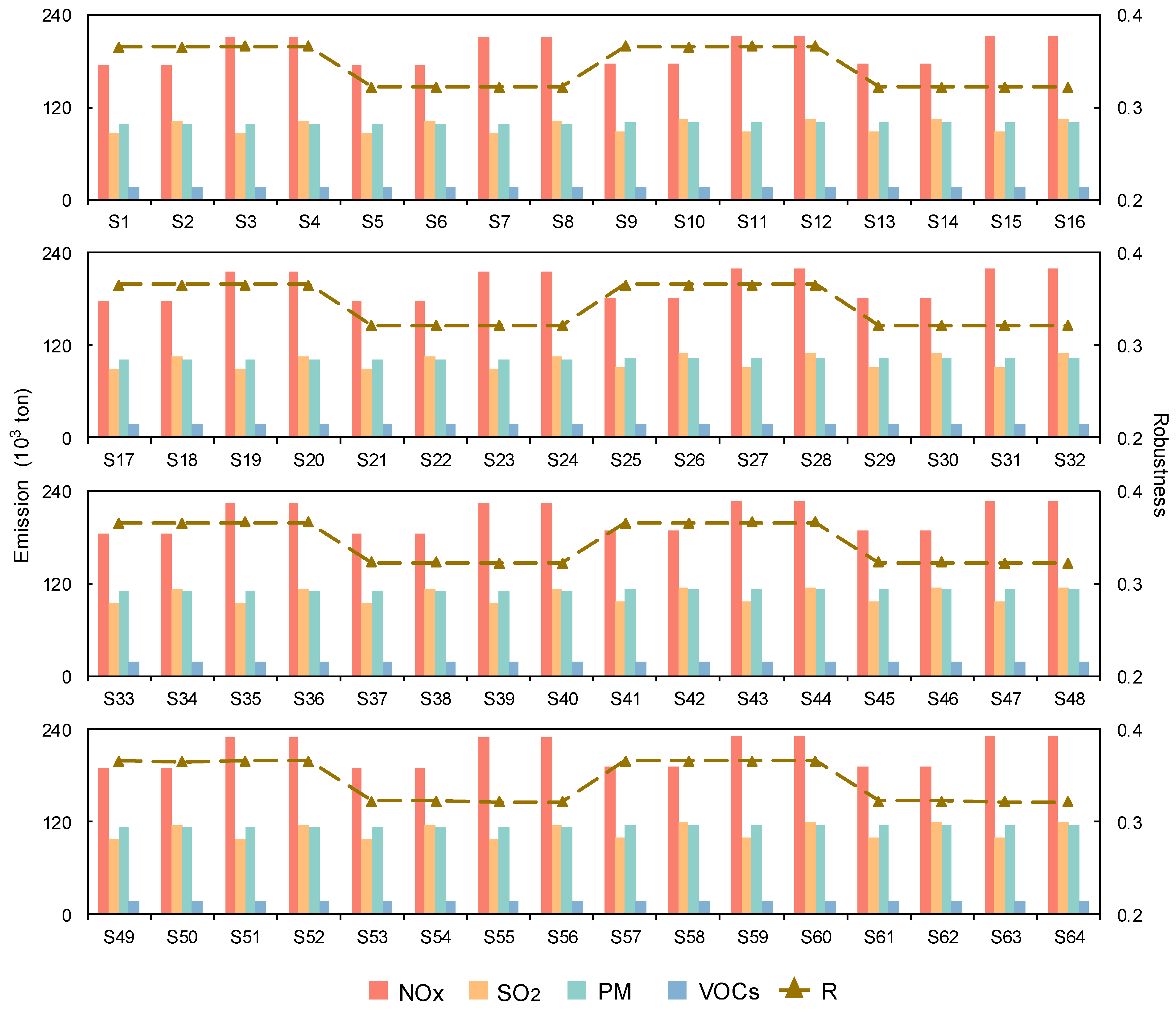
Figure 11 shows the emissions of four air pollutants and system robustness under 64 scenarios. The results show that there are obvious changes in the emissions of various air pollutants and system robustness values. For example, the emissions of NOx, SO2, PM and VOCs under S1 would be 174.6 × 10³, 86.3 × 10³, 98.1 × 10³ and 16.6 × 10³ tons, respectively, and the robustness value would be 0.343. The emissions of various air pollutants under S64 would be as high as 232.3 × 10³, 118.7 × 10³, 115.6 × 10³ and 18.0 × 10³ tons, respectively, and the system robustness value would be 0.333. Such differences are mainly due to the different levels of design factors. Under S1, the designed sectors were simulated to implement strict NOx and SO2 reduction policies and coal consumption restrictions, and EQU’s direct consumption coefficient was simulated to be set at lower level. In contrast, a loose NOx and SO2 reduction policy and coal consumption restrictions were adopted under S64, and EQU’s direct consumption coefficient was simulated to be at higher level. In addition, similar emission reduction effects were observed for some scenarios. For identifying more credible industrial air-pollutant emission control strategies, the entropy-based TOPSIS method was used as a decision-making tool for scheme analysis.
Multiple simulation attributes such as NOx emissions, SO2 emissions, PM emissions, VOCs emissions and robustness were considered in analyzing the mitigation effects of different scenarios. By inputting the values of various indicators into the established entropy-based TOPSIS method, the pollution mitigation scores of different scenarios were calculated (see Supplementary Material). It is indicated that S1, S5, S9, S13, S17 and S21 possess high satisfactory scores. Figure 12 shows the four air pollutant reduction ratios, robustness improvement ratios and sectoral driving and pulling forces under selected scenarios. The results showed that compared with 2017, NOx emissions would decrease by 23.1% to 24.8%, SO2 emissions would decrease by 24.9% to 27.6%, PM emissions would decrease by 12.1% to 15.1% and VOCs emissions would decrease by 7.2% to 8.9%; robustness would increase by 3.9% to 6.6%. This illustrates that the chosen scenarios can not only reduce the emission of air pollutants, but also optimize the emission paths. The results also showed that the driving and pulling forces of all sectors are different with varied scenarios. The total driving force of ELE, CHE and EQU would be in the range of 0.511 (under S17) and 0.556 (under S13), a decrease of 9.3% to 16.6% compared to 2017. The total pulling force of TEX, EQU, CON and SER would be in the range of 0.313 (under S1) and 0.344 (under S13), an increase of −2.4% to 6.8% compared to 2017. According to the previous analysis, it is necessary to reduce the total driving force of ELE, CHE and EQU and increase the total pulling force of TEX, EQU, CON and SER. The results indicated that the chosen scenarios would help optimize the emission structure of IAES. The commonality of these scenarios is the imposition of strict coal consumption limits on ELE (consumption would be reduced by 20%) and stringent controls on NOx and SO2 emissions from key sector (emission coefficient would be reduced by 20%). Therefore, in order to optimally mitigate air pollution, the local government should first reduce coal consumption in ELE by developing clean energy based on resource endowment and by importing electricity, and reduce emissions by setting strict emission policies for NOx and SO2 emission-intensive sectors and increasing taxes on high-emitting products.

4.4. Policy Implication

Although China continues to use coal and dirty energy, at the same time it is slowly becoming a leader in renewable energy consumption. It now generates more solar energy than any other country. By 2020, China’s wind installations also outnumbered those located in other countries many times over. In addition, the main alternative to coal is expected to be nuclear power—under the current plan, nuclear capacity consumption is expected to increase from 50 GW to 70 GW by 2025, while the country already has 16 new nuclear reactors under construction. China’s transformation is also expected to be achieved through major advances in energy-related technologies. Already, Chinese tech giants are preening to become promoters of green technologies. Ant Financial, an Alibaba affiliate, is one of the co-founders of the “Green Digital Finance Alliance”. Alibaba is also responsible for the “City Brain” platform, which is designed to streamline traffic and thus reduce polluting travel times. The number of patents related to the environment is also on the rise, with a 60-fold increase in China between 1990 and 2014, compared to only a three-fold increase for Organization for Economic Cooperation and Development (OECD) countries. Fujian province is an important ecological barrier in southeastern China. In order to consolidate the local ecological advantages, Fujian province has formulated a series of air pollutant emission reduction plans (e.g., the implementation rules of Fujian province air pollution prevention and control action plan) and various pollutant mitigation targets (e.g., NOx and SO2). However, the emission control of air pollutants involves multiple factors (e.g., sectoral energy consumption structure, exhaust gas treatment technology), and different types of pollution control strategies often have differential impacts on sectoral development and the emission of various air pollutants. Therefore, it is of great significance to seek the optimal pollution control strategy to support the sustainable development of local economy, energy and environment.
According to the results obtained from HEIM, ELE, NON, CHE and EQU, the formulation of air pollution mitigation policies in Fujian province is preferrable. Specifically, strict pollutant emission policies (e.g., promoting cleaner production technologies to reduce the emission coefficients of various air pollutants from energy consumption) should be implemented for ELE, NON and CHE. Advanced and applicable technologies, processes and equipment should be adopted to EQU to reduce reliance on high-emission production raw materials and improve resource and energy efficiency. In order to reduce the coal consumption in the power generation process of ELE, the local government can vigorously develop clean energy power plants (e.g., wind energy, solar energy, nuclear energy) based on the resource endowment. In terms of emissions control of major air pollutants, the reductions of NOx and SO2 emissions rely on the renovation of advanced equipment and the improvement of cleaner production technologies (i.e., the implementation of low-NOx combustion equipment renovation and off-furnace desulfurization technology reform). Generally, the implications for local governments include: (i) optimizing the industrial structure, promoting industrial transformation and upgrading and prohibiting processing trade operations for large energy-consuming, heavy-polluting and resource-based products; (ii) accelerating the energy structure adjustment, safely and steadily developing nuclear power, controlling the development of coal power, and orderly developing wind and solar power; (iii) key emission sectors (e.g., ELE, NON, CHE and EQU) should fully implement ultra-low emission transformation and set strict air pollutant emission limitations; (iv) for air pollutants (e.g., NOx and SO2) that require priority treatment, the standard of sewage charges should be raised.

5. Conclusions

The hybrid-factorial environmental input–output model (HEIM) introduces a hybrid-factorial analysis (HFA) method into an environmental-oriented input–output model (EIOM) framework. An entropy-based TOPSIS method (as a decision-making tool) is then employed for scheme analysis. HEIM has been applied to a real case study of Fujian province to support its industrial air-pollutant emission control. The major findings are summarized as follows: (i) ELE, TRA, NON, CHE and MET are the major air pollutant emission sectors, which together contributed 87.1%, 84.6%, 88.1% and 71.2% to NOx, SO2, PM and VOCs emissions in 2017; (ii) ELE is the main air pollutant outflow sector, and CON and EQU are the main air pollutant inflow sectors; (iii) sectors with higher driving force such as ELE and CHE should be encouraged to adjust their energy consumption structure, and sectors with a higher pulling force such as EQU and CON should be encouraged to seek more environmentally friendly production raw materials; (iv) in Fujian province, the IAES has high redundancy and low efficiency, indicating that the emission paths are very complicated; (v) NOx, ELE_coal and SO2 contribute 89.9% to APEE variation, indicating that they are the most important factors contributing to the air hazard problems; EQU_a, CHE_coal and NON_coal contribute 98.1% to robustness variation, indicating that they are the most crucial factors for IAES’s health condition; (vi) under the optimal scenario, the emissions of NOx, SO2, PM and VOCs would be reduced by 24.8%, 27.3%, 15.1% and 8.8%, respectively, and the system robustness would be improved by 6.6%; strictly limiting coal consumption in ELE (consumption would be reduced by 20%) and strictly controlling NOx and SO2 emissions from key sectors (emission coefficient would be reduced by 20%) are the most effective strategies for mitigating air pollution in Fujian province. The findings are beneficial for (i) providing policymakers with key adjustment factors for developing emission reduction strategies to optimally mitigate air pollution and (ii) adjusting relevant economic and energy activities to achieve sustainable development within the study area.
Several limitations and further improvements can still be handled in future studies. First, because of data limitations, the input–output tables of 2012 and 2017 were used as model inputs in this study. The prediction of IOT and the simulation of pollutants emissions from the perspective of long-term planning could be conducted to generate future pollution mitigation strategies. Second, it is desirable to integrate indeterministic analysis tools (e.g., stochastic analysis and fuzzy analysis) into HEIM to address the inherent factors in the data and computational processes.

Supplementary Materials

The following supporting information can be downloaded at: https://www.mdpi.com/article/10.3390/su15097717/s1, Table S1: Taguchi experiment orthogonal array; Table S2: Full factorial experiment orthogonal array; Table S3: p-value test results for design factors (Taguchi analysis, response is APEE); Table S4: p-value test results for design factors (Taguchi analysis, response is robustness); Table S5: p-value test results for design factors (full factorial analysis, response is APEE); Table S6: p-value test results for design factors (full factorial analysis, response is robustness); Table S7: Standardization of indicators and evaluation results of scenarios.

Author Contributions

Data curation, Y.Y.; Writing—original draft, J.L. and Y.Y.; Visualization, J.L. All authors have read and agreed to the published version of the manuscript.

Funding

This research was funded by the Youth Program of Fujian Provincial Social Sciences Foundation, grant number FJ2020C010.

Institutional Review Board Statement

The study did not require ethical approval.

Informed Consent Statement

The study did not involve humans.

Data Availability Statement

Not applicable.

Acknowledgments

The authors are very grateful to the editors and the anonymous reviewers for their insightful comments and suggestions.

Conflicts of Interest

The authors declare no conflict of interest.

References

  1. Zhang, G.; Jia, Y.; Su, B.; Xiu, J. Environmental regulation, economic development and air pollution in the cities of China: Spatial econometric analysis based on policy scoring and satellite data. J. Clean. Prod. 2021, 328, 129496. [Google Scholar] [CrossRef]
  2. National Bureau of Statistics. China Statistics Yearbook; China Statistics Press: Beijing, China, 2016.
  3. Li, X.; Li, Y. A multi-scenario ensemble simulation and environmental input-output model for identifying optimal pollutant- and CO2-emission mitigation scheme of Guangdong province. J. Clean. Prod. 2020, 262, 121413. [Google Scholar] [CrossRef]
  4. Lu, X.; Zhang, S.; Xing, J.; Wang, Y.; Chen, W.; Ding, D.; Wu, Y.; Wang, S.; Duan, L.; Hao, J. Progress of Air Pollution Control in China and Its Challenges and Opportunities in the Ecological Civilization Era. Engineering 2020, 6, 1423–1431. [Google Scholar] [CrossRef]
  5. Health Effects Institute. Global Burden of Disease-Major Air Pollution Sources—A Global Approach. 2018. Available online: https://www.healtheffects.org/research/ (accessed on 30 October 2021).
  6. Zhou, L.; Tang, L. Environmental regulation and the growth of the total-factor carbon productivity of China’s industries: Evidence from the implementation of action plan of air pollution prevention and control. J. Environ. Manag. 2021, 296, 113078. [Google Scholar] [CrossRef] [PubMed]
  7. Perera, F.; Ashrafi, A.; Kinney, P.; Mills, D. Towards a fuller assessment of benefits to children’s health of reducing air pollution and mitigating climate change due to fossil fuel combustion. Environ. Res. 2018, 172, 55–72. [Google Scholar] [CrossRef]
  8. Zaidi, S.A.H.; Zafar, M.W.; Shahbaz, M.; Hou, F. Dynamic linkages between globalization, financial development and carbon emissions: Evidence from Asia Pacific Economic Cooperation countries. J. Clean. Prod. 2019, 228, 533–543. [Google Scholar] [CrossRef]
  9. Guan, Y.; Huang, G.; Liu, L.; Zhai, M.; Xu, X. Measurement of air-pollution inequality through a three-perspective accounting model. Sci. Total. Environ. 2019, 696, 133937. [Google Scholar] [CrossRef]
  10. Sundar, S.; Mishra, A.K.; Shukla, J.B. Effects of Mitigation Options on the Control of Methane Emissions Caused by Rice Paddies and Livestock Populations to Reduce Global Warming: A Modeling Study and Comparison with Environmental Data. J. Environ. Inform. 2021, 38. [Google Scholar] [CrossRef]
  11. Ou, J.; Meng, J.; Zheng, J.; Mi, Z.; Bian, Y.; Yu, X.; Liu, J.; Guan, D. Demand-driven air pollutant emissions for a fast-developing region in China. Appl. Energy 2017, 204, 131–142. [Google Scholar] [CrossRef]
  12. Mi, Z.; Zheng, J.; Meng, J.; Zheng, H.; Li, X.; Coffman, D.; Woltjer, J.; Wang, S.; Guan, D. Carbon emissions of cities from a consumption-based perspective. Appl. Energy 2018, 235, 509–518. [Google Scholar] [CrossRef]
  13. Klemeš, J.J.; Varbanov, P.S.; Walmsley, T.G.; Jia, X. New directions in the implementation of Pinch Methodology (PM). Renew. Sustain. Energy Rev. 2018, 98, 439–468. [Google Scholar] [CrossRef]
  14. Xu, X.; Huang, G.; Liu, L.; Guan, Y.; Zhai, M.; Li, Y. Revealing dynamic impacts of socioeconomic factors on air pollution changes in Guangdong Province, China. Sci. Total. Environ. 2019, 699, 134178. [Google Scholar] [CrossRef] [PubMed]
  15. Mozaffar, A.; Zhang, Y.-L.; Fan, M.; Cao, F.; Lin, Y.-C. Characteristics of summertime ambient VOCs and their contributions to O3 and SOA formation in a suburban area of Nanjing, China. Atmos. Res. 2020, 240, 104923. [Google Scholar] [CrossRef]
  16. Zwolińska, E.; Sun, Y.; Chmielewski, A.G.; Pawelec, A.; Bułka, S. Removal of high concentrations of NOx and SO2 from diesel off-gases using a hybrid electron beam technology. Energy Rep. 2020, 6, 952–964. [Google Scholar] [CrossRef]
  17. Li, R.; Chen, W.; Xiu, A.; Zhao, H.; Zhang, X.; Zhang, S.; Tong, D.Q. A comprehensive inventory of agricultural atmospheric particulate matters (PM10 and PM2.5) and gaseous pollutants (VOCs, SO2, NH3, CO, NOx and HC) emissions in China. Ecol. Indic. 2019, 107, 105609. [Google Scholar] [CrossRef]
  18. Kumar, A.; Hakkim, H.; Sinha, B.; Sinha, V. Gridded 1 km × 1 km emission inventory for paddy stubble burning emissions over north-west India constrained by measured emission factors of 77 VOCs and district-wise crop yield data. Sci. Total. Environ. 2021, 789, 148064. [Google Scholar] [CrossRef] [PubMed]
  19. Alcántara, V.; Padilla, E.; Piaggio, M. Nitrogen oxide emissions and productive structure in Spain: An input–output perspective. J. Clean. Prod. 2017, 141, 420–428. [Google Scholar] [CrossRef]
  20. Faridzad, A.; Banouei, A.A.; Banouei, J.; Golestan, Z. Identifying energy-intensive key sectors in Iran: Evidence from decomposed input-output multipliers. J. Clean. Prod. 2019, 243, 118653. [Google Scholar] [CrossRef]
  21. Yang, X.; Zhang, W.; Fan, J.; Yu, J.; Zhao, H. Transfers of embodied PM2.5 emissions from and to the North China region based on a multiregional input-output model. Environ. Pollut. 2018, 235, 381–393. [Google Scholar] [CrossRef]
  22. Liu, Q.; Long, Y.; Wang, C.; Wang, Z.; Wang, Q.; Guan, D. Drivers of provincial SO2 emissions in China—Based on multi-regional input-output analysis. J. Clean. Prod. 2019, 238, 117893. [Google Scholar] [CrossRef]
  23. Li, Y.; Chen, B.; Fang, D.; Zhang, B.; Bai, J.; Liu, G.; Zhang, Y. Drivers of energy-related PM2.5 emissions in the Jing-Jin-Ji region between 2002 and 2015. Appl. Energy 2021, 288, 116668. [Google Scholar] [CrossRef]
  24. Zhang, L.; Wang, Y.; Feng, C.; Liang, S.; Liu, Y.; Du, H.; Jia, N. Understanding the industrial NOx and SO2 pollutant emissions in China from sector linkage perspective. Sci. Total. Environ. 2021, 770, 145242. [Google Scholar] [CrossRef]
  25. de Bortoli, A.; Agez, M. Environmentally-extended input-output analyses efficiently sketch large-scale environmental transition plans: Illustration by Canada’s road industry. J. Clean. Prod. 2023, 388, 136039. [Google Scholar] [CrossRef]
  26. Chaker, M.; Berezowska-Azzag, E.; Perrotti, D. Exploring the performances of urban local symbiosis strategy in Algiers, between a potential of energy use optimization and CO2 emissions mitigation. J. Clean. Prod. 2021, 292, 125850. [Google Scholar] [CrossRef]
  27. Mei, H.; Li, Y.P.; Lv, J.; Chen, X.J.; Lu, C.; Suo, C.; Ma, Y. Development of an integrated method (MGCMs-SCA-FER) for assessing the impacts of climate change: A case study of Jing-Jin-Ji region. J. Environ. Inform. 2021, 38, 145–161. [Google Scholar] [CrossRef]
  28. Allen, I.E. Statistics for Experimenters; John Wiley & Sons: New York, NY, USA, 1978. [Google Scholar]
  29. Wang, J.; Li, Y.; Sun, J.; Lin, Y. Analyzing urban forest coverage variation in Guangzhou-Foshan region using factorial analysis based multivariate statistical prediction models. For. Ecol. Manag. 2019, 432, 121–131. [Google Scholar] [CrossRef]
  30. Liu, L.R.; Huang, G.H.; Baetz, B.; Huang, C.Z.; Zhang, K.Q. A factorial ecologically-extended input-output model for analyzing urban GHG emissions metabolism system. J. Clean. Prod. 2018, 200, 922–933. [Google Scholar] [CrossRef]
  31. Zhang, K.; Meng, Z.; Liu, L. Factorial two-stage analyses of parameters affecting the oil–gas interface and miscibility in bulk phase and nanopores. J. Colloid Interface Sci. 2019, 555, 740–750. [Google Scholar] [CrossRef] [PubMed]
  32. Jia, Q.; Li, Y.; Huang, G. Analyzing variation of inflow from the Syr Darya to the Aral Sea: A Bayesian-neural-network-based factorial analysis method. J. Hydrol. 2020, 587, 124976. [Google Scholar] [CrossRef]
  33. Gabryelczyk, A.; Ivanov, S.; Bund, A.; Lota, G. Taguchi method in experimental procedures focused on corrosion process of positive current collector in lithium-ion batteries. Electrochim. Acta 2020, 360, 137011. [Google Scholar] [CrossRef]
  34. Leontief, W. Input-Output Economics; Oxford University Press: Oxford, UK, 1986. [Google Scholar]
  35. Tang, M.; Hong, J.; Liu, G.; Shen, G.Q. Exploring energy flows embodied in China’s economy from the regional and sectoral perspectives via combination of multi-regional input–output analysis and a complex network approach. Energy 2019, 170, 1191–1201. [Google Scholar] [CrossRef]
  36. Borrett, S.R.; Scharler, U.M. Walk partitions of flow in Ecological Network Analysis: Review and synthesis of methods and indicators. Ecol. Indic. 2019, 106, 105451. [Google Scholar] [CrossRef]
  37. Su, M.; Zhang, M.; Lu, W.; Chang, X.; Chen, B.; Liu, G.; Hao, Y.; Zhang, Y. ENA-based evaluation of energy supply security: Comparison between the Chinese crude oil and natural gas supply systems. Renew. Sustain. Energy Rev. 2017, 72, 888–899. [Google Scholar] [CrossRef]
  38. Kharrazi, A.; Rovenskaya, E.; Fath, B.D.; Yarime, M.; Kraines, S. Quantifying the sustainability of economic resource networks: An ecological information-based approach. Ecol. Econ. 2013, 90, 177–186. [Google Scholar] [CrossRef]
  39. Fath, B.D.; Asmus, H.; Asmus, R.; Baird, D.; Borrett, S.R.; de Jonge, V.N.; Ludovisi, A.; Niquil, N.; Scharler, U.M.; Schückel, U.; et al. Ecological network analysis metrics: The need for an entire ecosystem approach in management and policy. Ocean Coast. Manag. 2019, 174, 1–14. [Google Scholar] [CrossRef]
  40. Özakın, A.N.; Kaya, F. Experimental thermodynamic analysis of air-based PVT system using fins in different materials: Optimization of control parameters by Taguchi method and ANOVA. Sol. Energy 2020, 197, 199–211. [Google Scholar] [CrossRef]
  41. Liu, J.; Li, Y.; Huang, G.; Fu, H.; Zhang, J.; Cheng, G. Identification of water quality management policy of watershed system with multiple uncertain interactions using a multi-level-factorial risk-inference-based possibilistic-probabilistic programming approach. Environ. Sci. Pollut. Res. 2017, 24, 14980–15000. [Google Scholar] [CrossRef]
  42. Lyu, X.D.; Fan, Y.R. Characterizing Impact Factors on the Performance of Data Assimilation for Hydroclimatic Predictions through Multilevel Factorial Analysis. J. Environ. Inform. 2021, 38, 68–82. [Google Scholar] [CrossRef]
  43. Fujian Provincial Bureau of Statistics. Statistical Yearbook of Fujian Province; China Statistics Press: Beijing, China, 2021.
  44. Yu, Z.X.; Cao, G.L.; An, W.H.; Meng, X.B. Scenarios prediction for emissions of SO2, NOx in the year of 2020 and 2030 in China. CHN J. Environ. Eng. 2017, 11, 2355–2362. [Google Scholar] [CrossRef]
  45. National Bureau of Statistics. China Energy Statistics Yearbook; China Statistics Press: Beijing, China, 2021.
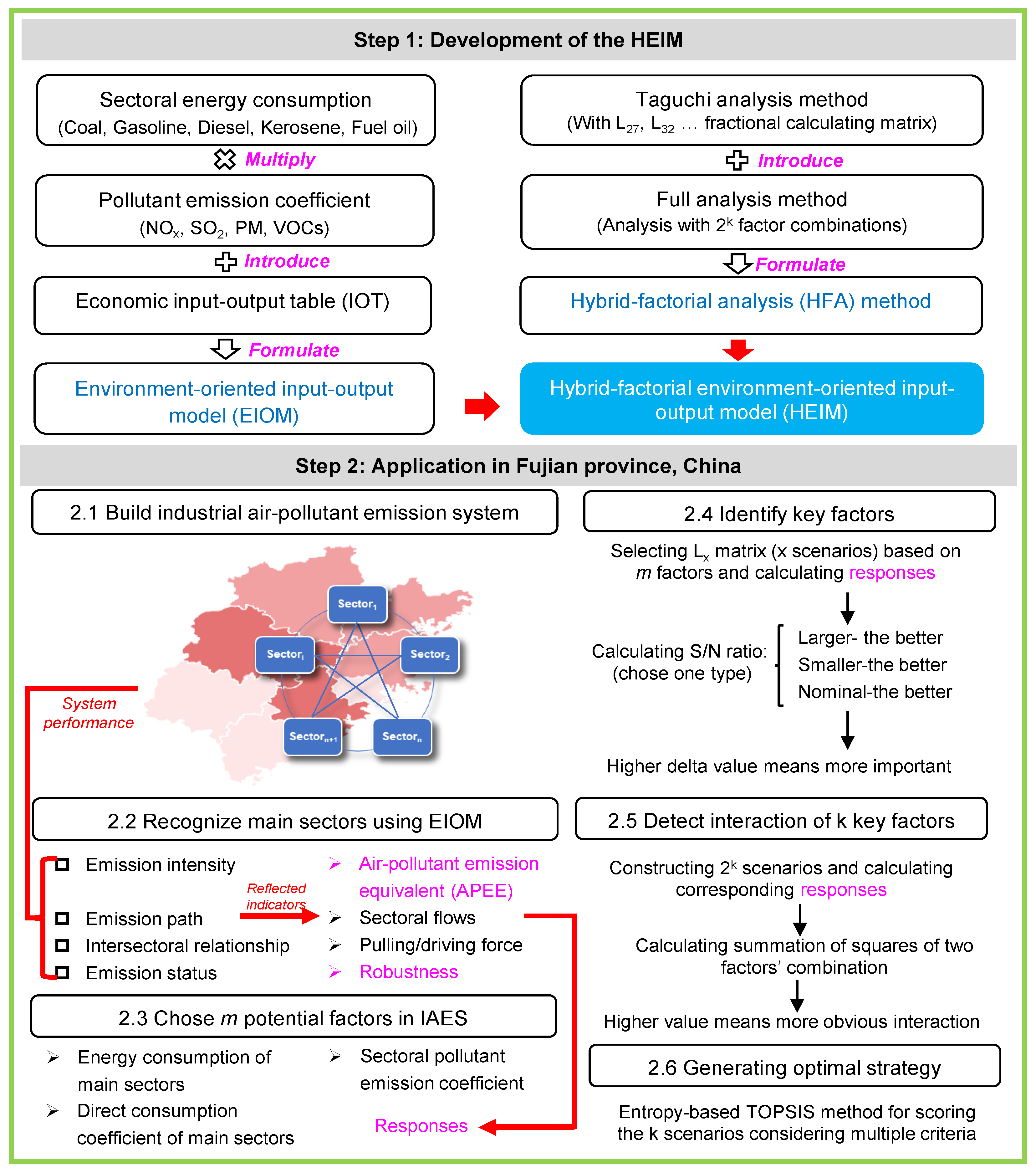
Figure 1. The framework of HEIM.
Sustainability 15 07717 g001
Figure 2. Air pollutants emitted from various sectors.
Sustainability 15 07717 g002
Figure 3. APEE flow among sectors.
Sustainability 15 07717 g003
Figure 4. Sectoral driving and pulling forces.
Sustainability 15 07717 g004
Figure 5. The relationship between efficiency and redundancy of IAES.
Sustainability 15 07717 g005
Figure 6. The amount and composition of APEE under Taguchi analysis.
Sustainability 15 07717 g006
Figure 7. System robustness under Taguchi analysis.
Sustainability 15 07717 g007
Figure 8. The main effects of designed factors on (a) APEE and (b) robustness.
Sustainability 15 07717 g008
Figure 9. The interactive effects of key factors on APEE (“*” means interaction).
Sustainability 15 07717 g009
Figure 10. The interactive effects of key factors on robustness (“*” means interaction).
Sustainability 15 07717 g010
Figure 11. The emissions of four air pollutants and robustness under full factorial analysis.
Sustainability 15 07717 g011
Figure 12. The four air pollutant reduction ratios, robustness improvement ratios and sectoral driving and pulling forces under selected scenarios.
Sustainability 15 07717 g012
Table 1. Abbreviations of 16 sectors.
No.SectorAbbreviation
1Agriculture, forestry, animal husbandry and fisheryAGR
2Mining industryMIN
3Food, drink, tea Manufacturing and tobacco processingFOO
4Textile productsTEX
5Timber processingTIM
6Paper productsPAP
7Petroleum processing, coking and nuclear fuel processingPET
8Chemical productsCHE
9Nonmetal minerals productsNON
10Metal processingMET
11Equipment manufacturingEQU
12Electricity production and supplyELE
13ConstructionCON
14Transportation, storage and postal servicesTRA
15Wholesale, retail and accommodationWHO
16Service industrySER
Table 2. Sectoral emission coefficients (unit: kg/ton).
Sector NOx SO2
CoalGasolineDieselKeroseneFuel OilCoalGasolineDieselKeroseneFuel Oil
AGR(3.30, 3.75)(9.70, 16.70)(4.00, 5.77)(3.58, 4.48)(3.10, 3.50)(3.80, 4.19)(0.02, 0.10)(0.70, 0.90)(1.00, 2.24)(8.00, 10.00)
MIN-EQU(3.30, 4.30)(3.27, 3.67)(3.21, 3.67)(3.27, 3.67)(3.20, 3.60)(3.20, 4.00)(0.02, 0.10)(0.70, 0.90)(1.00, 2.24)(8.00, 10.00)
ELE(1.70, 2.70)(3.27, 3.67)(3.21, 3.41)-(3.00, 3.41)(2.40, 3.20)(0.02, 0.10)(0.56, 0.70)-(6.00, 8.08)
CON(5.25, 7.25)(9.70, 16.70)(3.27, 9.62)--(7.66, 9.86)(0.02, 0.10)(0.70, 0.90)--
TRA(5.25, 7.50)(3.65, 9.36)(12.66, 14.25)(21.00, 27.40)(21.00, 27.40)(3.60, 4.19)(0.02, 0.10)(0.10, 0.10)(1.00, 2.24)(8.00, 10.00)
WHO, SER(2.00, 3.70)(9.70, 16.70)(3.21, 5.77)--(3.60, 4.19)(0.02, 0.10)(0.70, 0.90)--
Sector PM VOCs
CoalGasolineDieselKeroseneFuel OilCoalGasolineDieselKeroseneFuel Oil
AGR(3.30, 3.71)(1.30, 1.74)(1.30, 1.74)(0.60, 0.90)(1.30, 1.74)(0.45, 0.60)(3.00, 3.37)(3.00, 3.37)(0.13, 0.15)(3.00, 3.37)
MIN-EQU(2.00, 2.50)(0.10, 0.31)(0.40, 0.50)(0.60, 0.90)(0.45, 1.03)(0.18, 0.39)(0.07, 0.10)(0.12, 0.15)(0.13, 0.15)(0.15, 0.17)
ELE(1.30, 2.06)(0.10, 0.31)(0.40, 0.50)-(0.45, 0.85)(0.15, 0.18)(0.07, 0.10)(0.12, 0.13)-(0.12, 0.13)
CON(3.30, 3.50)(2.00, 2.09)(2.00, 2.09)--(0.18, 0.60)(3.00, 3.39)(3.00, 3.39)--
TRA(3.30, 3.50)(0.03, 0.04)(1.00, 1.10)(0.60, 0.90)(0.45, 1.03)(0.45, 0.60)(3.00, 3.14)(0.12, 0.15)(0.13, 0.15)(0.15, 0.17)
WHO, SER(3.30, 3.50)(0.13, 0.31)(0.40, 0.50)--(0.45, 0.60)(0.09, 0.10)(0.12, 0.15)--
Note: (number, number) correspond to (L level, H level).
Table 3. The abbreviations and descriptions of designed factors.
FactorsDescriptionLevel (L)Level (H)
ELE_coalConsumption of coal in ELE (106 ton)35.7744.71
NON_coalConsumption of coal in NON (106 ton)6.688.35
CHE_coalConsumption of coal in CHE (106 ton)4.665.83
MET_coalConsumption of coal in MET (106 ton)3.544.43
TRA_gasolineConsumption of gasoline in TRA (106 ton)1.732.16
TRA_dieselConsumption of diesel in TRA (106 ton)2.092.61
TRA_keroseneConsumption of kerosene in TRA (106 ton)1.051.31
TRA_fuel oilConsumption of fuel oil in TRA (106 ton)0.620.78
EQU_aDirect consumption coefficient of EQU0.370.46
TEX_aDirect consumption coefficient of TEX0.340.43
SER_aDirect consumption coefficient of SER0.200.25
CON_aDirect consumption coefficient of CON0.010.01
WHO_aDirect consumption coefficient of WHO0.020.02
NOxNOx emission from unit energy (kg/ton)**
SO2SO2 emission from unit energy (kg/ton)**
PM2.5PM2.5 emission from unit energy (kg/ton)**
VOCsVOCs emission from unit energy (kg/ton)**
Note: ‘*’ please refer to Table 2.
Table 4. S/N ratio response of designed factors to APEE (Smaller the better).
LevelELE_coalNON_coalCHE_coalMET_coalTRA_gasolineTRA_dieselTRA_keroseneTRA_fuel oilEQU_a
L−170.533−170.745−170.778−170.800−170.830−170.798−170.792−170.812−170.864
H−171.194−170.983−170.949−170.928−170.898−170.929−170.935−170.915−170.864
Delta0.6610.2380.1710.1280.0680.1310.1430.1030
Rank245811761017
LevelTEX_aSER_aCON_aWHO_aNOxSO2PMVOCs
L−170.863−170.865−170.865−170.866−170.396−170.633−170.807−170.835
H−170.865−170.863−170.863−170.862−171.332−171.095−170.921−170.892
Delta0.0020.0020.0030.0040.9360.4620.1140.057
Rank1516141313912
Table 5. S/N ratio response of designed factors to robustness (Larger the better).
LevelELE_coalNON_coalCHE_coalMET_coalTRA_gasolineTRA_dieselTRA_keroseneTRA_fuel oilEQU_a
L−9.352−9.427−9.472−9.340−9.344−9.342−9.340−9.352−9.003
H−9.335−9.261−9.215−9.348−9.343−9.346−9.347−9.336−9.684
Delta0.0170.1660.2570.0080.0010.0040.0070.0160.681
Rank7321017131181
LevelTEX_aSER_aCON_aWHO_aNOxSO2PMVOCs
L−9.373−9.377−9.341−9.336−9.335−9.342−9.343−9.343
H−9.315−9.311−9.346−9.351−9.352−9.345−9.344−9.344
Delta0.0580.0660.0050.0150.0170.0040.0010.002
Rank541296141615
Disclaimer/Publisher’s Note: The statements, opinions and data contained in all publications are solely those of the individual author(s) and contributor(s) and not of MDPI and/or the editor(s). MDPI and/or the editor(s) disclaim responsibility for any injury to people or property resulting from any ideas, methods, instructions or products referred to in the content.