Hyperspectral Classification of Hazardous Materials Based on Deep Learning

Abstract

The identification of hazardous materials is a key measure in the prevention and control of fire and explosion disasters. Conventional techniques used to identify hazardous materials include contact detection and post-sampling laboratory testing, which cannot meet the needs of extreme environments, where personnel and equipment are not accessible for on-site detection. To address this problem, this paper proposes a method for the classification and identification of hazardous materials based on convolutional neural networks, which can achieve non-contact remote detection of hazardous materials. Firstly, a dataset containing 1800 hyperspectral images of hazardous materials, which can be used for deep learning, is constructed based on the hazardous materials hyperspectral data cube. Secondly, based on this, an improved ResNet50-based classification method for hazardous materials is proposed, which innovatively utilizes a classification network based on offset sampling convolution and split context-gated convolution. The results show that the method can achieve 93.9% classification accuracy for hazardous materials, which is 1% better than the classification accuracy of the original ResNet50 network. The network also has high performance under small data volume conditions, effectively solving the problem of low classification accuracy due to small data volume and blurred image data features of labelled hazardous material images. In addition, it was found that offset sampling convolution and split context-gated convolution showed synergistic effects in improving the performance of the network.

1. Introduction

Several major explosion accidents have occurred in recent years, including the “8/4” massive explosion accident at the Beirut Port in Lebanon in 2020, the “3/21” massive explosion accident in Xiangshui, Jiangsu, China in 2019, and the “8/12” massive fire and explosion accident at the port of Tianjin, China in 2015. These accidents caused heavy casualties and property losses and seriously affected the economic and social development. Therefore, effective prevention and rational response to explosion accidents are of great importance. As a key measure for the prevention and control of explosion accidents and secondary disasters, the identification of hazardous materials can effectively reduce the risk of explosion accidents and improve our ability to deal with explosion accidents appropriately.

Common methods for the detection of hazardous materials include a variety of techniques such as gas chromatography, liquid chromatography, ion chromatography, mass spectrometry, differential scanning calorimetry (DSC), thermogravimetric analysis (TGA), spectrophotometry, X-ray spectroscopy, UV spectroscopy, Fourier transform infrared spectroscopy, Raman spectroscopy, and terahertz spectroscopy [1,2,3,4,5,6,7]. These methods are relatively mature technologies, and each has its own advantages and suitable objects for detection. However, they all have a common drawback, which is that they require contact detection or laboratory detection after sampling. This limits the timeliness of these approaches and they are not capable of remote non-contact detection and recognition.

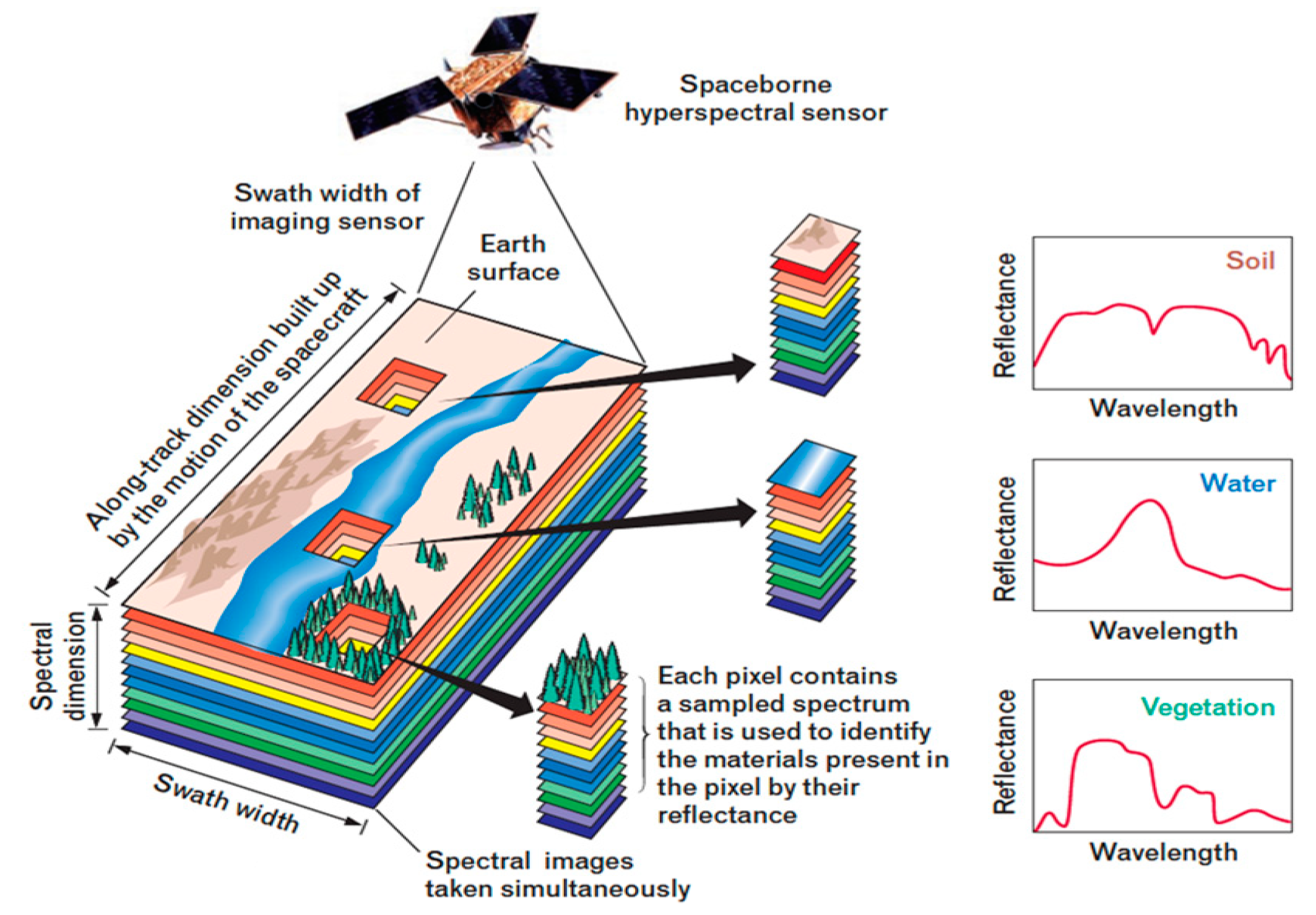
However, due to the urgent need for detection and recognition, as well as the complexity and the high risks associated with the disaster site environment, remote detection is typically used for the detection and recognition of hazardous materials in actual explosion accidents. Therefore, hyperspectral imaging technology, which is capable of non-contact remote detection, has attracted great attention. Hyperspectral imaging technology has the characteristics of both spectroscopy and imaging techniques and can achieve the detection of one-dimensional (1D) spectral information and two-dimensional (2D) spatial information [8], as shown in Figure 1 [9]. As a nondestructive remote sensing technology, hyperspectral imaging technology has been widely applied in aerospace [10], agriculture, forestry, animal husbandry [11], food safety [12], and medical diagnosis [13] due to its advantages, such as multi-band, high resolution, and spectral image fusion. After nearly 40 years of development, hyperspectral imaging technology has been widely studied and applied in a variety of interdisciplinary fields. With regard to the detection and identification of hazardous materials, Klueva, Oksana et al. [14] developed reagent-less, non-contact, non-destructive sensors for the real-time detection of hazardous materials based on widefield shortwave infrared (SWIR) and Raman hyperspectral imaging (HSI). They discussed the application of the SWIR-HSI and Raman sensing technologies to homeland security and law enforcement for standoff detection of homemade explosives and illicit drugs and their precursors at vehicle and personnel checkpoints. The application of sensors could eliminate and mitigate the escalating threat to civilian and military personnel posed by the proliferation of chemical and explosive threats and illicit drugs. Gwon, Yeonghwa et al. [15] obtained hyperspectral images of 18 types of hazardous chemicals using remote sensing techniques and the latest sensor technology, and investigated the feasibility of using hyperspectral images to individually classify 18 types of hazardous chemicals to overcome the limitations of contact detection technology in detecting the leakage of hazardous chemicals into aquatic systems for rapid detection and response in the event of chemical spills. Ruxton, Keith et al. [16] successfully detected and identified hazardous materials deposited on a range of surfaces using the negative contraction imager (NCI) by processing and analyzing the fundamental absorption bands of hazardous materials in the mid-wave infrared band. By using spectral fitting algorithms to aid agent identification, a hyperspectral imaging-based method of long-range detection was provided to keep operators and equipment away from potentially lethal threat agents. Fischbach, T et al. [17] proposed a method based on laser-induced fluorescence that uses a lot information (time-dependent spectral data and local information) and predicts hazardous materials by statistical data analysis. The method allows for a direct classification of the detected materials and takes into account changes in material parameters (physical state and concentration). Nelson, MP et al. [18] developed an HSI Aperio sensor for real-time wide-area surveillance and standoff detection of explosives, chemical threats, and narcotics for both government and commercial use. Unlike existing detection technologies, which often require close proximity for detection, putting operators and expensive equipment at risk, the handheld sensor has faster data acquisition, faster image processing, and increased detection capability compared to previous sensors. In addition, the ease of use of handheld detectors allows the individual operator to detect threats from a safe distance, improving the effectiveness of locating and identifying threats while reducing the risk to the individual.

Recently, deep-learning-based hyperspectral image recognition and classification has become a commonly researched topic. As a typical deep learning algorithm, the convolutional neural network (CNN) has been widely applied in target detection, image classification, and semantic segmentation. In fact, CNNs are currently the most widely used network model for hyperspectral image classification. CNN-based hyperspectral image classification methods mainly include classification methods based on spatial features, spectral features, and joint spatial–spectral features.

Liang et al. [19] proposed a hyperspectral image classification method based on the deep learning features and sparse representation based on the spatial features of a hyperspectral image. This method used a sparse representation classification framework to extract deep features from image data. Experimental results showed that this method exploited the intrinsic low-dimensional structure of deep features and exhibited improved classification performance compared with widely used feature search algorithms such as extended multi-attribute profiles (EMAPs) and sparse coding (SC). Hu et al. [20] investigated hyperspectral image classification using a 1D-CNN network with one convolutional layer, one pooling layer, and two fully connected layers, based on the spectral features of hyperspectral images. Experimental results demonstrated that this method showed better classification performance than conventional support vector machine methods. Based on the joint spatial–spectral features of hyperspectral images, Yue et al. [21] proposed a deep learning framework that can be used for hyperspectral image classification, which was the first to introduce deep convolutional neural networks (DCNNs) for hierarchical deep feature extraction in the field of hyperspectral image classification. First, a feature map generation algorithm was proposed to generate spectral and spatial feature maps. Then, the DCNNs-LR (deep convolutional neural networks and logistic regression) classifier was trained to obtain useful advanced features and to fine-tune the overall model. Comparative experiments on widely used hyperspectral datasets showed that the DCNNs-LR classifier constructed in this deep learning framework exhibited improved classification accuracy compared to that of conventional classifiers. Hua, D et al. [22] experimented with Keras to create a convolutional neural network and with OpenCV to create a real-time video that distinguishes hazardous waste from other recyclable materials. By using machine learning, the model was able to categorize different recyclable materials with around 90% accuracy, protecting more people from negative effects. Seo, M and Lee, SW [23] generated a database of hazardous compounds using data provided by the Ministry of the Environment, and trained and learned the characterized dataset using a convolutional neural-network-based algorithm, resulting in a CNN-based model with up to 90% accuracy. The model can effectively distinguish hazardous chemicals without any additional testing and can replace traditional methods of predicting chemical toxicity. Liu, DM et al. [24] proposed a lightweight hazardous liquid detection method based on the depthwise separable convolution for X-ray security screening. Firstly, a dataset of seven common hazardous liquids with multiple postures in two detection environments was established. Secondly, a novel detection framework was proposed using the dual-energy X-ray data, instead of pseudocolor images, as the objects to be detected, which improves the detection accuracy and realizes the parallel operation of detection and imaging. Thirdly, based on the depthwise separable convolution and the squeeze-and-excitation block, a lightweight object location network and a lightweight hazardous liquid classification network were designed as the backbone networks of the method to achieve the location and classification of the hazardous liquids, respectively. Compared to the existing methods, the experimental results demonstrate that the method has better performance and wider applicability.

In summary, deep learning algorithms represented by CNNs have achieved remarkable results in hyperspectral image classification, not only effectively compensating for the drawbacks of conventional classification methods, but also improving the accuracy of hyperspectral image classification. However, the classification of hyperspectral spectra of typical hazardous materials still requires further investigation. Here, we investigated deep-learning-based recognition and classification of typical hazardous material spectra with the aim of improving the applicability and accuracy of deep learning in the recognition and classification of typical hazardous material spectra. In addition, a novel method for the long-distance and non-contact detection and recognition of hazardous materials was provided. A theoretical basis has been established and experimental results have been produced, which will be of great use in the detection and early warning of hazardous materials, as well as expanding the applications of hyperspectral imaging technology and computer vision technology.

2. Related Work

CNNs are deep learning models that can learn features automatically and have been used with great success in areas such as image classification and target detection. In hyperspectral image classification, CNNs are able to handle two-dimensional and even three-dimensional data, making them a common network for hyperspectral image classification tasks. In addition, the combination of attention mechanism, migration learning, and hybrid network strategies is well suited to compensate for the high-dimensional nature of hyperspectral data, the scarcity of training samples, the non-linearity of the data, and to better improve the classification results. The application of CNNs in hyperspectral image classification is mainly divided into several aspects, such as feature extraction, classification, target detection, and data enhancement. Firstly, CNNs can automatically learn features in hyperspectral images to obtain a more robust feature representation that can be used in subsequent classification tasks. Secondly, CNNs can classify different objects or scenes in hyperspectral images. Additionally, CNNs can detect different objects or scenes in a hyperspectral image. Finally, CNNs can increase the diversity of the training data through data augmentation, which improves the generalization ability of the model, for example, by rotating, mirroring, and scaling. In conclusion, the application of CNNs to hyperspectral image classification has great potential to contribute to a better understanding of the information in hyperspectral images and to support subsequent applications.

In recent years, with the application of CNNs to image classification, several high-performance image classification networks have emerged, including ResNet [25], MobileNet [26], and DenseNet [27]. In contrast, ResNet and its improved networks show good performance in most tasks. ResNet was an important milestone in the development of CNNs, as its introduction solved the problem of network degradation by increasing the network depth of CNNs. To address this problem, a residual block was proposed for ResNet. Experiments on the ResNet network showed that when the residual block was used, the network depth could be increased to more than 1000 layers while maintaining some network performance.

In 2015, ResNet used skip connections to effectively address the problem of gradient disappearance in the deep network training process, and many researchers have since proposed improved mechanisms based on ResNet. Many methods aimed to improve the feature extraction capabilities of the network, such as the attention mechanism of SENet [28]. Some methods aimed to reduce the model complexity while maintaining its performance, such as the grouping convolution of ResNeXt [29]. Other methods enhanced network performance by improving the network structure for tasks, such as the image segmentation operation of progressive multi-granularity training [30]. In short, the ResNet and its improved networks have certain advantages over most networks in terms of network complexity and network performance. In this paper, we also improve on the ResNet network, and then obtained a more effective hyperspectral spectra classification network for hazardous materials.

2.1. Offset Sampling Convolution

The conventional convolution operation can be divided into the following two steps: (1) Performing sampling using a regular filter over the input feature map $x$; (2) Performing a weighted operation. $R$ defines the size of the convolution kernel. $P_n$ denotes all the pixels in the range of $R$, and $w$ denotes the convolution weighting factor. Each pixel $P_0$ on the output feature map $y$can be expressed by Equation (1), as follows:

$$y\left(P_0\right)={\displaystyle \sum }_{P_n\in R}w\left(P_n\right)\times x\left(P_0+P_n\right)$$

(1)

The deformable convolution adds an offset $△P_n$ to the conventional convolution, and $P_0$ can be expressed as

$$y\left(P_0\right)={\displaystyle \sum }_{P_n\in R}w\left(P_n\right)\times x\left(P_0+P_n+△P_n\right)$$

(2)

In this way, sampling becomes irregular and, because the learned $△P_n$ offset variable is generally fractional, the sampled pixel values are calculated by bilinear interpolation as

$$x\left(p\right)={\displaystyle \sum }_{q}G\left(q,p\right)\times x\left(q\right)$$

(3)

where $p$ denotes the offset fractional position, $q$ enumerates the feature map integer space position, and $G$ is the bilinear interpolation kernel.

The convolution of the conventional convolution kernel is a fixed-scale (generally, 3 × 3, 5 × 5) local operation, whereas the hyperspectral spectra of typical hazardous materials are curvilinear, and most of the area is background area with ineffective information. The features obtained from a regular sampling box cannot accurately reflect the curve features of hyperspectral spectra. Therefore, an offset sampling convention block was introduced to increase the ability to learn horizontal and vertical offsets when the conventional convolution learns and extracts features, thus achieving a more effective extraction of the curve features of the typical hyperspectral spectra of hazardous materials.

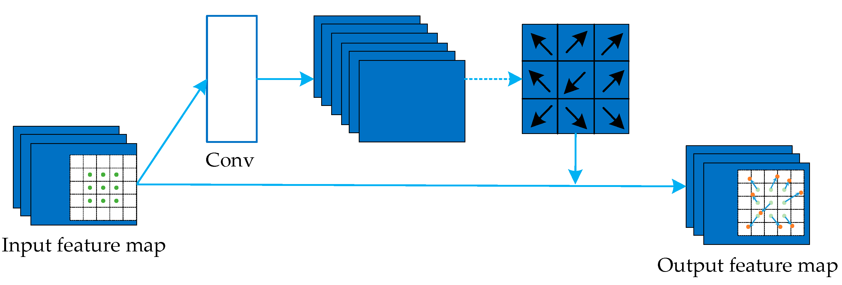
Dai et al. [31] proposed the offset sampling convolution (DConv, see Figure 2) and demonstrated that the offset sampling convolution operation has a better modelling capability for deformed objects compared to other approaches. Meanwhile, the offset sampling position was better adapted to the shape and size of the object itself, which improved the network performance. In this study, the offset sampling block learned the horizontal and vertical displacement of each pixel in the original feature map through a convolutional layer. It then calculated the offset pixel value based on this displacement by bilinear interpolation to generate a new feature map as the input of the next layer, and the sampled pixel position was transformed from the green dots shown in Figure 2 to the orange dots seen after the offset.

2.2. Attention Model

In recent years, the combination of CNNs and the attention mechanism have become important in the study of CNNs. The attention mechanism enhances the data significance learning ability of a network and provides an interpretation for CNN feature extraction. The attention mechanism of CNNs can be divided into three categories: channel-domain attention, spatial-domain attention, and mixed-domain attention. Depending on the attention mechanism, CNNs focus on different aspects.

Channel-domain attention measures the importance of channels by adding an attention mechanism to the channels and assigning different weights to different channels. Channels tend to learn different feature representations, and the network can perform better at distinguishing different features and learning key features by applying channel attention. Typical channel attention networks, such as SENet, add a branch to learn explicit connections between channels. The branch is designed with a global pooling layer to obtain global information, and passes through two fully connected layers to output the channel weight matrix.

Spatial-domain attention measures the importance of regions in a space by adding an attention mechanism to the space and assigning different weights to different pixels in the space. Regions in the space tend to learn the representativeness of each region in terms of features, and the network can perform better at distinguishing different regional features, learning key regions of the features and building connections among the key regions by applying spatial attention. Typical spatial attention mechanisms, such as non-local ones, can generate three sets of feature maps through three sets of 1 × 1 convolutions. They compress and reduce the dimension of the three sets of feature maps and then multiply two of their matrices to obtain the spatial attention matrix. Finally, they multiply it with another set to obtain the feature map of spatial attention.

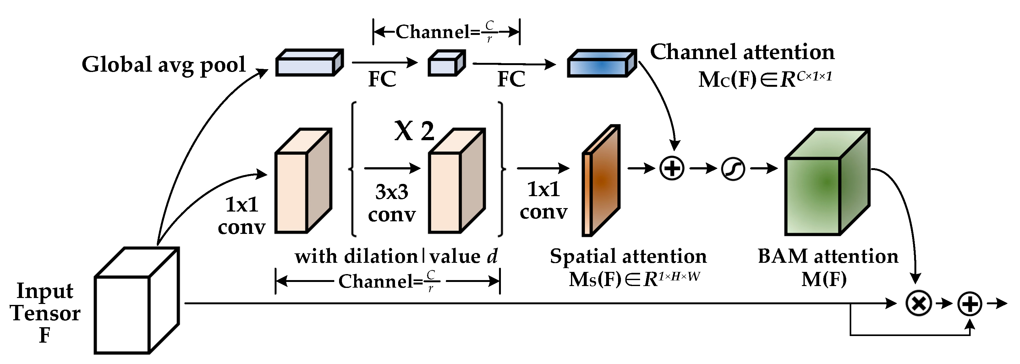
Mixed-domain attention is built by adding an attention mechanism in multiple dimensions, which can result in more focused network attention. Typical mixed-domain attention mechanisms include CBAM [32] (Figure 3) and BAM [33] (Figure 4). In CBAM, the channel attention block is sequentially related to the spatial attention block. The feature map is first multiplied by the channel attention matrix to obtain channel attention, and then multiplied by the spatial attention matrix to obtain spatial attention. For BAM, the spatial attention block is connected in parallel with the channel attention block, and then the attention matrices of the two blocks are expanded to the same size and are multiplied element by element. A comparison of the two networks shows that each of the two mixed-domain attention mechanisms can improve the accuracy of target detection or object classification but CBAM performs better than BAM. A possible reason for this is that the spatial attention matrix in CBAM is generated according to the feature map with channel attention, which is more accurate than the spatial attention in BAM.

2.3. Split CGC

Neurons in the human brain change their function according to the environment and the task. To mimic this function, a spatial context mechanism has been introduced into the modelling process of deep neural network models. Specifically, the convolution kernel in a CNN has the property of a local receptive field. In deep CNNs, the convolution kernels of the deeper convolution layers gradually increase the receptive field as feature abstraction is performed by stacking the convolution layers layer by layer. Conventional convolution is essentially an aggregation of local information and cannot model the relationship (spatial context) between any pixels in the hyperspectral spectra of typical hazardous materials. Since the shape of the curve is the most important feature in the hyperspectral spectra of typical hazardous materials, there is little correlation between the curve and the off-curve pixels. Additionally, only the global features of the hyperspectral spectra can accurately represent their semantic information, while the local features of the hyperspectral spectra may interfere with model recognition. Therefore, the overall recognition network needs to pay more attention to the effective pixels and reduce the interference of irrelevant features.

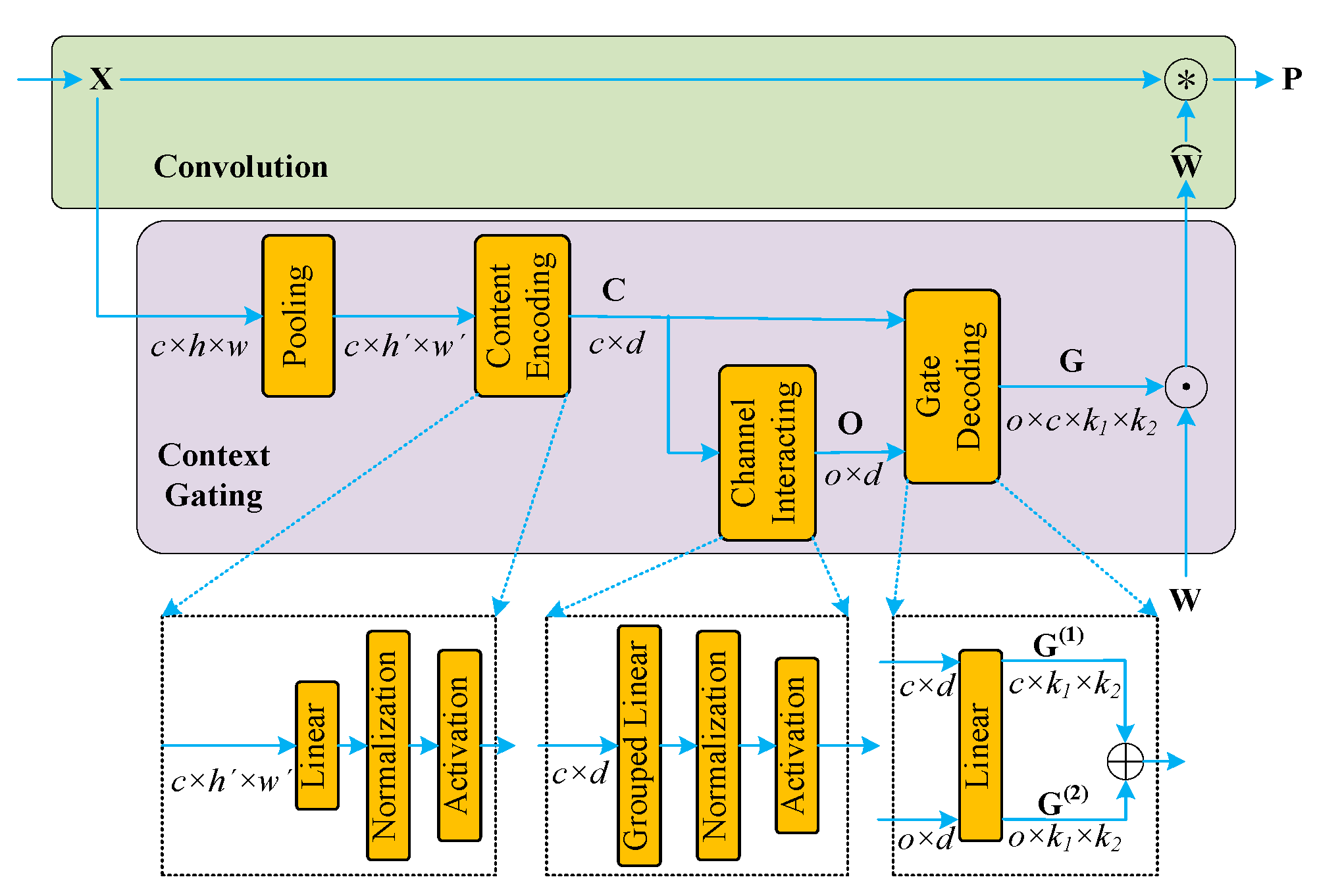
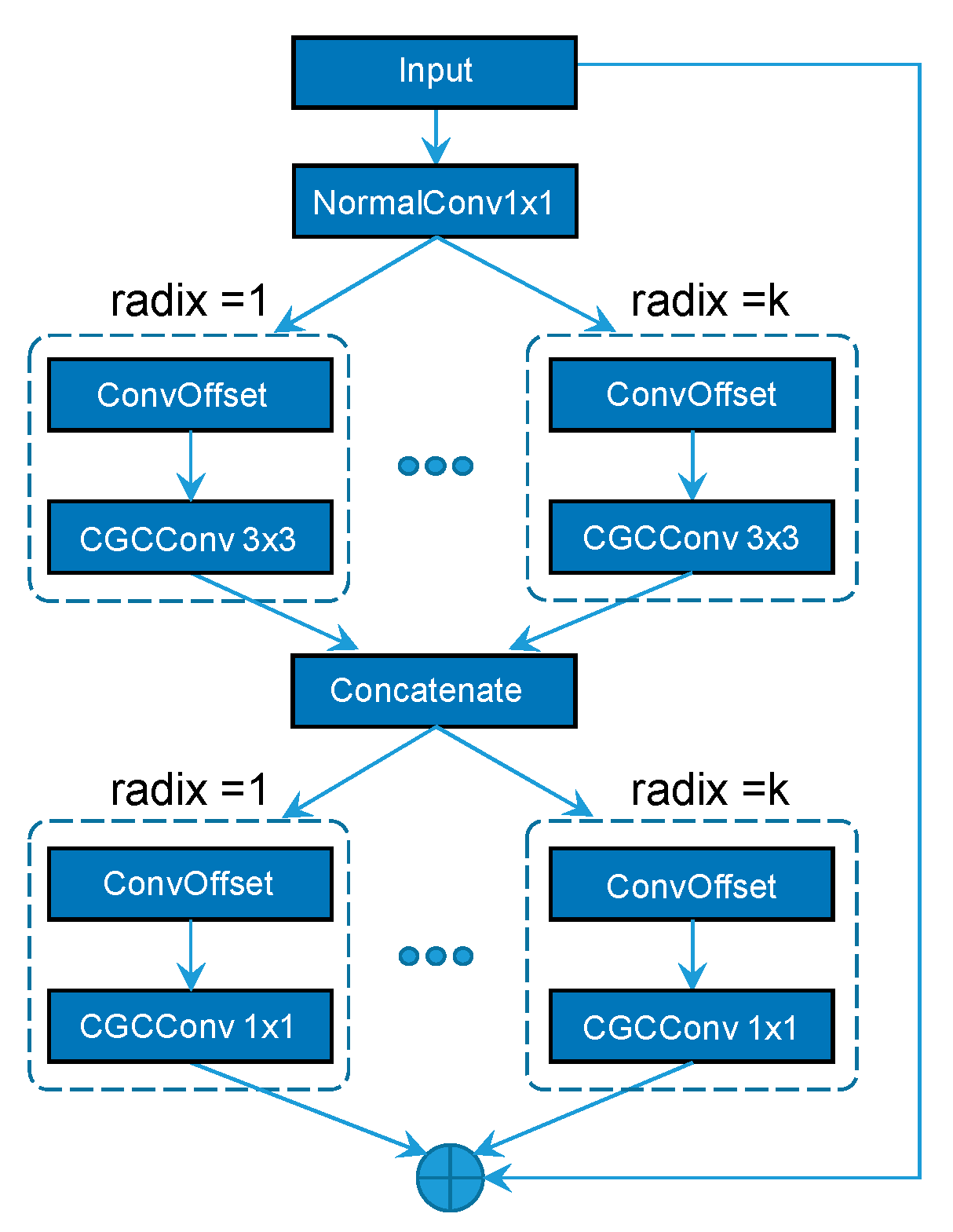
Inspired by context-gated convolution (CGC) (Figure 5) [34], we used a global feature interaction method to integrate the global context into the local feature representation through an attention mechanism and to modulate the intermediate feature mapping. This enabled the small convolution kernel to learn global features, establish explicit connections with the curves on the hyperspectral spectra, and eliminate the interference from irrelevant pixels. Based on the offset sampling residual network mentioned above, we introduced Split CGC, which used contextual information to modulate the convolution kernel weights through multi-level attention. This enabled the extraction of features with better determination and differentiating capabilities for different types of hyperspectral spectra of typical hazardous materials. The original CGC block transformed the convolutional layer into an “adaptive processor” that could autonomously adjust the weight parameters of the convolution kernel according to the semantic information of the image, similar to the spatial attention mechanism, and assign different weights to different spatial positions in the image. Studies involving BAM and CBAM have verified that the mixed-domain attention mechanism combining the space-domain attention mechanism and the channel-domain attention mechanism can further improve the feature extraction capability of a model. Therefore, based on the original CGC block, we proposed the Split CGC block, as shown in Figure 6, which introduced the channel attention mechanism based on the spatial attention mechanism of the original CGC block, forming a mixed-domain attention mechanism, thus enabling the recognition network to more effectively extract the hyperspectral spectra features of different types of typical hazardous materials.

An improved SplitCGC module based on ResNet allows the grouping of input feature maps in the channel dimension. The number of groups can be controlled by hyperparameters radix. Weights are then assigned to each group of convolutional kernels after grouping by CGC, which is equivalent to assigning different weights to different spatial locations of the feature map. CGC can efficiently generate gates of convolutional kernels so that the weights can be modified according to the global context. Moreover, CGC can better capture local patterns, synthesize discriminative features, and continuously improve the generalizability of traditional convolution with negligible increase in complexity for a variety of tasks, including image classification, action recognition, and machine translation. As shown in Figure 5, the CGC consists of three components, namely the context encoding module, the channel interaction module, and the gate decoding module. First, a pooling layer is used to reduce the spatial resolution to h′ × w′ and the resized feature mapping is provided to the context encoding module. The context encoding module encodes information from all spatial locations of each channel and extracts a feature representation of the global context. The resized feature maps in each channel are then projected via a linear layer onto the feature vector d. Secondly, the feature representations are projected into the space of output dimension o via channel interactions. Finally, gate decoding generates G⁽¹⁾ and G⁽²⁾ from the feature representation C and the projection representation O, and constructs the gate G via spatial interactions. The weights of the convolutional layers are then adjusted by element-by-element multiplication to merge the rich contextual information.

3. Materials and Methods

3.1. Dataset

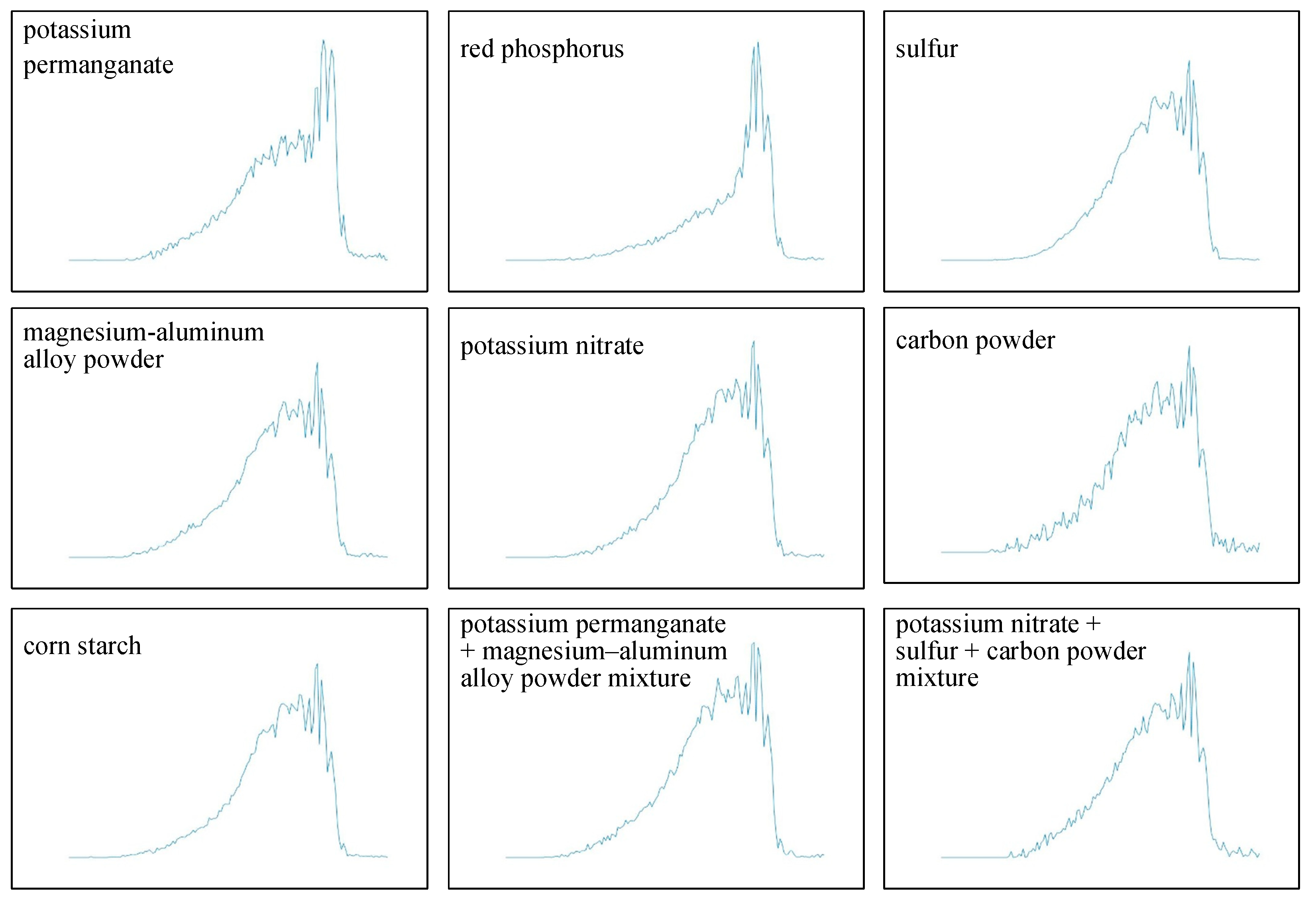
The hyperspectral spectra data of nine types of hazardous materials were used as the experimental dataset. The spectrum collection process is shown in Figure 7. A self-developed imaging spectrometer (self-developed equipment; Aerospace Information Research Institute, Chinese Academy of Sciences; Dyson optical structure; Fery prism as a light splitting element; spectral range 400–1000 nm; 240 bands; instantaneous angular resolution 0.5 mrad; field of view 30°; frame rate 50 fps) was used to collect the spectra data of the hazardous materials. The hazardous material targets were placed horizontally, adjacent to the ground, in front of the laboratory, and the visible light imaging spectrometer was placed on the floor of the fourth floor of the laboratory (the distance between the instrument and the hazardous material target is approximately 30 m). The standard reflector and the hazardous material targets were placed in the same area to ensure that both appeared in the push-broom field of view at the same time. Push-broom imaging was achieved by controlling the rotation of the turntable. The above steps were repeated 3 times to obtain 3 hyperspectral data cubes of hazardous materials. The obtained hyperspectral data cubes were radiometrically corrected, atmospherically corrected, and geometrically corrected to remove the influence of background factors, such as sampling distance and light, on the hyperspectral images. Based on the corrected hyperspectral data cubes, the reflectivity–wavelength spectrum curves of the hazardous materials can be obtained. To eliminate the influence of the coordinate axes on the recognition and classification of the hazardous materials, the axes were removed from the images, as shown in Figure 8. The nine types of hazardous materials were potassium permanganate, red phosphorus, sulfur, magnesium–aluminum alloy powder, potassium nitrate, carbon powder, corn starch, a potassium permanganate + magnesium–aluminum alloy powder mixture, and a potassium nitrate + sulfur + carbon powder mixture in our study to cover the basic different common types of solid hazardous materials, including flammables, strong oxidizers, metal powders, and non-metal powders. The volume of each component of the mixtures is the same. See

Table 1. Physical properties of the hazardous materials.

No.	Sample	Density (g·cm−3)	Color	Purity
1	Potassium permanganate	2.70	Black purple	AR
2	Red phosphorus	2.34	Reddish-brown	AR
3	Sulfur	2.07	Yellow	CP
4	Magnesium–aluminum alloy powder	2.66	Silver gray	CP
5	Potassium nitrate	2.11	White	AR
6	Carbon powder	0.45	Black	AR
7	Corn starch	0.55	Pale yellow	LR

for the physical properties of the seven single hazardous materials, including density, color, and purity. The dataset was constructed by the authors based on the hyperspectral remote sensing data cube of nine types of hazardous materials, with a total of 1800 images (200 images for each type). From this dataset, 70% (1260) of the images were randomly selected as the training set and 30% (540 images) as the test set.

3.2. Experimental Design

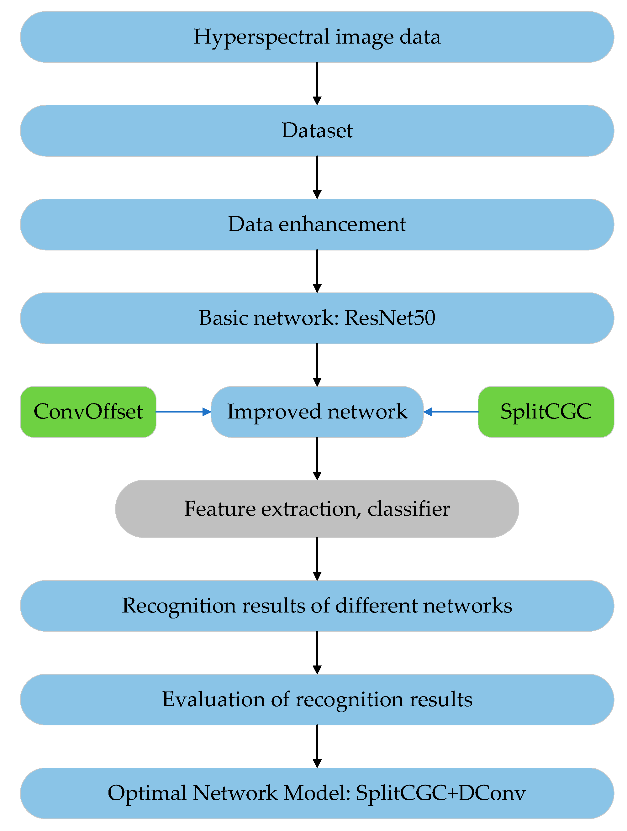
Figure 9 illustrates the experimental procedure. Firstly, the hyperspectral spectra data of typical hazardous materials were obtained from the hyperspectral data cube to form a hyperspectral dataset, and secondly, the hyperspectral spectra data of typical hazardous materials were enhanced. As the hyperspectral spectra are not rotationally invariant and have obvious background contrast, the experiment did not include geometric and color transformations. Additionally, because only full hyperspectral spectra can accurately represent image information, methods that could result in loss of image information, such as cropping, were not used in the experiment. Therefore, only size was adjusted to enhance the image data, and the hyperspectral spectra were uniformly reduced from 875 × 656 pixels to 100 × 100 pixels. The experiments showed that after data enhancement, the image information was preserved and the network computation consumption was reduced. Then, based on the ResNet50 network, the attention mechanism was introduced from the perspective of improving the feature extraction ability of the network. The experimental results obtained when attention was applied in different dimensions were compared and validated, with the network accuracy as the primary criterion and the network complexity as the secondary criterion. After the preliminary experiments, the CGC with the optimized results was improved, with the main direction of improvement being to further improve the feature extraction ability of the network. CGC is a CNN that learns features from data directly through the network. Therefore, in the experiments, the network was designed in the directions of data sampling and the multi-level attention superposition of the CNN, and these two improvement directions were compared and verified in terms of relevance. In this study, four sets of comparison experiments were designed, and the networks used in the four comparison experiments were CGC, CGC + DConv, Split CGC, and Split CGC + DConv. The purpose of this design was to compare and investigate the effects of adding Split CGC, DConv, and mixed-domain attention models on network performance. Additionally, this study also compared the recognition accuracies of the improved network with other spatial attention, channel attention, and mixed attention networks, and finally, the network was evaluated based on the recognition results of the nine types of typical hazardous materials, and the advantages of the improved network over the conventional network were verified.

3.3. Network Model Construction

The deep network used in this study was required to be able to train a network model with the highest classification accuracy in the existing hyperspectral spectra dataset of hazardous materials. Based on the presentation of related work, the ResNet network was used as the basic network model in this study. Depending on the different numbers of blocks, the ResNet network was divided into ResNet18, ResNet50, and ResNet101. Through a preliminary experimental comparison, the ResNet50 network was selected as the benchmark network for feature extraction and classification and was then improved in the subsequent experiments to obtain an improved network with higher classification accuracy than the benchmark network.

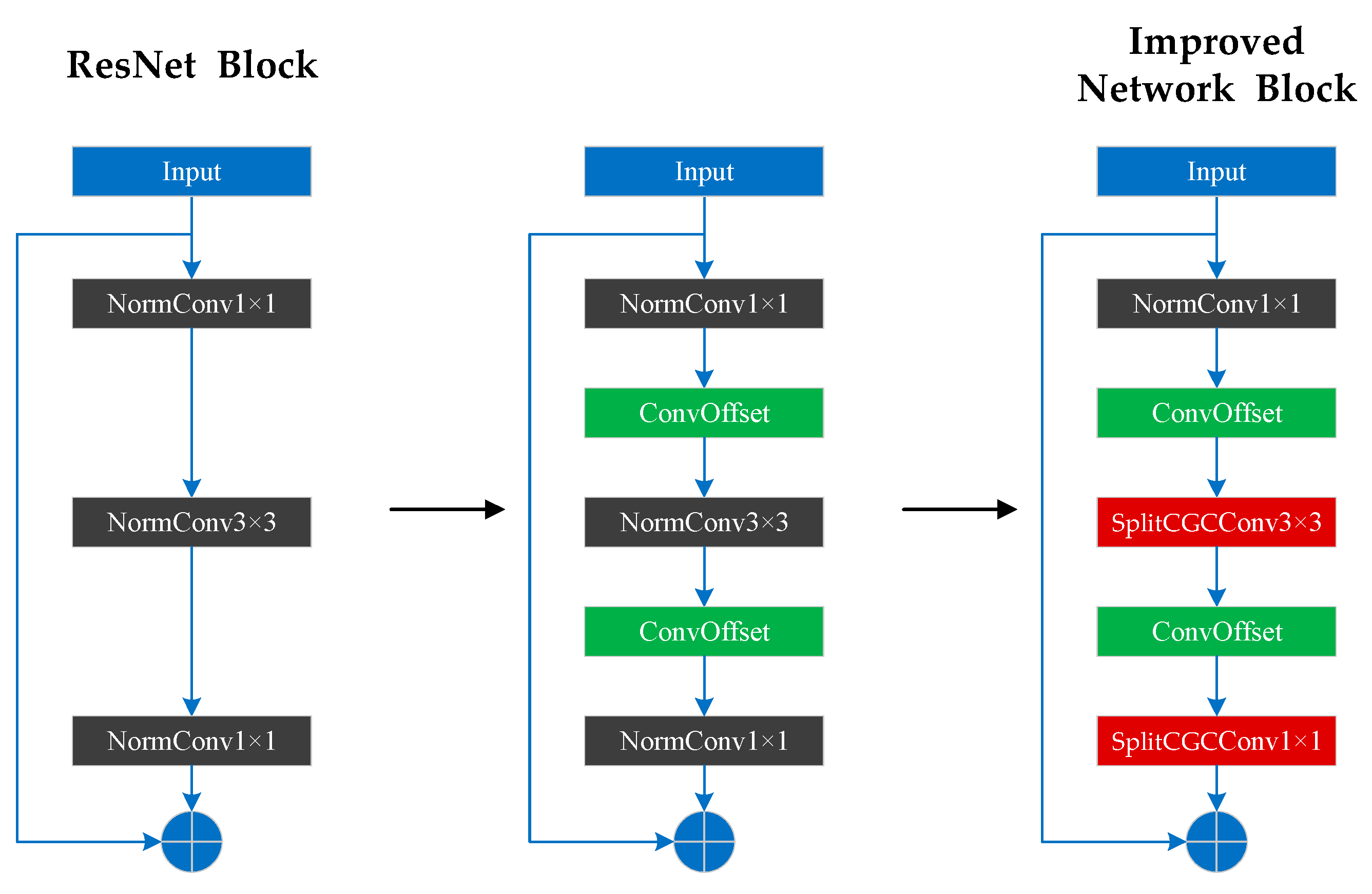
The hyperspectral spectra of hazardous materials are a curve of wavelength and reflectance, and the shape of the curve is the only effective feature available for the classification of the hyperspectral spectra of hazardous materials, which leads to two difficulties when compared with conventional image dataset classification. One is that it is difficult to achieve effective curve sampling using a conventional rectangular sampling box and the other is that the background area in a hyperspectral curve is large, making the effective key curve features weak and difficult to extract. To solve these problems, we proposed an offset sampling convention block and a SplitCGC block, and improved on the ResNet50 network: first, the offset sampling block was added in front of the 3 × 3 convolution and the second 1 × 1 convolution in each basic block of the ResNet50 network; finally, the 3 × 3 convolution and the second 1 × 1 convolution in each block of the ResNet50 network were changed to the SplitCGC convolution block. Figure 10 shows the improvement process of the improved network and the comparison with the ResNet block, where ConvOffset is the offset sampling convolution block and CGCConv is the CGC block.

3.4. Network Parameter Setting

Four sets of comparison experiments were designed with the same hyperparameters and learning rate update strategy, a batch size of 8, a learning rate of 2.5 × 10⁻⁴, a learning rate update strategy of turning to one third of the original learning rate every 20 epochs, a training epoch of 120 epochs, a loss function of cross-entropy function, a stochastic gradient descent (SGD) optimizer, a momentum of 0.9, and a weight decay of 5 × 10⁻⁴.

The loss function in CNNs includes the mean cross-entropy function, the sum-of-squares function, and the L1 function. In CNNs, the difference between a model and the objective model is represented by the loss value; the model is then corrected by back-propagating the loss value. Therefore, the selection of the loss function in CNNs is of great significance. The cross-entropy function was selected because the spectral recognition of typical hazardous materials is essentially a classification problem. The Softmax function is usually used to calculate the probability of each category, but when the Softmax function and other loss functions are used for calculation, the loss curve fluctuates, there is a large number of local extremes, and the training of the network is a non-convex optimization problem. In contrast, when the cross-entropy function is used, the loss curve is convex, and the training of the network is a convex optimization problem. When SGD is used for computation, the convex optimization problem shows better convergence. Additionally, compared to other loss functions, the cross-entropy function can better describe the gap between the model and the objective model in the classification problem.

The selection of optimizers plays a critical role in deep learning training and determines whether fast convergence and a high accuracy and recall rate can be achieved. Common optimizers include gradient-based optimizers (e.g., SGD and ASGD) and adaptive optimizers (e.g., Adagrad [35] and Adam [36]). SGD performs gradient descent for each sample in each batch of data, which causes SGD to iterate rapidly and in an uncertain direction as the gradient is updated. Compared with other adaptive optimizers, SGD has both advantages and disadvantages as a result of this feature. The advantage is that the fast random update direction of SGD can help the network to discard local extrema, so that the network can be trained more completely, which cannot be achieved by adaptive optimizers. The disadvantage is that at low learning rates, the random stochastic gradient direction can cause the network to become trapped in a saddle point during updating, while at high learning rates, the network may miss the minima or oscillate around them. In addition, gradient descent is slower than adaptive optimizers due to the unstable update direction.

Considering that the main goal of the recognition of typical hazardous materials is to achieve higher recognition accuracy, an SGD optimizer is used in this experiment. Meanwhile, a learning rate update strategy, momentum, and weight decay are introduced to reduce the negative effects of SGD. The momentum is set to 0.9. Through the momentum update, the parameter vector increases its speed in the direction of the continuous gradient, which attenuates the oscillation of the loss value caused by the random update of the SGD, and thus speeding up the training.

In this study, the learning rate update strategy is gradient descent, and the learning rate changes to one third of the original rate in every 20 epochs. As mentioned above, the learning rate determines the magnitude of the network update; for the random update of SGD, an appropriate learning rate must be selected during the training process to achieve good results. The learning rate update strategy of the gradient descent results in the learning rate decay as the network is trained. In the early stages of training, SGD uses a high learning rate to make the network converge quickly to a local minimum, while in the later stages of training, SGD uses a low learning rate to make the network search around the local minimum to find the global minimum and thus obtain the optimized network model.

Due to the strict control of hazardous materials, it is difficult to obtain such samples to collect the data used in this experiment. Therefore, the experimental dataset is relatively small, resulting in the frequent occurrence of overfitting during the network training process; that is, the accuracy of the model training set is much higher than that of the test set. To overcome this problem, a weight decay factor is introduced to regularize the network, which can reduce the fluctuation caused by weights that are too large when the network is overfitted.

4. Results and Discussion

The experimental results of this study can be divided into two parts, namely the results from the comparison experiment of neural network optimizers and the results from the comparison experiment of the improved Split CGC + DConv network and other attention networks, such as the ResNet50 network.

4.1. Selection of a Neural Network Optimizer

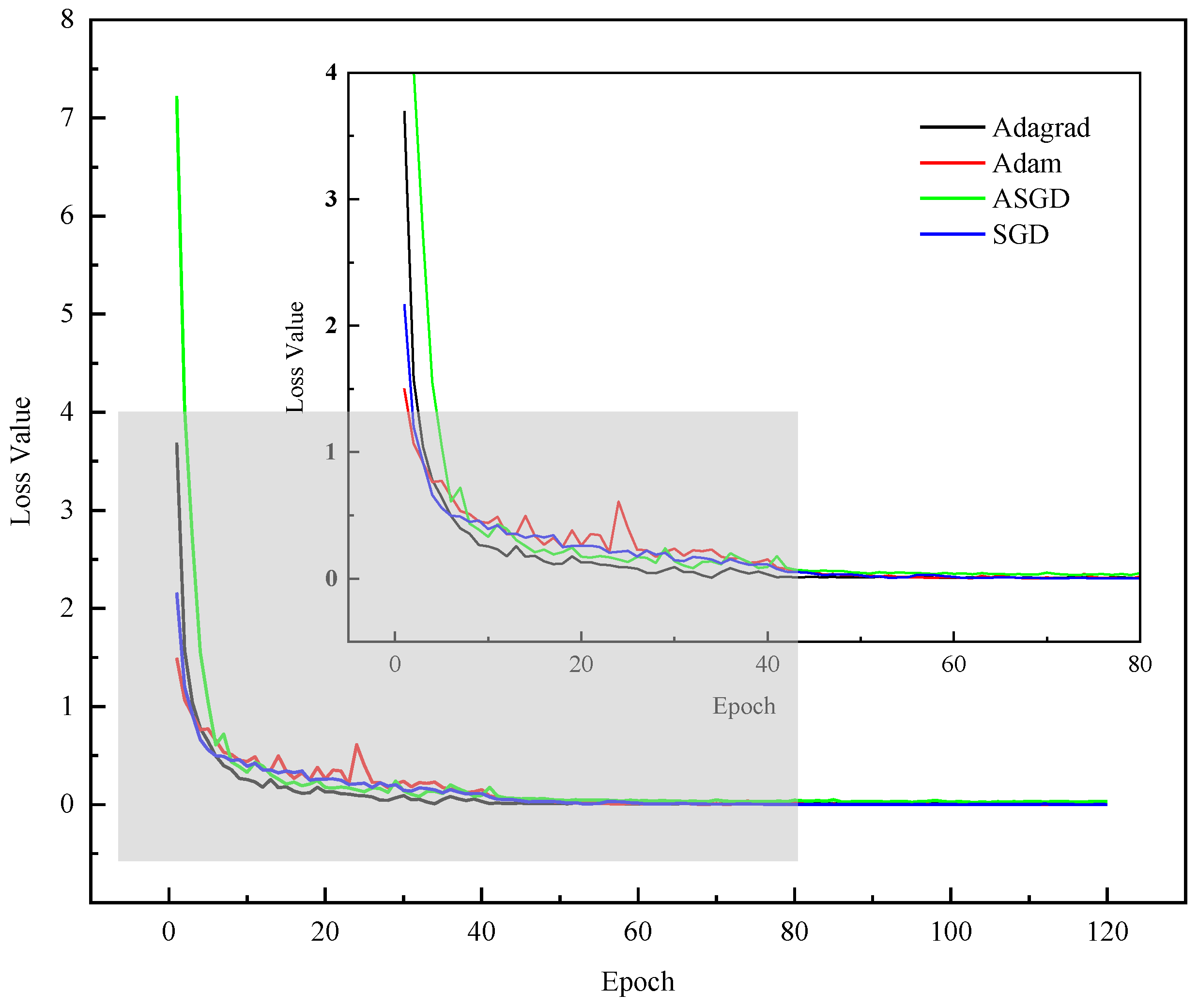
In this study, the effects of SGD optimizers with momentum and several common optimizers on network training were compared and studied in the Split CGC + Dconv network. SGD optimizers were then selected to train the network model. The experimental results are shown in Figure 11. A total of 120 training epochs were performed. To visualize the network training process, the average of the loss values (values of the loss function) calculated from all data batches in each epoch was taken as the loss value for that training epoch. According to Figure 11, the loss value of the network trained by the four optimizers decreased continuously from 0 to 60 epochs. In this case, there was a large gap between the network and the objective model, and the network had not yet fallen into the local minima. From 60 to 120 epochs, the loss value remained stable and the network reached the local minima and essentially converged. By comparing the gradient-based optimizers SGD and ASGD and the adaptive optimizers Adam and Adagrad, we found that the adaptive optimizers had some jitter and an unstable optimization direction at the beginning of the network training. Although the network converged later in training, it fell into local minima and showed almost no training effects after 70 epochs. The gradient-based optimizers adapted more slowly to the training process and showed convergence until the later stage of training. However, the perturbation caused by the random gradient of SGD meant that the network training did not stagnate at the local minima, but continued to explore around the local minima, allowing the SGD optimizer to converge to better local minima in longer training epochs. Building on SGD, ASGD stored the first n calculated gradient values and then calculated the average of these values and the stored gradient values when calculating subsequent gradient values, stabilizing the training process and speeding up fitting. However, since two gradients are involved in the subsequent gradient calculation, ASGD takes up more space. However, by adding a suitable impulse, SGD can also achieve a more stable training process without continuous large oscillations, as shown in Figure 11. Therefore, SGD was finally selected as the network optimizer in the experiments.

4.2. Accuracies of Different Classification Networks

The recognition and classification accuracies of the hyperspectral spectra of hazardous materials by the ResNet50 network and the four improved networks are shown in

Table 2. Classification accuracies of the ResNet50 network and improved networks.

Block	Accuracy
	ResNet50	CGC	CGC + DConv	SplitCGC	SplitCGC + DConv
Add one layer of block	0.929	0.933 (+0.4%)	0.937 (+0.8%)	0.928 (−0.1%)	0.939 (+1.0%)
Add two layers of block	0.929	0.933 (+0.4%)	0.926 (−0.3%)	-	-

. Accuracy refers to the ratio of the number of correctly predicted samples to the total number of predicted samples. Accuracy is expressed in Equation (4) as follows

$$Accuracy=\frac{TP+TN}{TP+TN+FP+FN}$$

(4)

where $TP$ (true positive) indicates that the case is positive and is judged to be positive. $FP$ (false positive) indicates that the case is negative but is judged to be positive. $TN$ (true negative) indicates that the case is negative and is judged to be negative. $FN$ (false negative) indicates that the case is positive but is judged to be negative.

Compared to the ResNet50 network, the CGC network showed an increase of 0.4% and the Split CGC network showed a decrease of 0.1% in terms of classification accuracy, indicating that the introduction of the grouping mechanism led to a degraded in-network performance. In this study, the classification accuracy of the CGC network increased by 0.4% after the addition of the offset sampling convolution block and then increased by 0.2% after the addition of the grouping mechanism, reaching 93.9%. Therefore, the addition of the offset sampling convolution improved the network performance. In addition, the network performance was further improved after the addition of the grouping mechanism, suggesting that the offset sampling convolution and the grouping mechanism exhibited a synergistic effect in improving the network performance. The five different network structures correspond to the following model accuracy in descending order: SplitCGC + DConv > CGC + DConv > CGC > ResNet50 > SplitCGC.

Additionally, the network performances in the case of adding one or two layers of block were compared through experiments. The results showed that the network performance in the case of adding two layers of block was no better than that in the case of adding one layer of block, and even the accuracy of the CGC + DConv network with two layers of block decreased by 1.1%. This indicated that the network was overfitting to some extent and that increasing the complexity of the network could not improve the performance of the networks for a fixed size of dataset.

First, the offset sampling convolution learned the horizontal and vertical displacement of each pixel in the original feature map through a convolutional layer, and then calculated the offset pixel value based on this displacement by bilinear interpolation to generate a new feature map, which was used as the input to the next layer. In other words, the learning offset through a parallel network made the convolutional kernel offset at the sampling point of the input feature map, realizing random sampling near the current position, and focusing on the region of interest, and the offset sampling position was more adapted to the shape and size of the object itself, which in turn improved the network’s ability to learn lateral and vertical offsets. This improvement enhanced the network’s ability to obtain long-distance-dependent information and enabled the rectangular sampling box of the CGC network to obtain a larger effective receptive field. Meanwhile, a large receptive field could help avoid local obfuscation. Therefore, the addition of the offset sampling convention block could help improve network performance and achieve more efficient and accurate context modelling.

Secondly, channel-domain attention tends to learn different feature representations, and the network can enhance the network’s ability to distinguish different features by imposing channel attention, which is more conducive to the network learning key features. Spatial-domain attention tends to learn the representation of regions in features, and the network can enhance the network’s ability to distinguish regional features by imposing spatial attention, which is more conducive to the network learning key regions of features and establishing connections between key regions. The global context was merged into the local feature representation by the attention mechanism, and the contextual information was used to modulate the convolutional kernel weights by multi-level attention so that the small convolutional kernels had the ability to learn global features, establish the explicit connection of curves on the hyperspectral spectra, and exclude the interference of irrelevant pixels. In networks with a grouping mechanism, each convolution group learns a unique representation of the data [37], which can be found in the proposed Split CGC network. Since CGC convolution assigns convolution kernel weights according to the original feature map, which is equivalent to each convolution group being able to learn the information among each group of channels to update the weights, a channel attention mechanism is introduced, and the feature extraction ability of the network is improved.

Finally, compared with the ResNet50 network, the improved Split CGC + DConv network showed an increase of 1% in terms of classification accuracy, indicating the excellent performance of this method for the classification of hazardous materials. Additionally, the proposed method in this paper has superior network performance and higher classification accuracy compared to the approximately 90% accuracy of deep-learning-based classification models of hazardous materials in the literature [22,23].

Table 3. Classification accuracies of the SplitCGC + DConv and other attention networks.

Network	SENet	GCT [38]	Non-Local [39]	GCNet [40]	CBAM	BAM	SplitCGC + DConv
Accuracy	0.919	0.931 (+1.2%)	0.924 (+0.5%)	0.926 (+0.7%)	0.928 (+0.9%)	0.929 (+1.0%)	0.939 (+2.0%)

shows the recognition accuracies of the improved Split CGC + DConv network and other attention networks.

According to Table 3, the SplitCGC + DConv network achieved the highest accuracy of 93.9%, with a 2.0% improvement over the benchmark SENet network’s accuracy of 91.9%. In comparison, the highest accuracy of the other network models was 93.1% for the GCT network, which means that the improved SplitCGC + DConv network was able to better extract the key features of the hyperspectral images of hazardous materials.

SENet and GCT are channel attention mechanisms that focus on the information between channels, that is, the correlation between different features, while CGC and non-local are spatial attention mechanisms that focus on the information between pixels in a space, that is, the correlation between pixels. Comparing the experimental results of the two networks, we found that as the key feature of hyperspectral spectra is just one curve with long distance dependency and most of the other features are invalid, adding spatial attention to the network improves the performance more than adding channel attention. In addition, the CGC and GCT networks perform better in classifying hyperspectral spectra compared to other networks. This is because compared to other networks, such as SENet, the two networks are designed with a more sophisticated gating mechanism, which does not rely on the self-adjustment of network weights in context modelling alone. It also establishes a more effective connection between the gating mechanism and the original feature map group, thus improving the efficiency of context modelling. Finally, comparing the experimental results of CBAM, BAM, and GCNet networks, we found that the mixed-domain attention network showed better feature extraction performance than the common channel or spatial attention network.

5. Conclusions

Based on the hazardous materials hyperspectral data cube, this study constructs a dataset containing 1800 hazardous materials hyperspectral images that can be used for deep learning, and based on this, an improved ResNet50-based classification method for hazardous materials is proposed, which innovatively utilizes a classification network based on offset sampling convolution and split context-gated convolution. The results show that the classification accuracy of the method can reach 93.9% for typical hazardous materials. The network also has high performance under the condition of small data volume, which effectively solves the problem of low classification accuracy due to the small amount of image data and blurred image data features of labelled hazardous material images, and can be effectively used for the classification and recognition of typical hazardous materials.

The research results of this work are expected to be applied to the remote detection of hazardous materials in disaster environments, solving the problem of personnel and equipment being unable to reach the site for detection in extreme environments. However, in practice, this method can only be used to detect and identify the typical hazardous materials already present in the dataset, while it must be noted that the spectra of hazardous materials in real situations may be slightly different from those in the dataset. Therefore, the method proposed in this paper has some applicability and limitations in application. Future research can be conducted to expand the enriched dataset, improve the generalizability of the model, and extend the detection and identification range of the model. Additionally, further attention should be paid to improving the stability and reliability of the network model in practical applications.