Modelling and Design of Habitat Features: Will Manufactured Poles Replace Living Trees as Perch Sites for Birds?

Abstract

The need to support life in degraded landscapes is a pressing challenge of our time. Models from ecology, computing, architecture, and engineering can support the design and construction of habitat features in contexts where human intervention is necessary and urgent. For example, anthropogenic change is causing many arboreal habitats to disappear due to diminishing populations of large old trees. Current management approaches can provide artificial replacements in the shape of poles for perching and boxes for nesting. However, their large-scale long-term impacts are rarely assessed and often unclear. Along with benefits, these structures can result in ecological traps, waste, and pollution. Although computer-aided design and fabrication can provide more sophisticated solutions, limited understanding of tree structures and their use by arboreal wildlife constrain the formulation of clear goals for engineering. In response, this research examines long-term implications at a restoration site that already features a variety of living and manufactured habitat structures. To do so, we build a computational simulation that uses high-fidelity lidar scans of trees in combination with field observations of bird interactions with branches. This simulation models landscape-scale dynamics of habitat supply over hundreds of years. It can account for many types of structures, including trees, snags, and utility poles, irrespective of the processes that led to their availability. We use this understanding of integrated supply to generate quantitative comparisons of design strategies that can inform design decisions in application to arboreal habitats and other modified ecosystems.

1. Introduction

Some species depend on habitat features that occur only in living [1] or dead [2] large old trees. However, such trees are becoming increasingly rare within intensively managed landscapes [3]. The continued availability of habitat features provided by large old trees is a balance between processes of creation and destruction. As trees mature and senesce, they produce habitat structures not available in younger trees [4]. However, these trees also become vulnerable to death and collapse [5] or can be removed where humans perceive them as a risk to life or property [6]. Human actions have disrupted the regeneration of trees in many landscapes [3]. In such areas, habitat features provided by large old trees will diminish and eventually disappear [7], putting some bird populations at risk [8].

Because trees take over a century to start providing habitat features [9], tree planting cannot immediately replace the losses that accrue when large old trees disappear. Manufactured structures including nest boxes [10] and perches [11] can replace absent habitat features until tree seedlings reach maturity. However, the production of such artificial features can consume substantial amounts of materials and energy and lead to waste and pollution [12].

1.1. Key Gaps

In this study, we aim to address three gaps in the current utilisation of artificial structures in support of wildlife: (1) the lack of a framework that can integrate living and manufactured habitat features, (2) shortcomings of current modelling in engineering and ecology, and (3) the resulting limitations in design.

1.1.1. No Integration of ‘Natural’ and ‘Artificial’

We begin by addressing the gap in current practices arising from the customary division of habitat features into ‘natural’ and ‘artificial’. To demonstrate some shortcomings of this view, we present examples that consider habitat features as a continuum characterised by differences in degree.

For example, humans commonly perceive trees as ‘natural’ objects. However, few trees escape the impact of human actions or a degree of artificiality. For example, many trees live in altered landscapes such as agricultural paddocks and cities [13]. The conditions that once supported their reproduction are no longer present because of changing climates [14] and reduced opportunities for germination [7]. Humans also alter the shape of trees through practices such as branch cutting to address public safety, land ownership, and aesthetic concerns [6]. Assessments of arboreal-habitat features should take these anthropogenic impacts into account [15].

Conversely, ‘artificial’ structures can and do incorporate ‘natural’ entities. Examples include relocation of snags (dead trees) or the use of wood to produce objects such as utility poles [8,15]. Computer-aided simulations of bird perception [16], the employment of algorithms that emulate animal architecture, and the use of biomaterials like hempcrete, 3D-printed wood, and mycelium [17] are further examples.

However, most approaches to management and assessment overlook this hybridisation of ‘natural’ and ‘artificial’. For instance, nest boxes and other manufactured structures can replicate some features of trees such as cavities without matching other significant aspects, including structures that intercept rainfall or become coarse woody debris [16]. These shortcomings limit the effectiveness of manufactured structures and may inadvertently increase the removal of trees [17].

In another example, a review of conservation planning revealed that policies prioritize large, intact landscapes, neglecting smaller patches in human-dominated areas [18]. Consequently, assessments rarely quantify contributions of highly modified small patches that still retain significant habitat features, such as isolated large old trees [19].

Planning regimes can also overlook interactions between living and manufactured structures. For instance, biodiversity offsets tend to use manufactured structures, such as nest boxes, in younger trees as a replacement for habitat features lost with the removal of old trees [4]. This practice persists even though current research demonstrates that boxes in older trees attract more species [16]. Such approaches disregard the potential benefits of considering manufactured structures as dependent on and capable of improving habitat features provided by older trees.

These examples highlight the need for a unified framework for the assessment and design of such heterogenous landscapes. We discuss our contribution to this gap in Section 4.1.

1.1.2. The Lack of Fidelity, Range, and Dynamics

We next highlight limitations of existing modelling approaches that could contribute to the assessment of landscapes that include manufactured and living habitat structures. We focus on three gaps in the current approaches: the lack of detail, the narrow ranges of assessment, and the limited understanding of trends.

In natural ecosystems, characteristics of habitat features underpin many ecosystem interactions [20]. Spatial and temporal patterning stratifies ecosystems into niches [21], influencing populations and communities [22]. Models can help ecologists, planners, and others understand processes that produce habitat features in landscapes with large old trees [6,23]. However, current models often employ coarse-grain resolutions and adhere to general principles such as allometric scaling or consider large groups of trees without sufficiently differentiating between individuals [24]. This level of detail does not capture significant habitat features, including branches, leaves, and bark of large old trees [4,25].

Models that represent performance characteristics of manufactured structures also lack detail. Engineers use bioinspired concepts such as the circular economy and life-cycle assessments to monitor wind turbines, aiming to reduce energy, effort, and waste [26]. These assessments consider biodiversity [27]. However, their focus on human benefits and industrial materials limits their ability to account for combinations of living and manufactured habitat features, especially for structures with diverse and complex shapes.

Assessment models also struggle to account for interactions between animals and habitat features across diverse spatial and temporal ranges. Modified ecosystems, such as those with large old trees, differ structurally from the systems they replace. However, few studies incorporate high-resolution spatial and temporal data capable of addressing these differences in long-term models of trees [13,28]. Studies of manufactured habitat structures also lack approaches that can quantify the efficacy of interventions across multiple locations, environments, spatial scales, and time points [29]. Some assessments of replacement habitats exist for artificial reefs and sea walls, demonstrating the importance of shapes and materials on outcomes [30,31,32]. However, these models often target the narrow range of spatial and temporal scales that are more typical of human actions in design, construction, installation, and assessment [33].

Finally, a common assumption in many studies is that manufactured structures are introduced as singular events, even though they may need to be in landscapes for hundreds of years. Assessment models focus on relatively short durations [29], offering limited insights into how structures with finite lifespans and characteristic-replacement mechanisms can be better adapted to long-term ecosystem dynamics. For instance, the decay and long-term impacts of structures such as nest boxes remain largely unknown [34]. Even in cases that deploy more common artificial structures, such as living seawalls, managers often lack quantitative information for sustainable long-term maintenance [30,35]. Constraints imposed by human-policy timelines, societal structures, and manufacturing capabilities further limit the applicability of life-cycle assessment to complex living communities that carry multiple forms of extinction debt [36].

This section illustrated the need to enhance current modelling approaches to account for changing properties of arboreal habitats. We discuss our response to this gap in Section 4.2.

1.1.3. Limitations of Current Design Strategies

Finally, we show how the lack of appropriate modelling constrains the formulation of clear goals for engineering and design.

In application to large old trees, researchers have previously argued that it is feasible and necessary to install and maintain artificial habitat structures in large numbers across large areas for long periods of time [6] and invited exploration of alternative provisions of such structures [15]. Solutions include deliberately killing and injuring trees to accelerate the production of hollows and other habitat features typically found in older trees [34,37]. However, existing strategies do not consider possibilities provided by computer-aided design and fabrication.

Additional ecological studies emphasize the significance of both living and manufactured ‘small natural features’ [38] and ‘singular point elements’ [39] for biodiversity. Those studies promote incorporating individual trees, boulders, pylons, rock pools, heaps of manure, and other small habitat structures into predictive models but overlook the specificity of their shapes. Furthermore, those studies do not evaluate more ambitious shapes of intentionally designed structures that might coexist in degraded landscapes with gradually recuperating tree populations. These limitations constrain specification and assessment of possible designs.

A detailed description of manufactured structures is important because their shapes do not conform to known forms as defined by biological evolution or previous use. Such structures can assume a much broader range of forms targeting, for example, the ease of deployment, reusability, adaptability, space-filling capacity, or other useful attributes [40,41]. Computer-aided design can optimise such structures automatically but needs explicit criteria and comparative methods for implementation.

Design approaches that utilise data flows between computational models and the real world do exist. For instance, designers can evaluate patterns of growth, behaviour, and other phenomena to create shapes that refer to and can extend functional characteristics of ecological baselines. Recent work on 3D-printed nests for owls [42] and designs for artificial trees [43] provides examples that use data-driven modelling in generative design and digital fabrication. However, the long-term impact of such structures is not clear without simulations that link design strategies with their performance in combination with other structures, such as trees, over time.

Existing research recognises that all forms of ecological engineering of habitats require improved measurement and prediction [44]. Reviews of restoration monitoring in woodlands [45] confirm that the lack of quantitative evidence about complex structures such as large old trees is especially constraining for planning and assessing restoration works [4]. Numerical measures can reduce the uncertainty about the relative performance of habitat features, supporting forms of design that aim to support nonhuman as well as human concerns [33,43,46]. We explain how our modelling addresses this gap in Section 4.3.

1.2. The Potential for Imaging and Computational Modelling of Habitat Structures

Recent advances in imaging and computational modelling have enabled greater understanding of habitat structures. Such an improvement provides an opportunity to consider all types of habitat structures in one space. For example, lidar provides three-dimensional descriptions, and intelligent data processing can detect habitat features within resulting datasets [47,48]. In an example that is applicable to our case, ecologists already use lidar to describe tree canopies [49]. Further techniques use these data to simulate forest dynamics from local to global levels [50]. This work provides the background for modelling habitat features at multiple spatial scales and over time.

This article models the availability of habitat features in degraded ecosystems and shows how it can support design decisions relating to the provision of artificial habitat structures. To support this demonstration, we use the Section 2 to introduce the case study, key concepts, and a computational model. The Section 3 compares the capabilities of this model across three modes of supply. The Section 4 considers benefits and limitations, links them to design decisions, and describes future possibilities for research.

2. Materials and Methods

To address the research objective, we explain our methods in three actions:

• Use a real-world case to confine the scope of consideration;
• Define the concept of integrated supply, which includes biological and industrial processes; and
• Model supply of habitat features and illustrate implications for design.

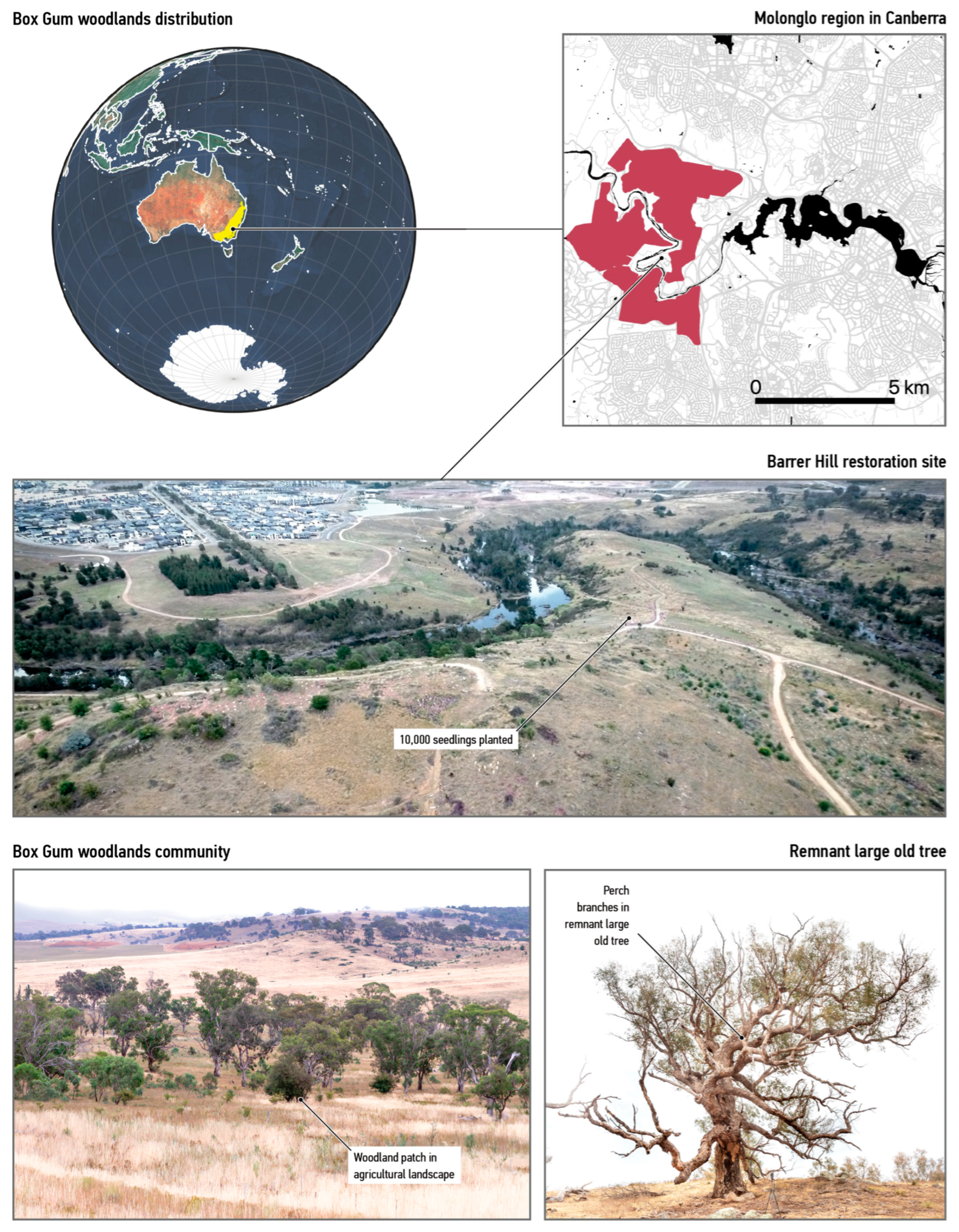
2.1. Use a Real-World Case

To provide a useful test case we compared strategies for supplying habitat features at the Barrer Hill restoration site in Canberra, Australia. This area is a severely degraded fragment of the box-gum grassy woodlands that covered most of south-eastern Australia before colonisation (Figure 1) [8]. These woodlands are dominated by widely spaced trees of the genus Eucalyptus such as yellow box (E. melliodora), apple box (E. bridgesiana), and Blakely’s red gum (E. blakelyi), with a ground layer comprising native tussock grasses and herbs. Less than 3% of the original extent of this ecological community remains [51].

We collaborated with partners who have been working to restore the site since 2011 [52]. Run by the Australian Capital Territory Parks and Conservation Service, the project seeks to improve current practices by developing artificial structures that more closely align with the preferences of arboreal wildlife. This case study serves as a design experiment [53] that grounds our theoretical work.

The prognosis for box-gum grassy woodlands is not encouraging. Policymakers and ecologists define such ecosystems as areas with large, old, and widely spaced trees [54]. The number of these trees is rapidly declining [55]. Models predict that millions of hectares will be without old trees within a few decades [7].

Development activity occurs within and adjacent to this woodland fragment. Thousands of new houses are already under construction [52]. Aiming to offset this damage, our collaborations worked to restore a 440-hectare degraded site called Barrer Hill (Figure 1). Restoration efforts have resulted in the planting of 10,000 new seedlings since 2012 [11]. Given that these young plants will not provide suitable habitat features for hundreds of years [11], the arboreal wildlife will have to depend on other forms of support.

Habitats of nationally and regionally significant species that rely on old trees are still present in the surrounding area [56]. To assess future impacts, we examined the behaviour of birds. We surveyed birds in the region twice per year over two years (2017 and 2019) at 72 trees [57]. The study observed birds using tree branches during 20 min intervals each spring over four years (see Supplementary Materials).

To model the use of habitat features, we focused on the availability of perch sites for birds. These sites are branches that birds visit for nesting, foraging, and observation. We focused on such branches because many birds, including Passerines, spend most of their lives perched in larger and older trees [58]. As discussed in the introduction, complex branch patterns are difficult to quantify without high-fidelity data and computational analysis [21,59].

To compare perch behaviours on different structures, we considered habitat features provided by living trees as well as manufactured beams and platforms [60]. Enriched utility poles with elevated perches and nesting platforms as well as snags have increased local bird abundance and species richness [11]. The structures provide examples of habitat features for numerical modelling.

2.2. Define Integrated Supply of Habitat Features

This section introduces the notion of supply. We use this term to denote any process that can produce habitat features. Examples include tree growth, microorganismal impact on wood, and manufacturing of objects by humans. We use the term ‘supply’ to emphasise constructive activities that produce habitat features. It encompasses innovation, making, and siting done by nonhuman as well as human engineers.

This use of ‘supply’ is not without precedent. For example, ecologists discuss the supply of cavities by trees [9,61,62]. This concept can highlight important dynamics such as time lags when habitat features result from revegetation [63] or thresholds in habitat production that can lead to the extirpation or extinction of species in managed forests [64]. These considerations extend to the discussion of eco-cultural interactions—for example, in forests [65].

Borrowing from economics, the term ‘supply’ is also common to the framework of ecosystem services for human use [66]. Examples include analyses of discrepancies between supply and demand [4,5] or for the identification of productive zones [67]. Despite their broad use, ecosystem-service approaches have received criticism for their anthropocentrism [26] and consequent portrayal of nonhuman beings as passive constituents [68]. In contrast, we use the term ‘supply’ to demonstrate the exceptional value of nonhuman contributions.

2.2.1. Define ‘Supply’ in Terms of Three Scales: Spatial, Organisational, and Temporal

One of the main challenges in the study of ecosystems is the integration of processes across scales [69,70,71]. To test our model’s ability for such integration, we introduced three scales: spatial, organisational, and temporal [72]. Here, our purpose was to capture differences within the scales.

We constrained the model via the analysis of physical objects that are meaningful to birds. We also included further data describing supply characteristics across the three scales (

Table 1. Phenomena and observations.

Scale	Process	Data
Spatial	Physical structures exhibit characteristic shapes, sizes, and features.	Custom workflow extracting branch information from manufactured and living habitat structures Restoration plans [52]
Organisational	Birds recognise structures as habitat features.	Observations of bird–branch interactions and structural properties of branches obtained via computational-feature extractions (see Organisational Scale Results in Section 3.1.2) Evidence of bird preferences for branches [5,73]
Temporal	Habitat structures exhibit characteristic development patterns, renewal cycles, and disturbance events.	Life-cycle analysis estimating lifespans and costs of built structures [74,75]. Ecological studies quantifying the density of trees in landscapes, mortality rates, renewal processes, and other dynamics [11,23]

).

We organised the outcome in the Section 3 following this pattern of three scales.

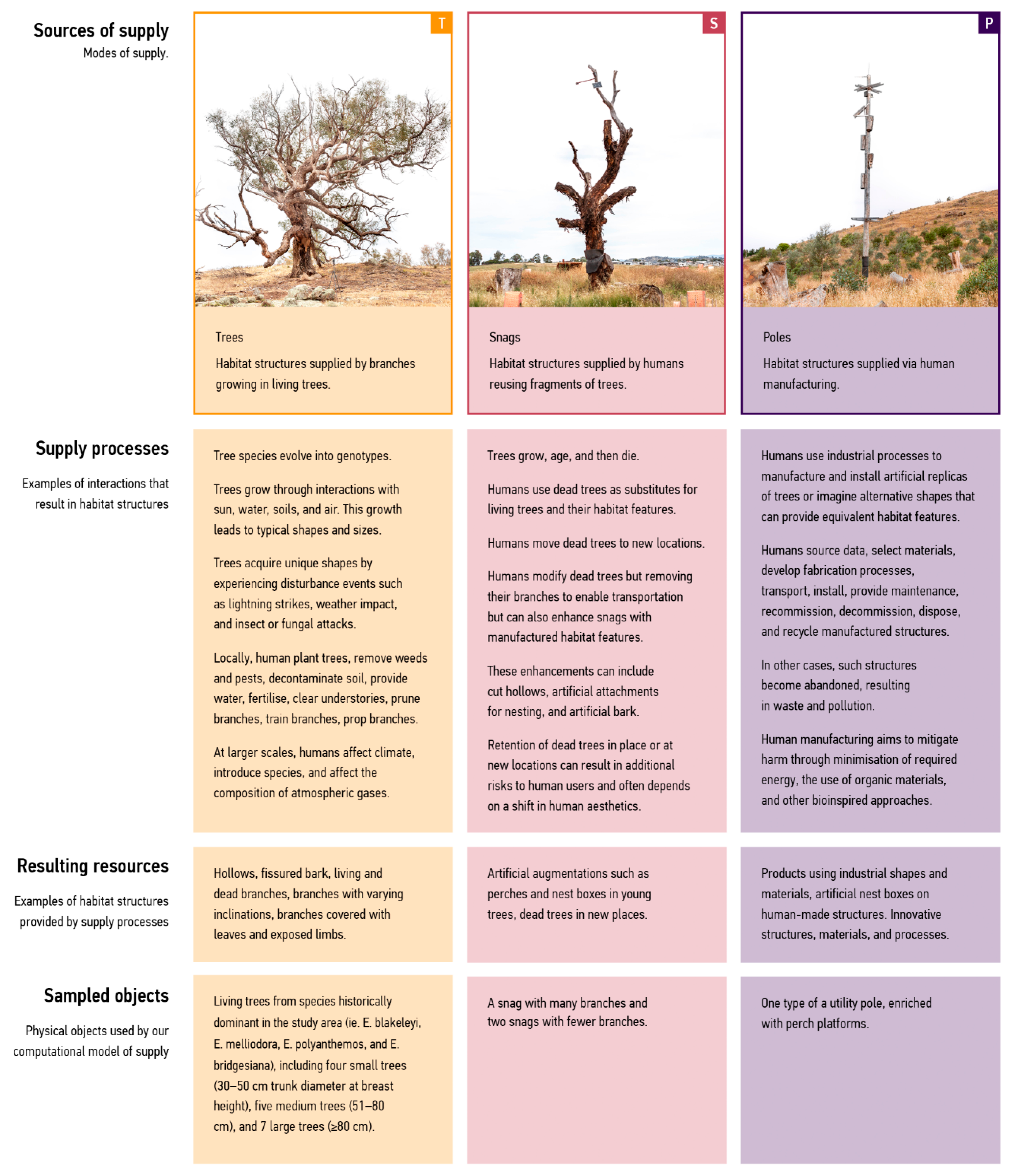
2.2.2. Define ‘Trees’, ‘Snags’, and ‘Poles’ as Three Modes of Supply

We next divided all sources of habitat features into three modes. As with scales, this division is simplistic but can serve to illustrate the comparability of habitat features within one model. These modes align with remedial measures proposed by the niche construction discourse in application to spatial niches [76]. This interpretation accepts that ecosystem engineers might be replaceable with biological or manufactured equivalents. Mapping to the possible actions, the modes of supply include:

• Mode 1—Trees: increasing numbers of key engineers (by planting trees that can supply branches for perching);
• Mode 2—Snags: increasing activities of key engineers (by reusing dead trees known as snags);
• Mode 3—Poles: introducing artificially engineered products (by installing utility poles supplied via human manufacturing).

Figure 2 introduces the modes of supply and links them to examples derived from the case study.

The rows in Figure 2 include examples of interactions resulting in supply, physical traces of these interactions that can provide habitat features, and sample objects used by our computational model. The purpose of this mapping was twofold: (1) to capture differences and nuances across all modes of supply irrespective of their source, as discussed in the Section 3, and (2) to indicate the implications for design, as described in the Section 4.

2.3. Describe the Model

We now describe a model that simulates supply modes using an adapted interpretation of the Overview, Design concepts, and Details (ODD) protocol [77].

2.3.1. Purpose and Patterns

The purpose of the model is to compare the dynamics of supply across modes.

2.3.2. Entities, State Variables, and Scales

The model implements habitat structures as a distribution of agents within a boundary. The model has two main components grouped under the headings with grey backgrounds in

Table 2. Model variables.

Variable	Units	Description
Agent Variables
Mode	Type	Supply mode (Snags, Poles, or Trees)
Age	Years	Variables that are common to all agent types
Location	X, Y coordinates
Unit cost	AUD
Service life	Years
Has been terminated	Boolean
Length of all branches in an agent	Metres	Habitat resources supplied by individual agents
Length of all dead branches	Metres
Length of all lateral branches	Metres
Length of all perch branches in an agent	Metres
Girth diameter	Metres	An equivalent to trunk diameter at breast height for trees. This variable differs between modes: tree agents can grow, snags and poles cannot.
Environment Variables
Boundary	GIS polygon	Site boundary that yields the area
Budget	AUD	Total funds for agents in one simulation
Strategy	List of routines that manage agent populations and a list of statistical weightings that influence probability rang	Management actions
Supply	Metres/year	Cumulative length of total branches and perch branches

: agents and an environment. Agents can undertake actions constrained by probabilities. The model initialises and controls agents through an environment that seeds initial values based on field observations and design decisions. At set intervals, the environment initialises and terminates agents, triggers agent actions, and calculates cumulative habitat features.

2.3.3. Process Overview and Scheduling

The model uses six processes to cover a representative period of supply (

Table 3. Model processes.

Process	Description	Run Time
Agent Actions
Survive	Increase ‘age’ by one Check if ‘age’ is less than ‘service life’, terminate if not.	Once per loop
Grow	Increase ‘girth diameter’ in tree agents based on a probability range.	Once per loop
Supply	Calculate the lengths of four branch types. Agents select resources randomly from a resource distribution calculated for each mode.	Snags and Poles run this process once when the environment runs ‘Initialise’ or ‘Renew’. Tree agents run this process after calling their ‘Grow’ process.
Environment Processes
Initialise	Define a strategy by setting variable values and renewal capabilities. Create the first generation of agents and set their variables.	At model initialisation
Renew	Create additional generations of agents.	Periodically, as defined at initialisation
Terminate	Terminate tree agents based on a probability range.	Once per loop
Update	Run agent actions.	Once per loop
Assess supply	Calculate lengths of branches by summing the lengths of all agents per mode. Remove terminated agents.	Once per loop

). Eucalyptus trees in the region become large enough to supply habitat features after approximately 175 years [11]. We selected 240 years as a representative period that we observed to be sufficient for the model to establish distinct trends.

The implementation uses an annual loop. Each year:

• Agents execute ‘Survive’;
• Tree agents execute ‘Grow’;
• Tree Agents execute ‘Supply’;
• Newly instantiated Snag and Pole Agents execute ‘Supply’;
• Environment executes ‘Terminate’;
• Environment executes ‘Assess Supply’;
• At some years, Environment executes ‘Renew’.

2.4. Model Supply

The model links tree growth and bird behaviour with design decisions.

2.4.1. Constrain Supply

We first listed operations that convert numerical assessment of habitat features and their use by birds into probability ranges that limit the actions of the agents (

Table 4. Dataflow for predicting resource distributions.

Operation	Resulting Data
Scan and model the shapes of habitat features.	Point clouds and polygonal meshes
Use feature-recognition algorithms to extract structural attributes.	Connected lines and their attributes
Use observational data to develop statistical models that estimate perch branches in sample structures.	Lengths of branches as extracted from scanned data
Link individual measures to define ranges of possible quantities of perch branches per mode.	Probability distributions representing likely perch branches
Make agents select values from within probability distributions.	Predicted branch lengths per agent

).

2.4.2. Controlling Supply through Strategies

Human users can influence the model by adjusting probability values within evidence-based ranges.

They can:

• Allocate budget for each supply mode;
• Assign weights to probability ranges used for ‘Terminate’, ‘Supply’, and ‘Renew’ agent actions, as well as to the ‘unit cost’ variable;
• Choose to run or disable the ‘Renew’ action.

Combinations of these values constitute design strategies that impact supply. We examined strategies for each supply mode, representing plausible design decisions and marginal cases:

• The ‘Plant Trees’ strategy uses only the Tree mode, with default probability ranges for agents and the ‘Renew’ process disabled.
• ‘Plant, Maintain, and Renew Trees’ lowers the ‘Terminate’ probability range for agents and enables ‘Renew’, considering conservation guidelines from Gibbons et al. [23].
• ‘Plant, Maintain, and Renew Trees; Source as Cheaply as Possible’ lowers the ‘Terminate’ probability range, enables ‘Renew’, and increases agent populations by using lower probable ‘unit cost’ values.
• ‘Plant, Maintain and Renew Trees; Install Poles’ uses Tree and Pole modes (see

  Table 5. Strategies and model attributes.

  	Budget Allowances			Distribution Weightings
  Strategies	Trees	Snags	Poles	Unit Cost	Supply	Terminate	Renew
  Plant Trees	100%	0	0	Average	Average	Low	No
  Plant, Maintain, and Renew Trees	100%	0	0	Average	Average	High	Yes
  Plant, Maintain, and Renew Trees; Source as Cheaply as Possible	100%	0	0	Low	Average	High	Yes
  Plant, Maintain, and Renew Trees; Install Poles	50%	0	50%	Average	Average	Average	Yes
  Plant, Maintain, and Renew Trees; Install Poles Sourced Cheaply as Possible	50%	0	50%	Low	Average	Average	Yes
  Plant, Maintain, and Renew Trees; Install Snags	50%	50%	0	Average	Average	Average	Yes
  Plant, Maintain, and Renew Trees; Install Snags; Retain Snag Branches	50%	50%	0	Average	High	Average	Yes
  Plant, Maintain, and Renew Trees; Install Snags; Retain Snag Branches; Source Snags Cheaply	50%	50%	0	Low	High	Average	Yes

  budget allocations), with default probability ranges for pole agents and tree agents parameterised as in ‘Plant, Maintain and Renew Trees’.
• ‘Plant, Maintain, and Renew Trees; Install Poles Sourced as Cheaply as Possible’ uses Tree and Pole modes while accounting for potential supply effects from economies of scale by lowering probable ‘unit cost’ values for pole agents.
• ‘Plant, Maintain, and Renew Trees; Install Snags’ uses Tree and Snag modes, with default probability ranges for snag agents and parameters from ‘Plant, Maintain and Renew trees’ for tree agents.
• ‘Plant, Maintain, and Renew Trees; Install Snags; Retain Branches’ uses Snag and Pole modes, increasing the ‘Supply’ probability range for snag agents to simulate potential supply improvements through possible retention of tree limbs during removal and transportation.
  ‘Plant, Maintain, and Renew Trees; Install Snags; Retain Branches; Source Snags Cheaply’ is a marginal case that implements trees and high-performing snags by increasing the ‘Supply’ probability range and lowering the ‘unit cost’ probability ranges in snag agents.

Table 5 outlines actions used in alternative strategies.

To compare the simulated strategies and their supplies of perch branches over the simulated period, we ran each strategy 30 times. We describe outcomes of this model and the simulated strategies in the Section 3.

3. Results

Our results demonstrate that available sources of data can:

• Unify heterogenous modes of supply in one model;
• Capture differences between modes of supply;
• Predict consequences of design decisions.

The following sections describe these results.

3.1. Model of Supply across Modes

This section presents examples of model outputs, with further detail in the Supplementary Materials. For each scale, we included: (1) the character of the processes, (2) key challenges, (3) model capabilities to overcome these challenges, and (4) the comparative analysis supported by the model.

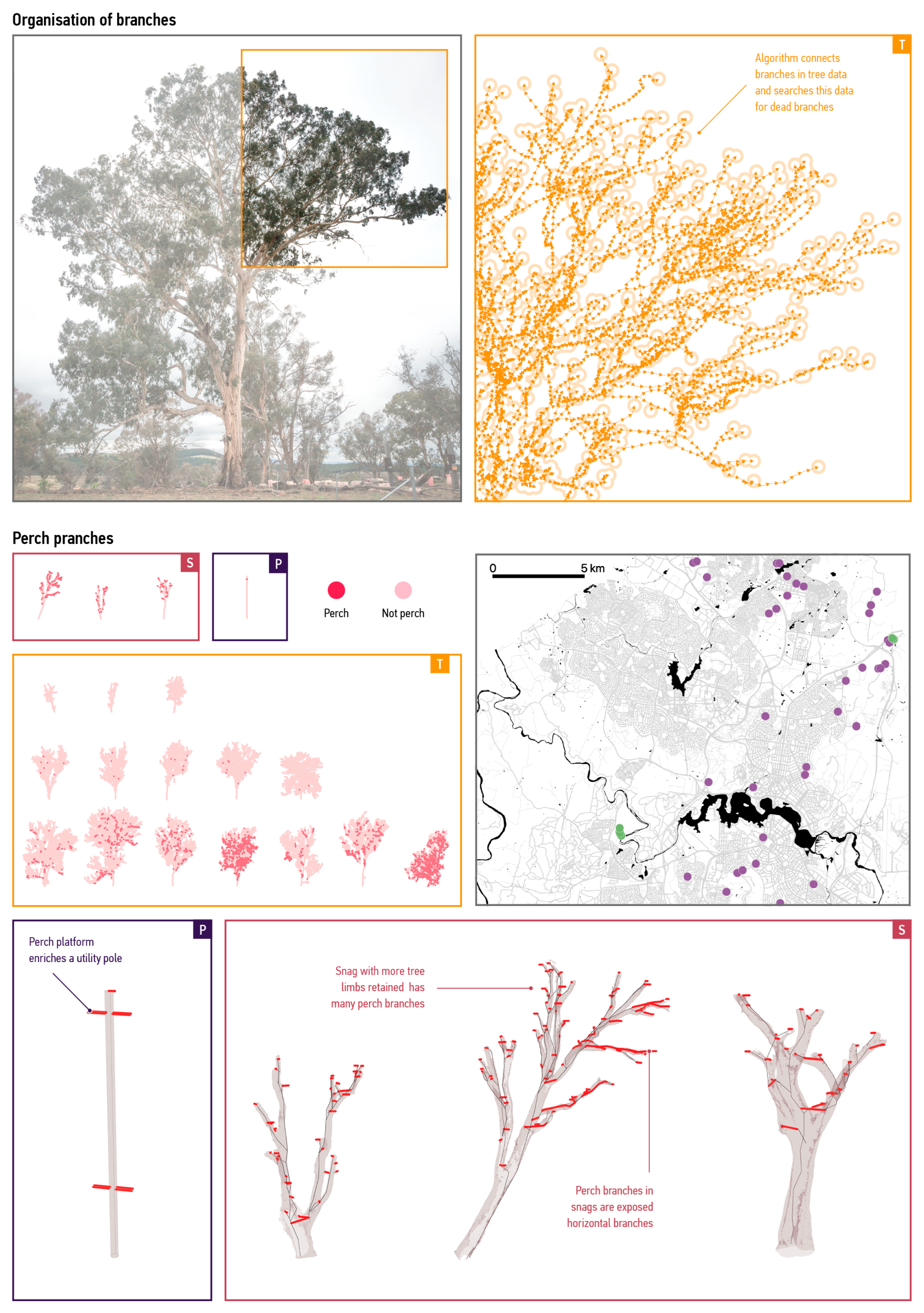
3.1.1. Spatial Scale

The model works at spatial scales that range from cubic metres to hectares. For instance, in landscapes, habitat features are implicated in human and nonhuman interactions that can be difficult to study. The model addresses this challenge by linking spatial and economic factors. We defined the site as a 400-hectare bounded region [52] and derived numbers of agents by relating their costs to funding allocated for site rehabilitation. Prices for utility poles ranged from AUD 1968.38 in industrial estimates [74] to AUD 16,815, as observed in field experiments [11]. The same field experiments suggested AUD72–144 for tree saplings and AUD4049–24,294 for snags, with lower numbers representing our estimate for possible optimisations. The model can help human users to consider relationships between economic and geographical constraints and choose better design strategies.

Spatial processes within tens of cubic metres lead to ecologically important complexities. Here, we illustrate processes that occur within the range of cubic meters because current quantitative approaches do not address such interactions, as discussed in the Section 1. Our data processing standardised habitat features supplied by all modes into branch-like segments between 0.2 m and 0.5 m in length (Figure 3).

With this approach, we obtained between 351 and 11,217 (mean: 4875) branch segments in trees, 262–656 (mean: 265) branch segments in snags (n = 3), and 80 branch segments in utility poles (n = 1). Different modes required distinct extractive approaches. In the case of trees, we used feature-extraction algorithms to remove leaves [78], fit line segments to the remaining branches [79], and differentiate such segments based on their exposure, horizontality, and proximity to other structures. To extract these segments in snags, we manually traced branches on polygons using the modelling program Rhinoceroses. An automated procedure used for trees could work here but was not necessary because of the relative simplicity of these structures. Quantities of segments in the most branch-rich snag only exceeded those in our three smallest tree samples (trunk diameters 27–41 cm), showing the complexity of tree canopies compared to other modes. We could automatically generate branch segments from a list of lengths and orientations for utility poles manufactured from standard components. This representation of all branch-like habitat features as one computational type—a branch segment—creates an approach that can compare quantities, exposures, sizes, and geometries for all modes.

3.1.2. Organisational Scale

Constructed habitats can lead to the creation of useable ecological niches that nonhuman species fail to recognise. For example, the patterning of branches can affect habitat characteristics of tree crowns but is difficult to study. The model engaged with this challenge by considering how organisational characteristics result in features that birds recognise as suitable (Figure 4).

Perching behaviour is common to many bird species [73,80,81]. For this model, we followed approaches that use composite indicators [82,83] and assessments of tree-related microhabitats [84] and considered such birds as one virtual taxon. This approach can be differentiated to account for distinct species in subsequent work.

To develop this evaluation procedure, we analysed a database that recorded observations of perching birds to identify structural properties correlated with increased bird visits (Figure 4, top-right) and used this information to quantify perch branches in the sampled structures (Figure 4, top left) (see Supplementary Materials Section S1), for further details). We extracted 0–155 m perch branches per sampled tree using the branch characteristics discussed in the previous section. For example, to identify likely bird presences, we preserved branch hierarchies in trees by encoding detected branches as connected graphs and used this information to identify dead branches (Figure 4, middle).

We also differentiated snag and utility-pole branch-like elements based on orientation and identified likely bird presences using branches with an angle < 20° relative to the horizontal plane. We obtained 10–43 m perch branches per sampled snag and 3 m of such branches in utility poles (Figure 4, bottom). These results demonstrate that computational models can capture meanings of physical objects for nonhuman inhabitants.

We will now elaborate on the results that pertain to the organisational range of individual tree-like structures. The model considered how formation processes lead to typical shapes, identities, and sizes of such individuals.

We organised the branch segments in trees, utility poles, and snags to obtain characteristic trends that constrained the agents’ ‘Supply’ actions (Figure 5).

For trees, we plotted samples by age and trunk diameter and linked measured quantities using a LOESS regression (see Supplementary Materials Section S2 for details, including the selected smoothing parameters). This operation showed the nonlinear relationship between growing trees and the supply of perch branches (Figure 5, top and middle orange curves).

By contrast, the lengths for snags assumed no relation between samples. This reflects the likely availability of perch branches in collections of snags found by chance. We quantified branch lengths in utility poles as a single point (the measurements obtained from the pole sample), reflecting the ability of industrial manufacturing to produce structures of exact dimensions (Figure 5, bottom curves). By defining the organisation of measured quantities, the model accounted for the characteristic patterns of supply originating in trees, snags, or manufactured structures.

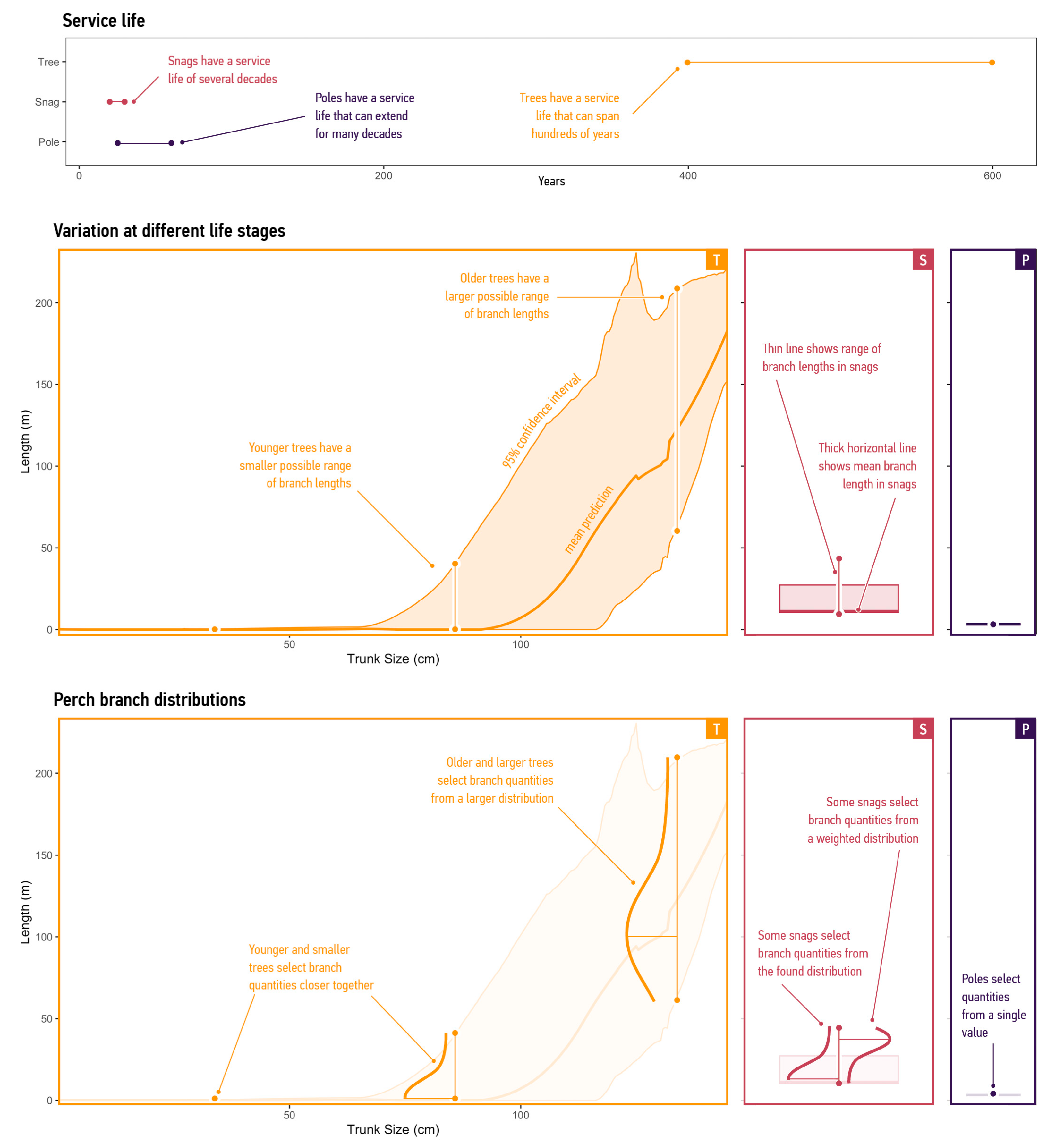
3.1.3. Temporal Scale

Finally, the model considered temporal ranges, including renewal of natural and artificial habitat structures. Humans control such processes in managed landscapes, and they can extend over many decades. To account for these processes, we quantified recruitment and recommissioning for each mode, including regeneration pulses for trees every 30 years according to the guidelines produced by previous modelling [23].

In constructed ecosystems, rapid changes can disrupt trends. For example, human construction can quickly install snags and poles with perch branches (within weeks or months), whereas trees need to grow and experience disturbance events such as lightning or fungal attacks before they can produce useable branches. To estimate the rate at which trees acquire unique shapes and structure, we used annual trunk-growth estimates ranging from 0.37 to 0.51 cm in yellow-box trees (E. melliodora) [23,85,86], one of the historically dominant species of this ecological community. The model also considered the risk of sudden termination of habitat structures by removing 0.01–0.003% of trees each year, as defined by previous modelling [23]. Accounting for outcomes at this temporal range allowed the model to compare instantaneous and extended interactions.

We discuss the results related to the temporal range of centuries in more detail below, because typical project durations rarely extend to cover multiple generations of large old trees (Figure 6).

To account for variation, we quantified life stages for each mode. We began by providing a common frame for the life-cycle durations of habitat structures (Figure 6, top graph). In the study area, dominant Eucalyptus trees have a lifespan ranging from 400 to 600 years [85], and research has indicated that trees can remain upright for an additional 50 years after death [57]. Life-cycle assessments, which model material choices for common utility poles, provide a service-life range of 25–60 years for these steel, concrete, and wood-veneer structures [74]. There are no ready life-cycle estimates for translocated snags. Therefore, we assumed that the service life of this mode is similar to that of other engineered vertical structures and estimated the service life to be 20–30 years. This is comparable to the estimates for wind turbines [75]. These results engage with the extended temporal ranges that will be necessary for effective management.

The model evaluated the influence of temporal events on modes by obtaining characteristic probability distributions of perch branches. These distributions constrain agents’ ‘Supply’ actions. For trees, the model obtained confidence intervals for measurements to define a truncated normal distribution of perch branches that changes as trees progress through life stages (Figure 6, orange bell-shaped curves in bottom graph). To specify these distributions, the model used a bootstrap-resampling method to obtain confidence intervals for the regression curve linking measured samples by age [87]. We used this method to resample the original data 10,000 times to obtain a likely distribution. Snags had probability distributions determined by the range of measured samples (Figure 6, pink bell-shaped curves in bottom graph) and poles had a distribution that was a single value (Figure 6, purple bell-shaped curves in bottom graph).

The model used these data to produce a numerical estimation of variations in perch branches caused by accumulations of chance events. Younger agents select resources near the median value, whereas agents representing older and larger trees choose perch-branch quantities from a larger probability distribution. For instance, the distribution for a tree agent with a 50 cm diameter trunk had a standard deviation of 1.01 m, whereas the distribution for an agent with a 100 cm diameter trunk had a standard deviation of 74 m.

For other modes, the model modified weightings of distributions to incorporate variations resulting from human design strategies. For instance, we assumed that variations in snags result from humans removing branches during transportation. Therefore, snag agents under the ‘Plant, Maintain, and Renew Trees; Install Snags; Retain Branches’ strategy chose perch-branch quantities from a truncated distribution, allowing the model to capture variations in perch branches resulting from human action (Figure 6, bottom-right graph). This functionality illustrates the potential for integrated modelling of supply patterns determined by growth and disturbance processes as well as those restricted by human activities.

3.2. Supply Predictions

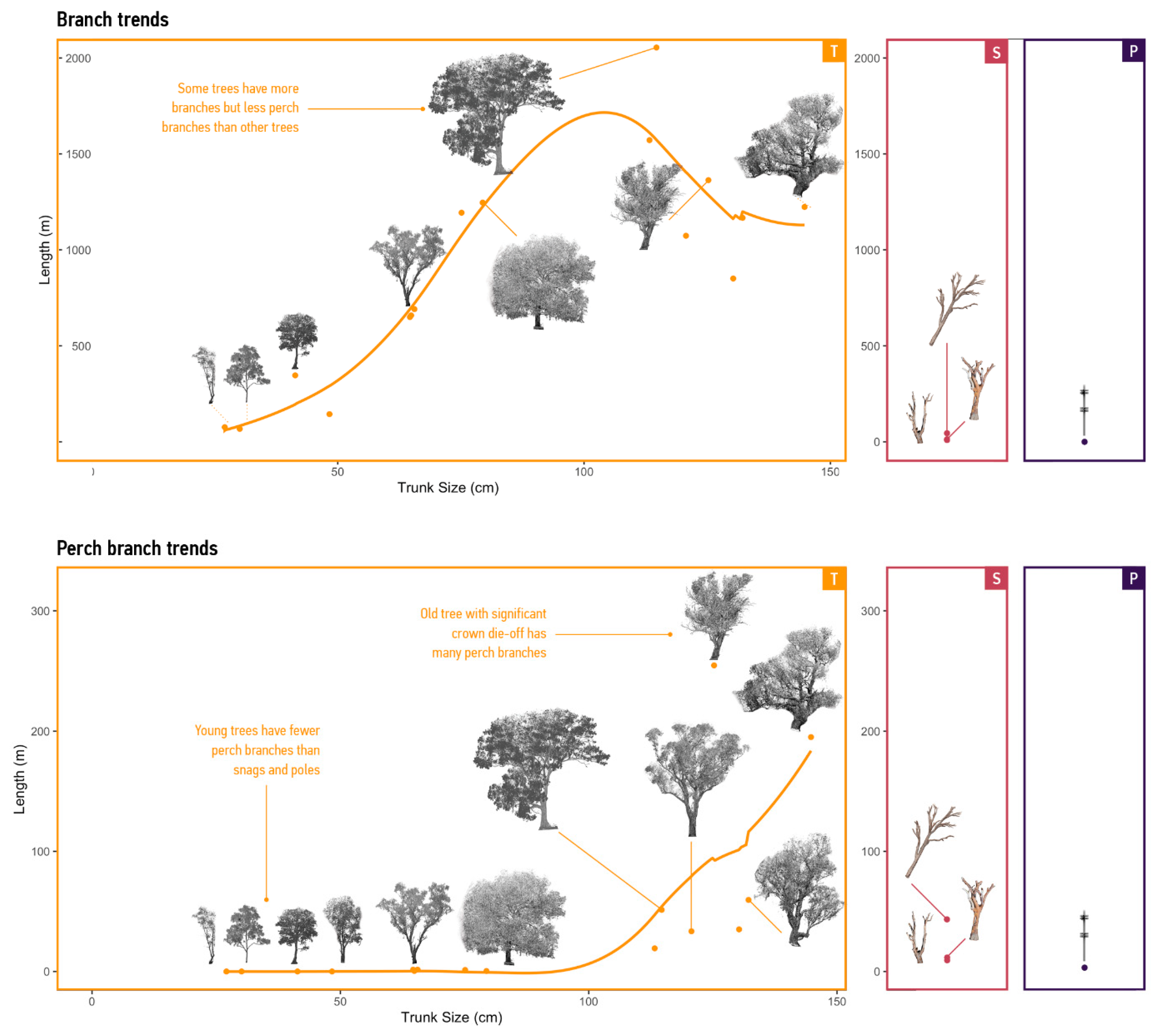
3.2.1. Supply of Branches

We now present the outcomes of the simulations. We first demonstrate that the model could calculate quantities of habitat structures over time. To provide an example, we focus on trees because that supply mode is more complex. Using settings grouped under the strategy ‘Plant, Maintain, and Renew Trees’ (see Methods), Figure 7 shows predicted quantities for different branch types, illustrating the changing availabilities of total branches.

In Figure 7, the rows correspond to different types of branches, and the squares correspond to two-year intervals. The colour of the cells represents the predicted supply of branches in this interval. The simulation makes clear that trees begin supplying branches at year 1. Dead branches appear later and become distributed throughout the site after year 60. Perch branches are the last to become available, at year 120, the next measured interval, with distribution throughout the site appearing at year 180 and significant quantities only appearing at year 240.

The simulation also quantified branch types supplied by trees. Integrating 30 simulation runs, at year 240 trees provided, on average, 4,490,892 m of branches, 246,263 m of dead branches, and 23,246 m of perch branches. These numbers emphasise the significant quantities of habitat features provided by trees, highlighting the capabilities of the model. These results also confirm that trees supply useful perch branches late in life, indicating the need for manufactured replacements.

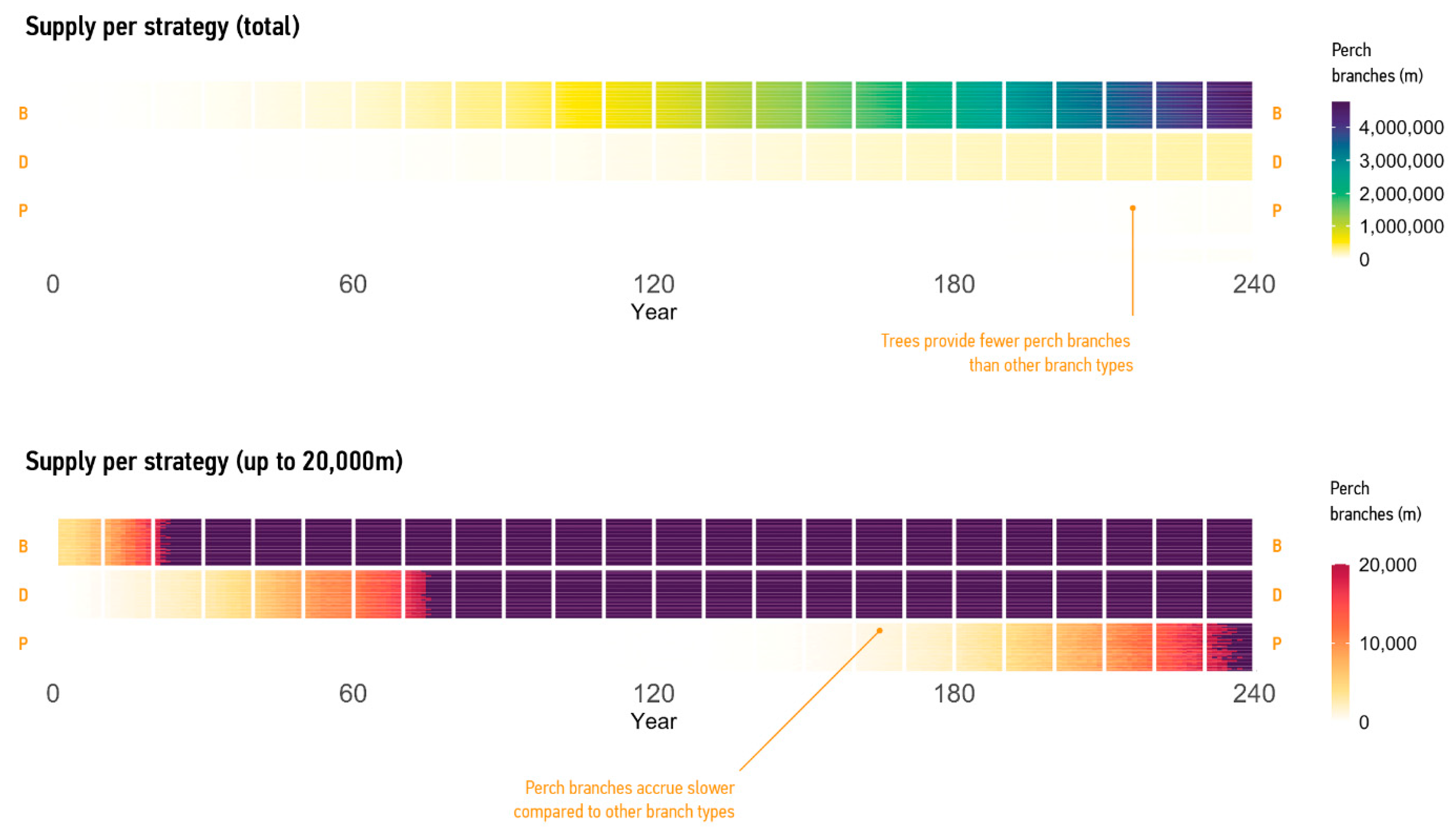
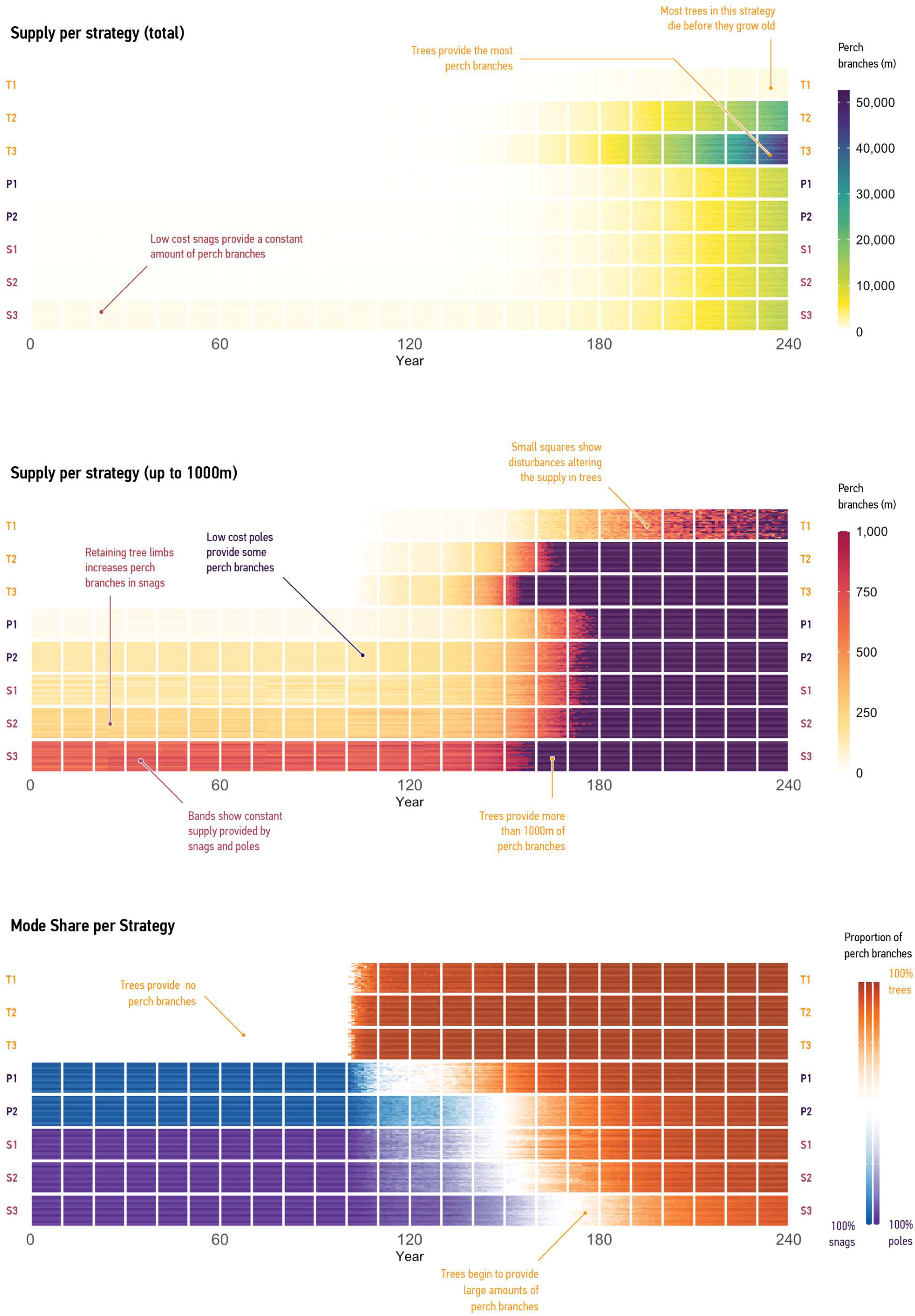
3.2.2. Supply per Mode

Finally, we present the supply of habitat resources provided by modes. We grouped the outcomes of the simulations as cumulative lengths of perch branches per mode (Figure 8).

The results quantify the supply effects under various strategies. For example, the model predicted that tree agents would supply 1.1 km of perch branches at year 240 under ‘Plant Trees’. Conversely, under the ‘Plant, Maintain, and Renew Trees’ and ‘Plant, Maintain, and Renew Trees; Source as Cheaply as Possible’ strategies, the model forecasted a supply of 22.9 km and 46.1 km of perch branches, respectively, at year 240. However, all strategies relying on trees as the primary mode for perch branches exhibited almost no supply for a minimum of 150 years.

In contrast, strategies that involve snags maintained a constant supply of perch branches, providing an average of 157–709 m. Strategies that incorporate utility poles maintained supply at a lower rate, between 34–157 m of perch branches. These results suggest that despite providing significantly lower quantities of perch branches than fully grown trees, the modes of supply that incorporate artificial habitat structures can meaningfully add to the totals. The subsequent section discusses the implications of these strategies.

4. Discussion

This study used modelling to support design decisions in degraded landscapes where human intervention is necessary to preserve numerous species. We employed the concept of supply to integrate diverse sources of habitat features. There is a lack of such approaches in urban ecosystems, as evidenced by a recent meta-analysis of artificial habitat structures [29] and studies of measurement capabilities [88]. To address this gap, we considered three modes and three scales.

Here, we (1) discuss our model’s ability to analyse ‘natural’ and ‘artificial’ structures together, (2) its ability to provide better predictions, and (3) its potential to inform design strategies.

4.1. Benefits of Integrated Supply Models

In this section, we discuss the advantages of an integrated model that incorporates diverse supply modes. We used a flow diagram to illustrate the advantages of our approach (Figure 9).

We relied on lidar data to extract surfaces and lengths (see Figure 3), and this approach excluded some important arboreal-habitat features, such as hollows, flowers, leaves, epiphytes, and peeling bark [16,89,90]. We also did not consider potentially negative impacts of habitat features, as observed in ecological traps [91].

Despite these simplifications, our model demonstrates that integrative approaches can result in sustainable supply. Our finding, that trees will not supply perch branches for at least 150 years (see Figure 7), agrees with existing models’ projections about the future of large old trees and other age-related structures like nesting hollows [11,23]. Supply must therefore integrate functionalities provided by living trees, dead trees, and artificial structures such as utility poles or possible custom-designed enhancements.

Research on smart infrastructures highlights the necessity for complex living communities to incorporate diverse information sources, including new data and community-member participation [92,93]. In such settings, human designers act as external experts who can guide supply flows (Figure 9, triangles). At times, this guidance can successfully provide perch branches, as evidenced by larger loops in each mode. However, it can also result in supply failures (Figure 9, abridged loops indicated by dashed lines), such as when human interventions disrupt vital processes needed to maintain old trees and ensure tree recruitment.

In such circumstances, numerical measures derived from our model reduce uncertainty about nonhuman activities. For example, our method can estimate the significance of habitat features based on bird perceptions. In Figure 9, green dashed regions represent bird capabilities, with the surrounding areas representing additional factors such as epigenetic effects, phenotypic plasticity, and behavioural adaptations. We concentrate on the two defined regions to indicate bird behaviour. Birds’ use of habitat features depends on their physiological characteristics, as well as their perceptual and cognitive capabilities. Successful use of habitat features occurs in the overlap between these two sets.

Our approach highlights interrelated interactions across modes, as well as opportunities for hybrid modes of supply that occur, for example, when humans augment utility poles with manufactured perches or use dead trees in new locations (Figure 9, arrows changing colours). We will now discuss how our model compares to other models in evaluating these systems.

4.2. Current and Possible Predictions

Assessments of heterogenous supply systems depend on analysis across scales. We will now discuss such scales and compare our model with existing approaches, focusing on three aspects described in the Section 1: detail, range, and dynamics (

Table 6. Comparison of the model with existing approaches.

Aspect	State of the Art	Benefits of Our Approach	Opportunity for Further Work
Detail	Informed by coarse resolution the aerial-lidar and other remote-sensing methods [50]. Assesses generic habitat features and typical shapes [11,23].	Informed by higher resolutions of the terrestrial lidar. Assesses individual branch-like structures of any kind.	Includes additional habitat features such as hollows, peeling bark, and coarse woody debris.
Range	Can represent trees as simple shapes over extended periods [94] or represent detailed tree structures over short time spans [95,96]. Uses limited spatial and temporal ranges to assess artificial structures [29].	Can represent detailed habitat features over time. Compares across extended ranges.	Models in response to geography and interactions within groups of habitat structures.
Dynamics	Evaluates strategies providing diverse habitat structures using opportunistic tools [97]. Considers individual events or strategies with limited scope for comparison [98].	Evaluates strategies offering varied habitat structures in relation to bird utilization of features. Can assess and compare long-term trends.	Consider embodied energy and other properties of materials. Consider constructability and adaptability of structures.

).

Our approach captures additional detail by using terrestrial-lidar data. The use of lidar is more common in recent ecological simulations [50]. However, these simulations usually use aerial lidar, which has resolutions of tens of points per meter, in contrast to the hundreds of thousands of points per meter provided by terrestrial-lidar devices [49]. The enhanced detail afforded by these data allows us to model spatial capacity such as branch lengths, physical arrangements such as branch connectivity or orientation, and component identity such as the living or dead states of branches. This approach helps to overcome a known constraint where available tools limit the evaluations and planning of restoration projects [97].

This enhances previous simulations of scattered large old trees, including yellow box (E. melliodora) [11,23], as well as perch-site modelling in trees [47,99,100], by broadening the concept of a branch to include various living and manufactured habitat structures that can provide relevant functions (see Figure 4).

Some ecological models do focus on individual tree traits and simulate their behaviours over hundreds of years [94]. However, such models represent tree shapes as simple volume boundaries. This approach does not provide sufficient information for the differentiation of branches within tree crowns and simulations of their meaning for birds [33]. Models that depict trees as three-dimensional structures, such as functional-structure models [95,96], are also not suitable for assessing perch branches because they focus on typical growth patterns and do not include stochastic events that determine shapes of older individual trees, which we include.

Spatial and temporal ranges of numerical analyses applied to artificial structures are also narrow, with most studies focusing on centimetre to metre spatial ranges and rarely extending beyond the temporal range of 12 months [29]. Our model extends such approaches by supporting the exploration of long-term trends.

Life-cycle assessments are common in the evaluation of industrial products and buildings. Some recent versions, such as life-cycle assessments for sustainability [98] or biodiversity [27], suggest future extensions for our modelling. Relevant capabilities might track carrying capacity, embodied energy, sequestered carbon, and other factors. In comparison, the advantage of our model is its ability to account for hundreds of years, the temporal range that typical life-cycle assessments do not attempt.

Although this article only considers costs per structure, it can serve as a template for future research that might consider embodied energy, material usage, and other factors such as constructability or adaptability, as already attempted for artificial reefs [31]. Better numerical understanding of habitat structures can be important for the assessment of their efficiency but also as the foundation for better design, as we discuss in the next section.

4.3. Potential to Support Design Strategies

This section highlights the potential of our modelling to enhance design that can support nonhuman inhabitants in degraded ecosystems. We discuss each strategy and its impact on supply (Figure 10).

The Trees mode shows strategies that aim to increase the number and performance of key engineers by planting trees that supply perch branches.

The ‘Plant Trees’ strategy, labelled T1, resulted in minimal perch-branch supply at year 240 due to high mortality rates and lack of regeneration. Most trees died before contributing to the supply.

In contrast, the ‘Plant, Maintain and Renew Trees’ strategy, labelled T2, addressed these issues by reducing tree mortality and increasing new tree supply through renewal events. This strategy increased perch-branch quantity by 21 times compared to ‘Plant Trees’, highlighting the importance of maintenance, renewal, and recommissioning for the Trees mode.

‘Plant, Maintain, and Renew Trees; Source as Cheaply as Possible’, labelled T3, shows the effect of doubling the tree-agent populations. Although there were more perch-branch quantities at the end of the simulation, we found that larger tree-agent populations did not impact supply for a considerable period. At years 30, 60, and 90, the supply under both Plant, Maintain, and Renew Trees; Source Cheaply’ (which doubled the number of tree agents) and Plant, Maintain, and Renew Trees’ was zero. By year 90, tree agents operating under either strategy provided only small amount of supply (a total of 0.08 m and 0.12 m, respectively). Our findings emphasize the limitations of tree-based supply and the need for augmentation, which can include methods that accelerate tree aging, reduce tree mortality, or allow trees to remain in place after they die.

Moving to the Poles mode, we examined strategies that modelled a possible increase in availability of habitat features when multiple modes of supply operate simultaneously.

‘Plant, Maintain and Renew trees; Install Poles’, labelled P1, shows the impact of unit costs on supply. Trees can provide the largest volume of branches, and tree saplings are inexpensive. However, trees grow slowly. In contrast, installing more manufactured structures at a lower unit cost leads to an immediate impact on supply. Because poles require less transportation and installation effort than other modes, this allows for minimal quantities of perch branches, with the supply spread across the site.

The ‘Plant, Maintain, and Renew Trees; Install Poles Sourced as Cheaply as Possible’ strategy, labelled P2, explored economies of scale that emerge from large-scale and persistent manufacturing. As a result, perch-branch supply rapidly increased from 34 m to 157 m (see Figure 9) compared to ‘Plant, Maintain and Renew Trees; Install Poles.’ This strategy highlights the impact of unit costs on supply, demonstrating the benefits of sourcing poles more affordably.

Shifting to the Snags mode, strategies can provide concentrated amounts of perch branches that have an immediate impact on supply.

‘Plant, Maintain, and Renew Trees; Install Snags’, labelled S1, yielded an average of 157 m of perch branches annually over the simulated period. ‘Plant, Maintain, and Renew Trees; Install Snags’ increased this supply to 247 m (see Figure 9). The contrast between the two snag strategies shows the potential of measures that aim to retain branches during transportation.

The ‘Plant, Maintain, and Renew Trees; Install Snags; Retain Branches; Source Cheaply’ strategy, labelled S2, provided the greatest supply for the first 150 years. It modelled the possibility of cheap snags. At these optimal conditions, snags remained on par with tree agents until year 160 (709 m), by which point trees would have developed 768 m of branches (see Figure 8). It is also important to note that trees rapidly exceeded this performance by year 180, when they would have accumulated 2417 m of branches. These trees continued to produce perch branches at an increasing rate until the end of the simulated period, clearly underlining their long-term superiority.

Although our research strongly confirms the outstanding value of old trees as habitat suppliers, we also note the evolved limitations of such structures and the possible opportunities for design. For instance, challenges with procuring and transporting large snags limited the ‘Plant, Maintain, and Renew Trees; Install Snags; Retain Branches; Source Cheaply’ strategy, labelled S3. Instead, designers can attempt to match the performance of snags through the provision of artificial structures that can supply similar amounts of perch branches while relying on easier transportation, construction, and installation. This scenario illustrates the connection between the availability of perch branches and possible design briefs for cost-efficient but large-spanning designs.

5. Conclusions

This study introduces a unique approach to modelling habitat supply in degraded landscapes, integrating diverse sources of habitat features. We address the challenge of combining living trees with dead trees and manufactured structures to ensure sustainable supply. Our model predicts the consequences of design strategies, capturing differences between modes of supply and unifying them into a single framework. Our results emphasize the limitations of tree-based supply and the need for augmentation with methods that accelerate tree aging, reduce tree mortality, or allow trees to remain in place after they die. Strategies that incorporate snags or utility poles maintain a constant supply of perch branches, providing a lower rate than fully grown trees but still adding to the total. Our research confirms the value of old trees as habitat suppliers while also highlighting the limitations of such structures and possible opportunities for design.

References

1. Prevedello, J.A.; Almeida-Gomes, M.; Lindenmayer, D.B. The Importance of Scattered Trees for Biodiversity Conservation: A Global Meta-Analysis. J. Appl. Ecol. 2018, 55, 205–214. [Google Scholar] [CrossRef]
2. Lewandowski, P.; Przepióra, F.; Ciach, M. Single Dead Trees Matter: Small-Scale Canopy Gaps Increase the Species Richness, Diversity and Abundance of Birds Breeding in a Temperate Deciduous Forest. For. Ecol. Manag. 2021, 481, 118693. [Google Scholar] [CrossRef]
3. Lindenmayer, D.B.; Laurance, W.F.; Franklin, J.F. Global Decline in Large Old Trees. Science 2012, 338, 1305–1306. [Google Scholar] [CrossRef] [PubMed]
4. Lindenmayer, D.B.; Laurance, W.F. The Ecology, Distribution, Conservation and Management of Large Old Trees. Biol. Rev. 2016, 92, 1434–1458. [Google Scholar] [CrossRef] [PubMed]
5. Gibbons, P.; Boak, M. The Value of Paddock Trees for Regional Conservation in an Agricultural Landscape. Ecol. Manag. Restor. 2002, 3, 205–210. [Google Scholar] [CrossRef]
6. Le Roux, D.S.; Ikin, K.; Lindenmayer, D.B.; Manning, A.D.; Gibbons, P. The Future of Large Old Trees in Urban Landscapes. PLoS ONE 2014, 9, e99403. [Google Scholar] [CrossRef] [PubMed]
7. Manning, A.D.; Gibbons, P.; Fischer, J.; Oliver, D.; Lindenmayer, D.B. Hollow Futures? Tree Decline, Lag Effects and Hollow-Dependent Species. Anim. Conserv. 2012, 16, 395–405. [Google Scholar] [CrossRef]
8. Lindenmayer, D.B.; Prober, S.; Crane, M.; Michael, D.; Okada, S.; Kay, G.; Keith, D.; Montague-Drake, R.; Burns, E. Temperate Eucalypt Woodlands. In Biodiversity and Environmental Change: Monitoring, Challenges and Direction; Lindenmayer, D.B., Burns, E., Thurgate, N., Lowe, A., Eds.; CSIRO: Colingwood, Australia, 2014; pp. 283–334. ISBN 978-0-643-10857-8. [Google Scholar]
9. Ibarra, J.T.; Novoa, F.J.; Jaillard, H.; Altamirano, T.A. Large Trees and Decay: Suppliers of a Keystone Resource for Cavity-Using Wildlife in Old-Growth and Secondary Andean Temperate Forests. Austral Ecol. 2020, 45, 1135–1144. [Google Scholar] [CrossRef]
10. Beyer, G.L.; Goldingay, R.L. The Value of Nest Boxes in the Research and Management of Australian Hollow-Using Arboreal Marsupials. Wildl. Res. 2006, 33, 161–174. [Google Scholar] [CrossRef]
11. Hannan, L.; Le Roux, D.S.; Milner, R.N.C.; Gibbons, P. Erecting Dead Trees and Utility Poles to Offset the Loss of Mature Trees. Biol. Conserv. 2019, 236, 340–346. [Google Scholar] [CrossRef]
12. Watchorn, D.J.; Cowan, M.A.; Driscoll, D.A.; Nimmo, D.G.; Ashman, K.R.; Garkaklis, M.J.; Wilson, B.A.; Doherty, T.S. Artificial Habitat Structures for Animal Conservation: Design and Implementation, Risks and Opportunities. Front. Ecol. Environ. 2022, 20, 301–309. [Google Scholar] [CrossRef]
13. Schnell, S.; Kleinn, C.; Ståhl, G. Monitoring Trees Outside Forests: A Review. Environ. Monit. Assess. 2015, 187, 600. [Google Scholar] [CrossRef]
14. Gustafson, E.J.; Kern, C.C.; Kabrick, J.M. Can Assisted Tree Migration Today Sustain Forest Ecosystem Goods and Services for the Future? For. Ecol. Manag. 2023, 529, 120723. [Google Scholar] [CrossRef]
15. Lindenmayer, D.B. Conserving Large Old Trees as Small Natural Features. Biol. Conserv. 2017, 211, 51–59. [Google Scholar] [CrossRef]
16. Le Roux, D.S.; Ikin, K.; Lindenmayer, D.B.; Bistricer, G.; Manning, A.D.; Gibbons, P. Enriching Small Trees with Artificial Nest Boxes Cannot Mimic the Value of Large Trees for Hollow-Nesting Birds. Restor. Ecol. 2015, 24, 252–258. [Google Scholar] [CrossRef]
17. Gibbons, P.; Lindenmayer, D.B. Offsets for Land Clearing: No Net Loss or the Tail Wagging the Dog? Ecol. Manag. Restor. 2007, 8, 26–31. [Google Scholar] [CrossRef]
18. Wintle, B.A.; Kujala, H.; Whitehead, A.; Cameron, A.; Veloz, S.; Kukkala, A.; Moilanen, A.; Gordon, A.; Lentini, P.E.; Cadenhead, N.C.R.; et al. Global Synthesis of Conservation Studies Reveals the Importance of Small Habitat Patches for Biodiversity. Proc. Natl. Acad. Sci. USA 2019, 116, 909–914. [Google Scholar] [CrossRef] [PubMed]
19. Lindenmayer, D.B. Small Patches Make Critical Contributions to Biodiversity Conservation. Proc. Natl. Acad. Sci. USA 2019, 116, 717–719. [Google Scholar] [CrossRef]
20. Pretzsch, H. Forest Dynamics, Growth, and Yield; Springer: Berlin, Germany, 2009; ISBN 978-3-540-88306-7. [Google Scholar]
21. Gámez, S.; Harris, N.C. Conceptualizing the 3D Niche and Vertical Space Use. Trends Ecol. Evol. 2022, 37, 953–962. [Google Scholar] [CrossRef] [PubMed]
22. Lovett, G.M.; Jones, C.G.; Turner, M.G.; Weathers, K.C. Ecosystem Function in Heterogeneous Landscapes. In Ecosystem Function in Heterogeneous Landscapes; Lovett, G.M., Jones, C.G., Turner, M.G., Weathers, K.C., Eds.; Springer: New York, NY, USA, 2005; pp. 1–4. ISBN 978-0-387-24089-3. [Google Scholar]
23. Gibbons, P.; Lindenmayer, D.B.; Fischer, J.; Manning, A.D.; Weinberg, A.; Seddon, J.A.; Ryan, P.R.; Barrett, G. The Future of Scattered Trees in Agricultural Landscapes. Conserv. Biol. 2008, 22, 1309–1319. [Google Scholar] [CrossRef]
24. LaRue, E.A.; Fahey, R.T.; Alveshere, B.C.; Atkins, J.W.; Bhatt, P.; Buma, B.; Chen, A.; Cousins, S.; Elliott, J.M.; Elmore, A.J.; et al. A Theoretical Framework for the Ecological Role of Three-Dimensional Structural Diversity. Front. Ecol. Environ. 2023, 21, 4–13. [Google Scholar] [CrossRef]
25. Seidel, D.; Ehbrecht, M.; Dorji, Y.; Jambay, J.; Ammer, C.; Annighöfer, P. Identifying Architectural Characteristics That Determine Tree Structural Complexity. Trees 2019, 33, 911–919. [Google Scholar] [CrossRef]
26. Eichhorn, M.; Johst, K.; Seppelt, R.; Drechsler, M. Model-Based Estimation of Collision Risks of Predatory Birds with Wind Turbines. Ecol. Soc. 2012, 17, 1. [Google Scholar] [CrossRef]
27. Winter, L.; Lehmann, A.; Finogenova, N.; Finkbeiner, M. Including Biodiversity in Life Cycle Assessment—State of the Art, Gaps and Research Needs. Environ. Impact Assess. Rev. 2017, 67, 88–100. [Google Scholar] [CrossRef]
28. Campos, M.B.; Litkey, P.; Wang, Y.; Chen, Y.; Hyyti, H.; Hyyppä, J.; Puttonen, E. A Long-Term Terrestrial Laser Scanning Measurement Station to Continuously Monitor Structural and Phenological Dynamics of Boreal Forest Canopy. Front. Plant Sci. 2021, 11. [Google Scholar] [CrossRef]
29. Strain, E.M.A.; Olabarria, C.; Mayer-Pinto, M.; Cumbo, V.; Morris, R.L.; Bugnot, A.B.; Dafforn, K.A.; Heery, E.; Firth, L.B.; Brooks, P.R.; et al. Eco-Engineering Urban Infrastructure for Marine and Coastal Biodiversity: Which Interventions Have the Greatest Ecological Benefit? J. Appl. Ecol. 2018, 55, 426–441. [Google Scholar] [CrossRef]
30. Morris, R.; Chapman, M.G.; Firth, L.; Coleman, R. Increasing Habitat Complexity on Seawalls: Investigating Large-and Small-Scale Effects on Fish Assemblages. Ecol. Evol. 2017, 7, 9567–9579. [Google Scholar] [CrossRef] [PubMed]
31. Suzdaleva, A.L.; Beznosov, V.N. Artificial Reef: Status, Life Cycle, and Environmental Impact Assessment. Power Technol. Eng. 2021, 55, 558–561. [Google Scholar] [CrossRef]
32. Bishop, M.J.; Vozzo, M.L.; Mayer-Pinto, M.; Dafforn, K.A. Complexity–Biodiversity Relationships on Marine Urban Structures: Reintroducing Habitat Heterogeneity Through Eco-Engineering. Philos. Trans. R. Soc. B Biol. Sci. 2022, 377, 20210393. [Google Scholar] [CrossRef]
33. Holland, A.; Roudavski, S. Participatory Design for Multispecies Cohabitation: By Trees, for Birds, with Humans. In Designing More-than-Human Smart Cities: Beyond Sustainability, towards Cohabitation; Heitlinger, S., Foth, M., Clarke, R., Eds.; Oxford University Press: Oxford, UK, 2023; in press. [Google Scholar]
34. Lindenmayer, D.B.; Welsh, A.; Donnelly, C.; Crane, M.; Michael, D.; Macgregor, C.; McBurney, L.; Montague-Drake, R.; Gibbons, P. Are Nest Boxes a Viable Alternative Source of Cavities for Hollow-Dependent Animals? Long-Term Monitoring of Nest Box Occupancy, Pest Use and Attrition. Biol. Conserv. 2009, 142, 33–42. [Google Scholar] [CrossRef]
35. Schoonees, T.; Mancheño, A.G.; Scheres, B.; Bouma, T.J.; Silva, R.; Schlurmann, T.; Schüttrumpf, H. Hard Structures for Coastal Protection, Towards Greener Designs. Estuaries Coasts 2019, 42, 1709–1729. [Google Scholar] [CrossRef]
36. Figueiredo, L.; Krauss, J.; Steffan-Dewenter, I.; Sarmento Cabral, J. Understanding Extinction Debts: Spatio–Temporal Scales, Mechanisms and a Roadmap for Future Research. Ecography 2019, 42, 1973–1990. [Google Scholar] [CrossRef]
37. Best, K.; Haslem, A.; Maisey, A.C.; Semmens, K.; Griffiths, S.R. Occupancy of Chainsaw-Carved Hollows by an Australian Arboreal Mammal Is Influenced by Cavity Attributes and Surrounding Habitat. For. Ecol. Manag. 2022, 503, 119747. [Google Scholar] [CrossRef]
38. Hunter, M.L.; Acuña, V.; Bauer, D.M.; Bell, K.P.; Calhoun, A.J.K.; Felipe-Lucia, M.R.; Fitzsimons, J.A.; González, E.; Kinnison, M.; Lindenmayer, D.; et al. Conserving Small Natural Features with Large Ecological Roles: A Synthetic Overview. Biol. Conserv. 2017, 211, 88–95. [Google Scholar] [CrossRef]
39. Pustkowiak, S.; Kwieciński, Z.; Lenda, M.; Żmihorski, M.; Rosin, Z.M.; Tryjanowski, P.; Skórka, P. Small Things Are Important: The Value of Singular Point Elements for Birds in Agricultural Landscapes. Biol. Rev. 2021, 96, 1386–1403. [Google Scholar] [CrossRef]
40. Austern, G.; Capeluto, I.G.; Grobman, Y.J. Rationalization Methods in Computer Aided Fabrication: A Critical Review. Autom. Constr. 2018, 90, 281–293. [Google Scholar] [CrossRef]
41. Pottmann, H.; Eigensatz, M.; Vaxman, A.; Wallner, J. Architectural Geometry. Comput. Graph. 2015, 47, 145–164. [Google Scholar] [CrossRef]
42. Parker, D.; Roudavski, S.; Jones, T.M.; Bradsworth, N.; Isaac, B.; Lockett, M.T.; Soanes, K. A Framework for Computer-Aided Design and Manufacturing of Habitat Structures for Cavity-Dependent Animals. Methods Ecol. Evol. 2022, 13, 826–841. [Google Scholar] [CrossRef]
43. Mirra, G.; Holland, A.; Roudavski, S.; Wijnands, J.; Pugnale, A. An Artificial Intelligence Agent That Synthesises Visual Abstractions of Natural Forms to Support the Design of Human-Made Habitat Structures. Front. Ecol. Evol. 2022, 10, 806453. [Google Scholar] [CrossRef]
44. Loke, L.H.L.; Ladle, R.J.; Bouma, T.J.; Todd, P.A. Creating Complex Habitats for Restoration and Reconciliation. Ecol. Eng. 2015, 77, 307–313. [Google Scholar] [CrossRef]
45. Camarretta, N.; Harrison, P.A.; Bailey, T.; Potts, B.; Lucieer, A.; Davidson, N.; Hunt, M. Monitoring Forest Structure to Guide Adaptive Management of Forest Restoration: A Review of Remote Sensing Approaches. New For. 2019, 51, 573–596. [Google Scholar] [CrossRef]
46. Roudavski, S.; Parker, D. Modelling Workflows for More-than-Human Design: Prosthetic Habitats for the Powerful Owl (Ninox strenua). In Impact—Design with All Senses: Proceedings of the Design Modelling Symposium, Berlin 2019; Christoph, G., Olivier, B., Jane, B., Ramsgaard, T.M., Stefan, W., Eds.; Springer: Cham, Germany, 2020; pp. 554–564. ISBN 978-3-030-29828-9. [Google Scholar]
47. Varin, M.; Chalghaf, B.; Joanisse, G. Object-Based Approach Using Very High Spatial Resolution 16-Band WorldView-3 and LiDAR Data for Tree Species Classification in a Broadleaf Forest in Quebec, Canada. Remote Sens. 2020, 12, 3092. [Google Scholar] [CrossRef]
48. Glad, A.; Reineking, B.; Montadert, M.; Depraz, A.; Monnet, J.-M. Assessing the Performance of Object-Oriented Lidar Predictors for Forest Bird Habitat Suitability Modeling. Remote Sens. Ecol. Conserv. 2020, 6, 5–19. [Google Scholar] [CrossRef]
49. Beland, M.; Parker, G.; Sparrow, B.; Harding, D.; Chasmer, L.; Phinn, S.; Antonarakis, A.; Strahler, A. On Promoting the Use of LiDAR Systems in Forest Ecosystem Research. For. Ecol. Manag. 2019, 450, 117484. [Google Scholar] [CrossRef]
50. Shugart, H.H.; Asner, G.P.; Fischer, R.; Huth, A.; Knapp, N.; Le Toan, T.; Shuman, J.K. Computer and Remote-Sensing Infrastructure to Enhance Large-Scale Testing of Individual-Based Forest Models. Front. Ecol. Environ. 2015, 13, 503–511. [Google Scholar] [CrossRef] [PubMed]
51. Department of Environment, Climate Change and Water NSW. National Recovery Plan for White Box—Yellow Box—Blakely’s Red Gum Grassy Woodland and Derived Native Grassland: A Critically Endangered Ecological Community; Department of Environment, Climate Change and Water New South Wales: Sydney, Australia, 2011; ISBN 978-1-74232-311-4. Available online: https://www.dcceew.gov.au/sites/default/files/documents/white-and-yellow-box.pdf (accessed on 1 April 2023).
52. Flapper, T.; Cook, T.; Farrelly, S.; Dickson, K.; Auty, K. Independent Audit of the Molonglo Valley Strategic Assessment; Australian Capital Territory Government: Canberra, Australia, 2018.
53. Collins, A.; Joseph, D.; Bielaczyc, K. Design Research: Theoretical and Methodological Issues. J. Learn. Sci. 2004, 13, 15–42. [Google Scholar] [CrossRef]
54. Rawlings, K.; Freudenberger, D.; Carr, D. A Guide to Managing Box Gum Grassy Woodlands; Department of the Environment, Water, Heritage and the Arts: Canberra, Australia, 2010.
55. Manning, A.D.; Fischer, J.; Lindenmayer, D.B. Scattered Trees Are Keystone Structures: Implications for Conservation. Biol. Conserv. 2006, 132, 311–321. [Google Scholar] [CrossRef]
56. ACT Planning and Land Authority Molongolo Valley Plan for the Protection of Matters of National Environmental Significance; Australian Capital Territory Government: Canberra, Australia, 2011.
57. Le Roux, D.S.; Ikin, K.; Lindenmayer, D.B.; Manning, A.D.; Gibbons, P. The Value of Scattered Trees for Wildlife: Contrasting Effects of Landscape Context and Tree Size. Divers. Distrib. 2018, 24, 69–81. [Google Scholar] [CrossRef]
58. Le Roux, D.S.; Ikin, K.; Lindenmayer, D.B.; Manning, A.D.; Gibbons, P. Single Large or Several Small? Applying Biogeographic Principles to Tree-Level Conservation and Biodiversity Offsets. Biol. Conserv. 2015, 191, 558–566. [Google Scholar] [CrossRef]
59. Seidel, D.; Fleck, S.; Leuschner, C.; Hammett, T. Review of Ground-Based Methods to Measure the Distribution of Biomass in Forest Canopies. Ann. For. Sci. 2011, 68, 225–244. [Google Scholar] [CrossRef]
60. Whitelaw, M.; Hwang, J.; Le Roux, D. Design Collaboration and Exaptation in a Habitat Restoration Project. She Ji J. Des. Econ. Innov. 2021, 7, 223–241. [Google Scholar] [CrossRef]
61. Gibbons, P.; Lindenmayer, D.B. Issues Associated with the Retention of Hollow-Bearing Trees Within Eucalypt Forests Managed for Wood Production. For. Ecol. Manag. 1996, 83, 245–279. [Google Scholar] [CrossRef]
62. Ball, I.R.; Lindenmayer, D.B.; Possingham, H.P. A Tree Hollow Dynamics Simulation Model. For. Ecol. Manag. 1999, 123, 179–194. [Google Scholar] [CrossRef]
63. Vesk, P.A.; Nolan, R.; Thomson, J.R.; Dorrough, J.W.; Nally, R.M. Time Lags in Provision of Habitat Resources Through Revegetation. Biol. Conserv. 2008, 141, 174–186. [Google Scholar] [CrossRef]
64. Dykstra, P.R. Thresholds in Habitat Supply: A Review of the Literature; Ministry of Sustainable Resource Management: British Columbia, VA, Canada, 2004.
65. Forests as Complex Social and Ecological Systems: A Festschrift for Chadwick D. Oliver; Baker, P.J.; Larsen, D.R.; Saxena, A. (Eds.) Springer: Cham, Germany, 2022; ISBN 978-3-030-88554-0. [Google Scholar]
66. Burkhard, B.; Kroll, F.; Nedkov, S.; Müller, F. Mapping Ecosystem Service Supply, Demand and Budgets. Ecol. Indic. 2012, 21, 17–29. [Google Scholar] [CrossRef]
67. Rullens, V.; Townsend, M.; Lohrer, A.M.; Stephenson, F.; Pilditch, C.A. Who Is Contributing Where? Predicting Ecosystem Service Multifunctionality for Shellfish Species Through Ecological Principles. Sci. Total Environ. 2022, 808, 152147. [Google Scholar] [CrossRef]
68. Blattner, C.E. Animal Labor, Ecosystem Services. Anim. Nat. Resour. Law Rev. 2020, 16, 1–40. [Google Scholar]
69. Williams, J.W.; Ordonez, A.; Svenning, J.-C. A Unifying Framework for Studying and Managing Climate-Driven Rates of Ecological Change. Nat. Ecol. Evol. 2021, 5, 17–26. [Google Scholar] [CrossRef] [PubMed]
70. Wolkovich, E.M.; Cook, B.I.; McLauchlan, K.K.; Davies, T.J. Temporal Ecology in the Anthropocene. Ecol. Lett. 2014, 17, 1365–1379. [Google Scholar] [CrossRef]
71. Blonder, B.; Moulton, D.E.; Blois, J.; Enquist, B.J.; Graae, B.J.; Macias-Fauria, M.; McGill, B.; Nogué, S.; Ordonez, A.; Sandel, B.; et al. Predictability in Community Dynamics. Ecol. Lett. 2017, 20, 293–306. [Google Scholar] [CrossRef] [PubMed]
72. Scaling and Uncertainty Analysis in Ecology: Methods and Applications; Wu, J. (Ed.) Springer: Dordrecht, The Netherlands, 2006; ISBN 978-1-4020-4664-3. [Google Scholar]
73. Becker, M.E.; Bednekoff, P.A.; Janis, M.W.; Ruthven, D.C. Characteristics of Foraging Perch-Sites Used by Loggerhead Shrikes. Wilson J. Ornithol. 2009, 121, 104–111. [Google Scholar] [CrossRef]
74. Lu, H.R.; El Hanandeh, A. Environmental and Economic Assessment of Utility Poles Using Life Cycle Approach. Clean Technol. Environ. Policy 2017, 19, 1047–1066. [Google Scholar] [CrossRef]
75. Crawford, R.H. Life Cycle Energy and Greenhouse Emissions Analysis of Wind Turbines and the Effect of Size on Energy Yield. Renew. Sustain. Energy Rev. 2009, 13, 2653–2660. [Google Scholar] [CrossRef]
76. Boogert, N.J.; Paterson, D.M.; Laland, K.N. The Implications of Niche Construction and Ecosystem Engineering for Conservation Biology. BioScience 2006, 56, 570–578. [Google Scholar] [CrossRef]
77. Grimm, V.; Railsback, S.F.; Vincenot, C.E.; Berger, U.; Gallagher, C.; DeAngelis, D.L.; Edmonds, B.; Ge, J.; Giske, J.; Groeneveld, J.; et al. The ODD Protocol for Describing Agent-Based and Other Simulation Models: A Second Update to Improve Clarity, Replication, and Structural Realism. J. Artif. Soc. Soc. Simul. 2020, 23, 7. [Google Scholar] [CrossRef]
78. Belton, D.; Moncrieff, S.; Chapman, J. Processing Tree Point Clouds Using Gaussian Mixture Models. ISPRS Ann. Photogramm. Remote Sens. Spat. Inf. Sci. 2013, II-5/W2, 43–48. [Google Scholar] [CrossRef]
79. Hackenberg, J.; Spiecker, H.; Calders, K.; Disney, M.; Raumonen, P. SimpleTree: An Efficient Open Source Tool to Build Tree Models from TLS Clouds. Forests 2015, 6, 4245–4294. [Google Scholar] [CrossRef]
80. Zanini, L.; Ganade, G. Restoration of Araucaria Forest: The Role of Perches, Pioneer Vegetation, and Soil Fertility. Restor. Ecol. 2005, 13, 507–514. [Google Scholar] [CrossRef]
81. La Mantia, T.; Rühl, J.; Massa, B.; Pipitone, S.; Lo Verde, G.; Bueno, R.S. Vertebrate-Mediated Seed Rain and Artificial Perches Contribute to Overcome Seed Dispersal Limitation in a Mediterranean Old Field. Restor. Ecol. 2019, 27, 1393–1400. [Google Scholar] [CrossRef]
82. Fraixedas, S.; Lindén, A.; Piha, M.; Cabeza, M.; Gregory, R.; Lehikoinen, A. A State-of-the-Art Review on Birds as Indicators of Biodiversity: Advances, Challenges, and Future Directions. Ecol. Indic. 2020, 118, 106728. [Google Scholar] [CrossRef]
83. Evans, K.L.; Newson, S.E.; Gaston, K.J. Habitat Influences on Urban Avian Assemblages. Ibis 2009, 151, 19–39. [Google Scholar] [CrossRef]
84. Basile, M.; Asbeck, T.; Jonker, M.; Knuff, A.K.; Bauhus, J.; Braunisch, V.; Mikusiński, G.; Storch, I. What Do Tree-Related Microhabitats Tell Us About the Abundance of Forest-Dwelling Bats, Birds, and Insects? J. Environ. Manage. 2020, 264, 110401. [Google Scholar] [CrossRef]
85. Banks, J.C.G. Tree Ages and Ageing in Yellow Box. In The Coming of Age. Forest Age and Heritage Values; Dargavel, J., Ed.; Environment Australia: Canberra, Australia, 1997; pp. 17–28. [Google Scholar]
86. Le Roux, D.S.; Waas, J.R. Do Long-Tailed Bats Alter Their Evening Activity in Response to Aircraft Noise? Acta Chiropterologica 2012, 14, 111–120. [Google Scholar] [CrossRef]
87. Kuhn, M.; Wickham, H. Tidymodels (version 1.1.10). R Programming Language. 2020. Available online: https://www.tidymodels.org (accessed on 1 April 2023).
88. Grasselli, F.; Airoldi, L. How and to What Degree Does Physical Structure Differ Between Natural and Artificial Habitats? A Multi-Scale Assessment in Marine Intertidal Systems. Front. Mar. Sci. 2021, 8, 766903. [Google Scholar] [CrossRef]
89. Gibbons, P.; Lindenmayer, D.B. Tree Hollows and Wildlife Conservation in Australia; CSIRO: Collingwood, Australia, 2002.
90. Killey, P.; Mcelhinny, C.; Rayner, I.; Wood, J. Modelling Fallen Branch Volumes in a Temperate Eucalypt Woodland: Implications for Large Senescent Trees and Benchmark Loads of Coarse Woody Debris. Austral Ecol. 2010, 35, 956–968. [Google Scholar] [CrossRef]
91. Schwartz, T.; Genouville, A.; Besnard, A. Increased Microclimatic Variation in Artificial Nests Does Not Create Ecological Traps for a Secondary Cavity Breeder, the European Roller. Ecol. Evol. 2020, 10, 13649–13663. [Google Scholar] [CrossRef] [PubMed]
92. Cardullo, P.; Kitchin, R. Being a ‘Citizen’ in the Smart City: Up and down the Scaffold of Smart Citizen Participation in Dublin, Ireland. GeoJournal 2019, 84, 1–24. [Google Scholar] [CrossRef]
93. Ruhlandt, R.W.S. The Governance of Smart Cities: A Systematic Literature Review. Cities 2018, 81, 1–23. [Google Scholar] [CrossRef]
94. Grimm, V.; Ayllón, D.; Railsback, S.F. Next-Generation Individual-Based Models Integrate Biodiversity and Ecosystems: Yes We Can, and Yes We Must. Ecosystems 2017, 20, 229–236. [Google Scholar] [CrossRef]
95. Evers, J.B. Simulating Crop Growth and Development Using Functional-Structural Plant Modeling. In Canopy Photosynthesis: From Basics to Applications; Hikosaka, K., Niinemets, Ü., Anten, N.P.R., Eds.; Springer: Berlin/Heidelberg, Germany, 2016; pp. 219–236. [Google Scholar]
96. Petter, G.; Kreft, H.; Ong, Y.; Zotz, G.; Cabral, J.S. Modelling the Long-Term Dynamics of Tropical Forests: From Leaf Traits to Whole-Tree Growth Patterns. Ecol. Model. 2021, 460, 109735. [Google Scholar] [CrossRef]
97. Loke, L.H.L.; Chisholm, R.A. Measuring Habitat Complexity and Spatial Heterogeneity in Ecology. Ecol. Lett. 2022, 25, 2269–2288. [Google Scholar] [CrossRef] [PubMed]
98. Bjørn, A.; Chandrakumar, C.; Boulay, A.-M.; Doka, G.; Fang, K.; Gondran, N.; Hauschild, M.Z.; Kerkhof, A.; King, H.; Margni, M.; et al. Review of Life-Cycle Based Methods for Absolute Environmental Sustainability Assessment and Their Applications. Environ. Res. Lett. 2020, 15, 083001. [Google Scholar] [CrossRef]
99. Lauver, C.L.; Busby, W.H.; Whistler, J.L. Testing a GIS Model of Habitat Suitability for a Declining Grassland Bird. Environ. Manage. 2002, 30, 88–97. [Google Scholar] [CrossRef] [PubMed]
100. Jobin, B.; Falardeau, G. Habitat Associations of Grasshopper Sparrows in Southern Québec. Northeast. Nat. 2010, 17, 135–146. [Google Scholar] [CrossRef]
Figure 1. Barrer Hill case study. Top left: The yellow region shows the historical extent of the box-gum-woodland ecological community. Top right: The red region shows new development in the wider Canberra area. Middle: the degraded ecosystem of Barrer Hill. Bottom left: trees in an intact grassy woodland. Bottom right: perch sites provided by a remnant large old tree.
Sustainability 15 07588 g001
Figure 2. Supply-mode characteristics. We examined the supply of perches in three simplified modes derived from case studies. The ‘Trees’ mode, represented by orange, groups habitat features supplied by branches in trees. The ‘Snags’ mode, indicated by red, includes features in relocated dead trees. Lastly, the ‘Poles’ mode, indicated by purple, includes habitat features provided through human manufacturing.
Sustainability 15 07588 g002
Figure 3. Comparable properties. The model subdivided habitat structures into branch segments and extracts measures that are common for all modes: Trees (T), Snags (S), and Poles (P). Top left: processing a large old tree. Top right: a utility pole and a snag with some significant canopy still retained. Middle left: branches classified by their angle relative to the horizontal plane, with darker purple dots indicate more horizontal branches. Middle right: a close-up of a snag and an old tree, with branches classified based on their angles. Bottom left: branch diameters classified into small branches (less than 20 cm in diameter; light-green dots), medium branches (between 20 cm and 50 cm in diameter; green dots), and large branches (greater than 50 cm in diameter; dark-green dots). Bottom right: branch exposures, with our algorithm measuring the proximity of branches to leaves and classifying branches as exposed (dark-orange dots) or not exposed (light-orange dots).
Sustainability 15 07588 g003
Figure 4. Detection of perch sites. Top: topological information as implemented in the model. Our model identifies connected branches (arrows) and uses this information to find end tips (circles) and dead branches. Middle left: perch branches in the sampled trees (T), snags (S), and poles (P). The three rows in the orange box show young, middle-aged, and old trees. Darker orange indicates perch branches. Middle right: trees in the bird-observation study (purple circles) and sample trees scanned using our feature extraction workflow (green circles). We use bird–branch interactions observed at these 72 trees (purple points) to predict perch sites in supply modes. Bottom: snags 1, 2, and 3 and the utility pole with perch branches indicated in red.
Sustainability 15 07588 g004
Figure 5. Trends in branch-like structures. The model organised discrete measurements of sample habitat structures as trends. Top: trends for total branches. For trees, we showed the trend as a polynomial regression. This trend links individual measurements in sample trees by their age and size. The upwards-sloping orange line represents the average length of branches relative to tree sizes. For snags and poles, we assumed there was no trend linking measured samples. Bottom: Trends for perch branches produced by the same process as explained for the Top portion of this figure. We assess perch branches for a composite taxon that represents many species found at Barrer Hill.
Sustainability 15 07588 g005
Figure 6. Temporal events across modes. Top: service-life estimates for habitat structures. Middle: confidence intervals for measurements. We show the 95% confidence interval as the orange band and the median prediction in bold. For snags, we show the distribution as a red box plot, where the vertical line represents the maximum measured value, the square shows the interquartile range, and the thicker line represents the mean branch length. The probability distribution of utility poles is a point. Bottom: probability distributions for branches. The model rendered these confidence intervals as probability distributions, shown here as bell-shaped curves with the confidence interval included for the context in a paler tinge. Agents constrain their ‘Supply’ action to the values in these distributions. Bottom left: resource distribution for trees. Younger tree agents select branch quantities closer to the median prediction. Older tree agents select branch quantities from a larger distribution. Bottom right: resource distribution for snags and poles. When the human user chooses the ‘Retain Canopies’ strategy, snag agents select branch quantities from a weighted distribution rather than the full range of values. This increases the likelihood that these agents will supply greater branch lengths than snags instantiated using other strategies.
Sustainability 15 07588 g006
Figure 7. Supply of branches under the ‘Plant, Maintain, and Renew Trees’ strategy visualised at 20-year intervals. The rows correspond to the supply of all branches (B), dead branches (D), and perch branches (P). Small squares show annual runs. Top: quantities of different branch types. Bottom: quantities showing the first 20,000 m of supply.
Sustainability 15 07588 g007
Figure 8. Supply results per mode, shown using log scale. These graphs display the length of perch branches measured in kilometres for 240 years under different strategies. Each column shows one mode. Thinner lines show individual runs of the model. Thicker lines represent the average supply per strategy.
Sustainability 15 07588 g008
Figure 9. Characteristic processes across three modes of supply. Orange is the ‘Trees’ mode, red is the ‘Snags’ mode, and dark purple is the ‘Poles’ mode. Dashed regions indicate some of the bird capabilities. Suitable perch branches must be physiologically and perceptually adequate. Solid lines indicate supply flows. Dashed lines indicate events that reduce or disrupt the supply. Double lines show bird perceptions and behaviour that impact the utilisation of supply. Squares highlight characteristic events. Diamonds highlight some of situations that can split the flow into multiple streams. Green squares are events implicating birds. Triangles indicate some of the opportunities for design input.
Sustainability 15 07588 g009
Figure 10. Supply of perch branches under different strategies. Large squares show the cumulative supply provided by trees, snags, and poles at decade intervals over 240 years. Small squares show individual runs of the model at year intervals. Rows show strategies. Top: quantities of perch branches for the full period. Middle: quantities showing the first 1000 m of supply. This graph highlights differences between smaller quantities. Bottom: proportion of branches provided by Trees, Snags, and Poles modes.
Sustainability 15 07588 g010