An Improved Partitioning Method via Disassociation towards Environmental Sustainability

Abstract

The amount of data created by individuals increases daily. These data may be gathered from various sources, such as social networks, e-commerce websites and healthcare systems, and they are frequently made available to third-party research and commercial organisations to facilitate a wide range of data studies. The protection of sensitive and confidential information included within the datasets to be published must be addressed, even though publishing data can assist organisations in improving their service offerings and developing new solutions that would not otherwise be available. The research community has invested great effort over the past two decades to comprehend how individuals’ privacy may be preserved when their data need to be published. Disassociation is a common approach for anonymising transactional data against re-identification attacks in privacy-preserving data publishing. To address this issue, we proposed three new strategies for horizontal partitioning: suppression, adding and remaining list. Each strategy identifies a different approach for handling small clusters with fewer than k transactions. We used three real datasets for transactional data in our experiments, and our findings showed that our proposed strategies could decrease the percentage of information loss of disassociated transactional data by almost 35%, comparing it with the previous original disassociation algorithm. As a result, the utility of published data will be improved.

1. Introduction

In recent years, there has been remarkable growth in the amount of data collected and stored by different institutions [1,2], and the use of transactional data has increased dramatically in many applications, such as customer shopping lists, medical records and web search query logs. Sharing and publishing such databases can play a crucial role in many research fields and contribute to sustainable development goals because it enables a wide range of data analyses. For example, for the responsible consumption and production goal, analysing individuals’ online shopping histories or search queries can reveal the rate of the transition to energy-efficient products [3,4]. Nonetheless, these databases may contain sensitive information about individuals, such as their names or private preferences; hence, divulging this information to third parties may constitute an invasion of individuals’ right to privacy.

Therefore, different methods have been developed to modify the data and make them anonymous to ensure that the privacy of the data is protected before they are released. De-identification is the simplest method used to preserve individuals’ privacy by removing or substituting any personally identifiable information, such as names or national insurance numbers. However, this method has proved insufficient with regard to anonymity, as there is still information that might serve as identifiers and must be anonymised as well [5,6]. Such information can also make the data vulnerable to many types of attacks, such as record linkage [7] and attribute linkage attacks [8,9], where an adversary can use their prior knowledge about individuals to expose the latter’s’ identities or sensitive information [10,11,12].

However, no one disagrees with the importance of protecting personal data and that it is a right reserved for individuals. Therefore, institutions that collect this type of data must be keen to use the most suitable anonymisation techniques to protect this right. On the other hand, sharing personal data enables researchers and innovators to improve new products and introduce more sustainable solutions. So, an anonymisation technique must provide an appropriate balance between privacy and data utility.

Terrovitis et al. [13] proposed the disassociation method for transaction data to anonymise them and protect them against re-identification attacks. Terrovitis et al. [13] employed the $k^m$-anonymity privacy model to deal with the issue of sparsity in transaction data due to high dimensionality [13,14,15]. The $k^m$-anonymity model guarantees that in an anonymised dataset, an adversary who knows up to m items of a record cannot match this knowledge to fewer than k records.

Therefore, the disassociation technique allows its users to control the level of balance between privacy and benefit as needed. This technique achieves this balance by hiding the infrequent links between items in transactions without changing the original items, unlike other anonymisation methods, such as generalisation [16,17] and suppression [18], which need to alter data in order to be anonymised. For example, the disassociated transactional dataset of the transactions in

Table 1. Original transaction data.

TID	Original Transactions
1	Fatigue, Cough, Headache, Migraine
2	Fever, Cough, Headache, Coronavirus, Pneumonia, Inflammation
3	Fever, Fatigue, Headache, Coronavirus, Pneumonia, Bronchitis
4	Fever, Fatigue, Cough, Coronavirus, Pneumonia, Asthma

is represented in

Table 2. Disassociated transaction data from Table 1.

ID	Record Chunks		Term Chunk
1	Fatigue, Cough, Headache		Migraine
2	Fever, Cough, Headache	Coronavirus, Pneumonia	Inflammation
3	Fever, Fatigue, Headache	Coronavirus, Pneumonia	Bronchitis
4	Fever, Fatigue, Cough		Asthma

. First, the original transactions are horizontally grouped into two clusters, P1 and P2, with a maximum cluster size of five records per cluster. The next step is vertical partitioning, which protects infrequent combinations by separating them into multiple columns.

However, the original disassociation method relies on the k value to group transactions in clusters. So, the only constraint to approving the resulting clusters of the horizontal partitioning step is that both resulting clusters should not be less than k. Otherwise, this partitioning will be abandoned, and the large undivided cluster will be returned. Consequently, the data utilisation will be affected and will be less than the actually specified level. This will affect the quality of data analysis, and thus, the results will become inaccurate and unreliable.

1.1. Motivation and Contributions

The issue of the data utilisation in the original disassociation algorithm will affect the accuracy of analyses and findings extracted from the disassociated transactional data. This issue can be crucial for sustainable solutions as the development of new products depends mainly on the accuracy of the analysed data [19,20].

In our work, we proposed a solution for this issue by proposing three different strategies to implement horizontal partitioning. These strategies aim to introduce better and stricter control over the sizes of the clusters, which enhances data utilisation. Also, our proposed strategies offer more flexibility by allowing the data publishers to choose the most appropriate strategy, depending on the degree of sensitivity of the data and the purpose of its analysis.

1.2. The Paper Structure

This paper is structured as follows: In Section 2, we discuss the related works. In Section 3, we illustrate the preliminary concepts and in Section 4, we discuss the disassociation method and the limitation of the original algorithm. In Section 5, we present our strategies for implementing horizontal partitioning. In Section 6, we illustrate the experimental results. Finally, in Section 7, we conclude this work.

2. Related Works

Privacy protection becomes a challenging task when an adversary has background knowledge. Several types of attacks on data privacy have been proposed in the literature [7,8,21,22]. The best known type of attack is a linkage attack, where an attacker can combine two or more databases published by different resources to expose the identities of individuals or find out more information about them. For example, Narayanan and Shmatikov [23] showed how an adversary can violate the privacy of anonymised Netflix databases by using IMDb users’ movie ratings as auxiliary knowledge and re-identifying anonymised Netflix records.

2.1. Data Anonymisation Methods

To protect data privacy against linkage attacks, a number of privacy models have been developed, such as the k-anonymity [24], l-diversity [25] and t-closeness [5] methods. Moreover, these models enable more control over the balance between privacy and data utility. For example, the k-anonymity privacy model protects privacy by ensuring that a dataset contains at least k individuals who share the same set of attributes that may be identifiable for each individual [26,27].

However, to provide adequate protection against different types of attacks, many anonymisation methods have been developed to protect data privacy. These methods aim to make data available for sharing and analysis without compromising privacy or exposing an individual’s identity or sensitive information. When data are anonymised, they are transformed so that they cannot be used to identify specific individuals.

The most common method is generalisation, where data are replaced by more general data, such as when numerical values are replaced by range values [28,29]. Typically, generalisation is used for attributes that do not explicitly identify an individual but can combine with other attributes to form a unique combination that subsequently exposes the individual’s identity. This kind of attribute is called a quasi-identifier (QID) attribute. This method seeks to protect identities while still allowing sensitive attribute analysis. Another method of anonymisation is called suppression, where QID values are not released at all, and a value can be replaced by a special value (e.g. an asterisk) [18,30].

However, these methods can affect the data utility because they protect privacy by replacing the original values of the QID attributes. To preserve the data utility, further anonymisation methods, such as anatomisation [31] and perturbation [32], have been proposed to enable better data analysis. The anatomisation method protects the correlation between QID and sensitive attributes by releasing them in two different tables, which will be linked to the two databases by including the GroupID in both of them. As a result, the GroupID values in the QID table and the sensitive attributes table will match for entries belonging to the same group. Since anatomised tables do not change the original data, Xiao and Tao [31] demonstrated that they are superior to generalised tables when answering aggregate queries, including those regarding QID and sensitive attributes.

2.2. Transactional Data and Anonymisation Methods

However, anonymisation methods and models are developed and are more effective with regard to relational databases, which do not consider the high dimensionality of transactional data and are only useful when it is possible to distinguish between the identifier and sensitive attributes. Therefore, applying these methods to transactional data could be challenging due to their multidimensional nature.

Therefore, as there is no well-defined collection of QID and sensitive attributes in transaction data, the k-anonymisation of these data presents a unique challenge. It is possible for any group of items in a transaction to use QIDs to expose their sensitive attributes. Another challenge is the considerable complexity and varying lengths of transactions. Therefore, $k^m$-anonymity has been proposed by Terrovitis et al. [33] as a privacy model. The $k^m$-anonymity model can be considered a conditional form of k-anonymity that was developed to limit the impact of data’s dimensionality in transactional data. This model assumes that an attacker knows at most m items regarding a given transaction, so $k^m$-anonymity prevents the attacker from distinguishing this transaction from k released transactions in a database. Terrovitis et al. [33] achieved their model based on the generalisation method. However, their approach can negatively impact the utilisation of data and distort some of the most valuable information.

To control the balance between privacy and data utility and avoid the overgeneralisation of transactions, Loukides et al. [34] presented a constraint-based anonymisation method (COAT). Their approach enables data publishers to define privacy and utility constraints.

Disassociation anonymises data through three stages. First, it groups transactions into clusters. Then, by splitting a transaction’s items in each cluster into different columns, it hides the links between them. This method uses the $k^m$-anonymity privacy model to separate record items without changing or replacing any of the items. However, in our work, we proposed strategies that can improve the data utility in this method.

There are various algorithms for anonymising data. These algorithms can be categorised according to the anonymisation method, anonymity model, data type and changes to the original data, as shown in

Table 3. Anonymisation models and anonymisation methods presented in related works on different types of data against alteration of the original data.

Anonymisation Work	Anonymisation Method	Anonymity Model	Data Type	Changing Original Data
[24]	Generalisation	k-anonymity	Relational data	Yes
[25]	Generalisation	l-diversity	Relational data	Yes
[5]	Generalisation	t-closeness	Relational data	Yes
[18]	Suppression	k-anonymity	Transaction data	Yes
[30]	Suppression	k-anonymity	Relational data	Yes
[31]	Anatomisation	l-diversity	Relational data	No
[32]	Perturbation	k-nearest neighbor	Numerical data	Yes
[33]	Generalisation	$k^m$-anonymity	Transaction data	Yes
[34]	Generalisation	$k^m$-anonymity	Transaction data	Yes
[13]	Disassociation	$k^m$-anonymity	Transactional data	No

.

3. Preliminary Concepts

Let $L=\{l_1,\dots ,l_m\}$ be a finite set of literals called items. A transaction T over L is a set of items $T=\{t_1,t_2,\dots ,t_k\}$, where $t_j,1\le j\le k$, is a distinct item in L. A transaction dataset $D=\{T_1,T_2,\dots ,T_s\}$ is a set of transactions over L.

For example, consider the dataset D presented in Table 1. The dataset contains four transactions where each raw data point represents a transaction T, so the first $T_1$ = {Fatigue, Cough, Headache, Migraine}. Also, each transaction contains a group of items, so the first $T_1$ has four items: $T_1$={$t_1$:Fatigue, $t_2$:Cough, $t_3$: Headache, $t_4$:Migraine}.

Definition 1

($k^m$-anonymity). The dataset is considered $k^m$-anonymous if an adversary with knowledge of up to m items of a transaction will not be able to use this knowledge to identify fewer than k candidate transactions in the anonymised dataset. As a result, the $k^m$-anonymity privacy model ensures that all combinations of the m items occur in the dataset at least k times.

For instance, if a transaction of an individual with cancer and diabetes is published in a $2^3$-anonymous dataset, an attacker will not be able to identify this record from fewer than 2 transactions.

Definition 2

(Disassociated transactions). Let $D=\{T_1,T_2,\dots ,T_n\}$ denote a set of transactions. Disassociation receives D as input and produces an anonymised dataset $\hat{D}$, which divides transactions into clusters $\hat{D}=\{P_1,\dots ,P_z\}$. Each cluster splits each transaction’s items into a number of record chunks $\{C_1,\dots ,C_s\}$ and a term chunk $C_T$. The record chunks include the terms in an itemset form, referred to as a sub-record $\{S_1,S_2,\dots ,S_v\}$, that satisfy the $k^m$-anonymity constraint, while the term chunk contains the remaining transaction items.

4. Problem Definition

In order to introduce our proposed horizontal partitioning strategies, we will first go through the original disassociation method in some detail. Then, we will discuss the limitation of the original horizontal partitioning algorithm.

The Current Algorithms for Disassociation

The disassociation approach is one of the anonymisation techniques that have been developed to protect the data privacy of individuals. This is accomplished by hiding people’s identities and any private data that may be contained within a transaction dataset that has been made available to the public [35]. Disassociation hides the fact that two or more rare items were used in the same transaction while keeping the original items unchangeable. In particular, it stops attackers from using random combinations to find specific individuals in a public dataset, protecting their privacy [13,36].

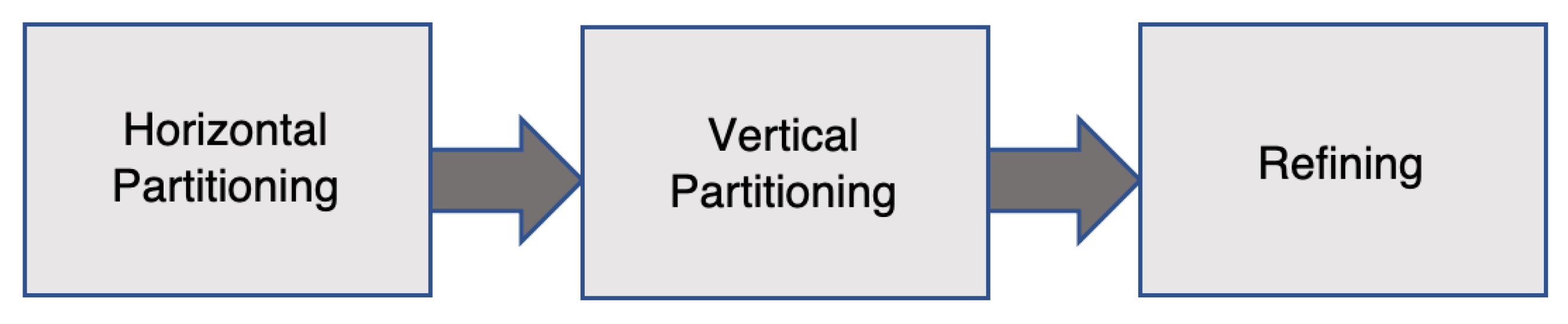
There are three steps involved in the process of dissociating transactions—first, horizontal partitioning groups transactions into clusters based on the most frequently occurring item. Then, vertical partitioning separates the items of a transaction into different columns to hide sensitive links between items. Lastly, the third stage improves the usefulness of the data by producing joint clusters (Figure 1).

• Horizontal partitioning
  The process of dissociation begins with the dividing of transactions into horizontal sections. During this stage, the transactions are partitioned into several groups that are referred to as clusters. In horizontal partitioning, a recursive approach is used to execute the binary partitioning of the transactions into groups according to the frequency of item occurrence in the dataset (Algorithm 1). In other words, the algorithm searches for the item that occurs the most frequently and then uses that information to categorise the transactions into two groups: the first group contains the transactions that include the item, and the second group includes the transactions that do not contain the item. After that, the algorithm searches for the next most frequent term for each group and splits the transactions again according to that. The process of partitioning will be carried out on each cluster of transactions until the clusters satisfy the desired size, which must be no less than k.
• Vertical partitioning
  After that, vertical partitioning will be implemented independently on each cluster resulting from the initial phase. The aim of vertical partitioning is to separate and hide unique combinations of items. Each cluster is divided vertically into two distinct types of columns, which are referred to as record chunks and a term chunk, respectively. The itemsets that fulfil the $k^m$-anonymity requirement are the ones that are included in record chunks. In a record chunk, each m-sized item combination must have a minimum of k occurrences. The items that accrue less than k times in a cluster are transferred into a different chunk called the term chunk. Each cluster may include many record chunks but but just a single term chunk.
  Consider the example in Table 4 as a demonstration of vertical partitioning. If $m=2$ and $k=2$, the transaction items are disassociated into the chunks given in Table 4, where all the resulting record chunks satisfy the $2^2$-anonymous requirement, and all the items that appear less than two times in the cluster are placed in the term chunk. In the third and fourth transactions, the combination of the Coronavirus and Pneumonia items is a $2^2$-anonymous sub-record. However, neither word appears frequently enough with Cough or Fatigue; thus, vertical partitioning moves them to another record chunk. In addition, the items that have not been included in the record chunks are transferred to a separate term chunk. Therefore, Migraine, Inflammation, Bronchitis and Asthma are placed in the term chunk (Table 4).
• Refining
  The refining stage aims to maximise the released information’s utility without sacrificing privacy. Therefore, this step attempts to reduce the total number of items in term chunks by including joint clusters for every two adjacent clusters. The reader is advised to see [37] for a more comprehensive explanation of the refining stage and the disassociation method.

Table 4. Disassociated transactions.

	Record Chunks		Term Chunk
ID	C1	C2	CT
1	Fatigue, Cough, Headache		Migraine
2	Fever, Cough, Headache	Coronavirus, Pneumonia	Inflammation
3	Fever, Fatigue, Headache	Coronavirus, Pneumonia	Bronchitis
4	Fever, Fatigue, Cough		Asthma

Table 4. Disassociated transactions.

	Record Chunks		Term Chunk
ID	C1	C2	CT
1	Fatigue, Cough, Headache		Migraine
2	Fever, Cough, Headache	Coronavirus, Pneumonia	Inflammation
3	Fever, Fatigue, Headache	Coronavirus, Pneumonia	Bronchitis
4	Fever, Fatigue, Cough		Asthma

Horizontal Partitioning Limitation

Using a recursive algorithm, horizontal partitioning accomplishes a binary dividing of data into groups determined by the number of times an item appears in the dataset. These groups are then divided further. The horizontal partitioning stage aims to ensure minimal data loss; ideally, each partitioned cluster will have a small number of transactions and a large number of associated items. As a consequence, the following stage, vertical partitioning, will involve less dissociation between the items, and the data will be more useful.

The original Algorithm 1 [13] first determines the most frequent term, and then that information is used to categorise the transactions into one of two categories: those that contain the item or those that do not include the item. The clusters are then segmented by the algorithm again based on the next most frequent item. For example, suppose k is equal to two, and we need to horizontally split the dataset in Table 1. In that case, the first iteration of the algorithm will choose the item Headache as the most common item in the dataset. The transactions will then be divided into two clusters using horizontal partitioning. The first cluster contains all the transactions that include the item Headache, while the second cluster has all the remaining transactions, as seen in

Table 5. Horizontal partitioning (the first iteration).

	Transactions
	Fatigue, Cough, Headache, Migraine
P1	Fever, Cough, Headache, Coronavirus, Pneumonia, Inflammation
	Fever, Fatigue, Headache, Coronavirus, Pneumonia, Bronchitis
P2	Fever, Fatigue, Cough, Asthma

.

Algorithm 1: HORPART.

The outcomes of the first round of horizontal partitioning are shown in Table 5 above. While $P1$ satisfies the size requirement, $P2$’s size is smaller than the k value. In consequence, this stage will abandon the division, and $P2$ and $P1$ will be recombined into a single cluster as a result of the horizontal partitioning stage (

Table 6. Horizontal partitioning (the resulting cluster).

	Transactions
P1	Fatigue, Cough, Headache, Migraine
	Fever, Cough, Headache, Coronavirus, Pneumonia, Inflammation
	Fever, Fatigue, Headache, Coronavirus, Pneumonia, Bronchitis
	Fever, Fatigue, Cough, Asthma

).

This stage focuses on minimising the splitting of items by creating independent groups of transactions where these groups have as few transactions and as many linked items in a cluster as possible. This will reduce the items’ disassociation and improve the data’s value. In contrast, skipping the partitioning process because one of the divided clusters is too small might result in massive clusters. For example, Table 6 demonstrates that there is no partitioning of the data and that all the transactions have returned to the same cluster. This might have an influence on how well the horizontal partitioning stage works.

5. Proposed Horizontal Partitioning Strategies

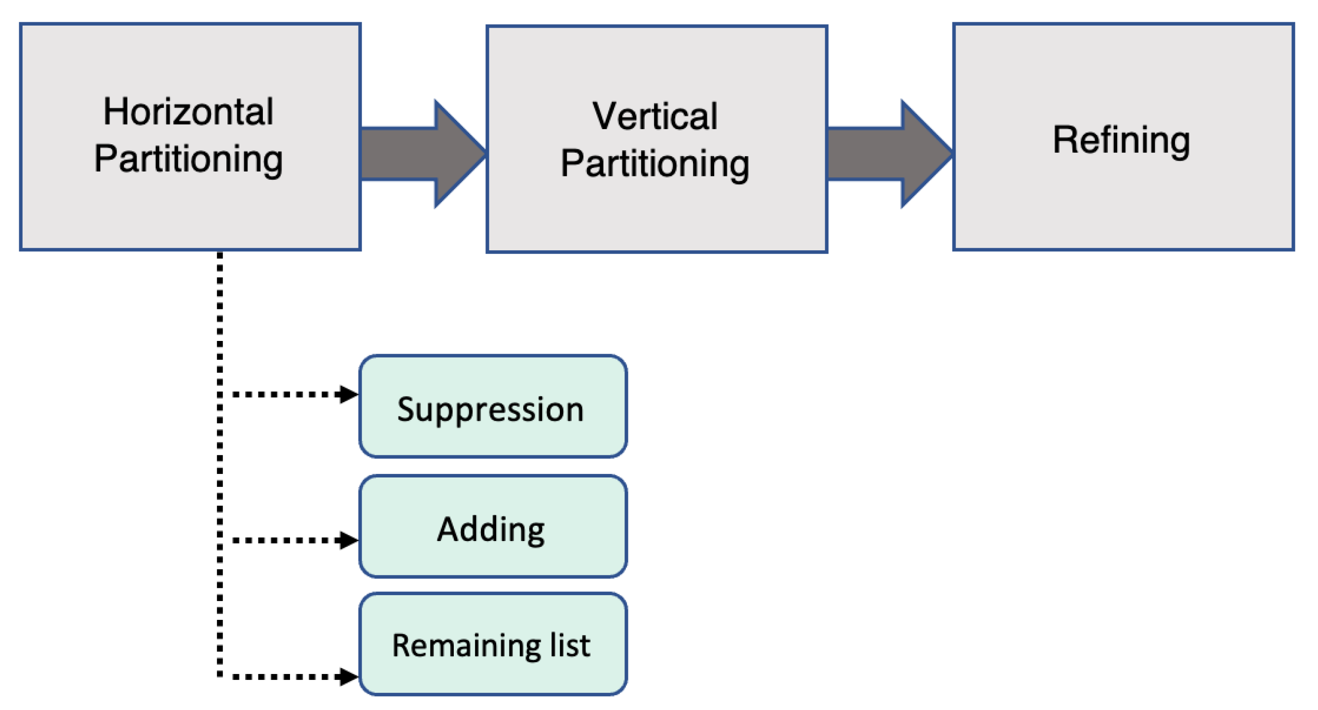
In order to solve the issue of cluster size in the original disassociation method, we introduce new algorithms and present an improved approach with three new strategies for dealing with cluster sizes of less than k (Figure 2). Our techniques improve upon original horizontal partitioning by including a verification stage. Two inputs are included in the checking step: the maximum cluster size and the k value. Whereas the k value will be used to establish the minimum allowable cluster size, the  maximum cluster size sets the greatest size of a cluster that does not necessitate additional partitioning. Three different cluster size scenarios must be considered in the horizontal partitioning stage (Figure 2):

• Based on our prior analysis, a dataset’s recursive partitioning into a cluster relies on two parameters, the maximum cluster size and k, to determine the partitioning’s termination condition. Therefore, the cluster will continue to be partitioned if its size is larger than the maximum cluster size.
• No additional partitioning is performed, and vertical partitioning will execute in the following step if the cluster size is between the maximum cluster size and the k value.
• In the case that the size of the cluster is less than the value of k, we will not abandon the horizontal partitioning process but rather implement one of the following strategies:

Figure 2. The improved disassociation method.

Figure 2. The improved disassociation method.

5.1. Suppression Strategy

According to this method, clusters with a size smaller than k are excluded from the published disassociated dataset. To dissociate transactions during the vertical partitioning stage, itemsets must occur in at least k transactions in order to meet the $k^m$-anonymity criterion. Therefore, in small clusters, all transaction terms will be moved to the term chunk because they do not occur frequently enough. This implies that certain transactions may not be advantageous for data analysis; hence, the approach will exclude them from the released data.

To illustrate our strategies, we extended the dataset presented in Table 1 as shown in

Table 7. Original transaction data (Extended Example).

TID	Original Transactions
1	Fatigue, Cough, Headache, Migraine
2	Fever, Cough, Headache, Coronavirus, Pneumonia, Inflammation
3	Fever, Fatigue, Headache, Coronavirus, Pneumonia, Bronchitis
4	Fever, Fatigue, Cough, Coronavirus, Pneumonia, Asthma
5	Glaucoma, Vision loss, Nausea, Trabeculectomy
6	Glaucoma, Vision loss, Nausea
7	Glaucoma, Vision loss, Headache
8	Glaucoma, Vision loss, Nausea, Vomiting
9	Glaucoma, Vision loss, Migraine
10	Stroke, Vision loss, Inflammation
11	Gastroenteritis, Bacteria, Pain
12	Gastroenteritis, Bacteria, nausea
13	Gastroenteritis, Bacteria, Pain
14	Bacteria, Pneumonia, Inflammation

. Assume we would like to publish the dataset in Table 7 as $2^2$ -anonymous and the maximum cluster size equals 3.

Algorithm 2 illustrates how the transaction suppression strategy functions. As a first step, the method examines a cluster’s size. To determine if a cluster is large enough, the algorithm compares its size to the maximum cluster size, then checks if it is more than or equal to k Line 4 and 5). If a cluster’s size is less than k, then it will be suppressed (Line 6). Otherwise, the method separates a cluster into two groups: one for records that do not include the most frequent term and another for all the other records that do contain the most frequent term (Lines 13 to 16). These procedures are performed iteratively for every cluster in the cluster queue Q until each cluster has an appropriate size. Terms that are already used in partitioning are preserved in the $ignore$ set and will not be reused for further splitting (Line 16).

Algorithm 2: Suppression method.

Firstly, we apply the first iteration of horizontal partitioning on the whole dataset to find the most common item, which is Vision loss (Lines 13 to 16). Then transactions are divided based on the most common item to $D_{!}$ and $D_2$ as shown in

Table 8. The first iteration of horizontal partitioning for Table 7.

	Transactions
$D_1$	Glaucoma, Vision loss, Nausea, Trabeculectomy
	Glaucoma, Vision loss, Nausea
	Glaucoma, Vision loss, Headache
	Glaucoma, Vision loss, Nausea, Vomiting
	Glaucoma, Vision loss, Migraine
	Stroke, Vision loss, Inflammation
$D_2$	Fatigue, Cough, Headache, Migraine
	Fever, Cough, Headache, Coronavirus, Pneumonia, Inflammation
	Fever, Fatigue, Headache, Coronavirus, Pneumonia, Bronchitis
	Fever, Fatigue, Cough, Asthma
	Gastroenteritis, Bacteria, Pain
	Gastroenteritis, Bacteria, nausea
	Gastroenteritis, Bacteria, Pain
	Bacteria, Pneumonia, Inflammation

.

In the second iteration of horizontal partitioning, the $D_1$ is divided again as its size is larger than the maximum cluster size (

Table 9. Horizontal partitioning for $D_1$ in Table 8 (suppression strategy).

(a) The second iteration for ${\mathit{D}}_1$
	Transactions
${D_1}_1$	Glaucoma, Vision loss, Nausea, Trabeculectomy
	Glaucoma, Vision loss, Nausea
	Glaucoma, Vision loss, Headache
	Glaucoma, Vision loss, Nausea, Vomiting
	Glaucoma, Vision loss, Migraine
${D_1}_2$	Stroke, Vision loss, Inflammation
(b) The third iteration for ${D_1}_1$
	Transactions
	Glaucoma, Vision loss, Nausea, Trabeculectomy
P1	Glaucoma, Vision loss, Nausea
	Glaucoma, Vision loss, Nausea, Vomiting
P2	Glaucoma, Vision loss, Headache
	Glaucoma, Vision loss, Migraine

). As a result, two new divisions will result from this step: ${D_1}_1$ and ${D_1}_2$. However, the size of ${D_1}_1$ is still larger than the maximum cluster size, so it will be divided again while ${D_1}_2$ is suppressed according to this strategy (Line 6). The third iteration of horizontal partitioning in Table 9a will produce two partitions with the allowable size for cluster formation so that they will be saved (Line 9). The same steps are applied on $D_2$ in Table 9 and the final clusters are illustrated in

Table 10. Horizontal partitioning for $D_2$ in Table 8 (suppression strategy).

(a) The second iteration for ${\mathit{D}}_2$
	Transactions
${D_2}_1$	Gastroenteritis, Bacteria, Pain
	Gastroenteritis, Bacteria, nausea
	Gastroenteritis, Bacteria, Pain
	Bacteria, Pneumonia, Inflammation
${D_2}_2$	Fatigue, Cough, Headache, Migraine
	Fever, Cough, Headache, Coronavirus, Pneumonia, Inflammation
	Fever, Fatigue, Headache, Coronavirus, Pneumonia, Bronchitis
	Fever, Fatigue, Cough, Asthma
(b) The third iteration for ${D_2}_1$
	Transactions
	Gastroenteritis, Bacteria, Pain
P1	Gastroenteritis, Bacteria, nausea
	Gastroenteritis, Bacteria, Pain
P2	Bacteria, Pneumonia, Inflammation
(c) The third iteration for ${D_2}_2$
	Transactions
	Fatigue, Cough, Headache, Migraine
P1	Fever, Fatigue, Headache, Coronavirus, Pneumonia, Bronchitis
	Fever, Fatigue, Cough, Asthma
P2	Fever, Cough, Headache, Coronavirus, Pneumonia, Inflammation

where $P_2$ in both Table 10b and Table 10c will be suppressed.

This strategy deals with a small cluster as a unique cluster, and transactions in this cluster need a high protection. Therefore, this strategy will not release small clusters into the published disassociated dataset. Although the data utility for this method can be low, it provides high protection for rare combinations in transactions. This could be an effective strategy for highly sensitive datasets (e.g., medical and financial transactions).

5.2. Adding Strategy

This strategy distributes small clusters among other clusters in the queue rather than suppressing them or abandoning the horizontal partitioning. This is because infrequent terms from one small cluster may be frequent in other, larger clusters. Hence, this method involves incorporating a number of smaller clusters into larger ones to increase the overall term frequency. Therefore, this strategy overcomes the issue caused by the original algorithm’s abandoning of partitioning.

The cluster size is checked in Algorithm 3 of the adding strategy, just as it is in the suppression strategy. No further partitioning of the cluster is executed if its size is less than or equal to the maximum cluster size and more than or equal to the k value (Line 14). This strategy will add the small cluster to the second cluster in the cluster queue Q if its size is less than k (Line 8). However, if there are no further clusters in the cluster queue, the small cluster will be added to the last saved cluster (Line 10). In order to horizontally partition a cluster, the algorithm searches for the most frequent term (Lines 18 to 20). These procedures are executed iteratively for each cluster in the cluster queue Q until all the clusters have an appropriate size. As a final step, the dataset’s horizontal partitioning is returned (Line 24).

Algorithm 3: Adding method.

If we used the same example in Table 7, the resulting divisions of the first iteration will be the same as in Table 8. For the second iteration of $D_1$ in the adding strategy, the transaction {Stroke, Vision loss, Inflammation} will be moved to the second cluster in Q, which will be $D_2$ (Line 8). Then $D_2$ will have a third iteration of horizontal partitioning. So, by using this strategy, we could find all transactions containing (Inflammation) as shown in

Table 11. Horizontal partitioning for $D_{2}2$ in Table 8 (adding strategy).

(a) The second iteration for ${\mathit{D}}_2$
	Transactions
${D_2}_1$	Gastroenteritis, Bacteria, Pain
	Gastroenteritis, Bacteria, nausea
	Gastroenteritis, Bacteria, Pain
	Bacteria, Pneumonia, Inflammation
${D_2}_2$	Fatigue, Cough, Headache, Migraine
	Fever, Cough, Headache, Coronavirus, Pneumonia, Inflammation
	Fever, Fatigue, Headache, Coronavirus, Pneumonia, Bronchitis
	Fever, Fatigue, Cough, Asthma
	Stroke, Vision loss, Inflammation
(b) The third iteration for ${D_2}_1$
	Transactions
	Gastroenteritis, Bacteria, Pain
P1	Gastroenteritis, Bacteria, nausea
	Gastroenteritis, Bacteria, Pain
P2	Bacteria, Pneumonia, Inflammation
(c) The third iteration for ${D_2}_2$
	Transactions
	Fatigue, Cough, Headache, Migraine
P1	Fever, Fatigue, Headache, Coronavirus, Pneumonia, Bronchitis
	Fever, Fatigue, Cough, Asthma
P2	Fever, Cough, Headache, Coronavirus, Pneumonia, Inflammation
	Stroke, Vision loss, Inflammation
	Bacteria, Pneumonia, Inflammation

c. This means increasing the frequency of this item and decreasing the number of items in the term chunks, which means better data utility.

This technique addresses the problem of dealing with small clusters by distributing them among other clusters that already exist. With this strategy, a cluster that is larger than the maximum cluster size will be sent back to the queue of clusters so that it can be divided horizontally once again. Therefore, if the division process produces a relatively small cluster, it will be added to the second cluster in the cluster queue Q. Consequently, this strategy will not delete any terms, thereby maintaining the utility of the data. In addition, it solves the issue of preventing the problem of producing large clusters.

5.3. Remaining List Strategy

This strategy deals with the issue of abandoning the horizontal partitioning by accumulating the resulting small clusters in another queue called the ’remaining list’. This technique involves verifying the size of each cluster and then adding those with sizes less than the k value to a separate list. When all the transactions have been horizontally partitioned, those in the remaining list will be treated as original transactions and moved to the main queue to apply the horizontal partitioning again. The process will be repeated until no more horizontal partitioning is possible.

Algorithm 4 shows how this strategy works. As a first step, the queue of the remaining list L will be created (Line 1). Then, while the size of L is larger than k, the two-step checking size will be applied to the transaction queue (Lines 4 and 5). If the size of the divided cluster is less than k, it will be moved to L. When this is not the case, the algorithm uses the most frequent term to split the large cluster in two (Lines 12 to 15). Once all the clusters in the cluster queue have been horizontally partitioned, the remaining list will be transferred to the cluster queue. If the size of the remaining list L is smaller than k, however, the transactions in the remaining list are added to the last cluster (Line 20).

Algorithm 4: Remaining list method.

Data: D, $MaxClusterSize$, k Result: D partitioned horizontally 1 $ignore\leftarrow \left\{\right\}$ , $Q\leftarrow D$, $L\leftarrow Q$ 2 while $L\ne \left\{\right\}$ do$\phantom{(}$ 3  if $L>k$ then 4   $\phantom{(}$$Q\leftarrow L$ $L\leftarrow \left\{\right\}$ 5   while $Q\ne \left\{\right\}$ do 6    $\phantom{(}$ {D}← head(Q) if$\left|D\right|<MaxClusterSize$ then 7     $\phantom{(}$if $\left|D\right|<k$ then 8      $\phantom{(}$$L\leftarrow L$ ∪ {D} 9     end$\phantom{(}$ 10     else$\phantom{(}$ 11      Save {D} 12     end$\phantom{(}$ 13     else$\phantom{(}$ 14      $T\leftarrow$ be the set of terms of D 15      Find the most frequent term x in (T − ignore) 16      $D1\leftarrow$ all records of D having term x 17      $D2\leftarrow D-D1$ 18     end$\phantom{(}$ 19    end$\phantom{(}$ 20   end$\phantom{(}$ 21   else$\phantom{(}$ 22    $TAIL\left(Q\right)\leftarrow tail\left(Q\right)$ ∪ L 23   end$\phantom{(}$ 24  end$\phantom{(}$ 25 end$\phantom{(}$ 26 return D partitioned horizontally

If we used the same example in Table 7, the resulting divisions of the first iteration will be the same as in Table 8. For the second iteration of $D_1$ and $D_2$ in this strategy, the transactions {Stroke, Vision loss, Inflammation} and {Fever, Cough, Headache, Coronavirus, Pneumonia, Inflammation} will be moved to the remaining list (Line 8). After ${D_2}_2$ have the third iteration of horizontal partitioning, the transaction {Bacteria, Pneumonia, Inflammation} will also be added to the remaining list. So by using the remaining list strategy, we could find all transactions containing (Inflammation), as shown in

Table 12. Horizontal partitioning for $D_2$ in Table 8 (remaining list strategy).

(a) The second iteration for ${\mathit{D}}_2$
	Transactions
${D_2}_1$	Gastroenteritis, Bacteria, Pain
	Gastroenteritis, Bacteria, nausea
	Gastroenteritis, Bacteria, Pain
	Bacteria, Pneumonia, Inflammation
${D_2}_2$	Fatigue, Cough, Headache, Migraine
	Fever, Cough, Headache, Coronavirus, Pneumonia, Inflammation
	Fever, Fatigue, Headache, Coronavirus, Pneumonia, Bronchitis
	Fever, Fatigue, Cough, Asthma
(b) The third iteration for ${D_2}_1$
	Transactions
	Gastroenteritis, Bacteria, Pain
P1	Gastroenteritis, Bacteria, nausea
	Gastroenteritis, Bacteria, Pain
P2	Bacteria, Pneumonia, Inflammation
	Remaining list
	Fever, Cough, Headache, Coronavirus, Pneumonia, Inflammation
	Stroke, Vision loss, Inflammation
(c) The third iteration for ${D_2}_2$
	Transactions
	Fatigue, Cough, Headache, Migraine
P1	Fever, Fatigue, Headache, Coronavirus, Pneumonia, Bronchitis
	Fever, Fatigue, Cough, Asthma
	Remaining list
	Fever, Cough, Headache, Coronavirus, Pneumonia, Inflammation
	Stroke, Vision loss, Inflammation
	Bacteria, Pneumonia, Inflammation

c, which will contribute to improving the data utility of the resulting disassociated transactions. However, the difference between the adding strategy and the remaining list strategy may not be distinctly noticeable in this example, as these strategies need a large number of transactions, making it difficult to include all of them in this paper.

This strategy allows low-frequency terms in a cluster to be identified more frequently by placing them in the remaining list and increasing the chance of finding the same terms in non-adjacent clusters.

6. Experiments

In this section, we undertake a series of experiments to evaluate the data utility of our proposed horizontal partitioning strategies versus the original horizontal algorithm.

6.1. Experimental Data and Setup

To conduct our experiments, we used three real transactional datasets that are introduced in [38]. First, the BMS-POS dataset is a transaction log from retail sales systems where each record reflects the items purchased by a single consumer during a single transaction. The two other datasets are BMS-WV1 and BMS-WV2, which contain several months of two e-commerce websites’ clickstream data. Each transaction in this data collection is represented as a web session that includes all the product detail pages looked at during that session. These datasets represent a benchmark in the data mining research community, as they are the most widely-used public transactional datasets.

Table 13. Experimental datasets.

Dataset	|D|	|T|	Maximum Transaction Size	Average Transaction Size
BMS-POS	515,597	1657	164	6.5
BMS-WV1	59,602	497	267	2.5
BMS-WV2	77,512	3340	161	5.0

illustrates the properties of these datasets.

The experiments were run on a MacOS with a 3.22 GHz 8-core CPU and an M1 processor, and Python was used as a programming language to execute these algorithms.

6.2. Measurements

Any anonymisation technique designed to preserve individuals’ privacy will result in the loss of information. However, this loss of information must be kept to a minimum in order to retain the ability to derive meaningful data from released data. Since disassociation protects data by hiding the sensitive links that form infrequent itemsets, the information loss is associated with itemsets that occurred in the original dataset but not in the disassociated dataset. Therefore, our proposed strategies attempt to control cluster size and prevent the production of clusters that are larger than the maximum cluster size because this will increase the cluster sizes, which may reduce the utility of the disassociated data.

We adopt $tlost$ measurement as an assessment measure to quantify the total amount of information loss due to the employment of the different horizontal partitioning strategies. The $tlost$ measure determines the fraction of itemsets that occurred at least k times in the original dataset D, but those itemsets are moved to term chunks in the disassociated dataset.

6.3. Results

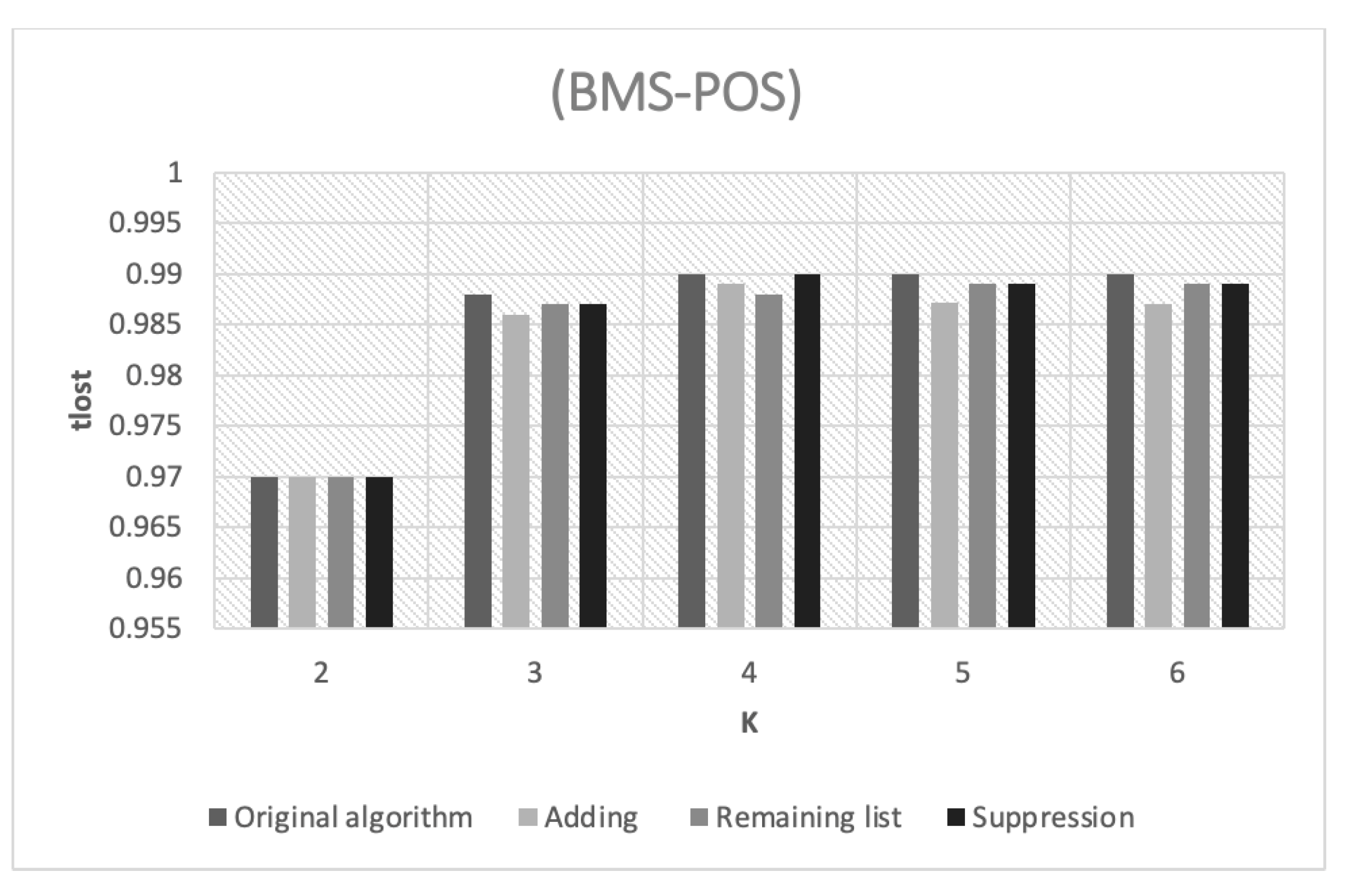
The amount of information loss in the POS dataset with varying k values is shown in Figure 3. However, even though the k values varied across the approaches, they all provide highly closed $tlost$ percentages, which might be interpreted as high percentages. This is due to the high density level, which means the frequency of items in this dataset is excessively high. Therefore, some clusters have a greater probability of transferring frequent itemsets to the term chunk.

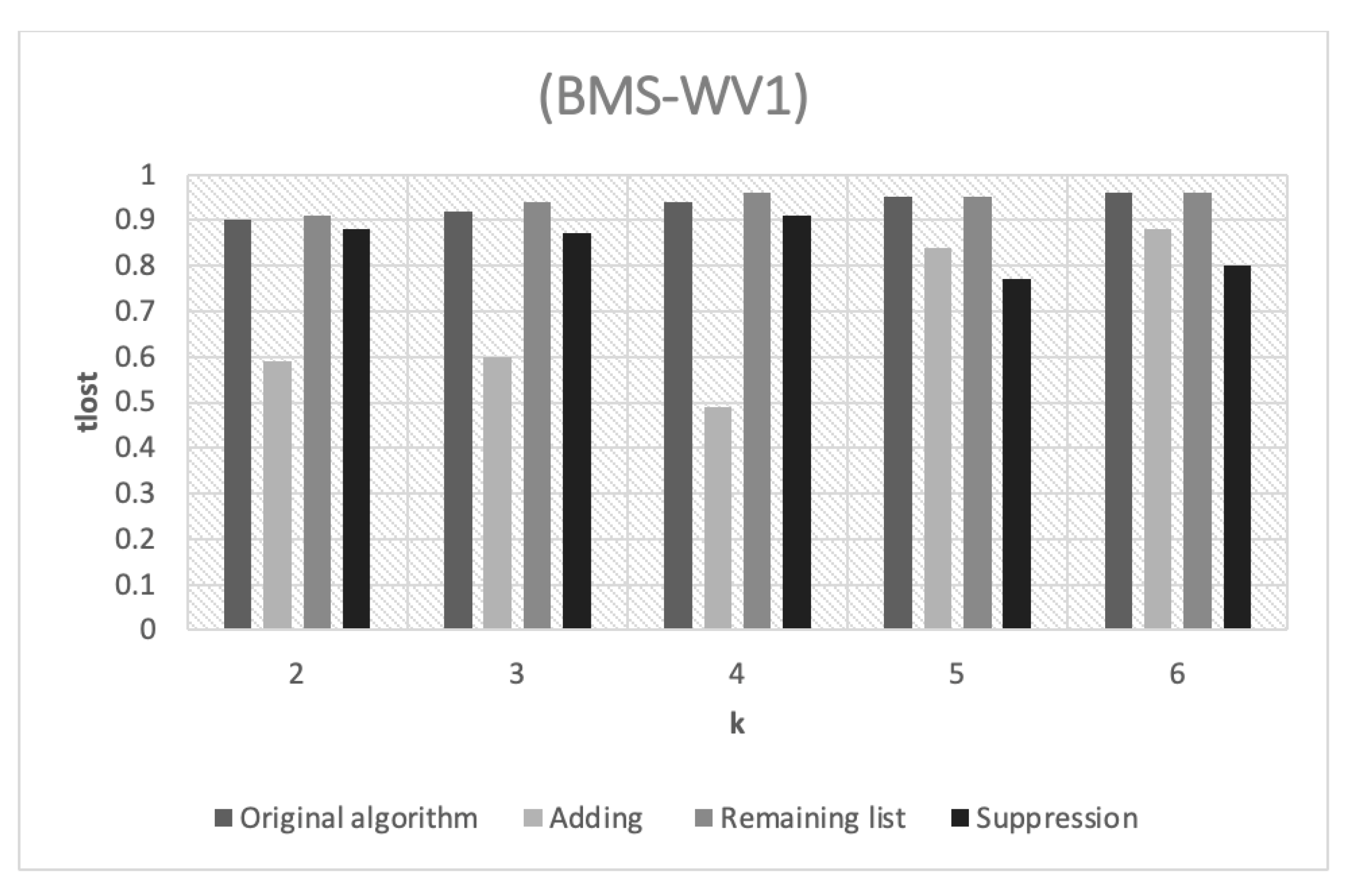
Figure 4 illustrates the amount of information loss in the WV1 dataset as a result of the various k values. The performance of the adding strategy is shown by the fact that it achieves the lowest $tlost$ percentages across all the k values. This is because the adding strategy depends on returning small clusters to the cluster queue by merging them with another big cluster. This merging allows the frequency of itemsets to be increased, which reduces the possibility of transferring these itemsets to term chunks, as is the case in the original horizontal partitioning algorithm. This explains the low information loss rates of this strategy.

However, the percentage of information loss for the remaining list strategy is relatively high compared to that of the adding strategy. This is because it relies on grouping the small clusters into one large cluster and then dividing it again. Consequently, the percentage of information loss depends on the probability of having similar itemsets in this remaining list. On the other hand, the suppression strategy has a low percentage of information loss due to the removal of small clusters from the disassociated dataset, which results in a modest proportion of information loss.

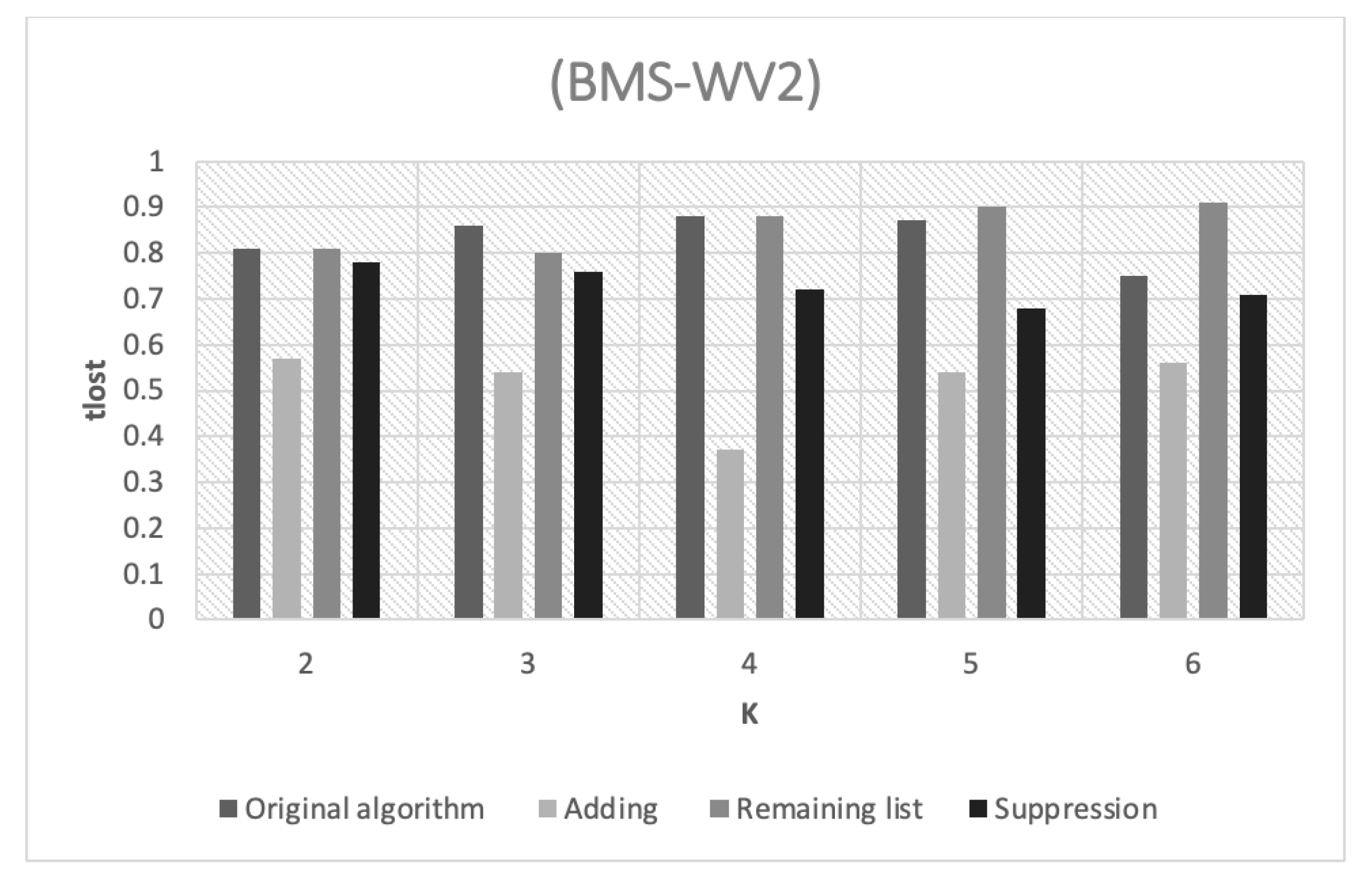
Figure 5 illustrates the amount of information loss in the WV2 dataset as a result of the various k values. In general, the performance levels of the different strategies are similar to the performance levels of the WV1 dataset. For example, the adding strategy still has the best information loss rates. However, the WV1 and WV2 datasets have a moderate density level, which results in more noticeable differences between the performance of the different horizontal partitioning strategies.

7. Conclusions and Future Work

In the original disassociation method, transactions are grouped into clusters using the k value. Therefore, the only requirement for approving the clusters produced by the horizontal partitioning phase is that neither cluster should be smaller than k. If not, this partitioning will be abandoned, and the original large cluster will be undivided. As a result, most items will be moved to term chunks, and data utilization will be impacted and fall below the actual level specified. This limitation of the disassociation method can impact the integrity of data analysis, resulting in inaccurate and unreliable findings. Due to the importance of accurate data analysis in the product development process, this problem may have far-reaching consequences for sustainable solutions. We addressed this issue by proposing three strategies for employing horizontal partitioning in our work—suppression, adding and remaining list—for dealing with clusters whose sizes are less than k. The addition strategy involves incorporating small clusters into existing larger ones, whereas the suppression strategy implies excluding them. In addition, small clusters in the remaining list technique will be moved to an external list; then, horizontal partitioning is applied to this list. Our proposed methods are designed to institute more stringent control over cluster sizes, which in turn improves data utilization. In addition, the proposed strategies provide greater flexibility by allowing data publishers to select the most appropriate strategy based on the degree of sensitivity of the data and the intended analysis purpose. However, our proposed strategies are intended to anonymise transactional data, so they are not designed to be used for other types of data, such as relational data.

In future work, we intend to expand our experiments to investigate the impact of changes in different properties and parameters, such as the data density, itemset size, and maximum cluster size. The other future work is investigating the possibility of data privacy breaches in our proposed improved disassociation algorithm.

References

- Tene, O.; Polonetsky, J. Big data for all: Privacy and user control in the age of analytics. Northwestern J. Technol. Intellect. Prop. 2012, 11, xxvii. [Google Scholar]
- Wu, X.; Zhang, S. Synthesizing high-frequency rules from different data sources. IEEE Trans. Knowl. Data Eng. 2003, 15, 353–367. [Google Scholar]
- Grossi, V.; Giannotti, F.; Pedreschi, D.; Manghi, P.; Pagano, P.; Assante, M. Data science: A game changer for science and innovation. Int. J. Data Sci. Anal. 2021, 11, 263–278. [Google Scholar] [CrossRef]
- Gangwar, H.; Mishra, R.; Kamble, S. Adoption of big data analytics practices for sustainability development in the e-commercesupply chain: A mixed-method study. Int. J. Qual. Reliab. Manag. 2023, 40, 965–989. [Google Scholar] [CrossRef]
- Li, N.; Li, T.; Venkatasubramanian, S. t-closeness: Privacy beyond k-anonymity and l-diversity. In Proceedings of the 2007 IEEE 23rd International Conference on Data Engineering, Istanbul, Turkey, 15–20 April 2007; pp. 106–115. [Google Scholar]
- Porter, C.C. De-identified data and third party data mining: The risk of re-identification of personal information. Shidler JL Com. Tech. 2008, 5, 1. [Google Scholar]
- He, Y.; Barman, S.; Naughton, J.F. Preventing equivalence attacks in updated, anonymized data. In Proceedings of the 2011 IEEE 27th International Conference on Data Engineering, Hannover, Germany, 11–16 April 2011; pp. 529–540. [Google Scholar]
- Zigomitros, A.; Solanas, A.; Patsakis, C. The role of inference in the anonymization of medical records. In Proceedings of the 2014 IEEE 27th International Symposium on Computer-Based Medical Systems, New York, NY, USA, 27–29 May 2014; pp. 88–93. [Google Scholar]
- Aïmeur, E.; Brassard, G.; Molins, P. Reconstructing profiles from information disseminated on the internet. In Proceedings of the 2012 International Conference on Privacy, Security, Risk and Trust and 2012 International Confernece on Social Computing, Amsterdam, The Netherlands, 3–5 September 2012; pp. 875–883. [Google Scholar]
- Frankowski, D.; Cosley, D.; Sen, S.; Terveen, L.; Riedl, J. You are what you say: Privacy risks of public mentions. In Proceedings of the 29th Annual International ACM SIGIR Conference on Research and Development in Information Retrieval, Seattle, WA, USA, 6–11 August 2006; pp. 565–572. [Google Scholar]
- Irani, D.; Webb, S.; Li, K.; Pu, C. Large online social footprints–an emerging threat. In Proceedings of the 2009 International Conference on Computational Science and Engineering, Vancouver, BC, Canada, 29–31 August 2009; Volume 3, pp. 271–276. [Google Scholar]
- Sweeney, L. k-anonymity: A model for protecting privacy. Int. J. Uncertain. Fuzziness Knowl.-Based Syst. 2002, 10, 557–570. [Google Scholar] [CrossRef]
- Loukides, G.; Liagouris, J.; Gkoulalas-Divanis, A.; Terrovitis, M. Disassociation for electronic health record privacy. J. Biomed. Inform. 2014, 50, 46–61. [Google Scholar] [CrossRef] [PubMed]
- Terrovitis, M.; Mamoulis, N.; Kalnis, P. Privacy-preserving anonymization of set-valued data. Proc. VLDB Endow. 2008, 1, 115–125. [Google Scholar] [CrossRef]
- Xu, Y.; Wang, K.; Fu, A.W.C.; Yu, P.S. Anonymizing transaction databases for publication. In Proceedings of the 14th ACM SIGKDD International Conference on Knowledge Discovery and Data Mining, Las Vegas, Ne, USA, 24–27 August 2008; pp. 767–775. [Google Scholar]
- Sweeney, L. Achieving k-anonymity privacy protection using generalization and suppression. Int. J. Uncertain. Fuzziness Knowl.-Based Syst. 2002, 10, 571–588. [Google Scholar] [CrossRef]
- Samarati, P.; Sweeney, L. Protecting Privacy When Disclosing Information: K-Anonymity and Its Enforcement through Generalization and Suppression. 1998. Available online: https://www.semanticscholar.org/paper/Protecting-privacy-when-disclosing-information%3A-and-Samarati-Sweeney/7df12c498fecedac4ab6034d3a8032a6d1366ca6 (accessed on 5 April 2023).
- Liu, J.; Wang, K. Anonymizing transaction data by integrating suppression and generalization. In Proceedings of the Pacific-Asia Conference on Knowledge Discovery and Data Mining, Hyderabad, India, 21–24 June 2010; Springer: Berlin/Heidelberg, Germany, 2010; pp. 171–180. [Google Scholar]
- Ruddell, B.L.; Cheng, D.; Fournier, E.D.; Pincetl, S.; Potter, C.; Rushforth, R. Guidance on the usability-privacy tradeoff for utility customer data aggregation. Util. Policy 2020, 67, 101106. [Google Scholar] [CrossRef]
- Yuvaraj, N.; Praghash, K.; Karthikeyan, T. Privacy preservation of the user data and properly balancing between privacy and utility. Int. J. Bus. Intell. Data Min. 2022, 20, 394–411. [Google Scholar] [CrossRef]
- Wondracek, G.; Holz, T.; Kirda, E.; Kruegel, C. A practical attack to de-anonymize social network users. In Proceedings of the 2010 IEEE Symposium on Security and Privacy, Oakland, CA, USA, 16–19 May 2010; pp. 223–238. [Google Scholar]
- Wang, K.; Xu, Y.; Fu, A.W.; Wong, R.C. ff-anonymity: When quasi-identifiers are missing. In Proceedings of the 2009 IEEE 25th International Conference on Data Engineering, Shanghai, China, 29 March–2 April 2009; pp. 1136–1139. [Google Scholar]
- Narayanan, A.; Shmatikov, V. How to break anonymity of the netflix prize dataset. arXiv 2006, arXiv:cs/0610105. [Google Scholar]
- Ciriani, V.; Capitani di Vimercati, S.D.; Foresti, S.; Samarati, P. κ-anonymity. In Secure Data Management in Decentralized Systems; Springer: Berlin/Heidelberg, Germany, 2007; pp. 323–353. [Google Scholar]
- Machanavajjhala, A.; Kifer, D.; Gehrke, J.; Venkitasubramaniam, M. L-diversity: Privacy beyond k-anonymity. ACM Trans. Knowl. Discov. Data (TKDD) 2007, 1, 3-es. [Google Scholar] [CrossRef]
- Navarro-Arribas, G.; Torra, V.; Erola, A.; Castellà-Roca, J. User k-anonymity for privacy preserving data mining of query logs. Inf. Process. Manag. 2012, 48, 476–487. [Google Scholar] [CrossRef]
- Park, H.; Shim, K. Approximate algorithms for k-anonymity. In Proceedings of the 2007 ACM SIGMOD International Conference on Management of Data, Beijing, China, 11–14 June 2007; pp. 67–78. [Google Scholar]
- He, Y.; Naughton, J.F. Anonymization of set-valued data via top-down, local generalization. Proc. VLDB Endow. 2009, 2, 934–945. [Google Scholar] [CrossRef]
- Wang, K.; Yu, P.S.; Chakraborty, S. Bottom-up generalization: A data mining solution to privacy protection. In Proceedings of the Fourth IEEE International Conference on Data Mining (ICDM’04), Brighton, UK, 1–4 November 2004; pp. 249–256. [Google Scholar]
- Iyengar, V.S. Transforming data to satisfy privacy constraints. In Proceedings of the Eighth ACM SIGKDD International Conference on Knowledge Discovery and Data Mining, Edmonton, AB, Canada, 23–26 July 2002; pp. 279–288. [Google Scholar]
- Xiao, X.; Tao, Y. Anatomy: Simple and effective privacy preservation. In Proceedings of the 32nd International Conference on Very Large Data Bases, Seoul, Republic of Korea, 12–15 September 2006; pp. 139–150. [Google Scholar]
- Chen, K.; Liu, L. Privacy preserving data classification with rotation perturbation. In Proceedings of the Fifth IEEE International Conference on Data Mining (ICDM’05), Houston, TX, USA, 27–30 November 2005; p. 4. [Google Scholar]
- Terrovitis, M.; Mamoulis, N.; Kalnis, P. Anonymity in unstructured data. In Proceedings of the International Conference on Very Large Data Bases (VLDB), Auckland, New Zealand, 23–28 August 2008. [Google Scholar]
- Loukides, G.; Gkoulalas-Divanis, A.; Malin, B. COAT: Constraint-based anonymization of transactions. Knowl. Inf. Syst. 2011, 28, 251–282. [Google Scholar] [CrossRef]
- Puri, V.; Sachdeva, S.; Kaur, P. Privacy preserving publication of relational and transaction data: Survey on the anonymization of patient data. Comput. Sci. Rev. 2019, 32, 45–61. [Google Scholar] [CrossRef]
- Puri, V.; Kaur, P.; Sachdeva, S. Effective removal of privacy breaches in disassociated transactional datasets. Arab. J. Sci. Eng. 2020, 45, 3257–3272. [Google Scholar] [CrossRef]
- Terrovitis, M.; Mamoulis, N.; Liagouris, J.; Skiadopoulos, S. Privacy preservation by disassociation. Proc. VLDB Endow. 2012, 5, 944–955. [Google Scholar] [CrossRef]
- Zheng, Z.; Kohavi, R.; Mason, L. Real world performance of association rule algorithms. In Proceedings of the Seventh ACM SIGKDD International Conference on Knowledge Discovery and Data Mining, San Francisco, CA, USA, 26–29 August 2001; pp. 401–406. [Google Scholar]