Seasonal Methods of Demand Forecasting in the Supply Chain as Support for the Company’s Sustainable Growth

Abstract

Demand forecasting plays a key role in supply chain planning, management and its sustainable development, but it is a challenging process as demand depends on numerous, often unidentified or unknown factors that are seasonal in nature. Another problem is limited availability of information. Specifically, companies lacking modern IT systems are constrained to rely on historical sales observation as their sole source of information. This paper employs and contrasts a selection of mathematical models for short-term demand forecasting for products whose sales are characterized by high seasonal variations and a development trend. The aim of this publication is to demonstrate that even when only limited empirical data is available, while other factors influencing demand are unknown, it is possible to identify a time series that describes the sales of a product characterized by strong seasonal fluctuations and a trend, using selected mathematical methods. This study uses the seasonal ARIMA (autoregressive integrated moving average) model, ARIMA with Fourier terms model, ETS (exponential smoothing) model, and TBATS (Trigonometric Exponential Smoothing State Space Model with Box–Cox transformation, ARMA errors, Trend and Seasonal component). The models are presented as an alternative to popular machine learning models, which are more complicated to interpret, while their effectiveness is often similar. The selected methods were presented using a case study. The results obtained were compared and the best solution was identified, while emphasizing that each of the methods used could improve demand forecasting in the supply chain.

1. Introduction

Demand forecasting is a critical component of a business’s operations and its ability to gain a competitive advantage in the market. Reliable and precise forecasts help businesses better adjust to market needs and meet customer demands more effectively [1,2]. In addition, they support process optimization, cost minimization, and reduce inventory problems [3,4,5]. Many companies, however, do not use mathematical forecasting at all, basing decisions on orders or inventory levels solely on subjective judgment or qualitative approaches [6,7,8,9].

One reason for this is the inherent difficulty of designing accurate forecasts. Demand is affected by numerous, often unidentified or unknown factors, such as seasonality, promotional effects, social events, new trends, unexpected crisis, terrorism, changes in weather conditions, commercial behavior of competitors in the market, etc. [1,4,5]. The problem lies both in the complexity of supply chains [10,11] and in the companies having limited access to information, often narrowed only to sales observations [1,12]. Data use is also limited due to different formats of archived data, lack of data integration tools, time of data collection, and timeliness of observations [13,14,15].

The need to reduce uncertainty in production, delivery planning, etc., means that organizations need methods to anticipate market needs in order to effectively manage all important aspects of the supply chain. This is why many researchers are looking into this issue. Modern demand forecasting methods using artificial intelligence and machine learning are the most popular nowadays [16].

One of the rapidly evolving trends in mathematical analysis involves the use of models that utilize big data [17,18]. In business management, the analysis of large data sets makes it possible to obtain more accurate forecasts that better reflect the needs of customers. It facilitates management, planning, as well as increases supply chain efficiency and reduces risk [19,20,21]. Current enterprise data-mining capabilities, the functioning Internet of Things, and other advances of the Fourth Industrial Revolution enable the collection of huge amounts of information [22]; hence, the rapid development of machine learning methods, while less and less attention is being paid to traditional analytical models [23,24,25]—which, as studies have shown—can prove to be more effective and justified for certain demand patterns [26].

The authors agree that both in the literature and in commercial systems (e.g., ERP) there is a steady increase in complex and complicated forecasting algorithms [26]. Meanwhile, the literature shows that often the data sets held by companies are too small relative to the expectations of models, such as neural networks, making it impossible to conduct tests or producing unreliable results [27,28]. The problem lies in the accuracy of demand forecasting models, especially in the case of significant distribution asymmetry [29], as well as the non-stationarity of the time series; neural network models perform better for stationary time series [30].

Based on the literature review, it seems that companies that are large in size, have a dominant position in the market, and a greater capacity for experimentation, are more prepared organizationally and receive greater support from top management for implementing information systems that allow the acquisition of accurate real-time data [31]. However, most companies lack such solutions and thus the ability to acquire accurate and precise information about the ongoing processes. It can take several years or even decades for them to achieve full IT integration [32]. It also turns out that many companies that have implemented IT systems fail to fully utilize their potential [33]. This is primarily because the dynamic development of such systems and the accompanying data analysis methods have become a perfect business opportunity. Numerous vendors offer advanced and sophisticated tools for data acquisition, storage, and forecasting, which, due to their complexity, are often not utilized [33]. Numerous studies show that, in such cases, forecasting is still done based on the knowledge and experience of managers, even despite obtaining unsatisfactory results [34,35].

This is due, according to many authors, to the use of very complex forecasting models. The authors emphasize that those responsible in companies for assessing future trends are often not econometricians and need simple, reliable information based on rational, understandable factors [36,37,38,39] so that the relationships between models, forecasts, and decisions are not complicated and are easily understood by decision-makers [38,39]. In general, cost savings are often recommended as one of the criteria for choosing between forecasting models [36], especially since many studies have shown that model complexity does not improve forecasting accuracy [38,40,41,42].

Nevertheless, model complexity is very popular among researchers and forecasters. The literature review indicates the greater prevalence of complex models, postulating even that researchers are rewarded for publishing in highly rated journals that favor the complexity of the solutions presented [37,38,39].

Meanwhile, the simplicity of forecasting encourages the use of such predictions and the abandonment of methods based solely on the knowledge and experience of experts.

It is also necessary to emphasize that many companies lack the ability to collect accurate data on the phenomenon under study, lack IT systems making it possible, and, consequently, can only rely on modest data on past sales [40], often lacking information on additional variables that could affect the sales being made [41]. The problem of access to the desired data is a significant challenge for many companies, especially small ones, and it is therefore necessary to present methods dedicated to such cases.

Furthermore, many entrepreneurs still prefer analytical time series models [1,11]. Moreover, the effectiveness of the developed learning algorithms is often ultimately compared with analytical ones anyway, which leads to the conclusion that the accuracy of deep learning methods is not statistically significantly better than that of regression [30,43], moving average [7,44], naive [45,46], autoregressive, as well as ARMA [47], ARIMA [9], SARIMA [47,48] models or the Poisson process [49,50]. Meanwhile, as the authors point out, analytical models are easier to configure and parameterize [45] and, above all, more readable in terms of interpreting individual parameters and assessing their impact on the dependent variable [51]. The authors also contend that the forecasting system should be stable [28], hence simpler forecasting methods and procedures are preferred to avoid issues with estimating and verifying the parameters.

This problem is pointed out by many authors in their search for effective methods. For example, in [51] the author points out the weakness of the statistical data held by companies, the inability to determine the distribution of the variable, and the use of inappropriate methods that do not reflect seasonality, especially in periods when demand reaches very low values. The problem with forecasting is also indicated by the authors in [28], pointing to the time-consuming nature of the forecasting process, its susceptibility to errors, and the noise that usually exists in such data, as well as its high dimensionality. That is why there is such a great need to verify and compare different forecasting methods in order to indicate the existing differences as well as the benefits of choosing specific models [27,28].

Accordingly, this paper responds to several problems identified in the literature and discussed above. As shown, advanced forecasting methods, especially those based on machine learning methods, are very popular in the literature, but they are inaccessible to many companies due to the inability to obtain accurate information in real time, as well as due to the difficulty in understanding and interpreting complex models. Therefore, the paper shows that simple analytical methods can also provide reliable forecasts, while increasing their sophistication does not clearly improve the results achieved. In addition, these methods can be used for simple time series concerning only past sales observations, without any additional factors—as in the cited example. Such methods are particularly useful for less developed companies. In addition, they are reproducible and thus easy to interpret, while being able to capture the most important relationships of the process under study. All the mathematical models proposed in the paper concern the analysis of seasonal data and allow for short-term forecasting of demand for products characterized by significant seasonal variations and a development trend. The literature review indicates the need for constructing such models, especially in situations of significant demand decline and irregular variations. This is particularly valuable for readers expecting specific guidelines on implementable solutions in their enterprises.

Seasonality of observations, limited availability of empirical data, and dynamic development of advanced forecasting methods therefore became the genesis of this paper. Its main purpose was to expose the existing problem, but primarily to verify selected forecasting methods applicable to seasonal demand on the basis of real data. Seasonality, as mentioned earlier, is one of the difficulties in forecasting demand, so the authors analyzed time series models specific to seasonal variations in observations.

The problems discussed and methods”prop’sed can inspire many companies and encourage the use of forecasting tools instead of the subjective opinion of experts.

On the other hand, the paper advocates the simplicity and usefulness of mathematical modeling and a discourse on the limitation of moving towards increasingly complex models.

At the same time, the presented solutions are an alternative to popular machine learning models, which are more complicated to interpret, while their effectiveness is often similar [52,53,54,55].

Thus, the adopted objectives of the research allowed the formulation of a hypothesis assuming that it is possible to forecast sales of products characterized by strong seasonal fluctuations and a trend in the supply chain by means of simple mathematical methods, and the indicated solutions can be implemented in any enterprise regardless of the level of its development and the level of computerization, since they require only simple time series of occurred observations.

The paper presents, after the Introduction, the methodology used in the research, then characterizes the subject of the research and collected observations, followed by a presentation of the mathematical models constructed. Finally, it presents their comparison, the selection of the best one and its detailed evaluation. The whole is concluded with a summary of the results obtained, conclusions, and indications of directions for further research.

2. Materials and Methods

The paper uses methods to identify time series with seasonal fluctuations. The seasonal ARIMA (autoregressive integrated moving average) model, ARIMA with Fourier terms model, ETS (exponential smoothing) model, and TBATS (Trigonometric Exponential Smoothing State Space Model with Box–Cox transformation, ARMA errors, Trend and Seasonal component) model were selected. A simple seasonal exponential smoothing model was used as a point of reference and comparison of the results obtained, as it enables assessment of the validity of constructing complex models. All calculations were performed using the R environment.

Selected time series models allow for short-term forecasting, as well as identification of the time series under study. Thus, they provide information on the demand for a given product and what can be expected in the near future. This information is more reliable compared to a subjective assessment based solely on the experience of managers, and, at the same time, obtained from the analysis of a simple time series. Such data is usually available in companies that lack advanced IT systems and do not use complex forecasting methods. In the paper, the difficulty of selected models is gradually increased to determine whether greater complexity results in better information, or whether simple models, such as the seasonal naive model discussed first below, are sufficient.

2.1. Seasonal Naive Model

Naive methods belong to the group of simple forecasting methods and are used for constructing short-term forecasts. They are most often used at a constant level of the phenomenon and small random fluctuations, but they can be extended to take into account seasonality, in which case the forecast at time $t+h$ is the last value of the observation in the corresponding period:

$$y_{t+h}=y_{t+h-m(k+1)}$$

(1)

where:

• $m$—seasonal period (number of cycle phases)
• $k$—the integer part of $\frac{h-1}{m}$

2.2. ARMA Class Models

Stationary models are popular among time series models. Depending on the time correlation structure, the following are distinguished [56,57,58,59]:

−

Autoregressive model of order $p$ AR($p$)

−

Moving Average model of order $q$ MA($q$)

Let $Y_t$ be a stationary time series.

The Moving Average model is the $y_t$ that satisfies the equation:

$$y_t={{\epsilon }_t-\beta }_1{\epsilon }_{t-1}-{\beta }_2{\epsilon }_{t-2}-{\dots -\beta }_q{\epsilon }_{t-q}$$

(2)

where ${\left\{{\epsilon }_t\right\}}_{t\in N}$ is a sequence of independent random variables with distribution $N(0,{\sigma }^2)$.

Such a series takes into account the existence of time correlation of the random component. Its strength and nature are determined by the parameter $q$—i.e., the order of the Moving Average model and individual model coefficients (${\beta }_q$).

The Autoregressive model is the series $y_t$ that satisfies the equation:

$$y_t={\alpha }_0+{\alpha }_1{y}_{t-1}+{\alpha }_2{y}_{t-2}+{\dots +\alpha }_p{y}_{t-p}+{\epsilon }_t$$

(3)

where ${\left\{{\epsilon }_t\right\}}_{t\in N}$ is a sequence of independent random variables with distribution $N\left(0,{\sigma }^2\right)$.

Such a series takes into account the existence of time correlation of the past realizations of the dependent variable. The value of the dependent variable at time $t$ is a linear combination of its time-lagged values and white noise interference.

By combining the AR and MA models, we obtain the ARMA time series of the form:

$$\begin{gathered} x_t={\alpha }_0+{\alpha }_1{y}_{t-1}+{\alpha }_2{y}_{t-2}+{\dots +\alpha }_p{\mathrm{y}}_{t-p}+{\epsilon }_t{\beta }_0+{{\epsilon }_t-\beta }_1{\epsilon }_{t-1}- \\ -{\beta }_2{\epsilon }_{t-2}-{\dots -\beta }_q{\epsilon }_{t-q} \end{gathered}$$

(4)

or its seasonal form ARMA $(P,Q{)}_s$.

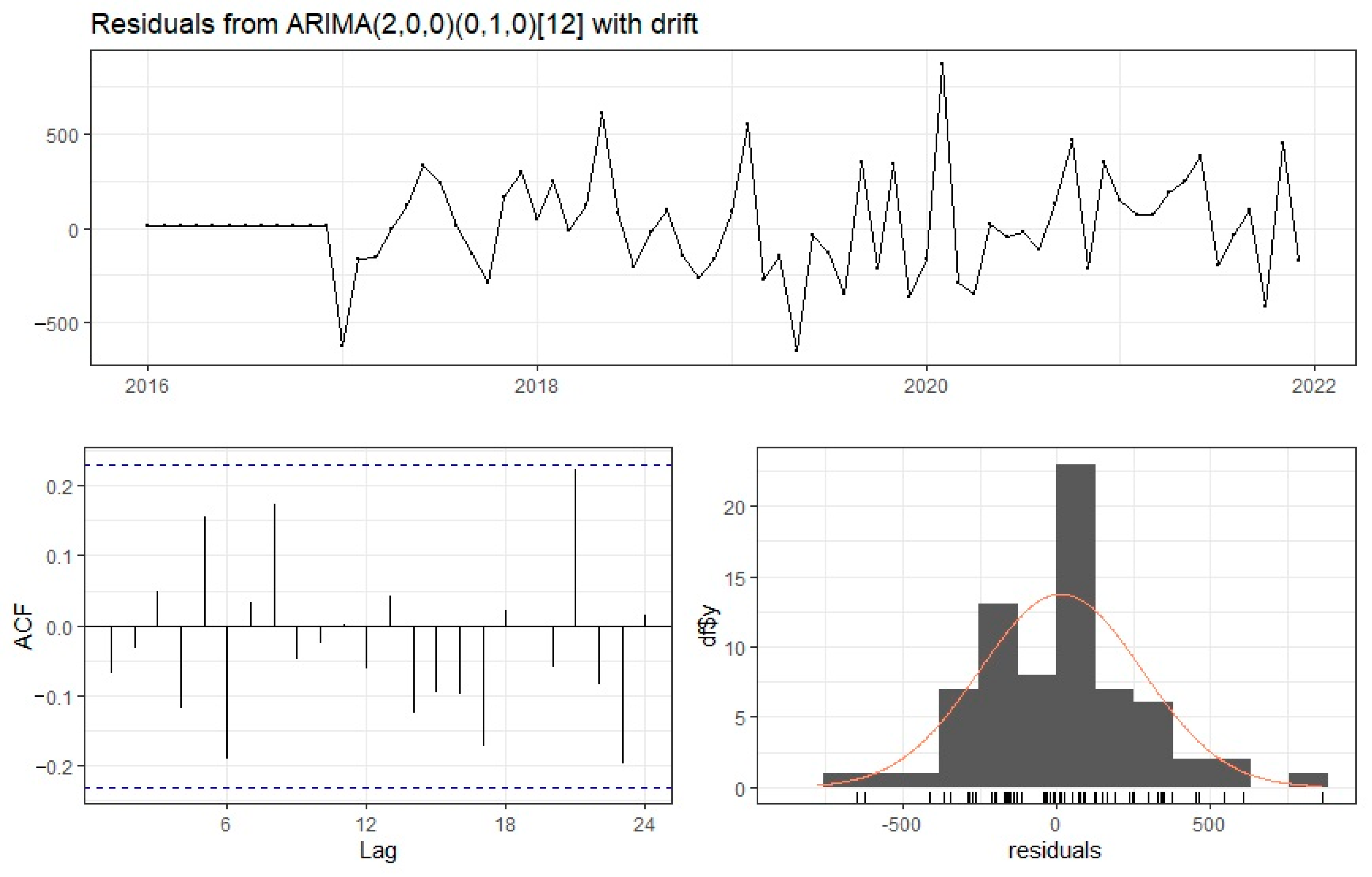
ARMA class models deal with stationary series. If this assumption is not met, transformations—e.g., differencing—are needed to obtain it. This results in the ARIMA (Autoregressive Integrated Moving Average) model and its seasonal version, SARIMA (Seasonal ARIMA). These are models that use a lagged differencing operation $d$.

2.3. ARIMA with Fourier Terms

ARIMA models regress the current value of data in a time series against its historical values, so they do not always deal with multiple seasonality. This allows the addition of external regressors [1]. In order to take seasonality into account in the time series under study, additional Fourier series were added to the ARIMA model.

$$y_t={\sum }_{i=1}^M{\sum }_{k=1}^{K_i}[\alpha \mathrm{s}\mathrm{i}\mathrm{n}(\frac{2\pi kt}{p_i})+\beta \mathrm{c}\mathrm{o}\mathrm{s}(\frac{2\pi kt}{p_i}\left)\right]+N_t$$

(5)

where $N_t$ is the ARIMA process.

• $M$—number of periods
• $\alpha ,\beta$—Fourier coefficients
• $K$—Maximum order(s) of Fourier terms
• value $K$ is selected by minimizing the AIC criterion

2.4. ETS Exponential Smoothing Models

The basic idea of exponential smoothing is to assign (exponentially) decreasing weights to historical observations when determining the forecast of a future observation. A general class of models, called ETS (exponential smoothing state space model), occupies a special place among the methods based on exponential smoothing. The individual letters of the acronym stand for error, trend, and seasonality, respectively. Its elements can be combined in an additive, multiplicative, or mixed way. The trend in exponential smoothing is a combination of two components—i.e., level $l$ and increment $b$ combined with each other, taking into account the damping parameter $\varphi \in \left[\mathrm{0,1}\right]$ in five possible ways. Denoting the trend forecast for $h$ subsequent periods as $T_h$, we obtain [49]:

• N—no trend (none) $T_h=l$
• A—Additive $T_h=l+bh$
• Ad—Additive damped $T_h=l+\left(\varphi +{\varphi }^2+\dots +{\varphi }^h\right)b$
• M—Multiplicative: $T_h$ = $l{b}^h$
• Md—Multiplicative damped: $T_h$ = $l{b}^{\left(\varphi +{\varphi }^2+\dots +{\varphi }^h\right)}$

Taking into account only the seasonal component (no seasonality, additive variant and multiplicative variant) and the trend, we obtain 15 exponential smoothing models. Additionally taking into account additive or multiplicative random disturbances, we obtain 30 different models, presented in

Table 1. Possible ETS models combinations.

ETS Models
ETS (M, M, N)	ETS (A, M, A)	ETS (M, N, M)
ETS (M, A, N)	ETS (A, Md, N)	ETS (M, N, A)
ETS (M, A, M)	ETS (A, Md, M)	ETS (M, N, N)
ETS (A, M, N)	ETS (A, N, A)	ETS (M, A, A)
ETS (A, N, N)	ETS (M, Ad, M)	ETS (A, Ad, M)
ETS (A, A, M)	ETS (M, Ad, N)	ETS (M, M, A)
ETS (M, M, M)	ETS (M, Md, M)	ETS (A, A, A)
ETS (A, N, M)	ETS (A, Ad, N)	ETS (A, Ad, A)
ETS (A, A, N)	ETS (M, Md, A)	ETS (M, Ad, A)
ETS (A, M, M)	ETS (M, Md, N)	ETS (A, Md, A)

[49].

The value optimizing the model form can be the minimization of the selected information criterion (AIC, AICC, BIC) or the forecast error (MSE, MAPE). In this paper, the models were compared using the Akaike Information Criterion (AIC).

Let $k$ denote the number of estimated parameters, and $L$ the maximum model reliability function. The AIC value is calculated from the formula:

$$\mathrm{AIC}=-2lnL+2k$$

(6)

The smaller the value of the Information Criterion, the better the model fit.

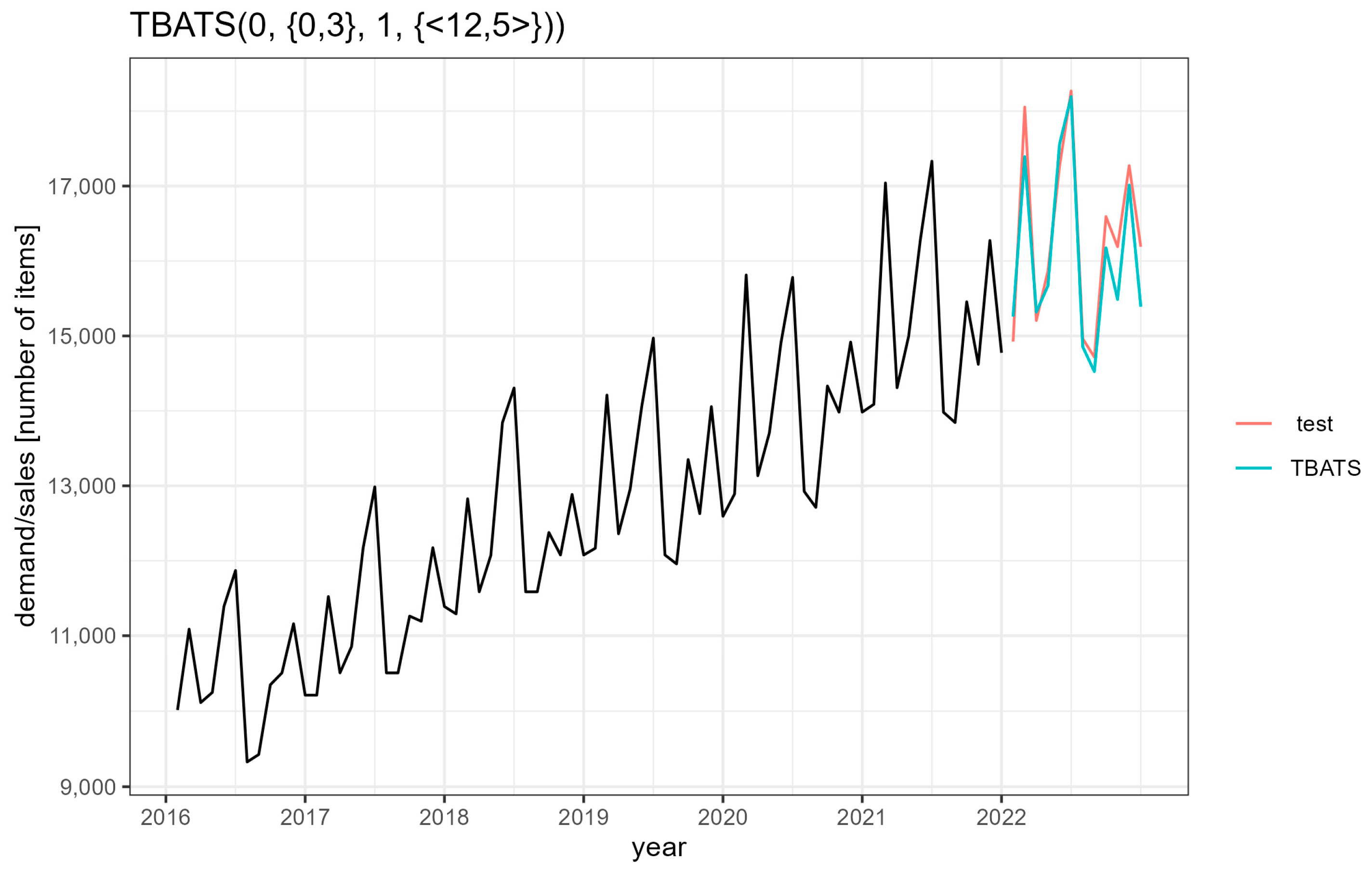
2.5. TBATS Model

The TBATS (Trigonometric Exponential Smoothing State Space model with Box–Cox transformation, ARMA errors, Trend and Seasonal component) model is a forecasting method for modeling non-stationary time series with complex seasonality using exponential smoothing. The structural form of the model is as follows:

$$\mathrm{TBATS}(\omega ,\mathrm{\Phi },p,q,\{m_1,k_1\},\{m_2,k_2\},\dots ,\{m_T,k_T\left\}\right)$$

(7)

where:

$\omega$—Box–Cox transformation parameter

$\varphi$—damping parameter

$p$ and $q$—number of AR and MA parameters

$m$—seasonal period

$k$—number of pairs of Fourier series

The model has the following form:

$$y_t^{\left(\omega \right)}=l_{t-1}+\phi b_{t-1}+{\sum }_{i=1}^T{s}_{t-1}^{\left(i\right)}+\alpha d_t$$

(8)

$$b_t=b_{t-1}+\beta d_t$$

$$s_t^{\left(i\right)}=\sum _{j=1}^{k_i}{s}_{j,t}^{\left(i\right)}$$

$$s_{j,t}^{\left(i\right)}=s_{j,t-1}^{\left(i\right)}cos{\lambda }_j^{\left(i\right)}+s_{j,t-1}^{\mathrm{*}}sin{\lambda }_j^{\left(i\right)}+{\gamma }_1^{\left(i\right)}{d}_t$$

$$s_{j,t}^{\mathrm{*}\left(i\right)}={-s}_{j,t-1}^{\left(i\right)}sin{\lambda }_j^{\left(i\right)}+s_{j,t-1}^{\mathrm{*}}cos{\lambda }_j^{\left(i\right)}+{\gamma }_2^{\left(i\right)}{d}_t$$

$${\lambda }_j^{\left(i\right)}=\frac{2\pi j}{m_i}$$

where:

• $i=1,\dots T$
• $d_t$—theoretical values of the ARMA $(p,q)$ model
• $\alpha ,\beta ,{\gamma }_1,{\gamma }_2—$smoothing parameters
• $l_t$—local level of the phenomenon under study over the period or at time $t$
• $b$—trend factor/value
• $s_{j,t}^{\left(i\right)}$—value of the seasonal component over the period $t$
• $m$—seasonal period

This method takes into account the Box–Cox transformation, seasonal variables and trend component, as well as autocorrelation of model residuals through the ARMA process.

The Box–Cox transformation is one of the transformations used in time series analysis to stabilize variance. It is also used as a transformation that transforms a continuous distribution of a random variable into a normal distribution (normalizing transformation).

We define the Box–Cox transformation as a transformation family of the form:

$$f_{\lambda }(y)=\left\{\begin{array}{c}\frac{y^{\lambda }-1}{\lambda },\lambda \ne 0\\ ln\left(y\right),\lambda =0\end{array},\right.$$

(9)

For $y>0$.

For $y_1, y_2, \dots , y_n$ time series, after applying the Box–Cox transformation, we obtain the series ${\tilde{y}}_1 = f_{\lambda }\left(y_1\right), {\tilde{y}}_2 = f_{\lambda }\left(y_2\right), \dots , {\tilde{y}}_n = f_{\lambda }\left(y_n\right)$.

The parameter $\lambda$ can take any real value. In practice, $\lambda =0$ (logarithmic transformation) or $\lambda = 1/2$ elemental transformation [60] are often used.

2.6. ADF Test

Unit root tests: the Augmented Dickey–Fuller test (ADF test) and the Kwiatkowski–Phillips–Schmidt–Shin test (KPSS test) [11,61] are most commonly used to test the stationarity of time series. In this paper, the ADF test is used to test for stationarity.

We represent the time series $\{y_t{\}}_{t\in N}$ as:

$$\Delta y_t=\theta y_{t-1}+{\sum }_{i=1}^k\Delta y_{t-i}+{\epsilon }_t$$

(10)

where ${\left\{{\epsilon }_t\right\}}_{t\in N}$ is a sequence of independent random variables with a normal distribution $N\left(0,{\sigma }^2\right)$.

The $k\in N$ order of autoregression should be selected to remove the correlations between the elements of the series ${\left\{{\epsilon }_t\right\}}_{t\in N}$. At the significance level of $0<\alpha <1$, we formulate a working hypothesis that the time series ${\left\{y_t\right\}}_{t\in N_0}$ is non-stationary (i.e., we assume $\theta =0$, therefore ${\left\{y_t\right\}}_{t\in N_0}\in I\left(d\right)$, and $d\ge 1$). As an alternative hypothesis, the time series ${\left\{y_t\right\}}_{t\in N_0}$ is assumed to be stationary (i.e., $\theta \in \left(-\mathrm{2,0}\right)$, therefore ${\left\{y_t\right\}}_{t\in N_0}\in I\left(0\right)$). The test statistic:

$$\mathrm{DF}=\frac{\widehat{\theta }}{S\left(\theta \right)}$$

(11)

is characterized by the Dickey–Fuller distribution, where $\widehat{\theta }$ is an estimator of the parameter $\theta$, while $S\left(\theta \right)$ is the standard deviation of this parameter. The value of the estimator of the parameter $\theta$ and the standard deviation are determined using the least squares method.

3. Demand Forecasting

3.1. Research Sample Characteristics

The company studied is engaged in the distribution of global brands of electronic equipment in Poland. The goods are imported from China. Observations on the sales of the company’s key product were studied. Observations are archived on a monthly basis. The collected data set was divided into a training set and a test set. The training set was used to construct models that identify the series under study and determine the forecast for the subsequent period. The test set was used to validate such models. The training set contains observations from January 2016 to December 2021 and the test set from January to December 2020. (Figure 1).

3.2. Seasonality Testing

Figure 1 shows a clear long-term trend; moreover, data are subject to seasonal variation, as confirmed by Figure 2.

Seasonal variations for most months are similar. There is a noticeable increase in the holiday months and in November, associated with pre-Christmas shopping in Europe, and a decrease at the turn of the year, caused by preparations and celebrations for the most important holiday in the traditional Chinese calendar—i.e., Chinese New Year falling between the end of January and the beginning of February.

3.3. Time Series Stationarity Testing

Construction of ARMA class models requires stationarity of the time series. The series under study is not stationary due to the presence of trend and seasonality. The occurrence and strength of the time correlation are shown in the graphs of the ACF and PACF functions (Figure 3 and Figure 4).

The graphs of autocorrelation and partial autocorrelation functions fade slowly, periodicity is evident, especially for a lag equal to 12 (annual seasonality). The result confirms the presence of a long-term trend and complex (multi-period) seasonality in the series.

The statistical non-stationarity of the series is confirmed by the results of the ADF test (

Table 2. ADF test results.

Type	No Drift No Trend		With Drift No Trend		With Drift and Trend
Lag	ADF	p-Value	ADF	p-Value	ADF	p-Value
0	−0.0653	0.623	−3.43	0.0151	8.27	0.01
1	0.2070	0.700	−2.39	0.1801	−8.18	0.01
2	0.8240	0.877	−1.43	0.5444	−5.39	0.01
3	1.2142	0.939	−1.03	0.6844	−4.53	0.01

).

Stationarity at the significance level of $\alpha =0.01$ was obtained after eliminating trend and drift in the series.

3.4. Naive Methods

Naive forecasting is the simplest method of estimating future values; hence, it is useful as a benchmark for other, more advanced time series identification and forecasting methods. Comparison with the naive method enables the evaluation of the effectiveness of more complex models, the use of which is justified by the fact that the sales phenomenon under study may be simultaneously subject to various fluctuations (of different periods). Due to the seasonality of the observations, the naive seasonal method was used. A graph of the forecast function according to the seasonal naive model and real observations is presented in Figure 5.

The forecast values are lower than the test observations. The model captures well the seasonality of the series only. It is less efficient in following the trend, underestimating the increase in the value of observations, which affects the forecast error results (

Table 3. Forecast error values for the seasonal naive model.

	ME	RMSE	MAE	MPE	MAPE
Test set	954.86	1010.53	954.86	7.20	7.20

).

3.5. ARIMA Model

The series under study were identified using the ARIMA model. The following seasonal model has been proposed: ARIMA (2,0,0) (0,1,0) [12] with drift. The parameters and evaluations of this model are shown in

Table 4. Parameters and evaluations of ARIMA (2,0,0) (0,1,0) [12] with the drift model.

		Estimate	Std. Error	z Value	Pr (>|z|)
ARIMA (2,0,0) (0,1,0) [12] with drift	ar1	0.2984	0.1253	2.3826	0.0172
	ar2	0.3184	0.1293	2.4624	0.0138
	drift	77.5370	7.8436	9.8854	$<2.2 \times {10}^{-16}$

.

All parameters of the model are statistically significant. The forecast errors are presented in

Table 5. Forecast errors for the ARIMA model.

		ME	RMSE	MAE	MPE	MAPE	MASE
ARIMA (2,0,0) (0,1,0) [12] with drift	Training set	13.2	262.57	189.52	0.02	1.43	0.2
	Test set	101.42	249.55	163.40	0.56	1.01	0.17

. Akaike’s criterion is 858.09.

The forecast effect according to the ARIMA model is presented in Figure 6.

It is evident that the ARIMA (1,1,1) (0,2,0) [12] model follows the series more closely, especially at times of low sales values.

3.6. ARIMA with Fourier Terms

In the ARIMA with Fourier terms model, seasonality is modeled by adding external regressors in the form of Fourier series. Their appropriate number was selected by estimating different models and minimizing the AIC. The ARIMA $(\mathrm{1,1},1)$ with a logarithmic Box–Cox transformation model was selected. The model parameters are shown in

Table 6. Regression with ARIMA (0,1,1) (1,0,0) [12] errors.

	Estimate	Std. Error	z Value	p Value
ma1	−0.7137	0.0989	−7.2132	$5.5 \times {10}^{-13}$
sar1	0.5602	0.1173	4.7735	$1.8 \times {10}^{-6}$
drift	73.3821	18.2517	4.0206	$5.8 \times {10}^{-5}$
S1-12	481.1897	88.8113	5.4181	$6 \times {10}^{-8}$
C1-12	−237.7423	87.3748	−2.7209	$6.5 \times {10}^{-3}$
S2-12	−359.9747	77.1620	−4.6652	$3.1 \times {10}^{-6}$
C2-12	317.8570	76.7958	4.1390	$3.4 \times {10}^{-5}$
S3-12	261.0701	74.7756	3.4914	$4.8 \times {10}^{-4}$
C3-12	−780.5381	74.8461	10.4286	$<2.2 \times {10}^{-16}$
S4-12	−579.8888	74.0158	−7.8347	$4.7 \times {10}^{-15}$
C4-12	131.8197	74.0979	1.7790	$7.5 \times {10}^{-2}$
S5-12	−402.5168	73.6940	−5.4620	$4.7 \times {10}^{-8}$
C5-12	230.7422	73.8928	−3.1227	$1.7 \times {10}^{-3}$

.

A graph of the forecast function according to the ARIMA (1,1,1) with the logarithmic Box–Cox transformation model and actual observations is presented in Figure 7.

The ARIMA with Fourier terms model captures the nature of only the first few test observations, while the fit to subsequent observations is negligible. When there is a clear increase in purchases, the model predicts a decrease. This leads to significant forecast errors, as presented in

Table 7. Regression with ARIMA (0,1,1) (1,0,0) [12] errors.

		ME	RMSE	MAE	MPE	MAPE	MASE
Regression with ARIMA (0,1,1) (1,0,0) [12] errors	Training set	9.70	268.60	210.38	0.03	1.65	0.22
	Test set	102.12	268.71	214.74	0.61	1.31	0.22

. Akaike’s criterion is 1029.93.

3.7. ETS

The parameters of various exponential smoothing models were estimated, and the optimal model variant was selected by minimizing the AIC and prediction errors. The selected model was ETS $(M,Ad,M)$, which takes into account multiplicative errors, additive damped trend, and multiplicative seasonality. The model has the following form [49]:

$$y_t=(l_{t-1}+\varphi b_{t-1})s_{t-1}^{(m-1)}(1+{\epsilon }_t)$$

$$l_t=(l_{t-1}+{\varphi b}_{t-1})(1+\alpha {\epsilon }_t)$$

$$b_t=\varphi b_{t-1}+\beta (l_{t-1}+{\varphi b}_{t-1}){\epsilon }_t$$

$$s_t^{\left(0\right)}=s_{t-1}^{(m-1)}(1+\gamma {\epsilon }_t)$$

$$s_t^{\left(i\right)}=s_{t-1}^{(i-1)},i=1,\dots ,m-1$$

The estimated parameters of this model are, respectively:

$$\alpha =0.0146$$

$$\beta =0.0001$$

$$\gamma =0.0001$$

$$\varphi =0.0215$$

A graph of the forecast function according to the ETS $(M,Ad,M)$ model and actual observations is presented in Figure 8.

The forecast errors are presented in

Table 8. Forecast errors for the ETS $(M,Ad,M)$ model.

		ME	RMSE	MAE	MPE	MAPE	MASE
$ETS(M,Ad,M)$	Training set	−14.7	241.9	182.8	−0.12	1.4	0.2
	Test set	285.6	366.2	285.6	1.7	1.7	0.3

.

3.8. TBATS Model

The structure of the TBATS model involves estimating and extracting the trend and seasonality component and determining a series of residuals for which a stationary model from the ARMA family is fitted. The extracted components of the studied time series are presented in Figure 9.

For the time series under study, a model of the following form was constructed:

TBATS (0, {0,3}, 1, {<12,5>}).

$$\mathrm{TBATS}(0,\{\mathrm{1,2}\},0.954,\{<\mathrm{12,5}>\left\}\right)$$

The value of the coefficient $\lambda$ of the Box–Cox transformation is $\lambda =6.5 \times {10}^{-5}$, which indicates a logarithmic transformation—i.e.:

$$Y=log\left(Y\right)$$

Three MA parameters of ${\beta }_1=0.1929$ and ${\beta }_2=0.4954 {\beta }_2=-0.3102$ were estimated, which means that in addition to the logarithmic transformation, it was necessary to additionally correct the theoretical values of the TBATS equations using the MA $\left(3\right)$ model.

The damping parameter Φ = 1 indicates a linear effect of the short-term trend from the previous period on the current value of the forecast variable.

The result of approximation by trigonometric Fourier series is 5 pairs of series with periodicity $m=12$.

The exponential smoothing parameters are:

$$\alpha =0.0674$$

$$\beta =0.0689$$

$${\gamma }_1=0.000006$$

$${\gamma }_2=0.00002$$

A graph of the forecast function according to the TBATS (0, {0,3}, 1, {<12,5>}) model and the actual observations is presented in Figure 10.

The graph of the forecast function accurately reflects the nature of the series of test observations, which indicates a good fit of the model to the empirical data.

The forecast errors are presented in

Table 9. Forecast errors for the $ETS(M,Ad,M)$ model.

		ME	RMSE	MAE	MPE	MAPE	MASE
$ETS(M,Ad,M)$	Training set	4.94	236.08	175.85	0.04	1.37	0.18
	Test set	285.60	366.20	285.60	1.70	1.70	0.30

.

Discussion of Results

The use of selected time series models dedicated to empirical data with a clear trend and seasonality against a simple time series on product sales is presented above. Simple mathematical models were chosen but graded in difficulty to show differences in forecast errors. The calculated forecast errors are shown in

Table 10. Forecast errors of the constructed models.

Model	AIC	ME	RMSE	MAE	MPE	MAPE	MASE
Naive		1043.20	1065.60	1043.20	6.40	6.40
TBATS	1134.10	223.10	420.35	346.86	1.33	2.11	0.36
ETS(MAdM)	1315.53	285.60	366.20	285.60	1.70	1.70	0.30
ARIMA (2,0,0) (0,1,0) [12] with drift	858.09	101.42	249.55	163.40	0.56	1.01	0.17
Regression with ARIMA (0,1,1) (1,0,0) [12] errors	1029.93	102.12	268.71	214.74	0.61	1.31	0.22

.

As can be seen, the differences in forecast errors are not drastic. In addition, Figure 5, Figure 6, Figure 7, Figure 8 and Figure 10 show that all models performed quite well in forecasting development trends and seasonal changes and can be used in short-term forecasting. The validity of the finally selected model still needs to be verified, of course, as presented below. Since the most satisfactory results were obtained for the ARIMA (2,0,0) (0,1,0) [12] with the drift model, the diagnostics are presented on this particular example, analyzing the distribution of residuals.

Stationarity analysis using the Box–Ljung test showed that at the significance level of $\alpha =0.05$, there are no grounds to reject the hypothesis of non-stationarity of the series. The value of the test statistic was X-squared = 0.35536, while $p\text{-}value=0.5511$; therefore, the series satisfies the condition of stationarity. A graph of the autocorrelation function is presented in Figure 11.

Normality of the distribution of residuals was confirmed by the Lilliefors test (D = 0.10705, p-value = 0.03995) at the significance level of α = 0.01.

The distribution of residuals from the ARIMA (2,0,0) (0,1,0) [12] with the drift model is presented in Figure 11.

The model, therefore, can be considered correct and usable for sales forecasting in companies. It can serve as an alternative to complex forecasting methods, and at the same time encourage the use of such considerations in companies where mathematical forecasting is not practiced. However, it should be emphasized that such models have limitations. They only utilize past information about the forecast variable and only demonstrate its change over time to construct a forecast. No additional factors that may also have a significant impact on the variable being studied—in this case, sales—are taken into account.

Nevertheless, in comparison to demand forecasting studies in the literature dominated by complex models and artificial intelligence methods, the obtained results show that it is possible to create easy-to-interpret and easy-to-use forecasts based solely on historical data of the studied phenomenon using mathematical models constructed for simple time series.

4. Conclusions

The market conditions in which companies operate are complex, characterized by intense competition and dynamic, often unpredictable transformations. To ensure success and continuity, businesses must be vigilant and quickly adapt to changes in their environment. Reliable forecasts, particularly in areas such as production management, inventory, distribution, or orders, can greatly assist in making key decisions within the supply chain.

It is undeniable that in sustainable supply chain management, the application of predictive models is of crucial importance, as such models enable companies to prepare in advance for future situations in order to meet customer demands and properly respond to the dynamics of market demand. Therefore, forecasting, even in the short-term, is a significant lever for improving supply chain performance and contributes to the sustainable business development in line with market needs and competition activity.

In the literature on demand forecasting, artificial intelligence is strongly emphasized as one of the key techniques used in Industry 4.0, along with other methods based on the Internet of Things and modern data acquisition technologies. This is facilitated by the dynamic development of companies, their computerization and digitization. However, there are also many small businesses that are less advanced, and even those that rely solely on managers’ experience rather than mathematical methods for forecasting. Such companies are the target audience for the analyses presented here, which have demonstrated that it is possible to create easy-to-interpret and easy-to-use forecasts based solely on historical data on the phenomenon being studied using simple time series.

Therefore, the aim of this study was to employ and contrast a selection of mathematical models for short-term demand forecasting for products whose sales are characterized by high seasonal variations and a development trend.

The mathematical models presented in this paper are a response to the possibility of making predictions using observations related to time series exhibiting seasonal fluctuations, which are characteristic of many products. The presented possibility of constructing a reliable forecast of sales volume is an excellent way to counteract the effects of seasonality, enabling the determination of the nature of the analyzed phenomenon, as well as forecasting its size within a specified time horizon.

Short-term forecasts play an important role in a company’s planning and management. Their accuracy contributes to cost reduction, process streamlining and increased customer satisfaction, which directly translates into profits and improves operational safety. This paper considers several models dedicated to data with clear seasonality. The seasonal ARIMA (autoregressive integrated moving average) model, ARIMA model with Fourier terms, ETS (exponential smoothing) model, and TBATS (Trigonometric Exponential smoothing state space model with Box–Cox transformation, ARMA errors, Trend and Seasonal component) model were selected. The results obtained were compared with the simple exponential smoothing model. It was noticed that all the presented models fulfilled the assumed postulates, and increasing their complexity did not significantly improve the calculated forecast errors. Therefore, a naive seasonal model may be sufficient for basic analysis.

This made it possible to verify the adopted hypothesis: it is possible to forecast the sales of products characterized by strong seasonal fluctuations and a trend using simple mathematical methods, while the proposed solutions can be implemented in any enterprise regardless of its level of development and level of computerization.

In further research, the presented methods will be developed using predictors other than past observations. The strong need for such research can be attributed to the fact that creating a forecast should be the first stage of planning the functioning strategy of each enterprise. Of course, the potential of innovative forecasting models should not be underestimated, but they should be adapted to the capabilities of the enterprise and specific applications. However, the principle of simplicity and ease of interpreting the results as well as usefulness for the enterprise should always be taken into account.

References

1. Loska, A.; Paszkowski, W. Geometric approach to machine exploitation efficiency: Modelling and assessment. Eksploat. I Niezawodn.–Maint. Reliab. 2022, 24, 114–122. [Google Scholar] [CrossRef]
2. Zabielska, A.; Jacyna, M.; Lasota, M.; Nehring, K. Evaluation of the efficiency of the delivery process in the technical object of transport infrastructure with the application of a simulation model. Eksploat. I Niezawodn.–Maint. Reliab. 2023, 25, 1. [Google Scholar] [CrossRef]
3. Abolghasemi, M.; Hurley, J.; Eshragh, A.; Fahimnia, B. Demand forecasting in the presence of systematic events: Cases in capturing sales promotions. Int. J. Prod. Econ. 2020, 230, 107892. [Google Scholar] [CrossRef]
4. Nia, A.R.; Awasthi, A.; Bhuiyan, N. Industry 4.0 and demand forecasting of the energy supply chain: A literature review. Comput. Ind. Eng. 2021, 154, 107128. [Google Scholar]
5. Rožanec, J.M.; Kažič, B.; Škrjanc, M.; Fortuna, B.; Mladenić, D. Automotive OEM demand forecasting: A comparative study of forecasting algorithms and strategies. Appl. Sci. 2021, 11, 6787. [Google Scholar] [CrossRef]
6. Izdebski, M.; Jacyna-Gołda, I.; Nivette, M.; Szczepański, E. Selection of a fleet of vehicles for tasks based on the statistical characteristics of their operational parameters. Eksploat. I Niezawodn.–Maint. Reliab. 2022, 24, 407–418. [Google Scholar] [CrossRef]
7. Kim, Y.; Kim, S. Forecasting charging demand of electric vehicles using time-series models. Energies 2021, 14, 1487. [Google Scholar] [CrossRef]
8. Spyridou, A. Evaluating Factors of Small and Medium Hospitality Enterprises Business Failure: A conceptual approach. Tour. Int. Multidiscip. J. Tour. 2019, 1, 25–36. [Google Scholar]
9. Yang, C.L.; Sutrisno, H. Short-Term Sales Forecast of Perishable Goods for Franchise Business. In Proceedings of the 2018 10th International Conference on Knowledge and Smart Technology (KST), Chiang Mai, Thailand, 31 January–3 February 2018; IEEE: Piscataway, NJ, USA, 2018; pp. 101–105. [Google Scholar]
10. Kantasa-Ard, A.; Nouiri, M.; Bekrar, A.; Ait el Cadi, A.; Sallez, Y. Machine learning for demand forecasting in the physical internet: A case study of agricultural products in Thailand. Int. J. Prod. Res. 2021, 59, 7491–7515. [Google Scholar] [CrossRef]
11. Kokoszka, P.; Young, G. KPSS test for functional time series. Statistics 2016, 50, 957–973. [Google Scholar] [CrossRef]
12. Rossetti, R. Forecasting the sales of console games for the Italian market. Econometrics 2019, 23, 76–88. [Google Scholar] [CrossRef] [Green Version]
13. Merkuryeva, G.; Valberga, A.; Smirnov, A. Demand forecasting in pharmaceutical supply chains: A case study. Procedia Comput. Sci. 2019, 149, 3–10. [Google Scholar] [CrossRef]
14. Musa, B.; Yimen, N.; Abba, S.I.; Adun, H.H.; Dagbasi, M. Multi-state load demand forecasting using hybridized support vector regression integrated with optimal design of off-grid energy Systems—A metaheuristic approach. Processes 2021, 9, 1166. [Google Scholar] [CrossRef]
15. Shu, Z.; Zhang, S.; Li, Y.; Chen, M. An anomaly detection method based on random convolutional kernel and isolation forest for equipment state monitoring. Eksploat. I Niezawodn.–Maint. Reliab. 2022, 24, 758–770. [Google Scholar] [CrossRef]
16. Liu, P.; Ming, W.; Hu, B. Sales forecasting in rapid market changes using a minimum description length neural network. Neural Comput. Appl. 2020, 33, 937–948. [Google Scholar] [CrossRef]
17. Florescu, A.; Barabas, S.A. Modeling and Simulation of a Flexible Manufacturing System—A Basic Component of Industry 4.0. Appl. Sci. 2020, 10, 8300. [Google Scholar] [CrossRef]
18. Wang, G.; Gunasekaran, A.; Ngai, E.W.T.; Papadopoulos, T. Big data analytics in logistics and supply chain management: Certain investigations for research and applications. Int. J. Prod. Econ. 2016, 176, 98–110. [Google Scholar] [CrossRef]
19. Iftikhar, R.; Khan, M.S. Social media big data analytics for demand forecasting: Development and case implementation of an innovative framework. In Research Anthology on Big Data Analytics, Architectures, and Applications; IGI Global: Hershey, PA, USA, 2022; pp. 902–920. [Google Scholar]
20. Seyedan, M.; Mafakheri, F. Predictive big data analytics for supply chain demand forecasting: Methods, applications, and research opportunities. J. Big Data 2020, 7, 53. [Google Scholar] [CrossRef]
21. Dong, T.; Yin, S.; Zhang, N. The Interaction Mechanism and Dynamic Evolution of Digital Green Innovation in the Integrated Green Building Supply Chain. Systems 2023, 11, 122. [Google Scholar] [CrossRef]
22. Yin, S.; Yu, Y. An adoption-implementation framework of digital green knowledge to improve the performance of digital green innovation practices for industry 5.0. J. Clean. Prod. 2022, 363, 132608. [Google Scholar] [CrossRef]
23. Evtodieva, T.E.; Chernova, D.V.; Ivanova, N.V.; Wirth, J. The internet of things: Possibilities of application in intelligent supply chain management. In Digital Transformation of the Economy: Challenges, Trends and New Opportunities; Springer: Cham, Switzerland, 2019; pp. 395–403. [Google Scholar]
24. Xu, T.; Han, G.; Qi, X.; Du, J.; Lin, C.; Shu, L. A hybrid machine learning model for demand prediction of edge-computing-based bike-sharing system using Internet of Things. IEEE Internet Things J. 2020, 7, 7345–7356. [Google Scholar] [CrossRef]
25. Mostafa, N.; Hamdy, W.; Alawady, H. Impacts of Internet of Things on Supply Chains: A Framework for Warehousing. Soc. Sci. 2019, 8, 84. [Google Scholar] [CrossRef] [Green Version]
26. Moroff, N.U.; Kurt, E.; Kamphues, J. Learning and statistics: A Study for assessing innovative demand forecasting models. Procedia Comput. Sci. 2021, 180, 40–49. [Google Scholar] [CrossRef]
27. Hui, X. Comparison and application of logistic regression and support vector machine in tax forecasting. In Proceedings of the 2020 International Signal Processing, Communications and Engineering Management Conference (ISPCEM), Montreal, QC, Canada, 27–29 November 2020; IEEE: Piscataway, NJ, USA, 2020. [Google Scholar]
28. Lei, H.; Cailan, H. Comparison of multiple machine learning models based on enterprise revenue forecasting. In Proceedings of the 2021 Asia-Pacific Conference on Communications Technology and Computer Science (ACCTCS), Shenyang, China, 22–24 January 2021; IEEE: Piscataway, NJ, USA, 2021; pp. 354–359. [Google Scholar]
29. Li, J.; Cui, T.; Yang, K.; Yuan, R.; He, L.; Li, M. Demand Forecasting of E-Commerce Enterprises Based on Horizontal Federated Learning from the Perspective of Sustainable Development. Sustainability 2021, 13, 13050. [Google Scholar] [CrossRef]
30. Poghosyan, A.; Harutyunyan, A.; Grigoryan, N.; Pang, C.; Oganesyan, G.; Ghazaryan, S.; Hovhannisyan, N. An Enterprise Time Series Forecasting System for Cloud Applications Using Transfer Learning. Sensors 2021, 21, 1590. [Google Scholar] [CrossRef]
31. Boumediene, R.; Kawalek, P.; Lorenzo, O. Predicting SMEs’ adoption of enterprise systems. J. Enterp. Inf. Manag. 2009, 22, 10–24. [Google Scholar] [CrossRef]
32. Markus, M.L.; Tanis, C. The enterprise systems experience-from adoption to success. In Framing the Domains of IT Research: Glimpsing the Future through the Past; Pinnaflex Educational Resources: Cincinnati, OH, USA, 2000; pp. 173–207. [Google Scholar]
33. Fildes, R.; Goodwin, P. Stability in the inefficient use of forecasting systems: A case study in a supply chain company. Int. J. Forecast. 2021, 37, 1031–1046. [Google Scholar] [CrossRef]
34. Petropoulos, F.; Kourentzes, N.; Nikolopoulos, K.; Siemsen, E. Judgmental selection of forecasting models. J. Oper. Manag. 2018, 60, 34–46. [Google Scholar] [CrossRef] [Green Version]
35. De Baets, S.; Harvey, N. Using judgment to select and adjust forecasts from statistical models. Eur. J. Oper. Res. 2020, 284, 882–895. [Google Scholar] [CrossRef]
36. Harvey, A.C. The Econometric Analysis of Time Series; Mit Press: Cambridge, MA, USA, 1990. [Google Scholar]
37. Branch, W.A.; Evans, G.W. A simple recursive forecasting model. Econ. Lett. 2006, 91, 158–166. [Google Scholar] [CrossRef] [Green Version]
38. Green, K.C.; Armstrong, J.S. Simple versus complex forecasting: The evidence. J. Bus. Res. 2015, 68, 1678–1685. [Google Scholar] [CrossRef] [Green Version]
39. Robin, M. Hogarth, Emre Soyer, Communicating forecasts: The simplicity of simulated experience. J. Bus. Res. 2015, 68, 1800–1809. [Google Scholar] [CrossRef]
40. Elliott, G.; Timmermann, A. Forecasting in economics and finance. Annu. Rev. Econ. 2016, 8, 81–110. [Google Scholar] [CrossRef] [Green Version]
41. Green, K.C.; Armstrong, J.S. Demand Forecasting: Evidence-Based Methods. Mark. Pap. 2012, 1–27. [Google Scholar] [CrossRef] [Green Version]
42. Wright, M.J.; Stern, P. Forecasting new product trial with analogous series. J. Bus. Res. 2015, 68, 1732–1738. [Google Scholar] [CrossRef] [Green Version]
43. Maaouane, M.; Zouggar, S.; Krajačić, G.; Zahboune, H. Modelling industry energy demand using multiple linear regression analysis based on consumed quantity of goods. Energy 2021, 225, 120270. [Google Scholar] [CrossRef]
44. Carbonneau, R.; Laframboise, K.; Vahidov, R. Application of machine learning techniques for supply chain demand forecasting. Eur. J. Oper. Res. 2008, 184, 1140–1154. [Google Scholar] [CrossRef]
45. Pacchin, E.; Gagliardi, F.; Alvisi, S.; Franchini, M. A comparison of short-term water demand forecasting models. Water Resour. Manag. 2019, 33, 1481–1497. [Google Scholar] [CrossRef]
46. Zhao, Y.; Ma, Z. Naïve Bayes-Based Transition Model for Short-Term Metro Passenger Flow Prediction under Planned Events. Transp. Res. Rec. 2022, 2676, 03611981221086645. [Google Scholar] [CrossRef]
47. Al-Saba, T.; El-Amin, I. Artificial neural networks as applied to long-term demand forecasting. Artif. Intell. Eng. 1999, 13, 189–197. [Google Scholar] [CrossRef]
48. Divisekara, R.W.; Jayasinghe, G.J.M.S.R.; Kumari, K.W.S.N. Forecasting the red lentils commodity market price using SARIMA models. SN Bus. Econ. 2021, 1, 20. [Google Scholar] [CrossRef]
49. Hyndman, R.; Koehler, A.B.; Ord, J.K.; Snyder, R.D. Forecasting with Exponential Smoothing: The State Space Approach; Springer Science & Business Media: New York, NY, USA, 2008. [Google Scholar]
50. Lee, H.; Lee, T. Demand modelling for emergency medical service system with multiple casualties cases: K-inflated mixture regression model. Flex. Serv. Manuf. J. 2021, 33, 1090–1115. [Google Scholar] [CrossRef]
51. Doszyń, M. Intermittent demand forecasting in the Enterprise: Empirical verification. J. Forecast. 2019, 38, 459–469. [Google Scholar] [CrossRef]
52. Smith, B.L.; Williams, B.M.; Oswald, R.K. Comparison of parametric and nonparametric models for traffic flow forecasting. Transp. Res. Part C Emerg. Technol. 2002, 10, 303–321. [Google Scholar] [CrossRef]
53. Katris, C. Prediction of unemployment rates with time series and machine learning techniques. Comput. Econ. 2020, 55, 673–706. [Google Scholar] [CrossRef]
54. Nan, H.; Li, H.; Song, Z. An adaptive PC-Kriging method for time-variant structural reliability analysis. Eksploat. I Niezawodn.–Maint. Reliab. 2022, 24, 532–543. [Google Scholar] [CrossRef]
55. Cerqueira, V.; Torgo, L.; Soares, C. Machine learning vs statistical methods for time series forecasting: Size matters. arXiv 2019, arXiv:1909.13316. [Google Scholar]
56. Borucka, A. Risk analysis of accidents in Poland based on ARIMA model. In Proceedings of the 22nd International Scientific Conference. Transport Means 2018, Trakai, Lithuania, 3–5 October 2018; pp. 162–166. [Google Scholar]
57. Jadevicius, A.; Huston, S. ARIMA modelling of Lithuanian house price index. Int. J. Hous. Mark. Anal. 2015, 8, 135–147. [Google Scholar] [CrossRef]
58. Song, Y.; Cao, J. An ARIMA-based study of bibliometric index prediction. Aslib J. Inf. Manag. 2022, 74, 94–109. [Google Scholar] [CrossRef]
59. Borucka, A.; Kozłowski, E.; Oleszczuk, P.; Świderski, A. Predictive analysis of the impact of the time of day on road accidents in Poland. Open Eng. 2020, 11, 142–150. [Google Scholar] [CrossRef]
60. Box, G.E.P.; Cox, D.R. An analysis of transformations. J. R. Stat. Soc. B 1964, 26, 211–252. [Google Scholar] [CrossRef]
61. Jaroń, A.; Borucka, A.; Parczewski, R. Analysis of the Impact of the COVID-19 Pandemic on the Value of CO2 Emissions from Electricity Generation. Energies 2022, 15, 4514. [Google Scholar] [CrossRef]
Figure 1. Product sales between 2016 and 2022, split into training and test sample.
Sustainability 15 07399 g001
Figure 2. Seasonality chart.
Sustainability 15 07399 g002
Figure 3. Graph of the autocorrelation function.
Sustainability 15 07399 g003
Figure 4. Graph of the partial autocorrelation function.
Sustainability 15 07399 g004
Figure 5. Graph of the forecast function according to the naive model.
Sustainability 15 07399 g005
Figure 6. Graph of the forecast function according to ARIMA model.
Sustainability 15 07399 g006
Figure 7. Graph of the forecast function according to the ARIMA (1,1,1) with regressors model.
Sustainability 15 07399 g007
Figure 8. Graph of the forecast function according to the ETS ( M , A d , M ) model.
Sustainability 15 07399 g008
Figure 9. Decomposition of the time series.
Sustainability 15 07399 g009
Figure 10. Graph of the forecast function according to the TBATS (0, {0,3}, 1, {<12,5>}) model.
Sustainability 15 07399 g010
Figure 11. Analysis of the distribution of residuals from the ARIMA (2,0,0) (0,1,0) [12] with the drift model.
Sustainability 15 07399 g011