
A Short-Term Parking Demand Prediction Framework Integrating Overall and Internal Information


Abstract
1. Introduction
- A multi-parking prediction model combining the whole and local aspects is constructed by combining two aspects: the whole block and its interior. Compared with the traditional multi-parking prediction task, the approach splits and transforms the pure point prediction task and is able to capture more factors associated with it. Thus, the accuracy of parking demand prediction improves by using the more factors.
- For the prediction model, a combination of GCN and GRU is chosen to effectively extract temporal and spatial information from the data. The model is based on historical parking demand data, and while using encoder–decoder to extract the characteristics of demand itself. It also fuses the temporal and spatial factors that have an impact on the parking demand of road sections. The combination of such multiple neural network layers obtains the required information in a complex urban road network. Thus, it fuses multiple sources of data effectively and obtains more desirable prediction results.
- A variety of features and influencing factors related to parking demand are analyzed. In addition to considering some inherent external factors, such as weather and holidays, improved spatial class features are also added. The features use more detailed representation methods, such as representing the spatial distance relationship between road sections using their driving times, and representing their semantic functions using the number and distance of various types of points of interest around the road sections, etc. At the same time, these analyzed features are also divided and incorporated into the model from both overall and local perspectives to enrich the influencing factors from the input perspective as meticulously as possible.
- The validation is performed using a real parking dataset from Xiufeng District of Guilin. The good performance of the model in this paper is reflected from the validation results, especially this structure of combining the whole block with the block interior. In addition, the robustness of the model is also reflected by using such a dataset with general accuracy. Finally, the design of the ablation experiment and the comparison of the results demonstrate the importance of considering each feature in the model.
2. Related Work
2.1. Parking Demand Prediction Based on Static Traffic
2.2. Parking Demand Prediction Based on Machine Learning
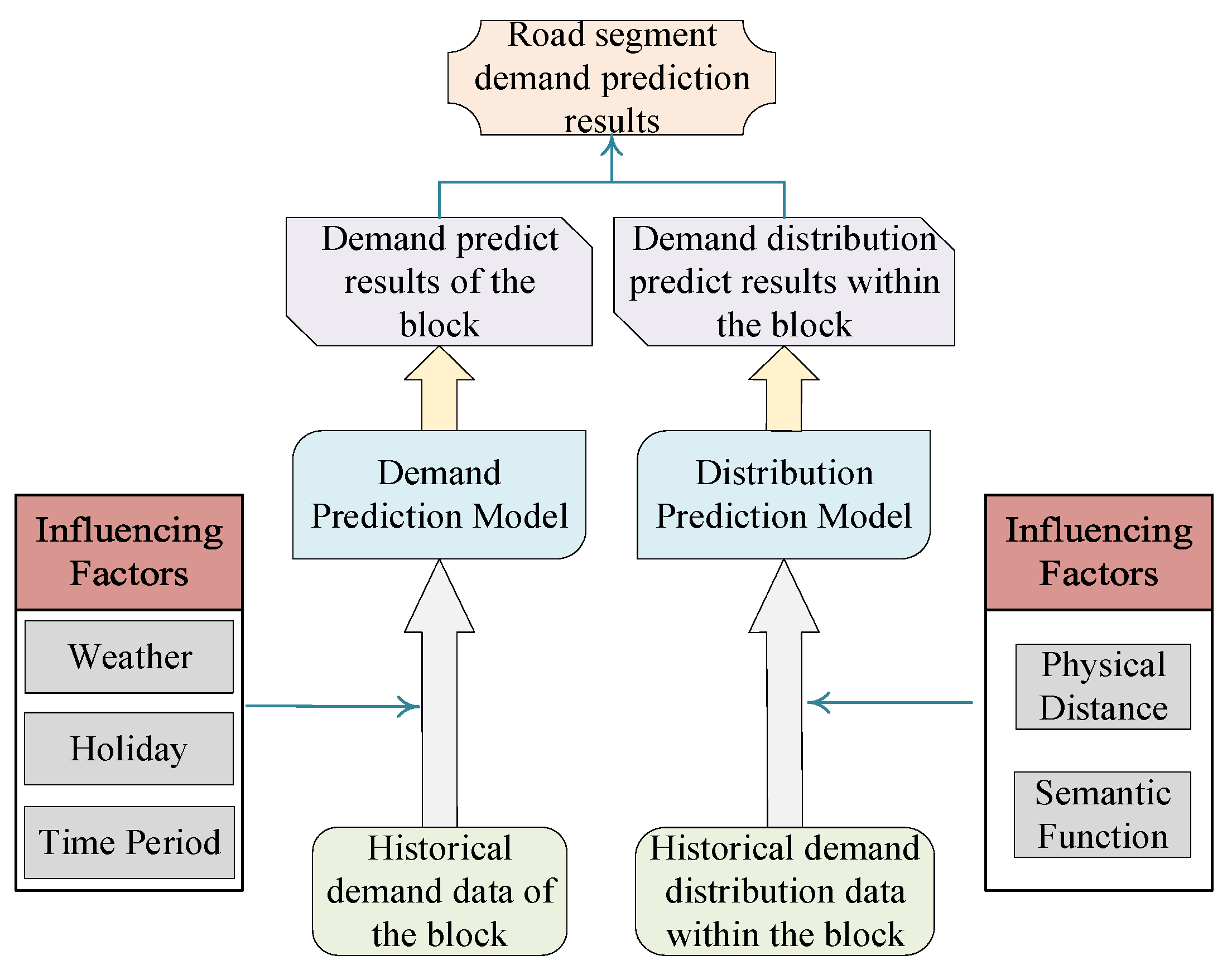
3. Materials and Methods
3.1. Preliminary
- (1)
- Overall Parking Demand Prediction of Block
- (2)
- Parking Demand Distribution Prediction within Block
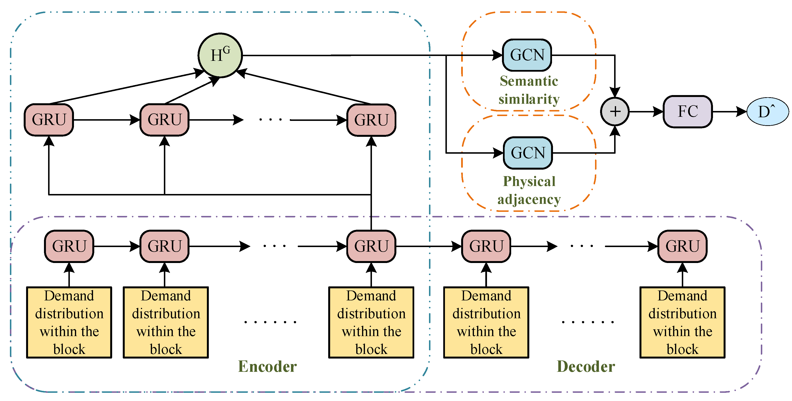
3.2. Parking Demand Prediction of Road Sections
3.2.1. Overall Parking Demand Prediction of Block
Feature Analysis
- (1)
- Weather
- (2)
- Holiday Events
- (3)
- Time Factors
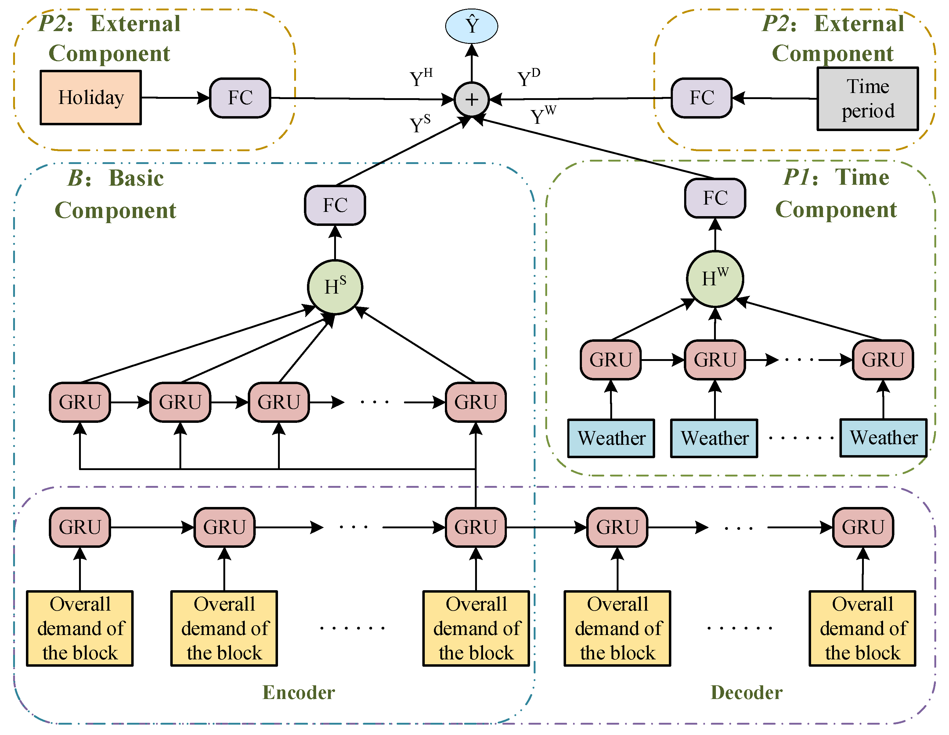
Model Design
3.2.2. Parking Demand Distribution Prediction within Block
Feature Analysis
- (1)
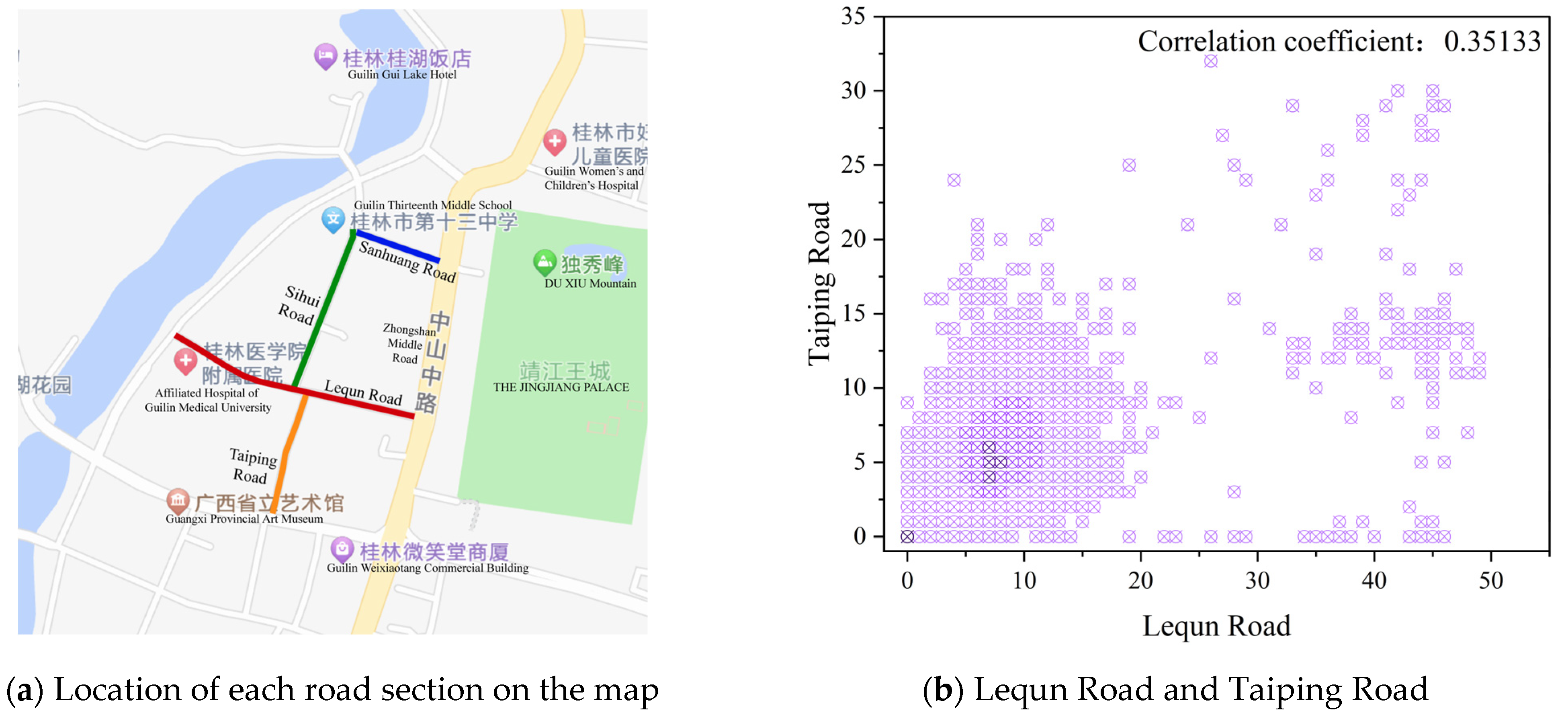
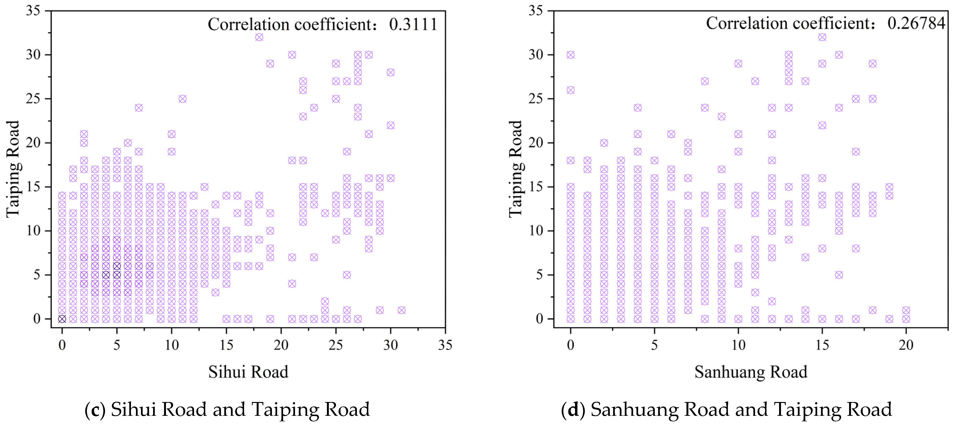
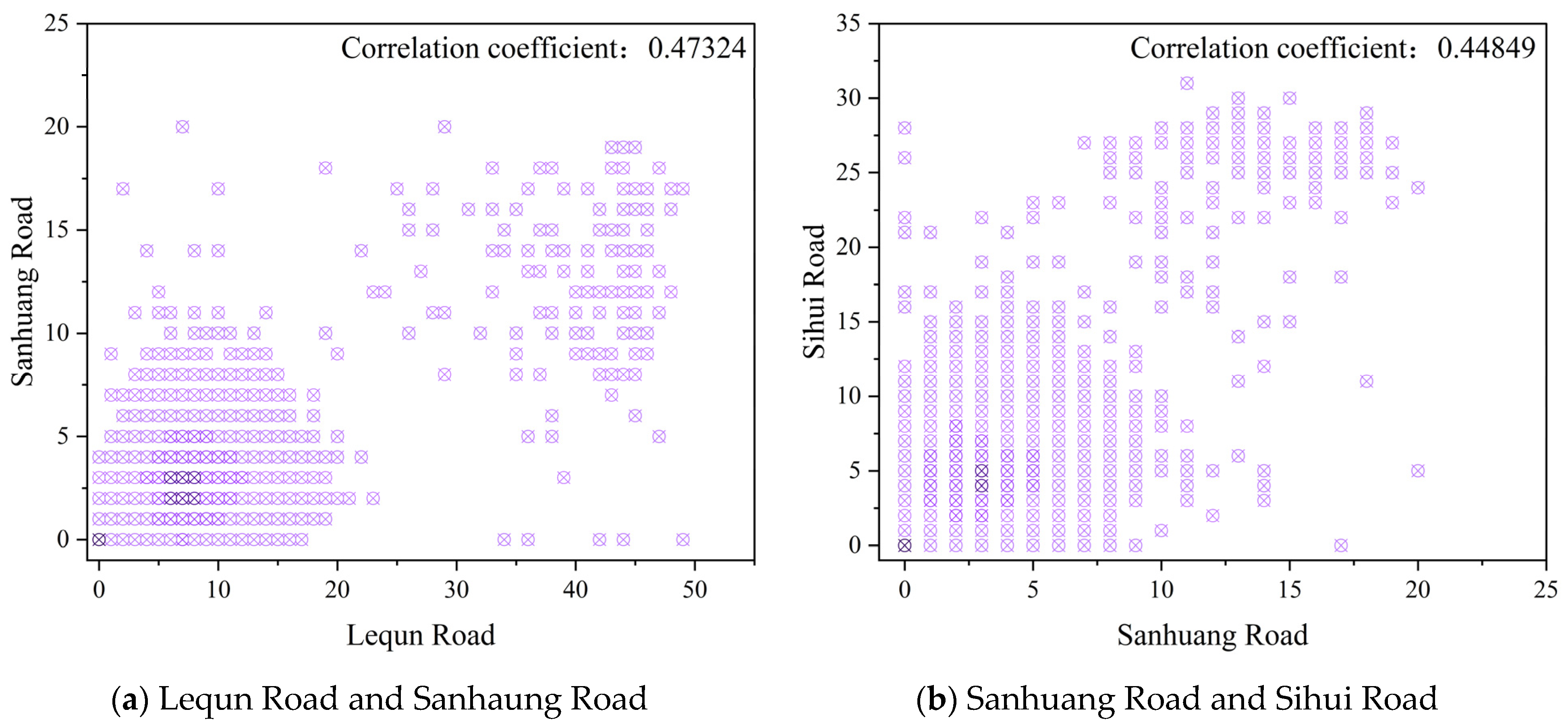
- Physical Location
- (2)
- Semantic Function
Model Design
3.2.3. Fusion
4. Experiments
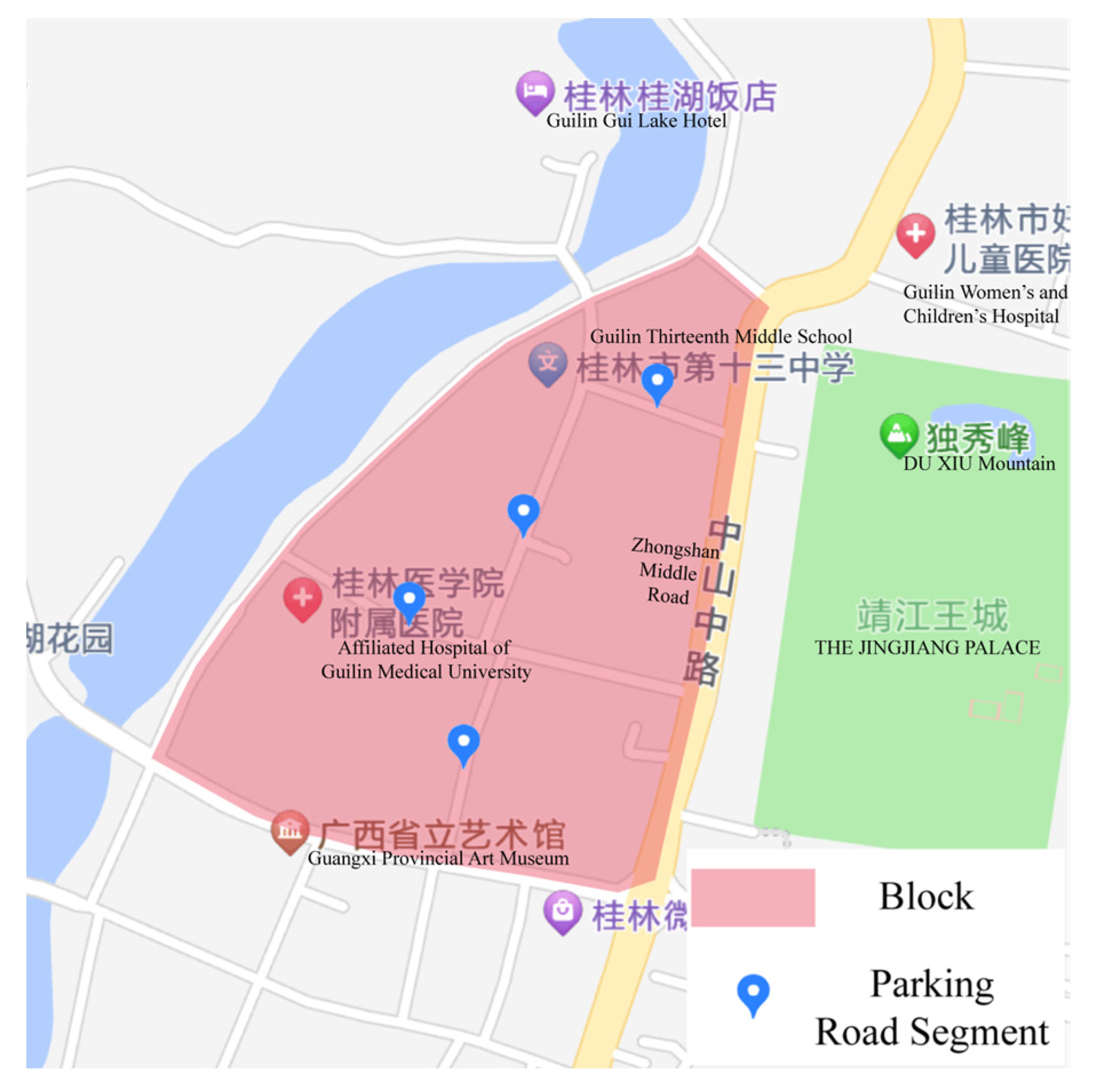
4.1. Datasets
- (1)
- Hour-by-hour weather data from 30 November 2020 to 30 April 2021 for Guilin. Precipitation, wind speed, visibility, and temperature data are screened from it. Data are obtained from the NCEI National Environmental Data website.
- (2)
- The specific scheduling of actual weekdays and holidays is obtained from the holiday scheduling notice issued by the General Office of the State Council of the People’s Republic of China.
- (3)
- Driving path planning and driving distances between different road sections in the region, with data from the Gaode Open Platform.
- (4)
- POI data of different categories within the specific area around each road section, with 23 categories in total, with data from the Gaode Open Platform.
- (5)
- The walking path planning and walking distance between each road section and each POI in the specific area around it, with data from Gaode Open Platform.
4.2. Experimental Settings
4.2.1. Evaluation Metrics
4.2.2. Baselines and Details
- (1)
- Only the P1 component of the overall prediction module in the model is excluded.
- (2)
- Only the P2 component of the overall prediction module in the model is excluded.
- (3)
- The P1 component and the P2 component of the overall prediction module in the model are also excluded.
- (4)
- Only physical adjacency features of the internal distribution prediction module are excluded.
- (5)
- Only the semantic functional similarity relationship features of the internal distribution prediction module are excluded.
4.3. Experimental Results
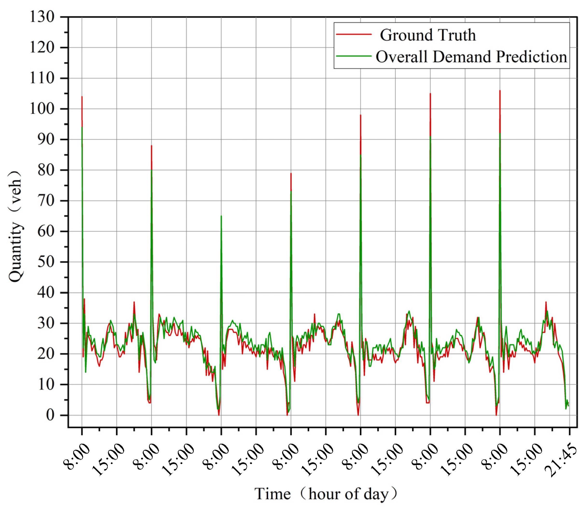
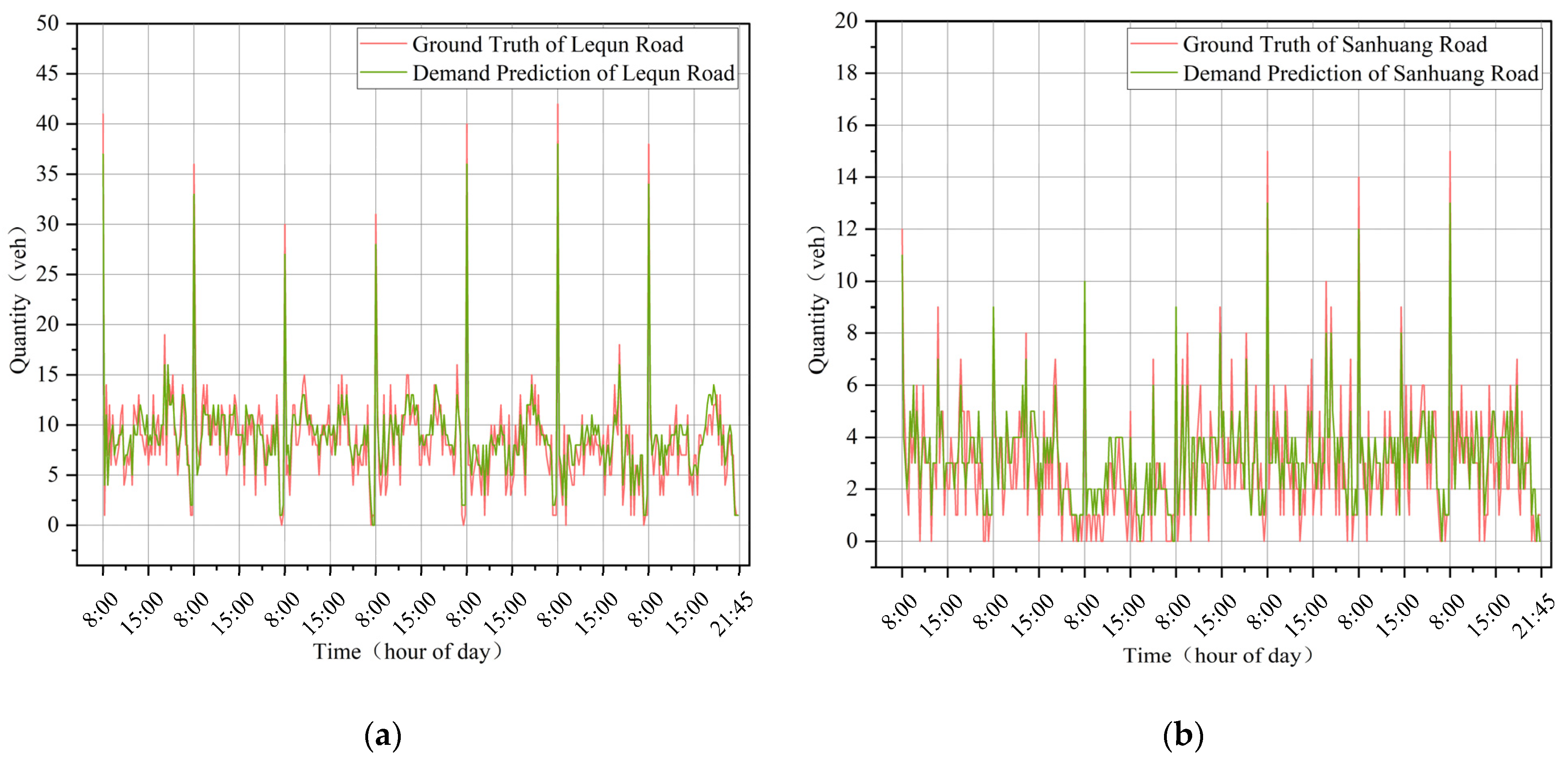
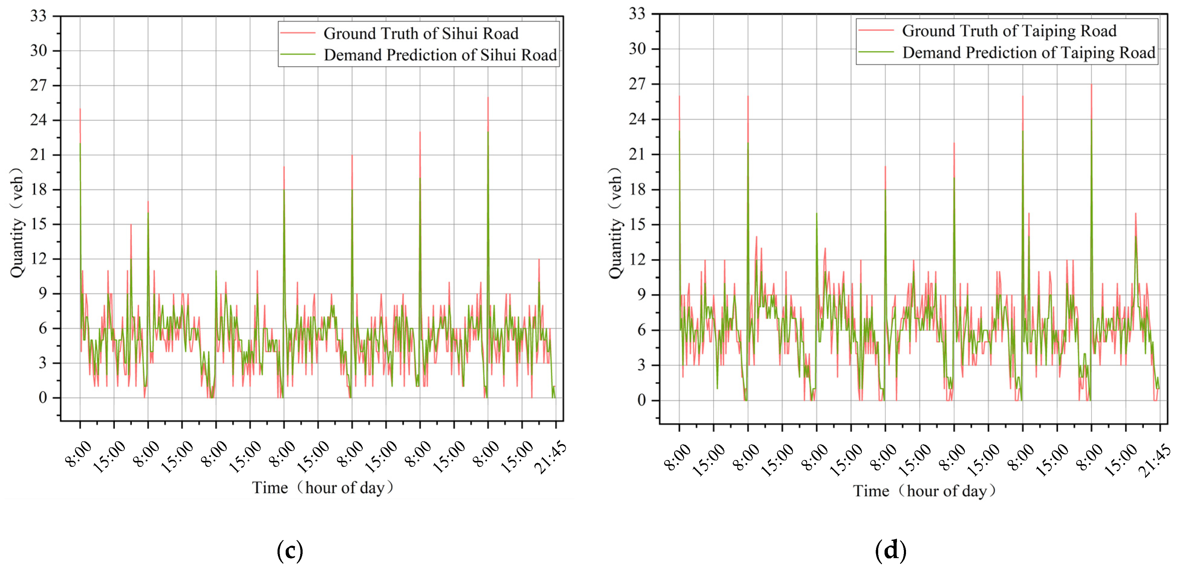
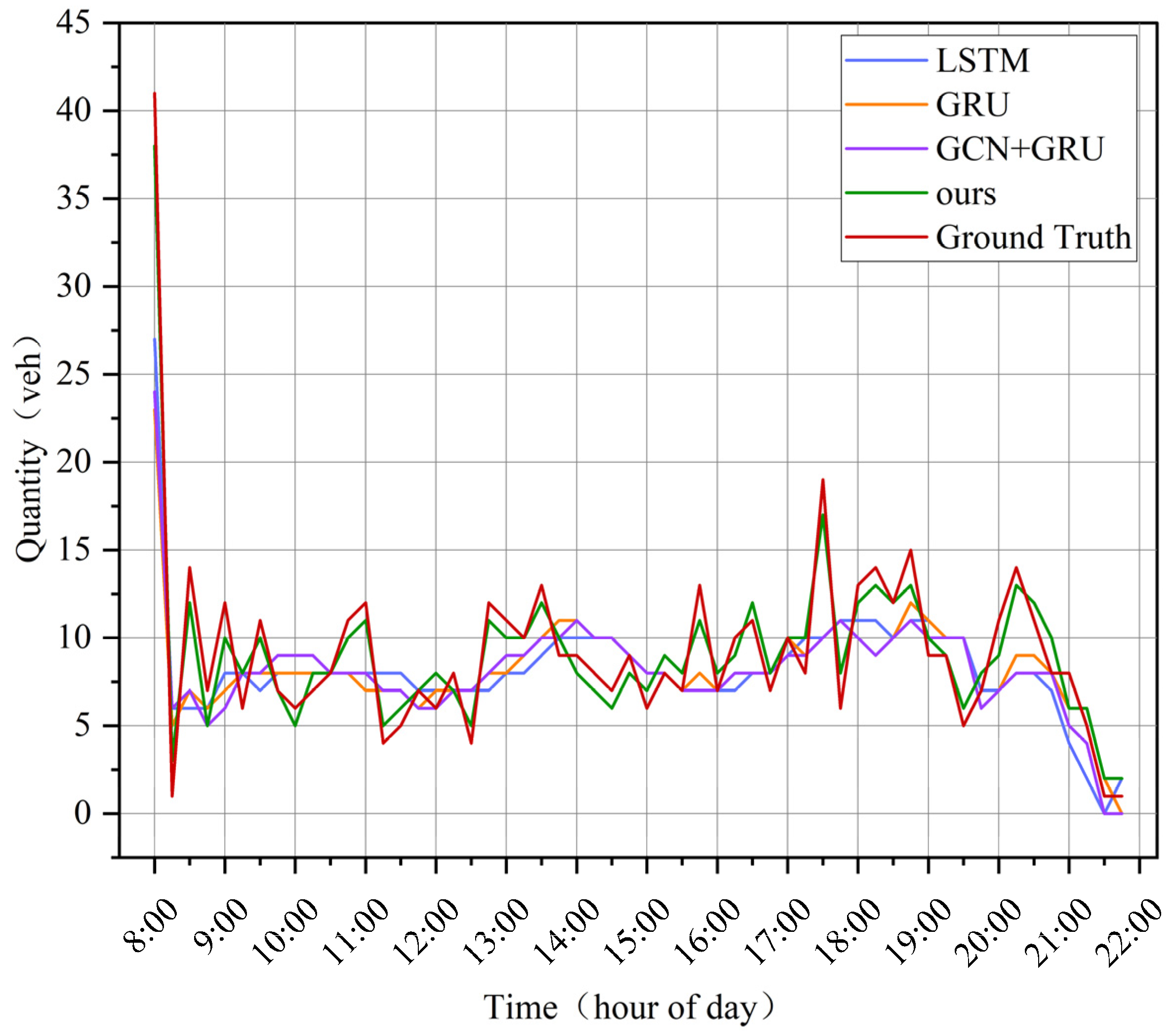
4.3.1. Results Compared with Baselines
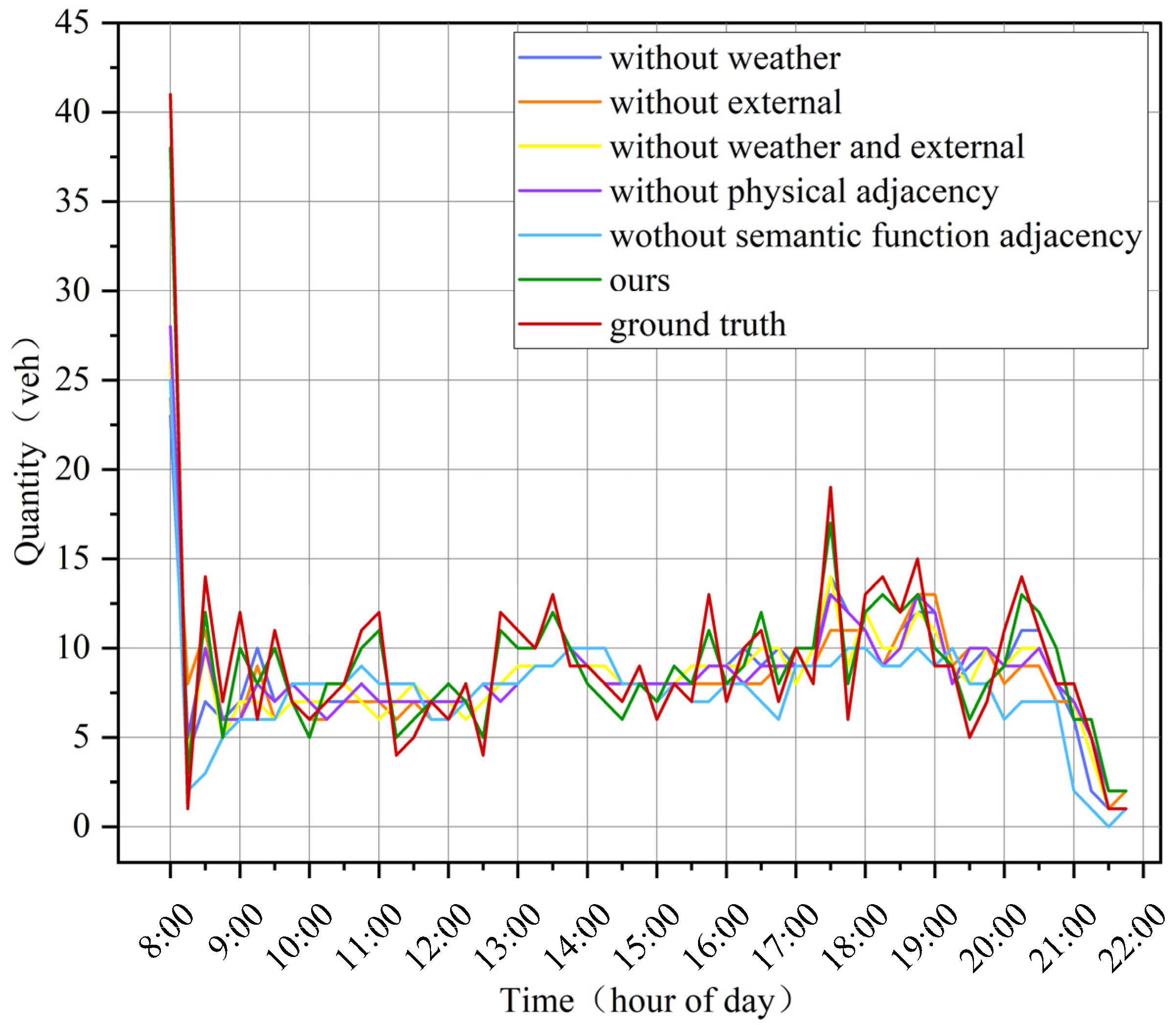
4.3.2. Ablation Experiments with Different Components
5. Conclusions
Author Contributions
Funding
Institutional Review Board Statement
Informed Consent Statement
Data Availability Statement
Conflicts of Interest
References
- Xinhua News Agency. 415 Million Vehicles, More Than 500 Million People! China Releases Latest Motor Vehicle and Driver Data. Available online: http://www.gov.cn/xinwen/2022-12/08/content_5730661.htm (accessed on 6 April 2023).
- Xiao, X.; Jin, Z.; Hui, Y.; Xu, Y.; Shao, W. Hybrid Spatial–Temporal Graph Convolutional Networks for On-Street Parking Availability Prediction. Remote Sens. 2021, 13, 3338. [Google Scholar] [CrossRef]
- Tilahun, S.L.; Di Marzo Serugendo, G.; Angel, I.; Ibeas, A. Cooperative Multiagent System for Parking Availability Prediction Based on Time Varying Dynamic Markov Chains. J. Adv. Transp. 2017, 2017, 1760842. [Google Scholar] [CrossRef]
- Bock, F.; Di Martino, S.; Origlia, A. Smart Parking: Using a Crowd of Taxis to Sense On-Street Parking Space Availability. IEEE Trans. Intell. Transp. Syst. 2020, 21, 496–508. [Google Scholar] [CrossRef]
- On-Street Parking Fee Collection Goes Digital in Central Beijing. Available online: https://global.chinadaily.com.cn/a/201907/02/WS5d1af0b9a3105895c2e7b2bc.html (accessed on 2 July 2019).
- Promote the Construction of Smart Cities to Break the Parking Difficulties in Large Cities. Available online: https://tech.chinadaily.com.cn/a/202103/11/WS604970c5a3101e7ce97436af.html (accessed on 11 March 2021).
- Yang, S.; Ma, W.; Pi, X.; Qian, S. A deep learning approach to real-time parking occupancy prediction in transportation networks incorporating multiple spatio-temporal data sources. Transp. Res. Part C Emerg. Technol. 2019, 107, 248–265. [Google Scholar] [CrossRef]
- Balmer, M.; Weibel, R.; Huang, H. Value of incorporating geospatial information into the prediction of on-street parking occupancy—A case study. Geo-Spat. Inf. Sci. 2021, 24, 438–457. [Google Scholar] [CrossRef]
- Zhao, Z.; Zhang, Y.; Zhang, Y. A Comparative Study of Parking Occupancy Prediction Methods considering Parking Type and Parking Scale. J. Adv. Transp. 2020, 2020, 5624586. [Google Scholar] [CrossRef]
- Hyeonsup, L.; Grant, T.W.; Dua, A.; Joseph, A.; Ziwen, L.; Davis, W.P.; Christopher, R.C. Alternative Approach for Forecasting Parking Volumes. Transp. Res. Procedia 2017, 25, 4171–4184. [Google Scholar]
- Ho, P.W.; Ghadiri, S.M.; Rajagopal, P.; Zainorizuan, M.J.; Yee Yong, L.; Alvin John Meng Siang, L.; Mohamad Hanifi, O.; Siti Nazahiyah, R.; Mohd Shalahuddin, A. Future Parking Demand at Rail Stations in Klang Valley. MATEC Web Conf. 2017, 103, 9001. [Google Scholar] [CrossRef]
- Junbin, X.; Zhiyong, Z.; Jian, R. The Forecasting Model of Bicycle Parking Demand on Campus Teaching and Office District. Procedia-Soc. Behav. Sci. 2012, 43, 550–557. [Google Scholar]
- Swanson, H.A. The Influence of Central Business District Employment and Parking Supply on Parking Rates. ITE J. 2004, 74, 28–30. [Google Scholar]
- Amini, M.H.; Karabasoglu, O.; Ilić, M.D.; Boroojeni, K.G.; Iyengar, S.S. ARIMA-based demand forecasting method considering probabilistic model of electric vehicles’ parking lots. In Proceedings of the 2015 IEEE Power & Energy Society General Meeting, Denver, CO, USA, 26–30 July 2015; pp. 1–5. [Google Scholar]
- Rajabioun, T.; Ioannou, P.A. On-Street and Off-Street Parking Availability Prediction Using Multivariate Spatiotemporal Models. IEEE Trans. Intell. Transp. Syst. 2015, 16, 2913–2924. [Google Scholar] [CrossRef]
- Ye, X.; Wang, J.; Wang, T.; Yan, X.; Ye, Q.; Chen, J. Short-Term Prediction of Available Parking Space Based on Machine Learning Approaches. IEEE Access 2020, 8, 174530–174541. [Google Scholar] [CrossRef]
- Fan, J.; Hu, Q.; Tang, Z. Predicting vacant parking space availability: An SVR method with fruit fly optimisation. IET Intell. Transp. Syst. 2018, 12, 1414–1420. [Google Scholar] [CrossRef]
- Li, T.; Wu, X.; Zhang, J. Time Series Clustering Model based on DTW for Classifying Car Parks. Algorithms 2020, 13, 57. [Google Scholar] [CrossRef]
- Tamrazian, A.; Qian, Z.S.; Rajagopal, R. Where is My Parking Spot?: Online and Offline Prediction of Time-Varying Parking Occupancy. Transp. Res. Rec. 2015, 2489, 77–85. [Google Scholar] [CrossRef]
- Peng, L.; Li, H. Searching parking spaces in urban environments based on non-stationary Poisson process analysis. In Proceedings of the 2016 IEEE 19th International Conference on Intelligent Transportation Systems (ITSC), Rio de Janeiro, Brazil, 1–4 November 2016; pp. 1951–1956. [Google Scholar]
- Zheng, L.; Xiao, X.; Sun, B.; Mei, D.; Peng, B. Short-Term Parking Demand Prediction Method Based on Variable Prediction Interval. IEEE Access 2020, 8, 58594–58602. [Google Scholar] [CrossRef]
- Xiao, J.; Lou, Y.; Frisby, J. How likely am I to find parking?—A practical model-based framework for predicting parking availability. Transp. Res. Part B Methodol. 2018, 112, 19–39. [Google Scholar] [CrossRef]
- Li, M.; Li, M.; Liu, B.; Liu, J.; Liu, Z.; Luo, D. Spatio-Temporal Traffic Flow Prediction Based on Coordinated Attention. Sustainability 2022, 14, 7394. [Google Scholar] [CrossRef]
- Wang, J.; Gao, J.; Wei, D. Electric load prediction based on a novel combined interval forecasting system. Appl. Energ. 2022, 322, 119420. [Google Scholar] [CrossRef]
- Tao, Q.; Liu, F.; Li, Y.; Sidorov, D. Air Pollution Forecasting Using a Deep Learning Model Based on 1D Convnets and Bidirectional GRU. IEEE Access 2019, 7, 76690–76698. [Google Scholar] [CrossRef]
- Chung, J.; Gulcehre, C.; Cho, K.; Bengio, Y. Empirical Evaluation of Gated Recurrent Neural Networks on Sequence Modeling. arXiv 2014. [Google Scholar] [CrossRef]
- Cho, K.; van Merrienboer, B.; Gulcehre, C.; Bahdanau, D.; Bougares, F.; Schwenk, H.; Bengio, Y. Learning Phrase Representations using RNN Encoder-Decoder for Statistical Machine Translation. arXiv 2014. [Google Scholar] [CrossRef]
- Zhu, L.; Laptev, N. Deep and Confident Prediction for Time Series at Uber. In Proceedings of the 2017 IEEE International Conference on Data Mining Workshops (ICDMW), New Orleans, LA, USA, 18–21 November 2017; IEEE: Ithaca, NY, USA, 2017; pp. 103–110. [Google Scholar]
- Xue, J.; Shen, B. A novel swarm intelligence optimization approach: Sparrow search algorithm. Syst. Sci. Control Eng. 2020, 8, 22–34. [Google Scholar] [CrossRef]
- Bahdanau, D.; Cho, K.; Bengio, Y. Neural Machine Translation by Jointly Learning to Align and Translate. arXiv 2014. [Google Scholar] [CrossRef]
- An, G.; Jiang, Z.; Chen, L.; Cao, X.; Li, Z.; Zhao, Y.; Sun, H. Ultra Short-Term Wind Power Forecasting Based on Sparrow Search Algorithm Optimization Deep Extreme Learning Machine. Sustainability 2021, 13, 10453. [Google Scholar] [CrossRef]
- Nie, Y.; Yang, W.; Chen, Z.; Lu, N.; Huang, L.; Huang, H. Public Curb Parking Demand Estimation with POI Distribution. IEEE Trans. Intell. Transp. Syst. 2022, 23, 4614–4624. [Google Scholar] [CrossRef]
- Xia, B.; Ruan, Y. Function Replacement Decision-Making for Parking Space Renewal Based on Association Rules Mining. Land 2022, 11, 156. [Google Scholar] [CrossRef]
- Rong, Y.; Xu, Z.; Yan, R.; Ma, X. Du-Parking: Spatio-Temporal Big Data Tells You Realtime Parking Availability. In Proceedings of the 24th ACM SIGKDD International Conference on Knowledge Discovery & Data Mining, London, UK, 19–23 August 2018; ACM: New York, NY, USA, 2018; pp. 646–654. [Google Scholar]
- Fan, J.; Hu, Q.; Xu, Y.; Tang, Z. Predicting Vacant Parking Space Availability: A Long Short-Term Memory Approach. IEEE Intell. Transp. Syst. Mag. 2022, 14, 129–143. [Google Scholar] [CrossRef]
- Kipf, T.N.; Welling, M. Semi-Supervised Classification with Graph Convolutional Networks. arXiv 2016. [Google Scholar] [CrossRef]
- Zhao, D.; Ju, C.; Zhu, G.; Ning, J.; Luo, D.; Zhang, D.; Ma, H. MePark: Using Meters as Sensors for Citywide On-Street Parking Availability Prediction. IEEE Trans. Intell. Transp. Syst. 2022, 23, 7244–7257. [Google Scholar] [CrossRef]
- Kotb, A.O.; Shen, Y.; Zhu, X.; Huang, Y. iParker-A New Smart Car-Parking System Based on Dynamic Resource Allocation and Pricing. IEEE Trans. Intell. Transp. Syst. 2016, 17, 2637–2647. [Google Scholar] [CrossRef]
- Liu, K.S.; Gao, J.; Wu, X.; Lin, S. On-Street Parking Guidance with Real-Time Sensing Data for Smart Cities. In Proceedings of the 2018 15th Annual IEEE International Conference on Sensing, Communication, and Networking (SECON), Hong Kong, China, 11–13 June 2018; pp. 1–9. [Google Scholar]
- Wang, J.; Wang, Z.; Li, J.; Wu, J. Multilevel Wavelet Decomposition Network for Interpretable Time Series Analysis. arXiv 2018. [Google Scholar] [CrossRef]


| Lequn Road | Sanhuang Road | Sihui Road | Taiping Road | |
|---|---|---|---|---|
| Lequn Road | 1 | 0.84416343 | 0.89911893 | 0.95502897 |
| Sanhuang Road | 0.84416343 | 1 | 0.84044845 | 0.76167333 |
| Sihui Road | 0.89911893 | 0.84044845 | 1 | 0.78182478 |
| Taiping Road | 0.95502897 | 0.76167333 | 0.78182478 | 1 |
| Road | The Number of Parking Spaces |
|---|---|
| Lequn Road | 42 |
| Sanhuang Road | 18 |
| Sihui Road | 26 |
| Taiping Road | 29 |
| Model | RMSE | MAE |
|---|---|---|
| HA | 4.089 | 2.858 |
| ARIMA | 3.885 | 2.653 |
| LSTM | 3.354 | 2.568 |
| GRU | 3.347 | 2.556 |
| GCN+GRU | 3.248 | 2.505 |
| HA+B&D | 3.857 | 2.795 |
| ARIMA+B&D | 3.581 | 2.450 |
| LSTM+B&D | 2.494 | 1.917 |
| GRU+B&D | 2.501 | 1.915 |
| GCN+GRU+B&D | 2.437 | 1.882 |
| ours | 2.254 | 1.791 |
| Model | RMSE | MAE |
|---|---|---|
| without weather | 2.385 | 1.868 |
| without external | 2.380 | 1.872 |
| without weather and external | 2.429 | 1.874 |
| without physical adjacency | 2.418 | 1.898 |
| without semantic function adjacency | 2.441 | 1.913 |
| ours | 2.254 | 1.791 |
Disclaimer/Publisher’s Note: The statements, opinions and data contained in all publications are solely those of the individual author(s) and contributor(s) and not of MDPI and/or the editor(s). MDPI and/or the editor(s) disclaim responsibility for any injury to people or property resulting from any ideas, methods, instructions or products referred to in the content. |
© 2023 by the authors. Licensee MDPI, Basel, Switzerland. This article is an open access article distributed under the terms and conditions of the Creative Commons Attribution (CC BY) license (https://creativecommons.org/licenses/by/4.0/).
Share and Cite
Wang, T.; Li, S.; Li, W.; Yuan, Q.; Chen, J.; Tang, X. A Short-Term Parking Demand Prediction Framework Integrating Overall and Internal Information. Sustainability 2023, 15, 7096. https://doi.org/10.3390/su15097096
Wang T, Li S, Li W, Yuan Q, Chen J, Tang X. A Short-Term Parking Demand Prediction Framework Integrating Overall and Internal Information. Sustainability. 2023; 15(9):7096. https://doi.org/10.3390/su15097096
Chicago/Turabian StyleWang, Tao, Sixuan Li, Wenyong Li, Quan Yuan, Jun Chen, and Xiang Tang. 2023. "A Short-Term Parking Demand Prediction Framework Integrating Overall and Internal Information" Sustainability 15, no. 9: 7096. https://doi.org/10.3390/su15097096
APA StyleWang, T., Li, S., Li, W., Yuan, Q., Chen, J., & Tang, X. (2023). A Short-Term Parking Demand Prediction Framework Integrating Overall and Internal Information. Sustainability, 15(9), 7096. https://doi.org/10.3390/su15097096