Article

A Short-Term Parking Demand Prediction Framework Integrating Overall and Internal Information

1
Guangxi Key Laboratory of Intelligent Transportation System, School of Architecture and Transportation Engineering, Guilin University of Electronic Technology, Guilin 541004, China
2
School of Architecture and Transportation Engineering, Guilin University of Electronic Technology, Guilin 541004, China
3
State Key Laboratory of Automotive Safety and Energy, School of Vehicle & Mobility, Tsinghua University, Beijing 100084, China
4
School of Transportation, Southeast University, Nanjing 210096, China
5
Guangxi Communications Design Group Co., Ltd., Nanning 530022, China
*
Authors to whom correspondence should be addressed.
Sustainability 2023, 15(9), 7096; https://doi.org/10.3390/su15097096
Submission received: 23 March 2023 / Revised: 16 April 2023 / Accepted: 18 April 2023 / Published: 24 April 2023

Abstract

:
With the development of smart cities and smart transportation, cities can gradually provide people with more information to facilitate their life and travel, and parking is also inseparable from both of them. Accurate on-street parking demand prediction can improve parking resource utilization and parking management efficiency, as well as potentially improve urban traffic conditions. Previous parking demand prediction methods seldom consider the correlation between the parking demand of a road section and its surroundings. Therefore, in order to capture the correlation of parking demand in the temporal and spatial dimensions as carefully as possible and enrich the relevant features in the prediction model so as to achieve more accurate prediction results, we designed a parking demand prediction structure that considers different features from two perspectives: overall and internal. We used gated recurrent units (GRU) to extract demand influences in the temporal dimension. The GRU is used in combination with a graph convolutional neural network (GCN) to extract demand influencing factors in the spatial dimension. Additionally, a more detailed representation is designed to express spatial dimensional features. Then, based on the historical parking demand features extracted using encoder–decoder, we fuse the extracted spatio-temporal features with them to finally obtain an on-street parking demand prediction model combining the overall and the internal information. By combining them, we can integrate more correlation factors to achieve a more accurate parking demand prediction. The performance of the model is evaluated by real parking data in Xiufeng District of Guilin. The results show that the proposed model achieves good prediction performance compared with other baselines. In addition, we also design feature ablation experiments. Through the comparison of the results, we find that each feature considered in the proposed model is important in parking demand prediction.

1. Introduction

With the continuous development of cities, social progress, and population increase, traveling by car has become a normal part of people’s life, and cars have entered thousands of households, becoming consumer goods and necessities for ordinary families. However, the increasing number of motor vehicles does not match the capacity of urban parking facilities. According to the latest data released by the Ministry of Public Security of China on 8 December 2022, by the end of November 2022, the number of motor vehicles in the country reached 415 million, of which the number of cars reached 318 million. The number of motor vehicle drivers exceeded 500 million, of which the number of car drivers reached 463 million. At present, the total number of motor vehicles and drivers are the highest in the world. In recent years, the average annual increment of car ownership exceeds 20 million, the number of cars per 1000 people has reached 225, and the average number of cars per 100 households has reached 60 [1]. Most of the public parking lots in cities are business paid parking lots, or traffic or commercial parking lots attached to shopping malls, hospitals, transportation hubs, etc. Therefore, on-street parking is usually the choice of people [2]. When the number of on-street parking spaces cannot keep up with the large demand caused by the rapid increase of motor vehicles, it will easily cause traffic congestion [3], road safety and other problems, and there will be social problems in terms of environment and energy [4]. The prediction results of on-street parking demand can provide drivers with helpful information, thus improving the utilization of urban parking facilities. It is also one of the foundations of urban traffic control and guidance, and is one of the main functions of intelligent transportation systems (ITS) [2].
In current studies, predictions of parking demand generally require the use of large amounts of historical data. Generally, on-street parking information needs to be captured by various facilities. In the past, parking information was not available accurately due to technical, equipment, and economic constraints. Now, with advances in technology, some cities have been or are being equipped with advanced equipment to obtain accurate parking information. These facilities provide access to a large and accurate amount of historical on-street parking data, such as underground geomagnetic sensors, high-level video surveillance [5,6], etc. However, while such a facility can collect very accurate and valuable parking data, it also entails high installation and maintenance costs. For the time being, many places in China do not have all these facilities installed due to restrictions related to urban construction. Some areas are currently using handheld entry devices for parking information entry. Although the cost of such equipment is low, it requires the employment of certain human resources, and in many cases there will be errors in the vehicle parking and driving out time.
In the construction of smart cities, the managers expect that the parking lot is not only in a simple location that provides parking and that they can charge for it, but also that it will assist the city in the coordination of traffic aspects. Therefore, it will be helpful if the parking demand information can be used to analyze the changes of urban parking demand at the temporal and spatial levels, to grasp its global state, or even to combine multiple sources of data around parking resources, such as considering the surrounding traffic network [7], urban points of interest [8], weather, holidays, etc., or considering the relevant attributes of parking lots [9]. A more scientific parking allocation or inducement strategy can help the management of parking resources in the city, or even can provide reference to the construction planning of parking facilities resources from a higher level, at least from the regional level. Therefore, not only short-term parking demand prediction has been receiving attention, but also grasping the changes of parking demand from a higher level for effective management is the goal of much research.
Previous studies on parking demand forecasting can be broadly divided into two types. One type of prediction is conducted from a static traffic perspective. This type of approach usually uses some general characteristics to make macro-level forecasts. The other one is to forecast from historical data, using some statistical or machine learning methods. We will introduce the progress of related research in detail in Section 2.
In this paper, we propose a parking demand prediction structure that combines the overall demand and internal distribution. It is able to combine multiple characteristics of road segments in the temporal dimension and correlations with other road segments in the spatial dimension.
Specifically, we construct a demand prediction structure that combines a region as a whole with an internal distribution. In the demand prediction for the region as a whole, we first use an encoder–decoder to extract features from the historical parking demand. After that, we use a gated recurrent unit (GRU) to capture the relevant features of the overall block and incorporate them into the demand features to achieve the forecast of the region as a whole. For the prediction of internal distribution, two graph structures, physical location relationship, and semantic functional similarity of road segments are constructed, and these two correlation features are extracted using two graph convolutional neural networks (GCN), respectively. Then, they are combined with the distribution features also extracted using the encoder–decoder to achieve the prediction of internal demand distribution. Finally, the prediction results of the overall block are combined with the prediction results of the internal distribution to obtain the prediction results of the parking demand for each section in the block. We use real parking business order data in Guilin to evaluate the model. The results show that our proposed model has good performance.
In summary, the main contributions of this paper are as follows:
  • A multi-parking prediction model combining the whole and local aspects is constructed by combining two aspects: the whole block and its interior. Compared with the traditional multi-parking prediction task, the approach splits and transforms the pure point prediction task and is able to capture more factors associated with it. Thus, the accuracy of parking demand prediction improves by using the more factors.
  • For the prediction model, a combination of GCN and GRU is chosen to effectively extract temporal and spatial information from the data. The model is based on historical parking demand data, and while using encoder–decoder to extract the characteristics of demand itself. It also fuses the temporal and spatial factors that have an impact on the parking demand of road sections. The combination of such multiple neural network layers obtains the required information in a complex urban road network. Thus, it fuses multiple sources of data effectively and obtains more desirable prediction results.
  • A variety of features and influencing factors related to parking demand are analyzed. In addition to considering some inherent external factors, such as weather and holidays, improved spatial class features are also added. The features use more detailed representation methods, such as representing the spatial distance relationship between road sections using their driving times, and representing their semantic functions using the number and distance of various types of points of interest around the road sections, etc. At the same time, these analyzed features are also divided and incorporated into the model from both overall and local perspectives to enrich the influencing factors from the input perspective as meticulously as possible.
  • The validation is performed using a real parking dataset from Xiufeng District of Guilin. The good performance of the model in this paper is reflected from the validation results, especially this structure of combining the whole block with the block interior. In addition, the robustness of the model is also reflected by using such a dataset with general accuracy. Finally, the design of the ablation experiment and the comparison of the results demonstrate the importance of considering each feature in the model.

2. Related Work

In the related field of parking, there are many scholars who have made considerable contributions to the development of the field. In this section, we mainly summarize the work related to parking demand prediction in terms of relevant forecasting methods.

2.1. Parking Demand Prediction Based on Static Traffic

Earlier, instead of using a large amount of micro-level historical parking data as the main basis for prediction, many studies on parking demand prediction have widely used static traffic demand prediction models. These mainly include prediction models based on land use, traveling, and socio-economic activity characteristics that mostly focus on some inherent characteristic values, such as parking generation rate models based on the relationship between land use properties and parking demand generation rates, trip attraction models that consider the amount of regional motor vehicle trips attracted, and parking demand–supply prediction models based on parking service levels, etc. [10,11,12,13]. For example, Hyeonsup et al. proposed an allocation model using a generalized cost approach through a sensitivity analysis of parking generation rate, walking speed, and space finding time, which enabled a more detailed prediction of the number of parking spaces [10]. Swanson et al. analyzed and explained the interrelationships obtained among employment, parking demand, and parking generation rate by studying the factors affecting the parking generation rate in the central business district, and obtained a prediction model for parking generation rate eventually [13]. Ho et al. studied the factors influencing parking demand in terms of population, car parking, new car registrations, and rail passenger capacity, and predicted future parking demand using linear regression [11]. However, the models used in such work are mostly unsophisticated and also rely more on traditional theoretical analysis and models for parking prediction, all of which may suffer from problems such as long-range applicability and credibility.

2.2. Parking Demand Prediction Based on Machine Learning

The more common prediction models nowadays are based on a large amount of historical parking data and use more advanced methods such as machine learning neural network [2,7,14,15,16]. Various models have been proposed for accurate parking availability prediction. For example, Amini et al. proposed an electricity demand forecasting method considering the charging demand of electric vehicle parking lots using historical load data, which is based on an autoregressive integrated moving average (ARIMA) model for medium-term demand forecasting and has been shown to have high forecasting accuracy through its simulation results [14]. In addition, the more difficult and also more accurate method is also widely used. Xiao et al. proposed a parking availability forecasting model based on the spatio-temporal convolutional blocks constructed with graph convolutional networks, gated linear units, and one-dimensional convolutional neural networks to obtain instantaneous spatio-temporal correlation [2]. A wide range of techniques have been used to model parking prediction, in addition to the above-mentioned neural networks such as autoregressive integrated moving average, gated unit, and convolution, support vector regression (SVR) [17], multivariate autoregression [15], and clustering [18,19] are also used to predict parking demand. Another way of parking availability prediction is to analyze and predict parking demand based on the parking process [20,21,22]. For example, Zheng et al. constructed a parking demand prediction model using Markovian generation and extinction process, and gave a method to determine the forecasting interval based on the trend of the number of parking spaces according to the different parameters of the drivers’ arrival and departure [21]. However, such kind of methods rely on a lot of assumptions and are less adaptable in the real environment. Demand forecasting using machine learning methods have achieved better performance, but they mainly analyze the characteristics of the historical data itself and do not take enough account of other influencing factors, so deep learning because of higher accuracy is also widely used in the analysis and prediction of parking demand.
In recent years, with the rapid development of artificial intelligence, deep learning has been widely used in various types of prediction, including traffic flow [23], passenger demand, electricity load [24], air pollution [25], etc., with its high adaptability and excellent performance. Its excellent performance in fields such as image recognition and natural language processing also proves the effectiveness of neural networks in dealing with multivariate, nonlinear, and nonstationary data, and implies the effectiveness in dealing with time series prediction problems as well. The proposition of neural network methods such as LSTM and GRU [26,27] not only enhance the model’s ability to capture features in long sequences, but also effectively improve the accuracy of prediction results while avoiding the gradient explosion problem that tends to occur in RNNs. The U.S. technology company Uber has also designed a model with multiple LSTMs to predict the ride information of passengers in each city [28]. In addition, more and more optimization algorithms are being used to further improve the performance of these models [16,29,30,31], and more factors are being considered into the models, such as city points of interest (POIs) [32]. Xia et al. built a decision support model for parking space function substitution to share the burden of parking as much as possible through association patterns with other city points of interest (POIs) [33]. However, both the real-time parking availability prediction method named Du-Parking [34] proposed by Rong et al. and the multi-step LSTM prediction model [35] proposed by Fan et al., though their results proved to be superior to several classical benchmark models, including gated recursive units (GRU), stacked autoencoders (SAE), SVR models, and back propagation neural networks (BPNN), the inputs to the models are limited to 2D or 3D grid data in Euclidean space.
The proposition of GCN effectively extends convolution to non-Euclidean graph data [36] and is currently being widely used in various predictions presently. Yang et al. made multiple heterogeneous structured traffic data sources as input to extract the spatial relationships of traffic flows in a large-scale network using graph convolutional neural networks while incorporating LSTM to predict parking occupancy in a neighborhood in real time with excellent results [7]. Zhao et al. proposed a sensor for predicting real-time citywide on-street parking availability deployment at a fine-grained temporal level based on simple parking fee transaction data and other contextual data, while designing an iterative prediction mechanism that combines inflow prediction and parking duration prediction with a multi-graph convolutional neural network (MGCN) and LSTM to capture complex spatio-temporal correlations [37]. In this paper, graph convolution is similarly used to capture correlations from a variety of different graph structures, including physical adjacencies and semantically similar features.
Although parking demand prediction can alleviate many parking problems, however, considering it from another perspective, it may also cause other problems. For example, the prediction results of demand help drivers to make the selection of target parking sections in advance, but it may also cause the problem of multiple cars competing for parking spaces. Currently, there are a number of solutions to the parking resource allocation problem, such as parking space reservation [38]. However, on-street parking spaces are not available as a resource that can be reserved and made in advance, and such an approach is more suitable for off-street parking. An online real-time parking guidance system is more suitable, for example, on-street parking recommendations can be made in real time based on the prediction of available parking spaces [39], and although there is no research on parking guidance in this paper, reasonable guidance can effectively assist parking management and give greater play to the role of parking demand prediction to solve some problems in parking in practical scenarios.

3. Materials and Methods

In this section, we pose the problem about predicting on-street parking demand. Accordingly, we analyze the characteristics related to parking demand prediction in terms of both overall demand and internal distribution factors of the block, and then, we construct the prediction model.

3.1. Preliminary

Given a parking area where the arrival and departure times of vehicles are known for each road section, multiple sources of data around the area are obtained and relevant features are extracted from them, such as the road network, weather, points of interest (POI), holidays, and so on. By using these known data and relevant features, we aim to predict the future parking demand in short-term time intervals and provide a reliable basis for parking management in the block and internal road sections.
When pre-processing historical parking order data based on the proposed problem described above, the main processing process is as follows:
Dividing the time axis by the same time interval Δ , i.e., 15 min, yields time series labels like { 1 , 2 , , T , T + 1 , } , where [ ( t 1 ) Δ ,   t Δ ] denotes the t -th time interval. The historical parking orders belonging to the interval are integrated according to the time interval, and the parking inflow quantity sequence [ Q 1 V , Q 2 V , , Q t V ] for the whole block V and the parking inflow quantity sequence [ Q 1 i , Q 2 i , , Q t i i V ] for each section within the block are obtained respectively for each time interval, and the demand percentage sequence [ d 1   i , d 2   i , , d t   i i V ] of the parking demand of each section in the whole block is calculated.
The integrated data contains a lot of randomness and uncertainty fundamentally, and it will be constantly perturbed with the role of uncertainty factors around the essential trend of parking demand at fixed time intervals. It will lead to results showing large fluctuations. In order to reduce the adverse effects of the randomness in the parking demand data on the forecasts, Wavelet Transform (WT) is used to reduce the noises of the demand series data before using them [40].
The following are the main steps of wavelet noise reduction. Firstly, the number of layers of wavelet decomposition is determined to decompose the signal. After that, the threshold value of the detail signal under each decomposition layer is determined, which is used to quantize the detail signal. Finally, the detailed signal and the approximation signal after processing by the threshold are reconstructed to get the number of area requirements [ q 1 , q 2 , , q T ] after noise reduction processing.
Based on the above pre-processed data, the parking demand prediction model of this paper is constructed. The main structure is shown in Figure 1, and the main body is divided into two parts: the demand forecast of the whole block and the demand distribution forecast within the block.
(1)
Overall Parking Demand Prediction of Block
In this module, the training of the model is used to achieve the prediction of parking demand for a region. The training part of the overall parking demand prediction model uses the historical total parking demand sequence of the block obtained by extracting aggregates from business orders and the implicit features affecting the overall demand as samples. It uses the demand for the next time interval as the target to achieve the overall parking demand forecast.
(2)
Parking Demand Distribution Prediction within Block
In this module, distribution prediction within the block is also achieved by training the model. The proportional sequence of the owning demand of each road segment within the block is extracted from the total regional demand sequence. The proportional sequence, together with the implicit features of the graph structure containing the correlation between the internal road segments, is used as a sample of the model for training. The distribution of the proportional situation in the next time interval is used as the target to obtain the prediction results of the demand distribution within the block.
Finally, the results of the two modules are integrated to obtain the prediction results of the parking demand of each road section.

3.2. Parking Demand Prediction of Road Sections

3.2.1. Overall Parking Demand Prediction of Block

This section describes how to predict the demand for the ( T + 1 ) -th time interval for regional parking. This section should combine with the internal demand distribution prediction to obtain the final parking demand forecast for each road section.
Characterization of the multi-source data reveals that parking demand forecasts on a regional basis are influenced by a number of external factors. All of the factors are characterized by constant variation over time. Adding these features while using historical parking data can help the model capture its temporal correlation with the input historical demand better.

Feature Analysis

Analyzed from the perspective of the whole block, there are three main time-varying characteristics that affect the parking demand of the whole block, and these characteristics are modeled by different modules according to the differences presented by the characteristics themselves.
(1)
Weather
A weather feature vector f t W is defined, which represents the weather feature vector at the t -th time interval. The vector consists of the following features: precipitation, wind speed, visibility, and temperature. Detailed weather data are obtained from the NCEI National Environmental Data website. Since the minimum unit of weather data we obtain is an hour, which does not match the statistical duration of each demand data, we fit the weather data every 15 min using a linear interpolation method. Linear interpolation is a relatively simple interpolation method. It uses an interpolation function that takes a straight line between two interpolation nodes as an approximate replacement of the original function. Thus, the value of a node in the interpolation interval that may not have been available before can be obtained. We perform linear interpolation of two adjacent hourly weather data to obtain specific data for every 15 min. We performed such interpolation calculations for rainfall, wind speed, visibility, and temperature.
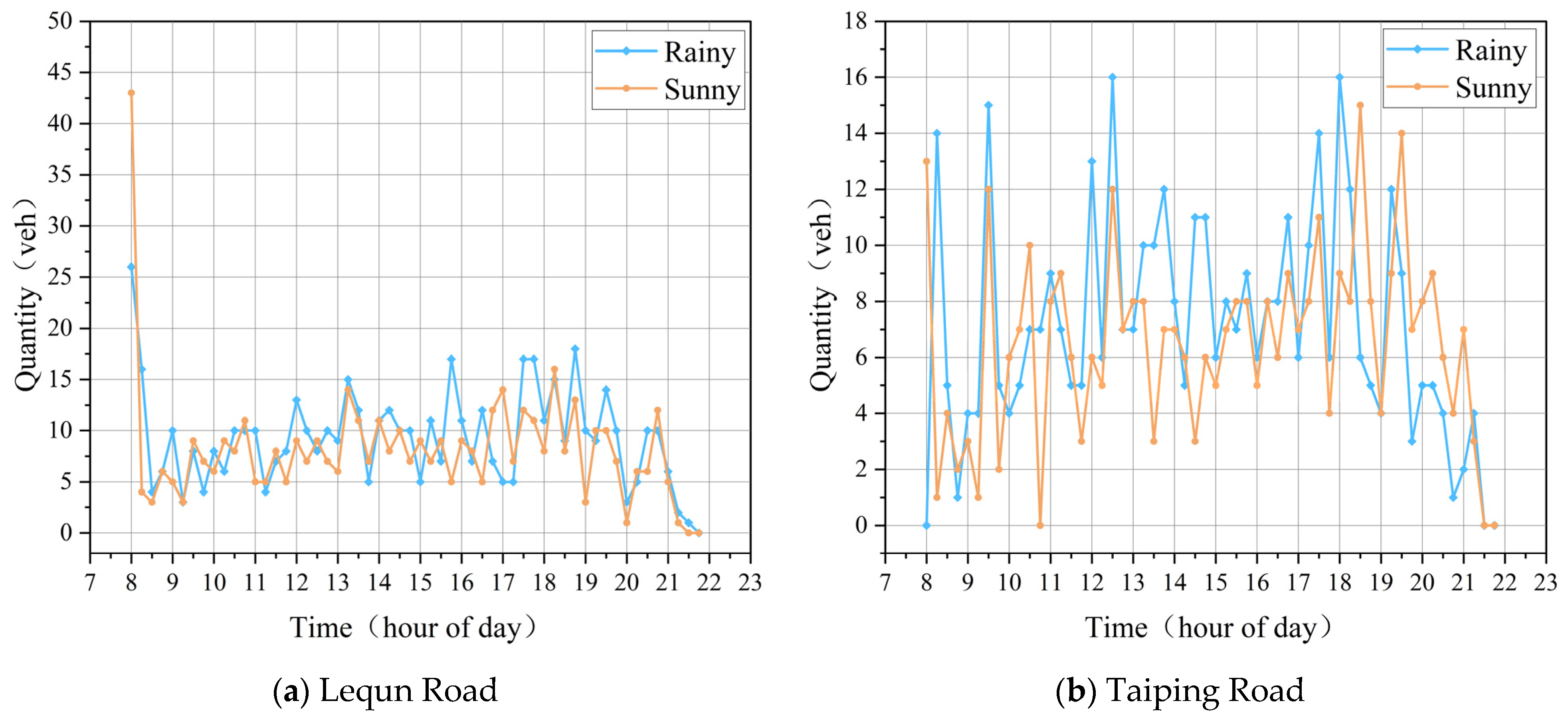
It is found statistically that different weather conditions, such as sunny or rainy, may lead to different demand representations. While severe weather conditions, such as heavy rain, snowfall, low temperatures, and strong winds may also lead to different demand than usual. At the same time, this dynamic effect of weather exists at different times and regions, and for blocks with different attributes, the same weather conditions may also lead to different demand representations. As shown in Figure 2, the demand of Lequn Road, which near the hospital in the morning peak during rainy days is significantly smaller than that during sunny days. However, both at noon and in the evening, there are periods when the demand is significantly higher than that during sunny days, possibly because the rainfall causes people to reduce other modes of travel and chooses to travel by car. As the two days shown in Figure 2 are both weekdays, there is no reduction in demand for parking due to normal commuting. On the other hand, most of the parking demand on Taiping Road is slightly higher on rainy days than on sunny days, but the morning peak occurs a bit later than on sunny days. The parking peak is during lunch and dinner hours, and the increase in parking demand due to the rainfall is also more obvious during the midday hours. This may be due to the fact that there are many restaurants and shopping service stores along Taiping Road, as well as kindergartens and foreign language training schools, which may prompt more people to choose to eat out or drive to pick up their children. However, the demand for parking after the evening rush is significantly lower on rainy days than on sunny days. It is probably because rainfall makes people more inclined to go home early, while good weather makes it easier for people to go out for dinner and other activities in the evening.
(2)
Holiday Events
The holiday feature vector f t H mainly indicates whether the day of the time interval t is workday or weekend, and this feature has a large impact on the parking demand. In the process of expressing this vector, in addition to the ordinary workdays and weekends, the national holidays and the related vacation swapping rules are added into consideration, i.e., workdays near the day of the holiday are transferred as rest days, while the original weekends near them are switched to workdays, so that the overall workdays and rest days can be balanced while obtaining multiple consecutive holidays. Therefore, in the process of defining the holiday feature vector, the actual workdays and rest days under the swapping rule are used for the specific definition. For such a classification feature, its specific form is defined and described using dummy variables.
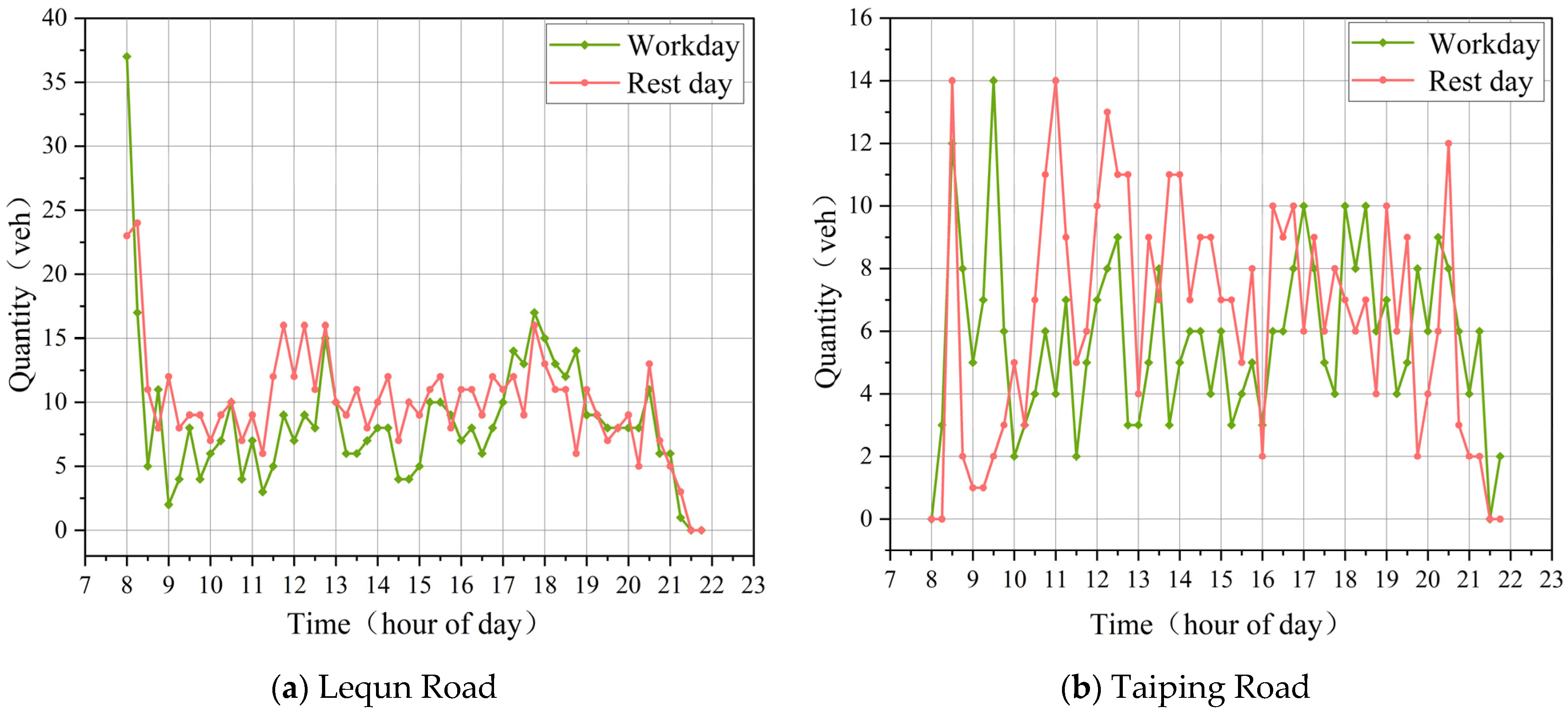
In general, demand is higher on weekends or holidays than on weekdays, probably because people generally have more activities on weekends or holidays. However, the demand in commercial or office areas may be different. It can be seen from Figure 3 that the parking demand on Lequn Road is higher than that on weekdays in all hours on rest days, but the difference is not extremely significant. The demand is obviously higher in the morning hours on weekdays than on rest days, which may be due to the fact that there is a hospital near Lequn Road, and the attraction of a hospital for parking is relatively more balanced both during the weekdays and on weekends, while the morning peak on Taiping Road on rest days lasts shorter than weekdays and starts later than weekdays. As there are many restaurants and other stores around Taiping Road, as well as kindergartens, the parking demand on rest days is basically higher than that on weekdays, except for the hours around 8:00 a.m. and 17:00 p.m. This may be due to the fact that children are picked up and dropped off at kindergartens in the morning and evening on weekdays, but not on weekends. More parking demand occurs on rest days usually because people may always have more activities during the rest time.
(3)
Time Factors
The time feature vector f t D primarily indicates which daily parking period that the time interval t falls within. Since the parking demand of the whole block is aggregated as the number of parking inflows within 15 min, the time should be encoded into an ordered sequence of integers, again in 15-min increments. The parking period is obtained as 8:00–22:00 per day, so the sequence is defined starting from 8:00. For example, the interval of 8:00–8:15 is set to 1, while the interval of 14:00–14:15 is set to 25, i.e., 14 8 × 4 + 1 . The feature of time is regular and has a significant impact on the performance of demand, which will have different performance at different times, including the peak and flat performance of parking demand, so grasping this regular feature will help the effective prediction of parking demand.
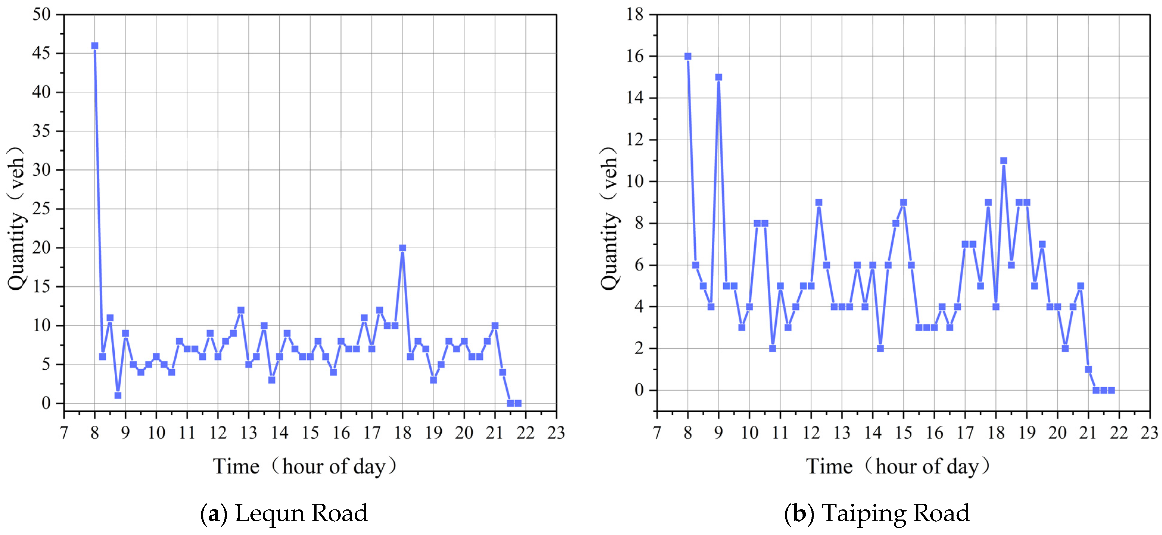
Generally speaking, the peak hours of parking demand occur in the morning from 8:00–9:00 and in the evening from 18:00–19:00, as people generally choose to travel during such hours, such as commuting to and from work and picking up and dropping off children from school. Of course, such a trend may vary depending on the properties of the block. From Figure 4, it can be found that the parking demand of Lequn Road mainly has two peak hours in the morning and evening, which is in line with the commuting hours of commuting to and from work or school. On the other hand, Taiping Road has small peaks in the morning, midday, and evening, and significant difference does not occur in the demand at different times of the day. It is mainly related to the properties of the road section itself, because the road section is mainly surrounded by food service facilities.

Model Design

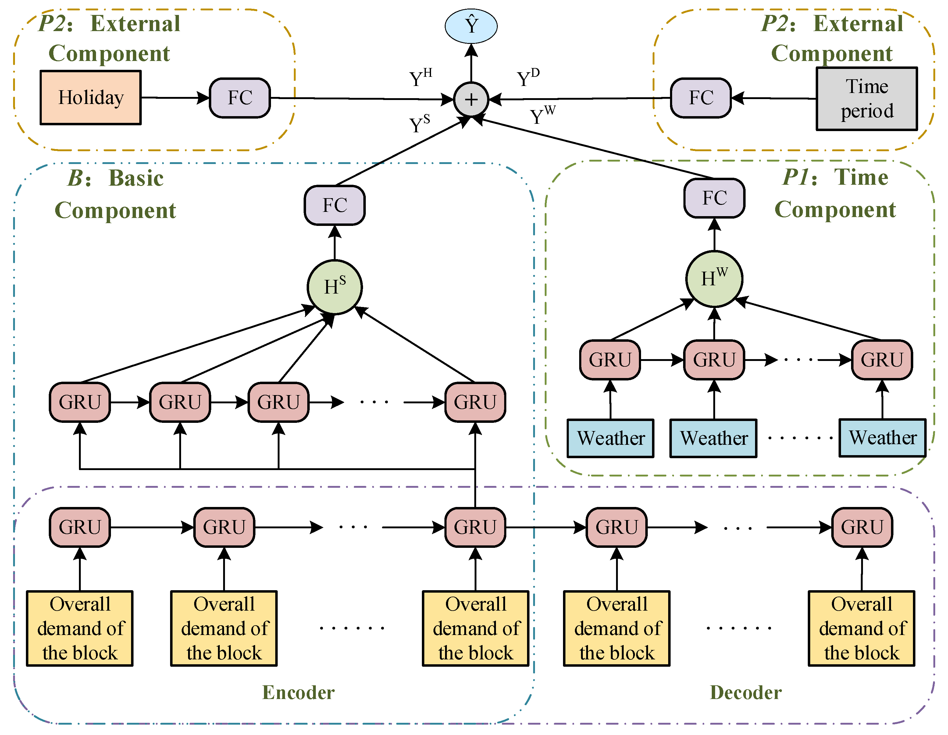
As described in the previous section, the features that have an impact on the demand are different, so their data formats are different. Therefore, in the procession of a model’s construction, two different types of components are used to model demand data and external feature data separately, as shown in Figure 5. The model mainly includes B: Base Components, which use the encoder–decoder structural framework to extract the features and patterns present in the historical parking demand data; P1: Temporal Components, which use gated recurrent units (GRU) to capture the temporal correlation based on the time-variant weather features which is related to the historical parking demand of the block; P2: External Components, where holiday features as well as time period features are modeled separately using fully connected neural networks.
First, in order to expand the valid data and improve the accuracy of the data at the same time, the value of one point is no longer limited to a certain point, but is expanded to an interval containing this point, and the entire interval is continuously moved backwards in certain units. Eventually, these intervals are used for subsequent judgments, which is called a sliding window that enables the time series to be framed according to a specified unit length, so that the statistical indicators within the frame can be calculated.
B: Basic Component. By the method of sliding window, the historical parking demand quantity sequence [ q 1 , q 2 , , q T ] obtained at 15-min intervals is divided into a quantity sequence { [ q t l + 1 , q t l + 2 , , q t ]   t = l , l + 1 , , T } of regional historical parking demand of length l. Prior to fitting the prediction model, the historical parking demand sequence of the whole block is fed into an encoder–decoder framework consisting of a two-layer GRU network to capture the inherent patterns that the sequence itself has. After pre-training the encoder–decoder, it can be considered as an automatic feature extractor. The last GRU unit state of the encoder is extracted and is fed into the prediction network later as a learning embedding for further prediction. The embedding result is input to the prediction network to obtain the output H S = { [ h t l + 1 S , h t l + 2 S , , h t S ]   t = l , l + 1 , , T } of the hidden layer unit, and then the hidden unit H S is input to the fully connected layer (FC) to output the demand quantity inflow Y S for the target time interval.
P1: Time Component. Similarly, a GRU network is used to capture the temporal correlation of weather features, and the model is similar to the construction of the demand quantity series prediction network. The weather feature sequences obtained by sliding time windows are input into the GRU network to output the hidden unit H W , after which the hidden unit H W is input to the fully connected layer (FC), and finally the inflow Y W for the target time interval is output.
P2: External Components. For the features with low temporal granularity, like holiday and time period features, the time units should be reduced to the same units as the time interval set in the time component firstly, and then the fully connected layer (FC) is selected to capture the key factors that can have an impact on the whole network. The holiday inflow Y H and the time period inflow Y D of the target time interval are outputted through fully connected layers, respectively.
Finally, the target time interval inflows Y S , Y W , Y H , and Y D obtained from each component are combined to derive the quantity Y ^ of overall parking demand prediction for the target time interval, which is defined as:
Y ^ = tanh ( Y S + Y W + Y H + Y D )

3.2.2. Parking Demand Distribution Prediction within Block

This section describes how to predict the parking demand distribution in the block at the ( T + 1 ) -th time interval. It is combined with the overall parking demand forecast for the block to obtain the final parking demand prediction for each section.

Feature Analysis

The main characteristics that influence the distribution of parking demand between sections within a block are time-invariant characteristics, which can also be understood as spatial association characteristics between different sections, i.e., physical location as well as semantic function. These two types of features are representations of the interactions within the block and have a considerable influence on the distribution of demand for each road segment within the whole block.
(1)
Physical Location
Define the center coordinates of each section as its specific physical location coordinates. Usually, two relatively close parking areas will have a high level of similarity in demand. In most cases, when a driver finds that there are no available spaces in the target parking section, he or she will cruise from the current section to the surrounding sections in close proximity to find an available parking space.
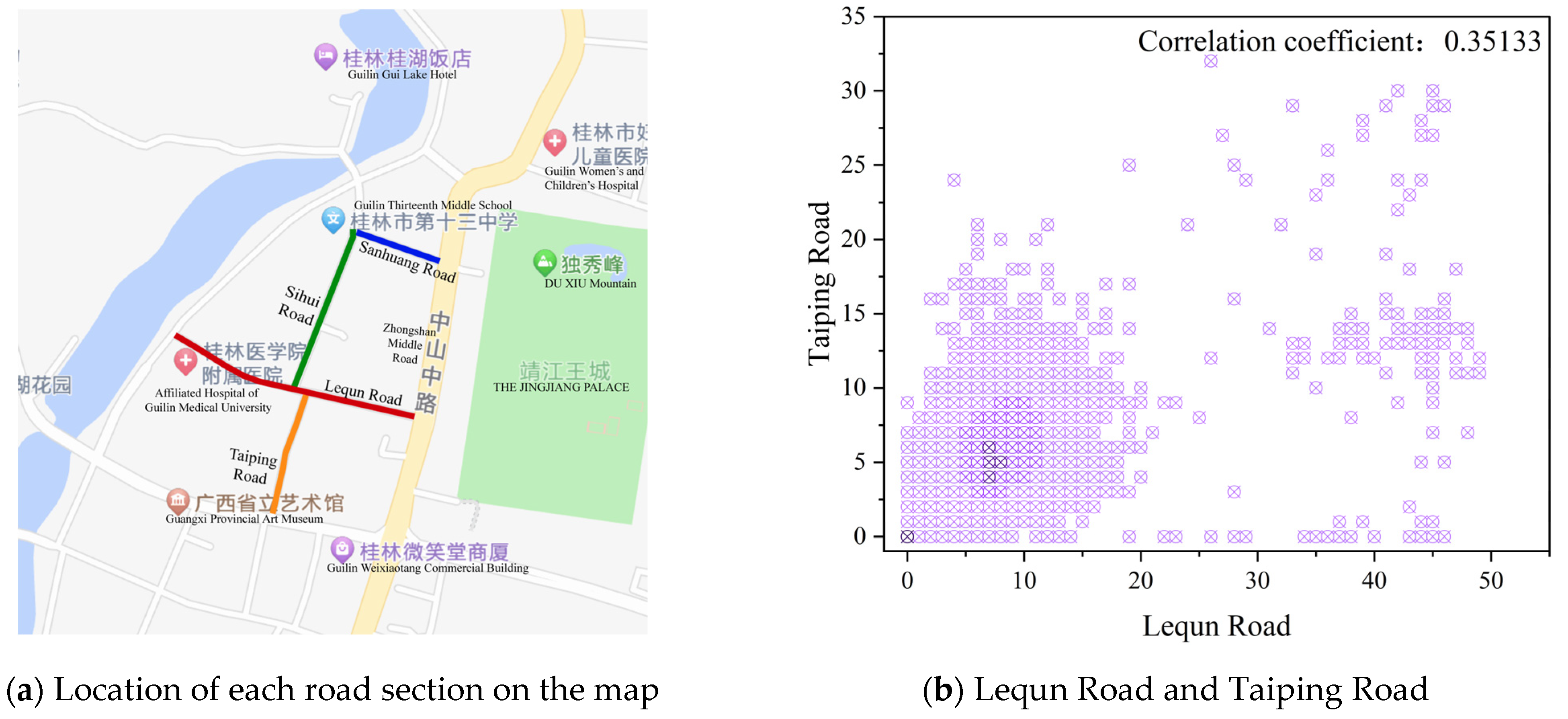
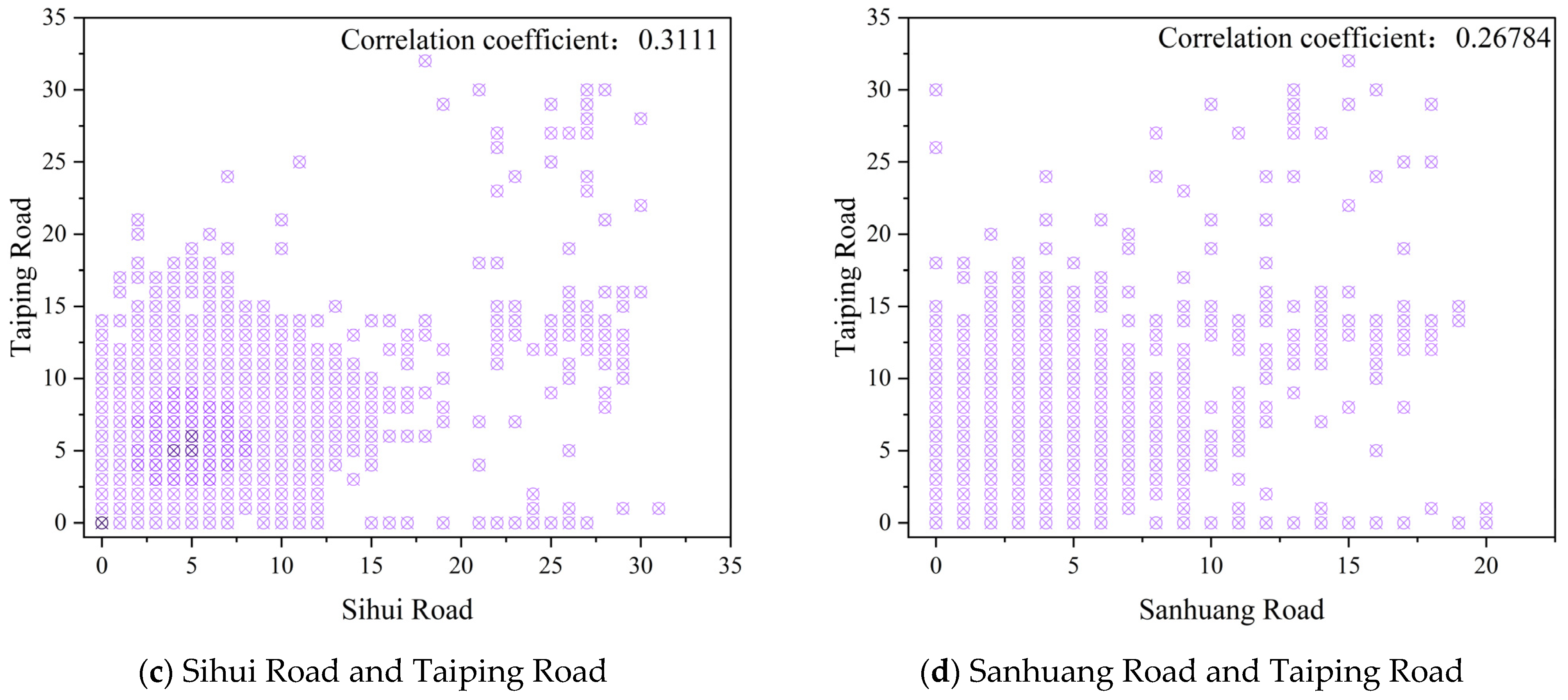
Taking the four on-street parking sections in Xiufeng District of Guilin—Sanhuang Road, Sihui Road, Lequn Road, and Taiping Road—as examples, the relative positions among several road sections can be observed through Figure 6a. In terms of physical location, the physical distance gradually increases between Taiping Road and Lequn Road, Sihui Road and Sanhuang Road, while by observing the two-dimensional scatter plot between the road sections, it can be seen that as the physical distance between the two road sections increases, the correlation between their parking demand decreases. It can also be observed that the correlation between two road sections that are very close in physical distance does not produce a very large gap with those that exist at a certain distance. It can be seen that the correlation between Lequn Road and Sanhuang Road, which are not physically located next to each other, even exceeds the correlation between Lequn Road and Taiping Road by quite a bit. Therefore, it can be inferred that there may be other types of features that also have an impact on the correlation between the road sections.
(2)
Semantic Function
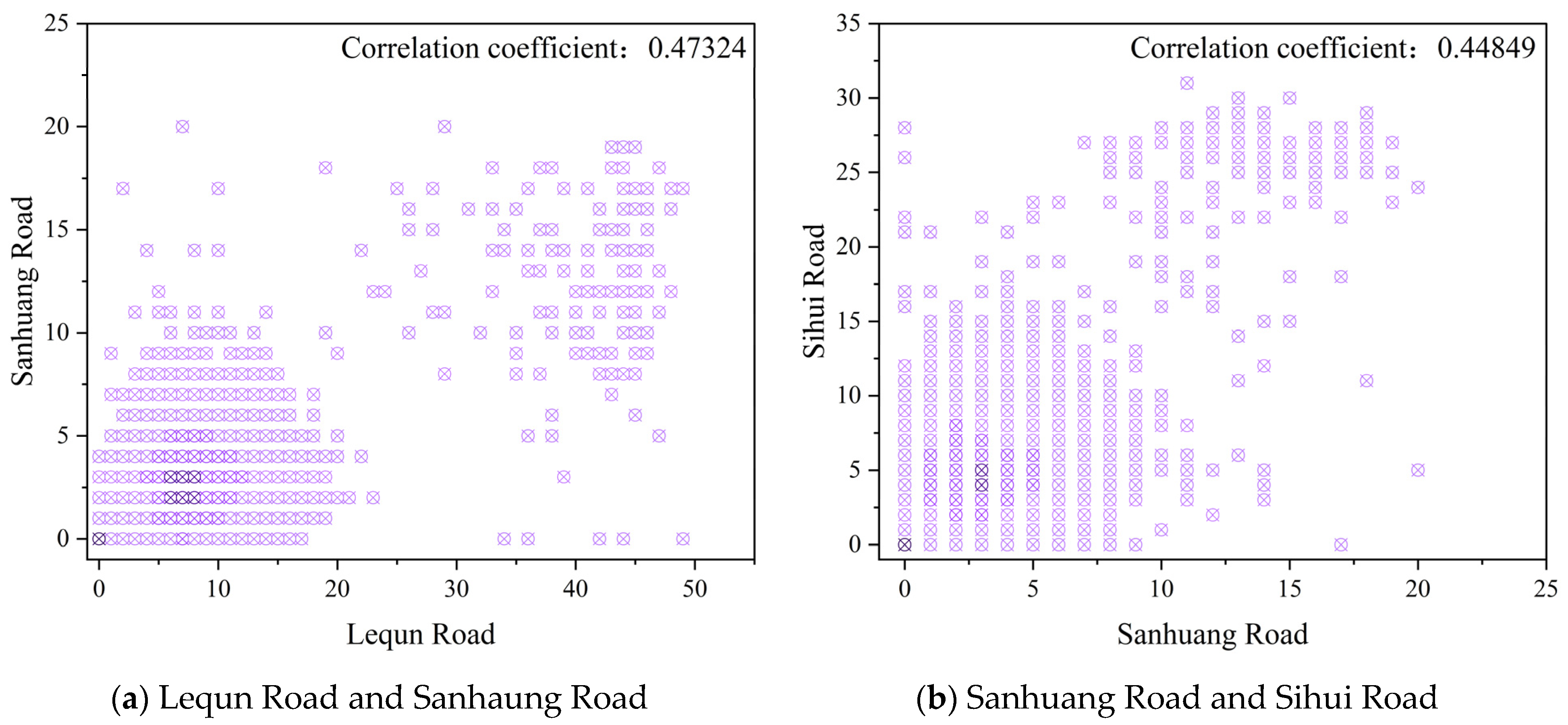
The semantic function of each parking section can be characterized by a vector of points of interest (POI), in which the dimension is the number of categories of points of interest (POI), while each element is represented as the result of combining the number of POIs of each type within a specific area around the section and the walking distance between each POI and the section. The specific combination will be explained in detail in the model design section in ‘Model Design’ part. Usually, two blocks with similar semantic functions may have related inflows. The detailed calculation results of the semantic functional similarity by Equations (3) and (4) are shown in Table 1.
As can be seen from Figure 7, the correlation between Sanhuang Road and Lequn Road is slightly higher than that between Sanhuang Road and Sihui Road, probably because they have more similar semantic functions. Although in terms of physical distance, Sihui Road is closer to Sanhuang Road than Lequn Road, the semantic similarity between Sanhuang Road and Lequn Road is higher than that of Sihui Road according to the results of the semantic function calculation. Therefore, a higher correlation is presented between Sanhuang Road and Lequn Road, which is also proved by the results of the semantic function calculation.

Model Design

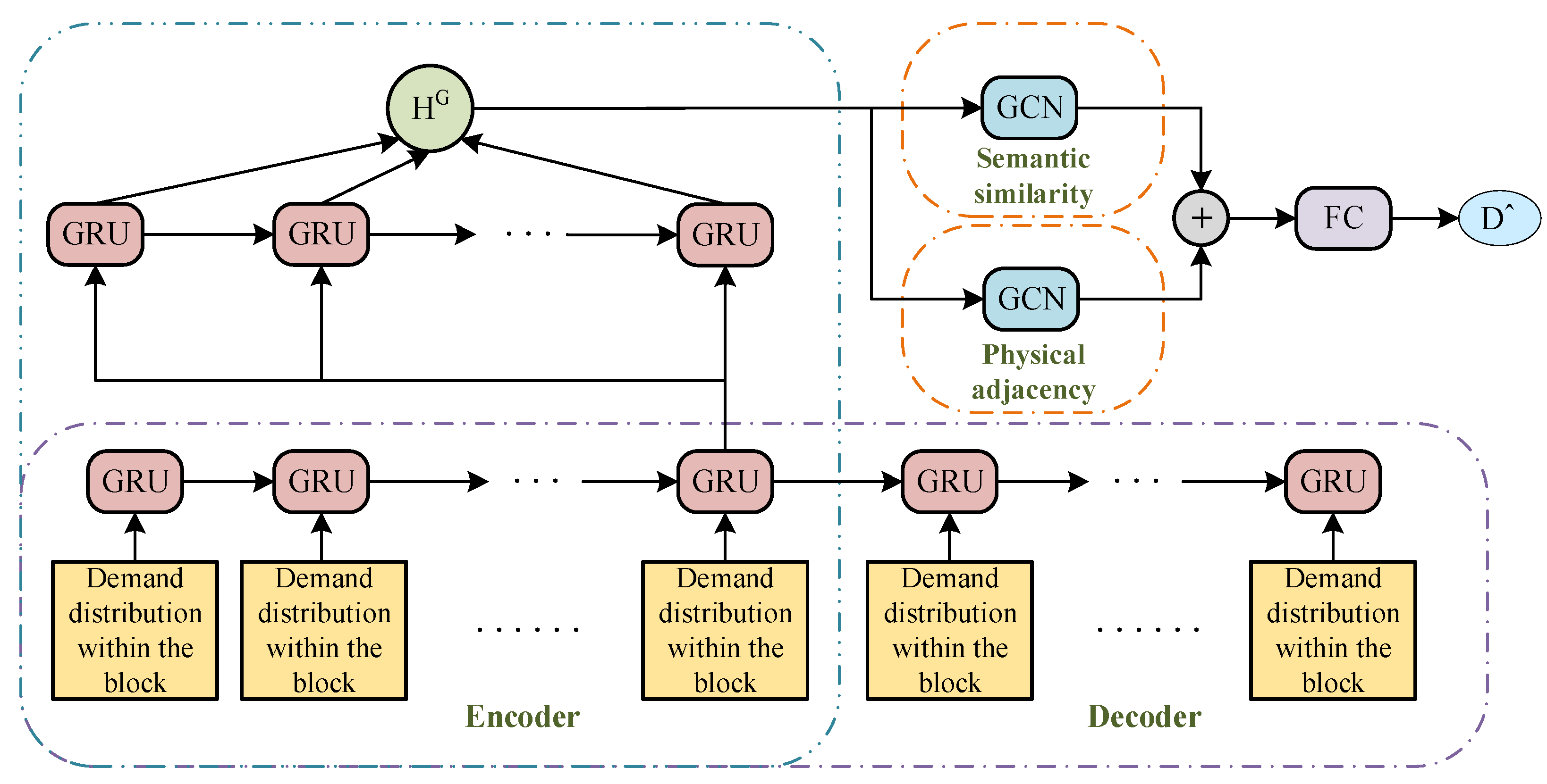
Based on the factors affecting the distribution of parking demand within a region in the previous section, and considering the time-invariant property that both factors are capturing internal correlations within the block, a demand distribution prediction model based on two types of graph structures is designed, as shown in Figure 8. The demand distribution embedding results extracted by the encoder–decoder are fed into a distribution prediction network combining gated recurrent unit network (GRU) and graph convolution (GCN), which is to capture the spatial correlation between road segments within the block. The two graph structures are represented by the physical proximity and semantic similarity among the road segments in the block, respectively, where nodes denote road segments in a block and edges denote connectivity relationships between road segments.
First, similar to the prediction of the overall parking demand of the block in the previous chapter, an encoder–decoder framework consisting of a two-layer GRU network is designed to capture the inherent patterns and correlations between the demand distribution sequences themselves. Its last state of GRU unit is extracted as a learning embedding input to the network that follows. The predictive body structure of the demand distribution starts with the GRU, which accepts the embedding results from the encoder–decoder output as input and outputs the hidden layer unit H G , i = { [ h t l + 1 d , i , h t l + 2 d , i , , h t d , i ]   t = l , l + 1 , , T } . H G represents the hidden states [ H G , 1 , H G , 2 , , H G ,   V ] of all nodes in the graph, and these states are fed into the next graph convolution network. Typically, in a given graph G = ( V , A ) , the adjacency matrix is represented by A   V ×   V and its elements represent the connections between the nodes in the graph. Graph convolution can delicately extract the corresponding features from graph data and, in particular, introduces a well-performing hierarchical propagation rule for neural network models of non-Euclidean data [36]. The main building process for both types of graph structures is as follows.
Physical adjacency graph  G P = ( V , A P ) . The physical proximity relationship is constructed by the inverse of the driving distance between two nodes in the graph, the further the driving distance, the weaker the proximity relationship. The adjacency matrix A P can be expressed as follows [37]:
A P , i j = 1 i j
where i j denotes the driving distance between two nodes v i V ,   v j V in the graph.
Semantic similarity graph  G Y = ( V , A Y ) . The graph is constructed by the cosine similarity of the semantic functions between two nodes in the graph. The closer the similarity is to 1, the more similar the semantic functions are. The adjacency matrix A Y can be expressed as follows [37]:
A Y , i j = y i y j y i y j
where y i , y j denotes the semantic function vector of the two nodes v i V ,   v j V in the graph.
The semantic function vector is defined by the combination of the number of each type of POI within a specific area around each node and its corresponding walking distance from the node. The semantic function vector y i = [ y i , 1 , y i , 2 , , y i , k ] for each node in the figure is composed of k POI categories. y i , c ,     c k in the vector represents the value of the element calculated for the c-th POI category, and the value of the element is expressed as the product of the average walking distance from all points to the node in each category of POI and the proportion of that category of POI in the overall. The specific definition is as follows:
y i , c = o = 1 n c b i o n c × n c c = 1 k n c = o = 1 n c b i o c = 1 k n c
where n c denotes the number of POIs of the c-th class owned in a specific area around node i, and b i o denotes the walking distance between the o-th POI point in the class and node i.
The propagation between layers of a graph convolutional neural network is as follows [36]:
H l + 1 G = σ ( D ˜ 1 2 A ˜ D ˜ 1 2 H l G   W l )
where H l G and H l + 1 G denote the node characteristics of layer l and layer l + 1, respectively, and W l denotes the weight parameter of layer l. Meanwhile, the adjacency matrix A is normalized, and finally, the symmetric normalized Laplacian matrix in Equation (5) [36].
Finally, the result of the graph convolution is output to the fully connected layer (FC) to finally obtain the demand distribution inflow D ^ = [ d ^ 1 , d ^ 2 , , d ^ V ] for the target time interval.

3.2.3. Fusion

Based on the output of Section 3.2.1 and Section 3.2.2, the overall parking demand Y ^ is directly combined with the internal parking demand distribution D ^ to finally obtain the parking demand for each section of the region for the target time interval.
Q ^ = [ q ^ 1 , q ^ 2 , , q ^   V ] = Y ^ × [ d ^ 1 , d ^ 2 , , d ^   V ] = Y ^ × D ^

4. Experiments

In this section, we conduct experiments to evaluate the parking demand prediction model proposed above. The data used in this paper are derived from real on-street parking business order data in the central city of Guilin, China, spanning the period from 30 November 2020 to 30 April 2021. In addition, we design ablation experiments to compare the effects of the models for each feature.

4.1. Datasets

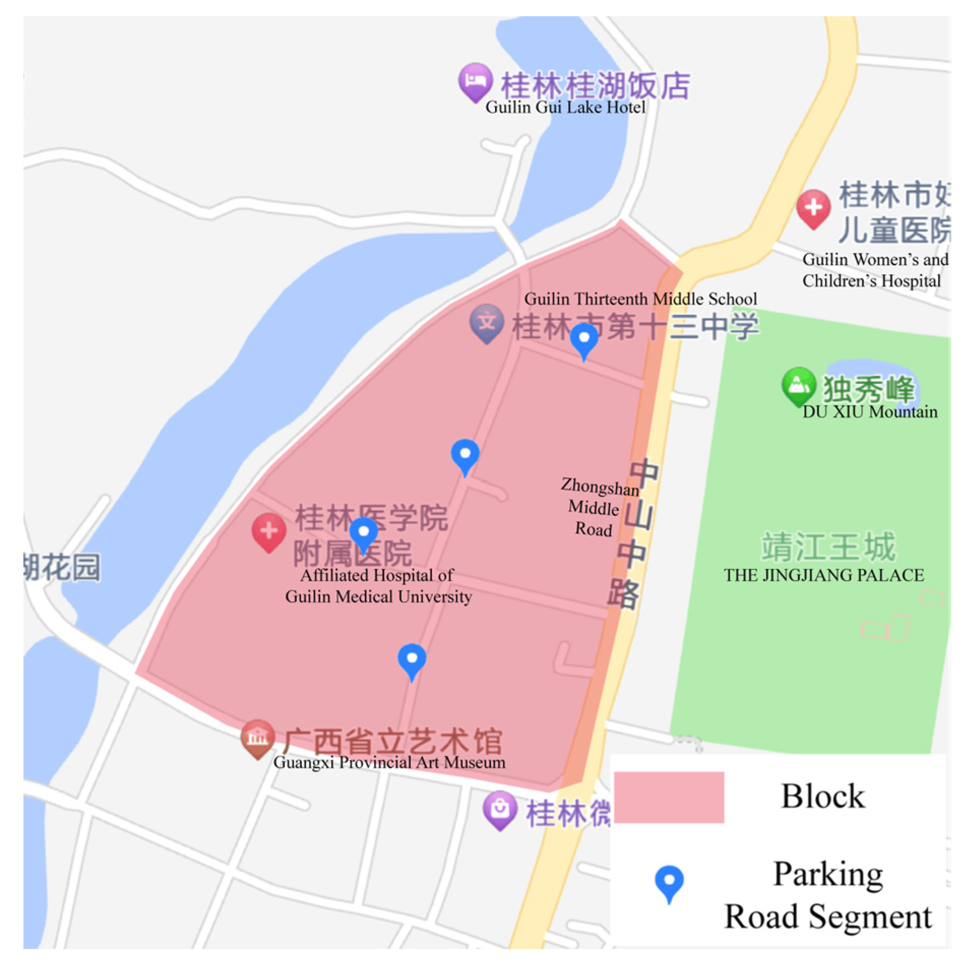
The main basis of the study block division is the city’s main roads. For example, Figure 9 shows the division representation of a block in Xiufeng District, Guilin. By processing and cleaning the raw data for outliers and missing values, a total of 192,421 historical parking order records were obtained. The parking business orders mainly contain information such as the specific name of the road section parked in by the parker, the specific time of arrival and departure, and the number of the parking space. Using 15 min as the time interval, the data are aggregated into the number of parking inflow per 15 min by different road sections to obtain the number of parking demand in each daily time period from 30 November 2020 to 30 April 2021 for different road sections. Take the block shown in Figure 9 as an example. According to our statistics, the average daily parking demand in this block is about 1300 vehicles. The average daily parking demand on Lequn Road is about 473 cars and on Taiping Road is about 341 cars. The number of parking spaces in several sections of the block are listed in Table 2.
In the model training process, the historical parking demand data for the entire region from 30 November 2020 to 31 March 2021 are used as the data for training the overall parking demand prediction model, and the data from 1 April 2021 to 30 April 2021 are used as the test data. Also, the amount of parking inflow for each road segment as a percentage distribution of the entire block is used as data for the internal parking demand distribution. Similarly, the distribution data from 30 November 2020 to 31 March 2021 is used as the training data for the internal parking demand distribution prediction model, and the distribution data from 1 April 2021 to 30 April 2021 is used as the test data.
In addition, the use of multiple sources of external data has been added to enable the model to capture more features.
(1)
Hour-by-hour weather data from 30 November 2020 to 30 April 2021 for Guilin. Precipitation, wind speed, visibility, and temperature data are screened from it. Data are obtained from the NCEI National Environmental Data website.
(2)
The specific scheduling of actual weekdays and holidays is obtained from the holiday scheduling notice issued by the General Office of the State Council of the People’s Republic of China.
(3)
Driving path planning and driving distances between different road sections in the region, with data from the Gaode Open Platform.
(4)
POI data of different categories within the specific area around each road section, with 23 categories in total, with data from the Gaode Open Platform.
(5)
The walking path planning and walking distance between each road section and each POI in the specific area around it, with data from Gaode Open Platform.
It is important to note that the data mentioned above that needs to be accessed through the Gaode Open Platform requires the use of programming. In addition, it is necessary to apply for the relevant application on the platform and use it only after obtaining the key.

4.2. Experimental Settings

4.2.1. Evaluation Metrics

For the prediction results, root mean square error (RMSE) and mean absolute error (MAE) are selected as the evaluation indexes for the roadway parking demand prediction, and the smaller the error obtained, the better the performance of the model.
Equations (7) and (8) give the calculation of RMSE and MAE [2]:
R M S E = 1 n i = 1 n E i 2 = 1 n i = 1 n ( q i q ^ i ) 2
M A E = 1 n i = 1 n E i = 1 n i = 1 n q i q ^ i
where E i denotes the absolute error between the i-th actual value and the predicted value, q i denotes the actual parking demand value of the i-th road section, and q ^ i denotes the predicted value of the i-th road section. Both the value of RMSE and MAE are absolute indicators. When comparing the prediction performance of different models for the same target, RMSE and MAE are considered to be the most relevant evaluation metrics.

4.2.2. Baselines and Details

The modeling approach presented above is compared with the following baselines that can be used for parking demand prediction: (1) Historical Average (HA); (2) Auto-Regressive Integrated Moving Average (ARIMA); (3) Long Short-Term Memory Network (LSTM); (4) Gated Recurrent Unit Neural Network (GRU); (5) GCN+GRU, a prediction method that combines graph convolutional network and gated recurrent unit network, which can extract the information from the graph structure to improve the prediction performance. Information from the graph structure is used to improve the performance of the prediction, but only where the effect from the physical distance graph is considered.
In the comparison with the above baseline, the focus of the entire process is always on the road segments and does not combine the block with its internal distribution. The basic idea of “combining the overall parking demand and internal demand distribution of the block” used in the previous section is named “B&D”, and its significance will be demonstrated by adding this method to the above baseline and comparing it with the non-added baseline. In other words, there is a combination of the joined methods: HA+B&D, ARIMA+B&D, LSTM+B&D, GRU+B&D, GCN+GRU+B&D.
All models of deep learning networks are built and implemented in Python 3.9.7, TensorFlow 2.8.0, and Keras 2.8.0 under Anaconda platform, optimized with Adam optimizer, and with an early stopping mechanism set to prevent overfitting of the models.
The following are the main model design details for the comparison baselines. In HA, the average of the demand for the same time period of the past 56 days is used to achieve the prediction of the next day’s values for the same time interval. For LSTM, GRU, and GCN+GRU, 56 sets of historical observations are inputted into the model for the next forecast after processing the data using a sliding window, i.e., using the historical observations of the past day for the next 15-min demand forecast. In the prediction, both LSTM and GRU use two-layer networks and choose RELU as the activation function, while GCN+GRU use two-layer networks and also use RELU activation function. In addition, the model in this paper adds another GCN network to GCN+GRU to further capture the semantic correlation between nodes which use the same parameters as before.
Similarly, we design ablation experiments considering different features on the basis of the above experimental settings. The relevant features in the overall demand prediction module and the internal distribution prediction module of the previous model are excluded, respectively. The model performance in the ablation experiment is then evaluated using the error evaluation index mentioned above to assess the impact of each feature in the model on the final prediction results. The specific setup of the ablation experiment is as follows:
(1)
Only the P1 component of the overall prediction module in the model is excluded.
(2)
Only the P2 component of the overall prediction module in the model is excluded.
(3)
The P1 component and the P2 component of the overall prediction module in the model are also excluded.
(4)
Only physical adjacency features of the internal distribution prediction module are excluded.
(5)
Only the semantic functional similarity relationship features of the internal distribution prediction module are excluded.

4.3. Experimental Results

4.3.1. Results Compared with Baselines

Table 3 shows the results of this paper’s model and other different baseline models for road segment demand prediction. Based on the comparison of the results of each model approach in the table, it is easy to see that the model in this paper works better compared to the traditional model. This is mainly because the modules of the model combine to fully capture the characteristics of parking demand from both temporal and spatial perspectives. These features are not only the relevant features of the road sections themselves, but also the correlation features between the road sections.
From the results, it can be calculated that the prediction results of our proposed model improve by an average of 28.8% in the metric of RMSE compared to the baselines. Among them, the average improvement is 36.57% compared to the baselines without using “B&D” structure. In contrast, for the baselines that used “B&D”, the average improvement is 21.13%. As for the performance of the MAE, our model improves by 31.70% and 16.14%, respectively, compared to the baselines before and after using the structure “B&D”, and the overall average improvement is 23.92%. Although such an error result may not seem large in numerical terms, the impact of such a value is quite significant for on-street parking, because in our data, the number of parking spaces in the road sections are not large as can be seen in Table 2. On the basis of such a number of parking spaces, it is possible to obtain an improvement in the error value of about 2, which we think is meaningful for some subsequent studies based on the prediction results.
The observation of the comparison of the results reveals that the historical averaging (HA) as well as the moving average autoregressive (ARIMA) models do not perform well on the data set. This is because the nature of both HA and ARIMA models for capturing data are limited to linear relationships, while it is clear that the parking demand exhibits significant nonlinearity in its characteristics. At the same time, the ARIMA model relies heavily on the goodness of the fixed-order results and only fits the series itself without considering the relevant influencing factors of parking demand. The LSTM and GRU, as neural network models with prediction functions, can capture the characteristics of the sequence in the temporal dimension, but not in the spatial dimension, which causes a certain degree of error in their prediction results. Moreover, after adding GCN based on a physical location relationship map, the prediction ability of the model is significantly improved.
The results in the bottom half of Table 3 also show that the forecast structure of “B&D” allows a more comprehensive and detailed analysis of demand-related influences, capturing the impact of different characteristics from different perspectives, and thus achieving more accurate model demand forecasts. The data in the table also shows that the prediction results of all models are better than those without using the “B&D” infrastructure. In particular, the LSTM and GRU have significantly improved before and after the use. This indicates that the prediction structure we designed has improved the prediction results by combining the overall and internal information about the parking area and incorporating this information into the prediction model. In addition, this structure improves the prediction effect more for LSTM and GRU, probably because these two models themselves can already capture the time-dimensional features in the sequence. Moreover, if the model is then put into the prediction structure that combines the whole and the interior, then the prediction model will absorb some spatial information brought by this structure, and thus achieve more accurate prediction results. In general, combining overall demand and internal distribution considerations to forecast demand in parking areas will help to capture the correlation between demand and improve the accuracy of model forecasts.
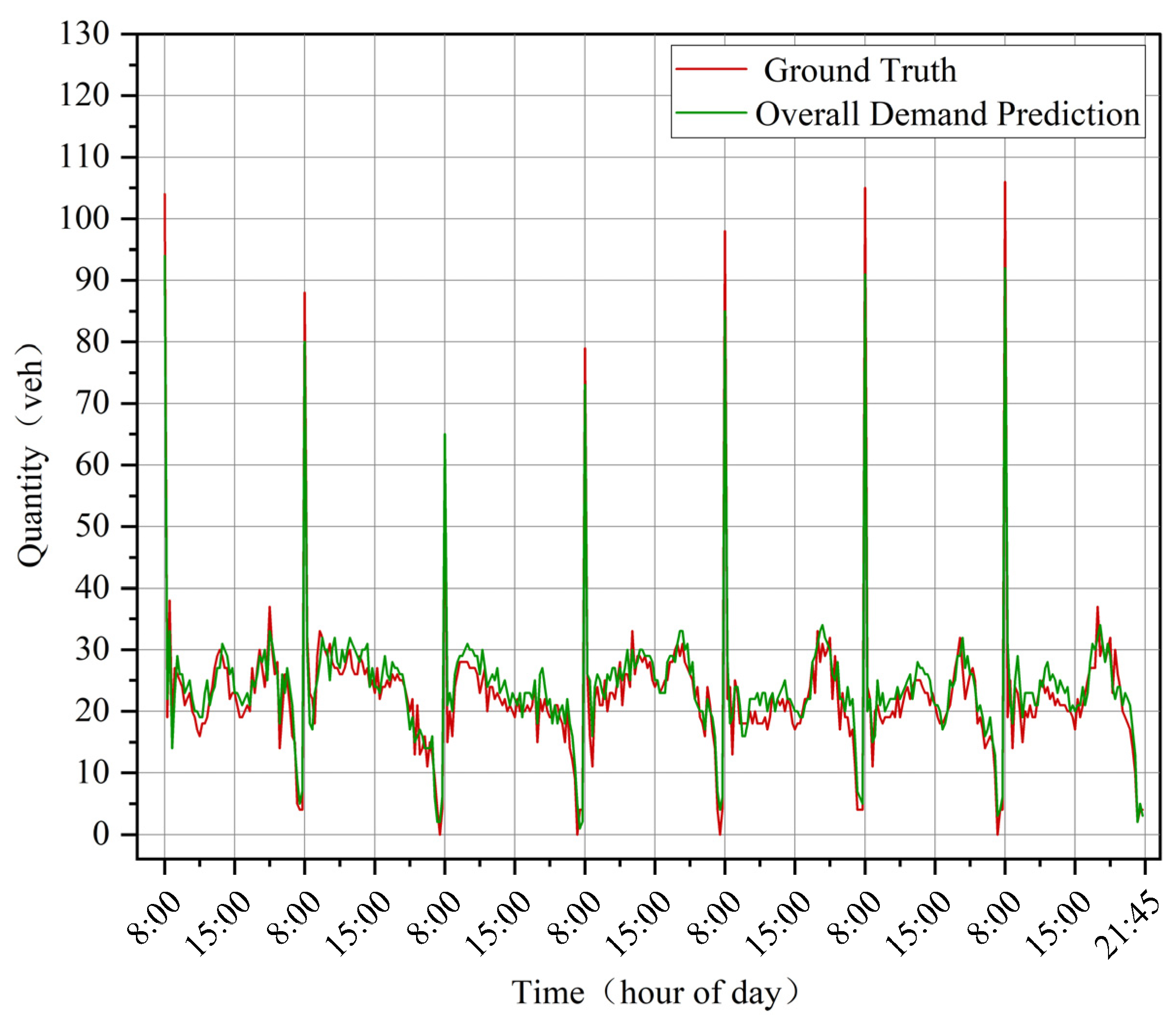
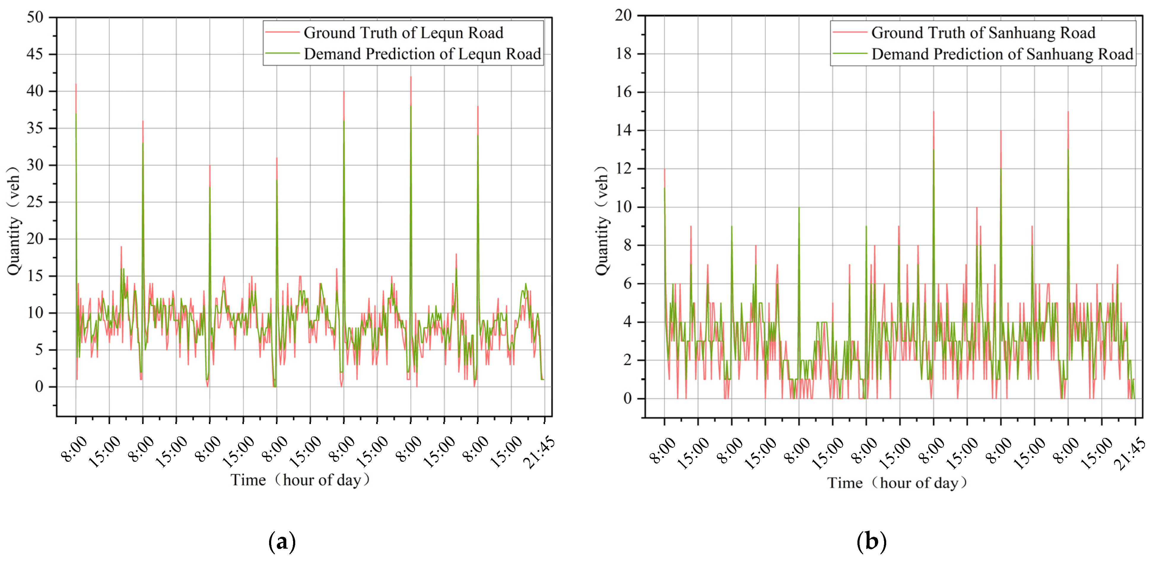
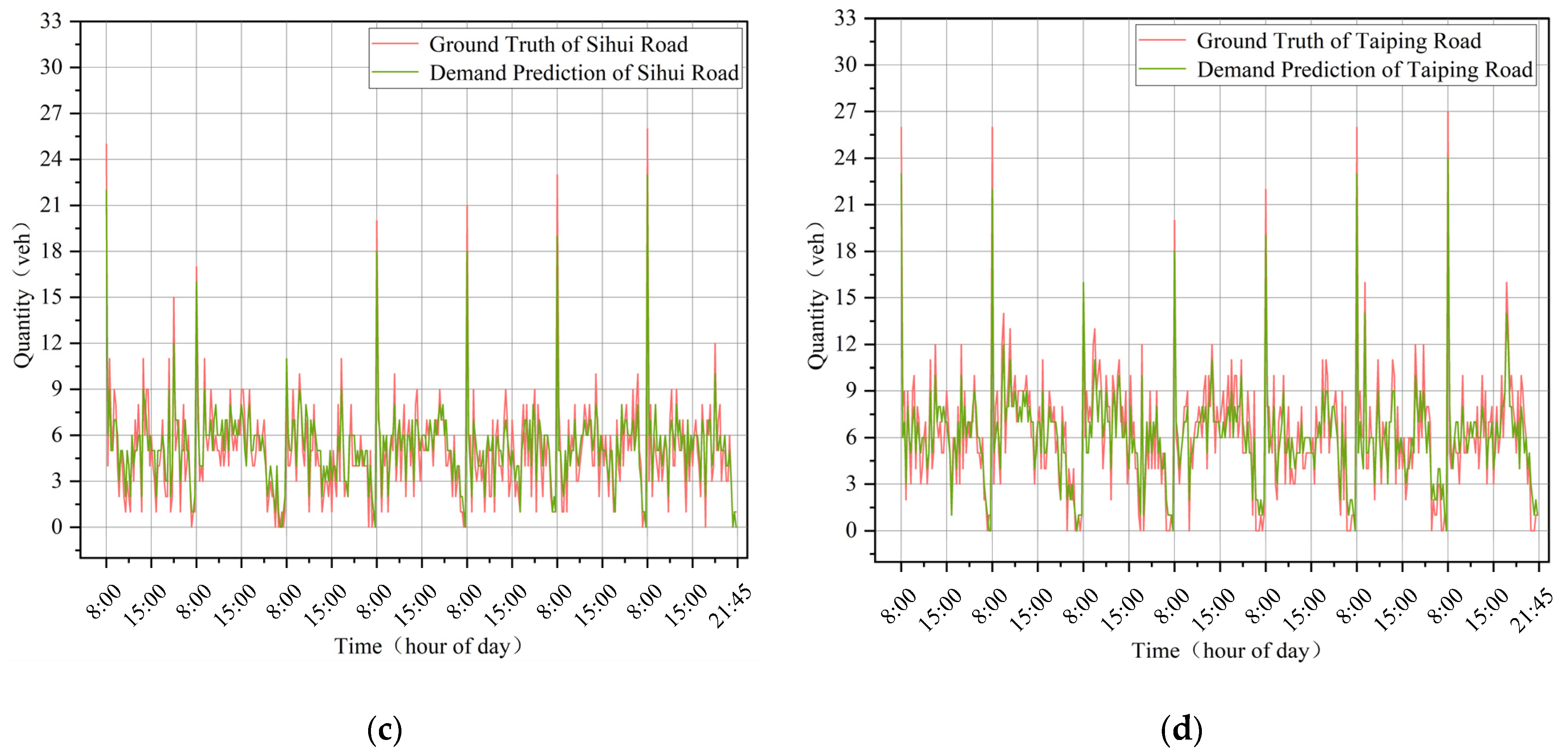
Figure 10 shows the results of the overall demand forecast for one week from our model compared to the original demand data. Figure 11 shows the results of the model’s final one-week parking zone forecast results compared to the original parking zone demand. It can be clearly seen from these figures that our model captures better the smaller range of variations in the overall parking demand presented during the day. Additionally, the fitting of the maximum value of the daily morning peak can be conducted relatively accurately.
Figure 12 shows the comparison of the results of various types of neural network baselines with the models proposed in this paper for each day of prediction. Due to the large amount of data and the density of the data, we have performed only one day of prediction results of Lequn Road for comparison in Figure 12. It can be seen that although these baseline models can capture the fluctuation of demand to some extent, they are not sensitive to some sudden fluctuations or abrupt changes caused by special time, and they can often only fit the general tendency, but cannot obtain more accurate prediction results.

4.3.2. Ablation Experiments with Different Components

The results of the experiment are shown in Table 4, where the absence of any part of the model’s characteristics has an impact on the evaluation indicators. Similarly, the results of this ablation experiment can be inferred by considering the impact of weather, holiday, and time of day features on demand prediction.
Figure 13 shows the performance of our model on parking demand prediction under these ablation experiment settings. Due to the large amount of data and the density of the data, we have performed only one day of prediction results of Lequn Road for comparison in Figure 13.
It can be seen that characteristics that have an impact on the overall demand, such as weather and holidays, have an impact on the final prediction accuracy of the demand prediction model proposed in this paper. Second, the impact of internal distribution-related features on the model will be relatively more significant than the impact caused by overall demand-related features on demand forecasts. The results of both the figure and the table indicate that the exclusion of internal distribution-related features affects, to some extent, the model’s ability to capture more intensive changes in demand, especially small fluctuations. For example, in Figure 13, there are small fluctuations in the actual values around 9:00 a.m. It is clear that the model with the semantic functional correlation feature excluded does not capture the small fluctuations in this time period clearly enough, and the predicted results are relatively flat. The model with other features excluded captures such changes, but it is not accurate enough and the error is relatively larger. The model that combines all the features does not capture the relatively abnormal sudden changes like the morning peak accurately enough. This is another aspect that proves that considering the correlation between the parking area itself and the surrounding parking area, including the physical location relationship as well as the semantic functional correlation, has an impact on the demand prediction. The model proposed in this paper incorporates these features to capture these correlations better to some extent and achieves a better representation of the model for these characteristic factors.

5. Conclusions

In order to further provide accurate demand prediction for on-street parking, reduce unnecessary cruising on urban road sections, improve parking efficiency, and at the same time enhance the convenience of drivers’ parking, this paper proposes a prediction model that integrates the use of deep learning network structures such as encoder–decoder, GCN, and GRU. The model is made from two perspectives, including the overall demand and internal distribution of the block, to richly and meticulously capture the impact of different features and finally achieve accurate prediction of parking demand on road sections.
During the construction of the demand prediction model, in addition to the historical demand sequence part, various types of features including weather, holidays, and time periods are mainly used. The graph structure is especially used to capture the correlation features between road sections and their surroundings, and a demand prediction model with more comprehensive coverage features is obtained. In this paper, the model is evaluated with a 5-month real parking dataset in the central city of Guilin. The results show that the model proposed in this paper outperforms other baselines by about 25% on average in terms of metrics. In addition, the use of the structure of “combining the overall demand and internal demand distribution of the block” for fitting the demand has obvious advantages. Additionally, an ablation experiment is designed to evaluate the importance of different features in the model. From the results, it can be seen that the absence of any feature in the model has a significant impact on the results. In other words, the inclusion of each feature has an impact on improving the prediction performance of the model.
From the application point of view, the demand prediction model proposed in this paper can be directly connected with other guidance or management systems to a large extent. Current advanced urban intelligent parking management systems are in need of clear parking demand prediction results to provide appropriate guidance to drivers and parking managers. For example, providing the driver with the future parking status of the destination for him to decide the final destination of driving, etc., can largely avoid unnecessary cruising behavior. Parking managers can also use the predicted parking situation to make dynamic adjustments to parking fees in advance to improve parking demand and increase the efficiency of their operations. The application of accurate demand prediction results to the above-mentioned work will also be a very practical task. We will also further study the application of parking demand prediction in the decision scheme of parking guidance.

Author Contributions

Conceptualization, T.W. and Q.Y.; methodology, S.L.; software, S.L.; validation, T.W.; formal analysis, S.L.; investigation, S.L.; resources, X.T.; data curation, S.L.; writing—original draft preparation, S.L.; writing—review and editing, T.W. and Q.Y.; supervision, W.L. and J.C.; funding acquisition, T.W. All authors have read and agreed to the published version of the manuscript.

Funding

This research was funded by the Fund for National Natural Science Foundation of China (52262047), Guangxi Science and Technology Base and Talent Special Project (AD20159035), Guilin Key Research and Development Program (20210214-1), and the National Natural Science Foundation of China (61963011, 71971059).

Institutional Review Board Statement

Not applicable.

Informed Consent Statement

Not applicable.

Data Availability Statement

The data presented in this study are available on request from the corresponding author. The primary data of historical parking business orders are not publicly available due to the need for subsequent related work. The rest of the open source data are available according to the annotation in the text. Weather data are available at https://www.ncei.noaa.gov/access/search/data-search/daily-summaries, accessed on 25 August 2022. The specific scheduling of actual weekdays and holidays is available at http://www.gov.cn/fuwu/2020-11/25/content_5564533.htm, accessed on 17 April 2022. Driving path planning, walking path planning, and POI data are available at https://console.amap.com/dev/index, accessed on 10 May 2022.

Conflicts of Interest

The authors declare no conflict of interest.

References

  1. Xinhua News Agency. 415 Million Vehicles, More Than 500 Million People! China Releases Latest Motor Vehicle and Driver Data. Available online: http://www.gov.cn/xinwen/2022-12/08/content_5730661.htm (accessed on 6 April 2023).
  2. Xiao, X.; Jin, Z.; Hui, Y.; Xu, Y.; Shao, W. Hybrid Spatial–Temporal Graph Convolutional Networks for On-Street Parking Availability Prediction. Remote Sens. 2021, 13, 3338. [Google Scholar] [CrossRef]
  3. Tilahun, S.L.; Di Marzo Serugendo, G.; Angel, I.; Ibeas, A. Cooperative Multiagent System for Parking Availability Prediction Based on Time Varying Dynamic Markov Chains. J. Adv. Transp. 2017, 2017, 1760842. [Google Scholar] [CrossRef]
  4. Bock, F.; Di Martino, S.; Origlia, A. Smart Parking: Using a Crowd of Taxis to Sense On-Street Parking Space Availability. IEEE Trans. Intell. Transp. Syst. 2020, 21, 496–508. [Google Scholar] [CrossRef]
  5. On-Street Parking Fee Collection Goes Digital in Central Beijing. Available online: https://global.chinadaily.com.cn/a/201907/02/WS5d1af0b9a3105895c2e7b2bc.html (accessed on 2 July 2019).
  6. Promote the Construction of Smart Cities to Break the Parking Difficulties in Large Cities. Available online: https://tech.chinadaily.com.cn/a/202103/11/WS604970c5a3101e7ce97436af.html (accessed on 11 March 2021).
  7. Yang, S.; Ma, W.; Pi, X.; Qian, S. A deep learning approach to real-time parking occupancy prediction in transportation networks incorporating multiple spatio-temporal data sources. Transp. Res. Part C Emerg. Technol. 2019, 107, 248–265. [Google Scholar] [CrossRef]
  8. Balmer, M.; Weibel, R.; Huang, H. Value of incorporating geospatial information into the prediction of on-street parking occupancy—A case study. Geo-Spat. Inf. Sci. 2021, 24, 438–457. [Google Scholar] [CrossRef]
  9. Zhao, Z.; Zhang, Y.; Zhang, Y. A Comparative Study of Parking Occupancy Prediction Methods considering Parking Type and Parking Scale. J. Adv. Transp. 2020, 2020, 5624586. [Google Scholar] [CrossRef]
  10. Hyeonsup, L.; Grant, T.W.; Dua, A.; Joseph, A.; Ziwen, L.; Davis, W.P.; Christopher, R.C. Alternative Approach for Forecasting Parking Volumes. Transp. Res. Procedia 2017, 25, 4171–4184. [Google Scholar]
  11. Ho, P.W.; Ghadiri, S.M.; Rajagopal, P.; Zainorizuan, M.J.; Yee Yong, L.; Alvin John Meng Siang, L.; Mohamad Hanifi, O.; Siti Nazahiyah, R.; Mohd Shalahuddin, A. Future Parking Demand at Rail Stations in Klang Valley. MATEC Web Conf. 2017, 103, 9001. [Google Scholar] [CrossRef]
  12. Junbin, X.; Zhiyong, Z.; Jian, R. The Forecasting Model of Bicycle Parking Demand on Campus Teaching and Office District. Procedia-Soc. Behav. Sci. 2012, 43, 550–557. [Google Scholar]
  13. Swanson, H.A. The Influence of Central Business District Employment and Parking Supply on Parking Rates. ITE J. 2004, 74, 28–30. [Google Scholar]
  14. Amini, M.H.; Karabasoglu, O.; Ilić, M.D.; Boroojeni, K.G.; Iyengar, S.S. ARIMA-based demand forecasting method considering probabilistic model of electric vehicles’ parking lots. In Proceedings of the 2015 IEEE Power & Energy Society General Meeting, Denver, CO, USA, 26–30 July 2015; pp. 1–5. [Google Scholar]
  15. Rajabioun, T.; Ioannou, P.A. On-Street and Off-Street Parking Availability Prediction Using Multivariate Spatiotemporal Models. IEEE Trans. Intell. Transp. Syst. 2015, 16, 2913–2924. [Google Scholar] [CrossRef]
  16. Ye, X.; Wang, J.; Wang, T.; Yan, X.; Ye, Q.; Chen, J. Short-Term Prediction of Available Parking Space Based on Machine Learning Approaches. IEEE Access 2020, 8, 174530–174541. [Google Scholar] [CrossRef]
  17. Fan, J.; Hu, Q.; Tang, Z. Predicting vacant parking space availability: An SVR method with fruit fly optimisation. IET Intell. Transp. Syst. 2018, 12, 1414–1420. [Google Scholar] [CrossRef]
  18. Li, T.; Wu, X.; Zhang, J. Time Series Clustering Model based on DTW for Classifying Car Parks. Algorithms 2020, 13, 57. [Google Scholar] [CrossRef]
  19. Tamrazian, A.; Qian, Z.S.; Rajagopal, R. Where is My Parking Spot?: Online and Offline Prediction of Time-Varying Parking Occupancy. Transp. Res. Rec. 2015, 2489, 77–85. [Google Scholar] [CrossRef]
  20. Peng, L.; Li, H. Searching parking spaces in urban environments based on non-stationary Poisson process analysis. In Proceedings of the 2016 IEEE 19th International Conference on Intelligent Transportation Systems (ITSC), Rio de Janeiro, Brazil, 1–4 November 2016; pp. 1951–1956. [Google Scholar]
  21. Zheng, L.; Xiao, X.; Sun, B.; Mei, D.; Peng, B. Short-Term Parking Demand Prediction Method Based on Variable Prediction Interval. IEEE Access 2020, 8, 58594–58602. [Google Scholar] [CrossRef]
  22. Xiao, J.; Lou, Y.; Frisby, J. How likely am I to find parking?—A practical model-based framework for predicting parking availability. Transp. Res. Part B Methodol. 2018, 112, 19–39. [Google Scholar] [CrossRef]
  23. Li, M.; Li, M.; Liu, B.; Liu, J.; Liu, Z.; Luo, D. Spatio-Temporal Traffic Flow Prediction Based on Coordinated Attention. Sustainability 2022, 14, 7394. [Google Scholar] [CrossRef]
  24. Wang, J.; Gao, J.; Wei, D. Electric load prediction based on a novel combined interval forecasting system. Appl. Energ. 2022, 322, 119420. [Google Scholar] [CrossRef]
  25. Tao, Q.; Liu, F.; Li, Y.; Sidorov, D. Air Pollution Forecasting Using a Deep Learning Model Based on 1D Convnets and Bidirectional GRU. IEEE Access 2019, 7, 76690–76698. [Google Scholar] [CrossRef]
  26. Chung, J.; Gulcehre, C.; Cho, K.; Bengio, Y. Empirical Evaluation of Gated Recurrent Neural Networks on Sequence Modeling. arXiv 2014. [Google Scholar] [CrossRef]
  27. Cho, K.; van Merrienboer, B.; Gulcehre, C.; Bahdanau, D.; Bougares, F.; Schwenk, H.; Bengio, Y. Learning Phrase Representations using RNN Encoder-Decoder for Statistical Machine Translation. arXiv 2014. [Google Scholar] [CrossRef]
  28. Zhu, L.; Laptev, N. Deep and Confident Prediction for Time Series at Uber. In Proceedings of the 2017 IEEE International Conference on Data Mining Workshops (ICDMW), New Orleans, LA, USA, 18–21 November 2017; IEEE: Ithaca, NY, USA, 2017; pp. 103–110. [Google Scholar]
  29. Xue, J.; Shen, B. A novel swarm intelligence optimization approach: Sparrow search algorithm. Syst. Sci. Control Eng. 2020, 8, 22–34. [Google Scholar] [CrossRef]
  30. Bahdanau, D.; Cho, K.; Bengio, Y. Neural Machine Translation by Jointly Learning to Align and Translate. arXiv 2014. [Google Scholar] [CrossRef]
  31. An, G.; Jiang, Z.; Chen, L.; Cao, X.; Li, Z.; Zhao, Y.; Sun, H. Ultra Short-Term Wind Power Forecasting Based on Sparrow Search Algorithm Optimization Deep Extreme Learning Machine. Sustainability 2021, 13, 10453. [Google Scholar] [CrossRef]
  32. Nie, Y.; Yang, W.; Chen, Z.; Lu, N.; Huang, L.; Huang, H. Public Curb Parking Demand Estimation with POI Distribution. IEEE Trans. Intell. Transp. Syst. 2022, 23, 4614–4624. [Google Scholar] [CrossRef]
  33. Xia, B.; Ruan, Y. Function Replacement Decision-Making for Parking Space Renewal Based on Association Rules Mining. Land 2022, 11, 156. [Google Scholar] [CrossRef]
  34. Rong, Y.; Xu, Z.; Yan, R.; Ma, X. Du-Parking: Spatio-Temporal Big Data Tells You Realtime Parking Availability. In Proceedings of the 24th ACM SIGKDD International Conference on Knowledge Discovery & Data Mining, London, UK, 19–23 August 2018; ACM: New York, NY, USA, 2018; pp. 646–654. [Google Scholar]
  35. Fan, J.; Hu, Q.; Xu, Y.; Tang, Z. Predicting Vacant Parking Space Availability: A Long Short-Term Memory Approach. IEEE Intell. Transp. Syst. Mag. 2022, 14, 129–143. [Google Scholar] [CrossRef]
  36. Kipf, T.N.; Welling, M. Semi-Supervised Classification with Graph Convolutional Networks. arXiv 2016. [Google Scholar] [CrossRef]
  37. Zhao, D.; Ju, C.; Zhu, G.; Ning, J.; Luo, D.; Zhang, D.; Ma, H. MePark: Using Meters as Sensors for Citywide On-Street Parking Availability Prediction. IEEE Trans. Intell. Transp. Syst. 2022, 23, 7244–7257. [Google Scholar] [CrossRef]
  38. Kotb, A.O.; Shen, Y.; Zhu, X.; Huang, Y. iParker-A New Smart Car-Parking System Based on Dynamic Resource Allocation and Pricing. IEEE Trans. Intell. Transp. Syst. 2016, 17, 2637–2647. [Google Scholar] [CrossRef]
  39. Liu, K.S.; Gao, J.; Wu, X.; Lin, S. On-Street Parking Guidance with Real-Time Sensing Data for Smart Cities. In Proceedings of the 2018 15th Annual IEEE International Conference on Sensing, Communication, and Networking (SECON), Hong Kong, China, 11–13 June 2018; pp. 1–9. [Google Scholar]
  40. Wang, J.; Wang, Z.; Li, J.; Wu, J. Multilevel Wavelet Decomposition Network for Interpretable Time Series Analysis. arXiv 2018. [Google Scholar] [CrossRef]
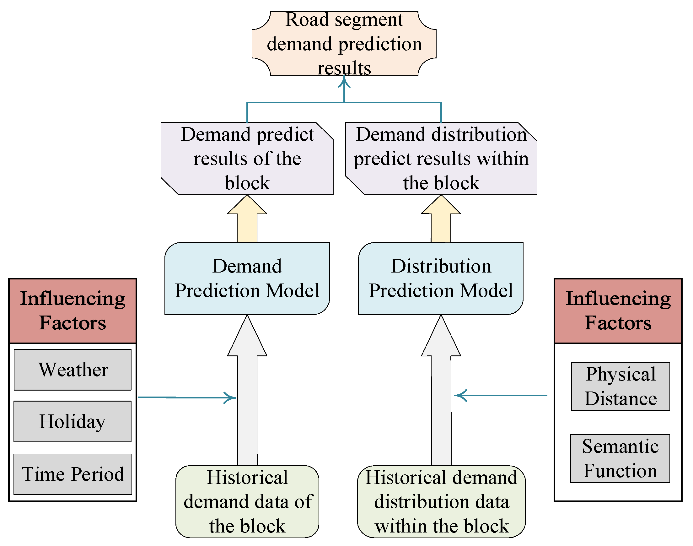
Figure 1. Structure of parking demand prediction model.
Sustainability 15 07096 g001
Figure 2. Impact of weather on parking demand of road sections (Workday). (a) Impact of weather on the parking demand of Lequn Road; (b) Impact of weather on the parking demand of Taiping Road.
Sustainability 15 07096 g002
Figure 3. Impact of holiday events on parking demand of road sections (Rainy). (a) Impact of holiday events on parking demand of Lequn Road; (b) Impact of holiday events on parking demand of Taiping Road.
Sustainability 15 07096 g003
Figure 4. Changes in parking demand at different times. (a) The different parking demand on Lequn Road at different times; (b) The different parking demand on Taiping Road at different times.
Sustainability 15 07096 g004
Figure 5. The structure of overall parking demand prediction.
Sustainability 15 07096 g005
Figure 6. Location of the road sections and examples of correlation between physical adjacency sections. (a) Location of each road section on the map; (b) Correlation between Lequn Road and Taiping Road; (c) Correlation between Sihui Road and Taiping Road; (d) Correlation between Sanhuang Road and Taiping Road.
Sustainability 15 07096 g006aSustainability 15 07096 g006b
Figure 7. Example of correlation between semantically similar sections. (a) Correlation between Lequn Road and Sanhuang Road; (b) Correlation between Sanhuang Road and Sihui Road.
Sustainability 15 07096 g007
Figure 8. The structure of internal demand distribution prediction.
Sustainability 15 07096 g008
Figure 9. Example of regional division.
Sustainability 15 07096 g009
Figure 10. Comparison of overall raw demand and prediction results (one week).
Sustainability 15 07096 g010
Figure 11. Comparison of original demand and forecast results for each road segment (one week). (a) Lequn Road; (b) Sanhuang Road; (c) Sihui Road; (d) Taiping Road.
Sustainability 15 07096 g011aSustainability 15 07096 g011b
Figure 12. Comparison of the predicted results of each model with ground truth (Lequn Road).
Sustainability 15 07096 g012
Figure 13. Comparison of one-day prediction results under the ablation experiment (Lequn Road).
Sustainability 15 07096 g013
Table 1. Results of the semantic functional similarity calculation between road segments.
Lequn RoadSanhuang RoadSihui RoadTaiping Road
Lequn Road10.844163430.899118930.95502897
Sanhuang Road0.8441634310.840448450.76167333
Sihui Road0.899118930.8404484510.78182478
Taiping Road0.955028970.761673330.781824781
Table 2. The number of parking spaces of the sections in the block shown in Figure 9.
RoadThe Number of Parking Spaces
Lequn Road42
Sanhuang Road18
Sihui Road26
Taiping Road29
Table 3. Comparison of demand prediction results of different models.
ModelRMSEMAE
HA4.0892.858
ARIMA3.8852.653
LSTM3.3542.568
GRU3.3472.556
GCN+GRU3.2482.505
HA+B&D3.8572.795
ARIMA+B&D3.5812.450
LSTM+B&D2.4941.917
GRU+B&D2.5011.915
GCN+GRU+B&D2.4371.882
ours2.2541.791
Table 4. Impact of different characteristics in demand prediction models.
ModelRMSEMAE
without weather2.3851.868
without external2.3801.872
without weather and external2.4291.874
without physical adjacency2.4181.898
without semantic function adjacency2.4411.913
ours2.2541.791
Disclaimer/Publisher’s Note: The statements, opinions and data contained in all publications are solely those of the individual author(s) and contributor(s) and not of MDPI and/or the editor(s). MDPI and/or the editor(s) disclaim responsibility for any injury to people or property resulting from any ideas, methods, instructions or products referred to in the content.