Article

On the Use of Reanalysis Data to Reconstruct Missing Observed Daily Temperatures in Europe over a Lengthy Period of Time

by
Konstantinos V. Varotsos
*,
George Katavoutas
and
Christos Giannakopoulos
Institute for Environmental Research and Sustainable Development, National Observatory of Athens, GR-15236 Athens, Greece
*
Author to whom correspondence should be addressed.
Sustainability 2023, 15(9), 7081; https://doi.org/10.3390/su15097081
Submission received: 24 February 2023 / Revised: 20 April 2023 / Accepted: 21 April 2023 / Published: 23 April 2023
(This article belongs to the Special Issue Climate Change and Urban Thermal Effects)

Abstract

:
In this study, a methodology that can reconstruct missing daily values of maximum and minimum temperatures over a long time period under the assumption of a sparse network of meteorological stations is described. To achieve this, a well-established software used for quality control, homogenization and the infilling of missing climatological series data, Climatol, is used to combine a mosaic of data, including daily observations from 15 European stations and daily data from two high-resolution reanalysis datasets, ERA5-Land and MESCAN-SURFEX; this is in order reconstruct daily values over the 2000–2018 period. By comparing frequently used indices, defined by the Expert Team on Climate Change Detection and Indices (ETCCDI) in studies of climate change assessment and goodness-of-fit measures, the reconstructed time series are evaluated against the observed ones. The analysis reveals that the ERA5-Land reconstructions outperform the MESCAN-SURFEX ones when compared to the observations in terms of biases, the various indices evaluated, and in terms of the goodness of fit for both the daily maximum and minimum temperatures. In addition, the magnitude and significance of the observed long-term temporal trends maintained in the reconstructions, in the majority of the stations examined, for both the daily maximum and daily minimum temperatures, is an issue of the greatest relevance in many climatic studies.

1. Introduction

Long-term near-surface observed temperature data are one of the essential climate variables that, as stated on the World’s Meteorological Organization webpage, “provide the empirical evidence needed to understand and predict the evolution of climate, to guide mitigation and adaptation measures, to assess risks and enable attribution of climate events to underlying causes, and to underpin climate services” [1]. In a practical context, long-term observational temperature records are useful in order to identify local trends in both the mean and extreme values of temperature (e.g., heatwaves, [2]) and to construct gridded observational datasets (e.g., [3,4,5] and references therein) that evaluate, bias adjust and statistically downscale temperature data from regional climate models and seasonal forecasts (e.g., [5,6,7,8,9,10]). Hence, long-term observational temperature data are of paramount importance in order to monitor the climate, detect trends, provide information about the occurrence of weather extremes, and improve and develop climate model projections that, in turn, can be used to provide climate change adaptation options for ecosystems (e.g., changes in structure and timing) and human systems (e.g., impacts on health and well-being, cities, settlements and infrastructure) [11,12,13,14].
Nevertheless, gaps in the time series due to instrument failures (fires, wars, earthquakes, floods) or due to technical limitation and/or limited resources compromise the quality and continuity of the meteorological records [15,16]. Data gaps prevent time series analyses from being statistically robust and can produce biased estimates, leading to invalid conclusions [17]. In addition, while new stations are installed, older ones are abandoned, making the inconsistencies between time series even higher. To overcome this drawback, various gap infilling procedures or methods used for the imputation of missing values are implemented prior to any statistical analysis of the data. In the general imputation of missing data, techniques may vary depending on the nature of the variables (i.e., categorical, numerical and mixed numerical and categorical). In the context of climatic studies (numerical variables), the methods range from using values from the same station (for instance, temperatures that exhibit high auto-correlation over time, temporal gap filling) or data from nearby stations (spatial gap filling). In the latter case, local gap filling is performed using observational data from neighboring station and deterministic (regression) methods, such as the K-nearest neighbors method, kriging, thin-plate splines and inverse distance weighting [18]. Meanwhile, recent studies have used bias adjustment methods, originally created for the bias correction of data output from climate models and to infill missing daily precipitation data [15,19]. In addition, more complex machine learning methods, such as support vector machines, the adaptive neuro-fuzzy inference system and decision trees, have also been used to infill missing temperature data [20]. While significant attempts have been made to reduce the error of gap-filling techniques, other important factors, such as maintaining the variability of the data or the magnitude and significance of the temporal trends, have received little attention. As a result, the reconstructed series are typically deflated, meaning that they exhibit less variability in relation to the true climate, while biases are found in the long term trends [18].
In areas with a sparse network of meteorological stations, nearby stations data can be replaced with data from gridded observational or reanalysis datasets. For instance, Way and Bonnaventure [21] combined temperature anomalies from gridded observational and reanalysis data sets with baseline climatologies from short observational records in order to infill monthly climate data in Canada for the period 2000–2009. In a similar way, Tang et al. [22] used various reanalysis datasets to produce station-based complete daily datasets of precipitation and temperature over North America (SCDNA) for the period 1979–2018; they utilized various techniques, such as quantile mapping, spatial interpolation and machine learning. However, in both cases (using data from nearby stations or the nearest grid points from reanalysis), issues arose during the gap-filling procedure over long time periods. In particular, Beguería et al. [18] found that reconstructed monthly temperature time series from nearby stations over several decades in Spain exhibited biases in the mean and variance, as well as departures from the observed long-term trends and their significance. Moreover, Tang et al. [22] found that although the SCDNA agrees well with station observations, better than the reanalysis datasets used in its production, the produced data series may not be appropriate for examining long-term trends in climate change studies since long-term trends are difficult to reconstruct in periods with missing data.
In this study, we present a trend-preserving methodology for reconstructing daily maximum and daily minimum air temperatures in Europe, assuming that there is a sparse network of meteorological stations using observational daily data and daily data from two gridded reanalysis datasets of high horizontal resolution. To our knowledge, this is the first study in which the reconstructed time series preserve the mean and the variability of the observed data while exhibiting similar levels of magnitude and significance to the observed long-term temporal trends, which is an issue of the greatest relevance in many climatic studies. The remainder of this paper is organized as follows. In Section 2, the datasets used in this study, as well as the methodology followed to reconstruct the missing values and the evaluation of the reconstructed time series against the missing observations, are presented. Section 3 presents and discusses the results, and Section 4 concludes the present study and the directions for future work are outlined.

2. Materials and Methods

2.1. Observed and Reanalysis Daily Datasets

In the present work, we used the available daily maximum (TX) and daily minimum (TN) air temperatures from 15 stations located within Europe (Table 1) for the period of 1981–2018. The observational data for all the stations except Athens and Nicosia were obtained from the European Climate Assessment Dataset (ECA&D, [23,24]), while the data for Athens were obtained from the historical meteorological station of the National Observatory of Athens (NOA, [25]) and the data for Nicosia were obtained from the Department of Meteorology in Cyprus [26]. The selection of these stations was based on the following criteria: (i) as wider European coverage as possible and (ii) an insignificant amount of missing data during the period of 1981–2018. Regarding the latter, in 9 out of the 15 stations, no missing data were found, while for the rest of the stations, the percentage of missing daily data was lower than 1%.
Moreover, for each station location, we extracted daily data for a number of surrounding grid points using a 1 degree radius from two reanalysis datasets, namely ERA5-Land [27] and MESCAN-SURFEX [28] for the period of 1981–2018. ERA5-Land is the high-resolution, approximately 9 km, land component of the ERA5 climate reanalysis dataset and provides hourly data for a number of variables from 1950 up to 2–3 months before the present day. MESCAN-SURFEX is a complementary surface analysis system to the UERRA-HARMONIE assimilation system that provides, among other essential climate variables, the air temperature recorded every six hours at 2 m above the model topography at a resolution of 5.5 km and for the period 1961–2019. The daily values for TX and TN were calculated using the hourly dataset of ERA5-Land and the 6-hourly dataset of SURFEX-MESCAN, with both datasets being available on the Copernicus Climate Data Store (CDS).

2.2. Daily Data Reconstruction

In this study, we aimed to reconstruct daily time series over a lengthy period of time. In order to achieve this, we considered that the available period of observational data for both the TX and TN covered the period 1981–1999, while we reconstructed the daily TX and TN for the period 2000–2018 in each station location (Figure 1).
For reconstructing the daily values over the period 2000–2018, the Climatol R-package was used [29]. Climatol is a well-established software used for quality control, homogenization and infilling the missing data of climatological series. For example, Coll et al. [30], after assessing the capabilities of four homogenization methods, namely Homer, Acmant, Climatol, and Ahops, to homogenize 299 of the available precipitation records for the island of Ireland, concluded that Climatol break detection findings should be used when the goals of the homogenization include the examination of station histories. In addition, Curci et al. [31] used Climatol to produce a long-term homogeneous climate dataset using monthly and daily observations of temperature and precipitation in the Abruzzo region in Central Italy.
The basis of Climatol’s operation is the calculation of sudden shifts (breaks) in anomalies at one station relative to time series at the same place calculated from data gathered at nearby stations [29]. In this study, the 10 land grid points closest to the stations’ locations, as obtained using both the ERA5-Land and MESCAN-SURFEX, were considered as nearby stations. To infill the missing data from the nearby reanalysis grid points, the reduced major axis regression was used [32]. Once the missing values were approximated, the Standard Normal Homogeneity Test (SNHT; [33]) was then used to test the homogeneity of the series using the series of anomalies that remain after data imputation. This was performed in order to (1) identify potential outliers and (2) test the series’ homogeneity. The series was divided in two at the moment the maximum SNHT was identified and whenever a series’ SNHT value exceeded the threshold (we used the default proposed value 25, but the user may alter it). The process was continued iteratively until no more inhomogeneous series were discovered. Additionally, because the SNHT test was unable to identify series with two or more breaks, the actual algorithm was applied in two stages: firstly, it was applied to series that were consistently divided into overlapping time windows, and secondly, it was applied to the entire series. The last stage was the reconstruction of the missing data, which can be applied to both monthly and daily time series. It should be noted that while the missing data reconstruction was carried out using the weighted mean of the closest four land grid points for the final stage (with weights given as a function of the distance), the first two stages used the unweighted mean data from the 10 nearest land grid points. In this study, we first applied Climatol to the mean monthly values and consequently, the break points that were identified were used for the reconstruction of the daily values. Additionally, we reconstructed the daily values for each year separately and in order, starting with the missing daily values for the year 2000 before applying the reconstruction to the following years, up until 2018.

2.3. Evaluation of the Reconstructed Daily Data

For each station in the dataset, we compared the reconstructed data with the observations for the period 1981–2018, as well as those for the reconstructed period, 2000–2018. To achieve this, apart from calculating the annual means and their temporal linear trends, a selection of indices from the Expert Team on Climate Change Detection and Indices (ETCCDI) [34] were examined (Table 2). In particular, for TX, these included the monthly maximum and minimum values for the daily maximum temperature (hereafter TXx and TXn, respectively), as well as the number of days with a daily TX higher than 25 °C and 35 °C (SU and SU35, respectively). In a similar way for TN, the monthly maximum and minimum values for the daily minimum temperature were calculated (hereafter TNx and TNn, respectively), as well as the number of days with a daily TN higher than 20 °C and 26 °C (TR and TR26, respectively). For the magnitude of the linear temporal trends over the examined periods, the Sein–Theil estimator was used [35,36], while the statistical significance of the results was assessed using the 95th percentile confidence intervals, as derived by the bootstrap method [5,9,37,38,39]. In addition, for the reconstruction period 2000–2018, and for the daily scale, the Kling–Gupta efficiency (KGE) between the reconstructed and observed values was used [40]. KGE is a goodness-of-fit measure that has values ranging between −Inf and 1. In our case, the reconstruction was more accurate if the KGE values were closer to 1. Three key factors were taken into account when calculating the KGE: (i) the Pearson product–moment correlation coefficient (R); (ii) the proportion of the mean of the reconstructed values to the mean of the observed values (Beta); and (iii) the variability ratio, using the standard deviations of the reconstructed values to the observed ones (Alpha).

3. Results and Discussion

3.1. TX Reconstructions

In Figure 2, the comparison between the observational data and the reconstructed datasets using both ERA5-Land and MESCAN-SURFEX for the average annual TX and selected indices, for all stations and for the period 1981–2018, is shown. It is noted that the period of 1981–1999 is common in all three time series, while the reconstructed period covers the period of 2000–2018. From the figure, it is evident that the absolute mean differences between the observed and the reconstructed time series in terms of the average annual TX are lower than approximately 0.2 °C and 0.4 °C for the reconstructions based on ERA5-Land and MESCAN-SURFEX, respectively, with the differences found statistically significant only for the reconstructions of Nicosia and Athens using the latter reanalysis dataset.
Regarding the linear trends observed in the average annual TX, the results indicate similar positive slopes to those observed for the ERA5-Land reconstructions, with deviations being lower than approximately 0.1 °C/decade; meanwhile, for the MESCAN-SURFEX reconstructions, the highest overestimations of the observed trends were found in Nicosia, Athens and Rotterdam, reaching approximately 0.4 °C/decade in the first two stations and approximately 0.3 °C/decade in the latter station, respectively. As far as the average TXx and TXn are concerned for both indices, the reconstructed time series indicate similar results to those observed. The absolute deviations for TXx were found to be lower than 0.7 °C and 1.6 °C for the reconstructions based on ERA5-Land and MESCAN-SURFEX, respectively, while for TXn, these were found to be lower than 0.3 °C and 1.1 °C for both reconstructions, respectively. Results similar to those observed for the TX threshold-based indices, SU and SU35, were found for both reconstructed datasets.
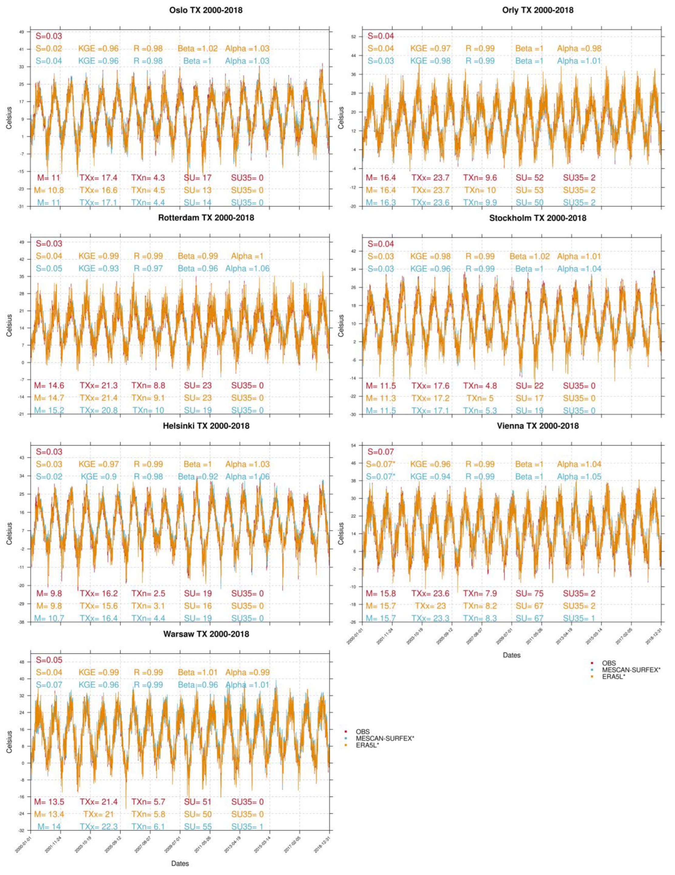
Figure 3 illustrates the daily observational data and their daily reconstructions using ERA5-Land and MESCAN-SURFEX in each one of the stations over the period 2000–2018. In general, it is evident that the ERA5-Land reconstructions perform better than the MESCAN-SURFEX ones when compared to the observations, with the average KGE over all stations being 0.97 (KGE range 0.92–0.99) and 0.94 (KGE range 0.86–0.98) for the two reconstructions, respectively. Moreover, from examining the results at each station, it is evident that for the reconstructed KGE values > 0.95, the magnitude of the slopes and the mean values of the average annual TX, as well as the averaged values of the rest of the indices examined, indicate the lowest level of deviation from the observed ones.

3.2. TN Reconstructions

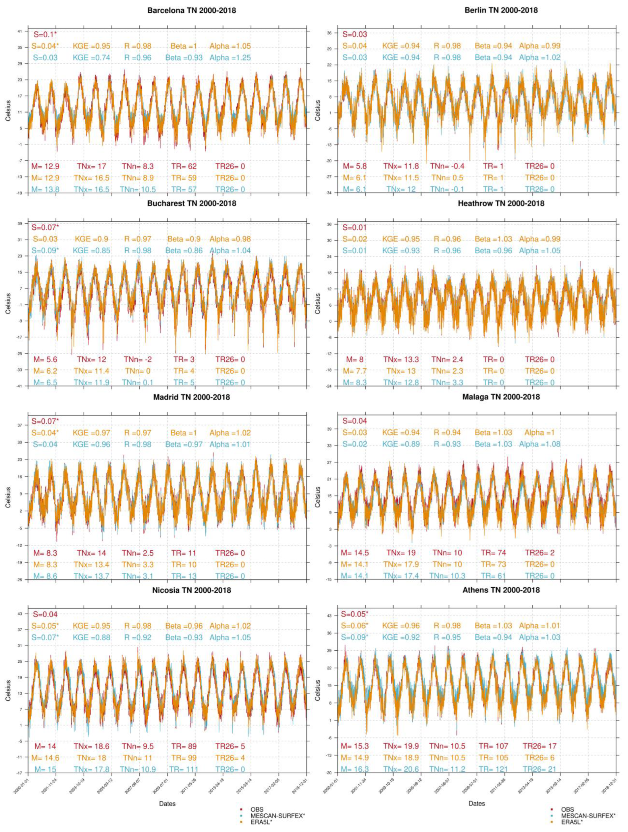
Similar results to the TX reconstructions for the period 1981–2018 were found for TN (Figure 4). For the reconstructions based on ERA5-Land and MESCAN-SURFEX, respectively, the absolute mean differences between the observed and reconstructed time series in the average annual TN were less than approximately 0.3 °C and 0.7 °C, with the differences found to be statistically significant only for the reconstructions of Bucharest, Nicosia, and Vienna using the MESCAN-SURFEX reanalysis dataset. In terms of the linear trends observed in the average annual TN, ERA5-Land reconstructions indicate similar positive slopes to those observed, with the deviations being lower than approximately 0.2 °C/decade; meanwhile, for the MESCAN-SURFEX ones, the highest overestimations of the observed trends were found in Bucharest, Nicosia, Athens and Vienna, reaching approximately 0.4 °C/decade in the first three stations and approximately 0.5 °C/decade in the latter station. As far as the average TNx and TNn are concerned, for both indices the reconstructed time series indicate similar results to those observed. The absolute deviations for TNx were found to be lower than approximately 0.7 °C and 0.8 °C for the reconstructions based on ERA5-Land and MESCAN-SURFEX, respectively, while for TXn, these were found to be lower than approximately 1.0 °C and 1.4 °C for both reconstructions, respectively. Results similar to the observed results were found for the TN threshold-based indices, TR and TR26, for both the reconstructed datasets and for the majority of the stations.
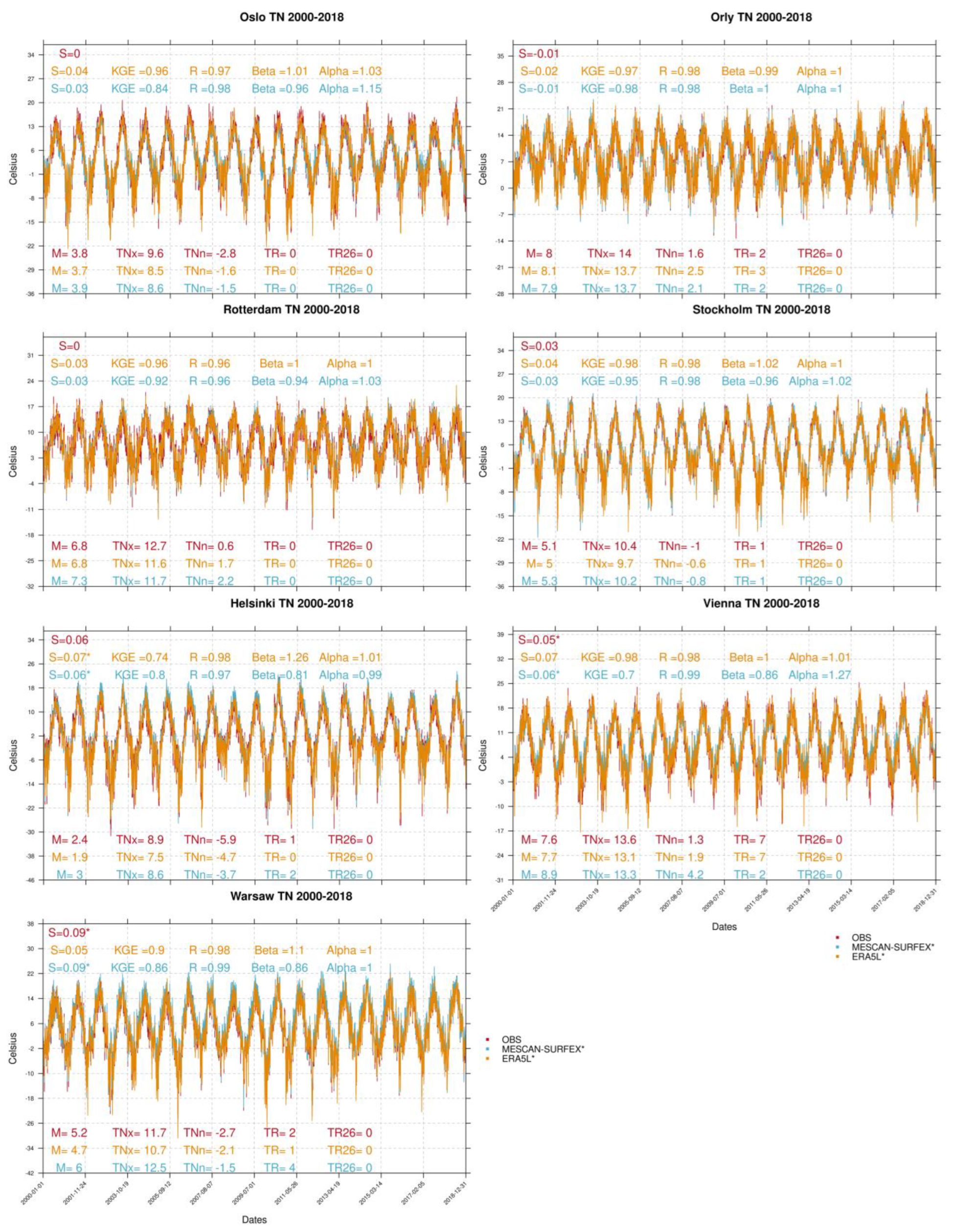
As far as the daily values during the reconstruction period are concerned (Figure 5), the results indicate lower average KGE values compared to the TX ones among all stations; these were 0.94 (KGE range 0.74–0.98) and 0.88 (KGE range 0.70–0.98) for the ERA5-Land and MESCAN-SURFEX reconstructions, respectively. However, in the majority of the stations, the linear trends observed in the average annual TN were maintained, while the correlation coefficients on the daily scale between the observed and the reconstructed time series were higher than 0.92 in all stations.

3.3. Discussion

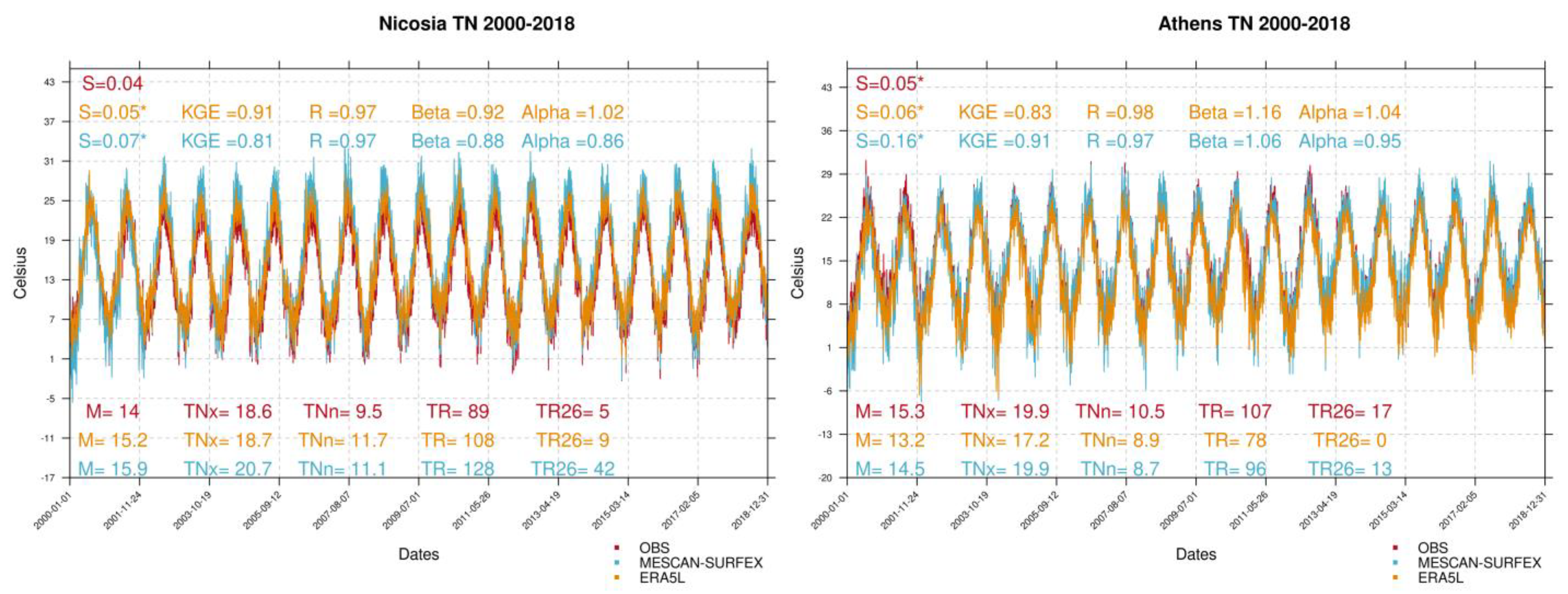
The results presented in the previous section indicate that both reanalysis datasets can be used in the reconstruction of the daily maximum and minimum temperatures, with the ERA5-Land reconstructions performing better than the MESCAN-SURFEX ones when compared to the observations; meanwhile, both the reconstructions indicated a better overall statistical performance when compared to the raw reanalysis output. This can be seen by contrasting the results in Figure 6, which compare the observations and raw data from the closest grid point from ERA5-Land and MESCAN-SURFEX for two stations, Nicosia and Athens, and throughout the period 2000–2018 for TN, with the corresponding results in Figure 5. The better performance of the ERA5-Land reconstructions is mostly driven by the better performance of the raw ERA5-Land dataset. In particular, a recent study comparing both ERA5-Land and MESCAN-SURFEX against local spatially interpolated weather station data in the Campania Region of Italy found that for a number of meteorological variables, ERA5-Land outperformed MESCAN-SURFEX [41]. This behavior was attributed to the fact that ERA5-Land incorporates lapse rate corrections to account for the influence of elevation on meteorological variables when downscaled from the ERA5 global reanalysis; meanwhile, MESCAN-SURFEX, although having a higher resolution, is highly influenced by the previous generation ERA-Interim global reanalysis, which was used to drive the UERRA-HARMONIE regional reanalysis.
Regarding the length of the reconstructions in Section 3, the results include the daily reconstruction of the data of 19 years that has 50% non-missing data (19 years) over the 1981–2018 period. Tests with ERA5-Land indicate that the reconstruction methodology performs reasonably well for a higher number of reconstructed years, i.e., reconstructing daily values in the period 1991–2018. In addition, the method can be used for reconstructing the daily time series backwards in time.
The methodology presented in this study may be useful in areas with a sparse network of meteorological stations and/or in areas with a complex topography. In addition, gridded observational datasets may benefit from the lengthy period reconstructions proposed in this study. For instance, in E-OBS (current version v26.0e, [3]), the majority of the stations from Greece included in the daily TX and TN interpolation procedure provide data until 2004. The infilling of missing data methodology presented in this study could be used to reconstruct the missing years, prior to the interpolation procedure implemented in E-OBS, in order to expand the gridded datasets’ time coverage up to 2–3 months before the present if, for instance, using ERA5-Land.

4. Conclusions

Assuming a sparse network of meteorological stations, an approach to reconstructing missing daily values of maximum and minimum temperatures over a lengthy time period was presented in this study. In order to accomplish this, a collection of data, including daily observations from 15 European stations and daily data from two high-resolution reanalysis datasets, ERA5-Land and MESCAN-SURFEX, was combined using the Climatol software. The reconstructed time series were evaluated against the observed ones by comparing indices, as specified by the Expert Team on Climate Change Detection and Indices (ETCCDI), frequently used in studies of climate change assessment as well as goodness-of-fit metrics. When compared to the observations, the analysis showed that the ERA5-Land reconstructions performed better than the MESCAN-SURFEX ones in terms of biases, among the many indices considered, and in terms of the goodness of fit for both the daily maximum and minimum temperatures. Moreover, the extent and significance of the observed long-term temporal trends were also preserved in the reconstructions for both the daily maximum and daily minimum temperatures; this is a topic of particular importance in many climatic studies and at the majority of the stations examined. The methods described in this paper may be helpful in areas with a sparse network of meteorological stations and/or in places with a complex topography. The lengthy period reconstructions obtained in this study may also be useful in the production of gridded observational datasets. Future work will focus on applying the reconstruction methodology to other variables such as precipitation, wind speed and relative humidity.

Author Contributions

Conceptualization, K.V.V.; methodology, K.V.V.; software, K.V.V.; validation, K.V.V. and G.K.; formal analysis, K.V.V.; investigation, K.V.V.; resources, C.G.; data curation, K.V.V. and G.K.; writing—original draft preparation, K.V.V.; writing—review and editing, K.V.V., G.K. and C.G.; funding acquisition, C.G. All authors have read and agreed to the published version of the manuscript.

Funding

This research has received funding from the European Union’s Horizon 2020 research and innovation program ‘Climate-resilient regions through systemic solutions and innovations, ARSINOE’ under grant agreement 101037424.

Institutional Review Board Statement

Not applicable.

Informed Consent Statement

Not applicable.

Data Availability Statement

The data analyzed in this study can be found at https://www.ecad.eu (accessed on 20 October 2022) for all stations except Athens and Nicosia, at https://data.climpact.gr/en/dataset (accessed on 20 October 2022) for Athens (NOA) and at http://www.moa.gov.cy/moa/dm/dm.nsf/home_en/home_en?openform (accessed on 20 October 2022) for Nicosia.

Acknowledgments

We acknowledge the data providers in the ECA&D project (data and metadata available at https://www.ecad.eu (accessed on 20 October 2022); [24]) and the CLIMPACT project (https://climpact.gr/main/, accessed on 20 October 2022), as well as the Department of Meteorology in Cyprus (http://www.moa.gov.cy/moa/dm/dm.nsf/home_en/home_en?openform, accessed on 20 October 2022).

Conflicts of Interest

The authors declare no conflict of interest.

References

  1. World Meteorological Organization. Available online: https://public.wmo.int/en/programmes/global-climate-observing-system/essential-climate-variables (accessed on 14 November 2022).
  2. Founda, D.; Katavoutas, G.; Pierros, F.; Mihalopoulos, N. Centennial changes in heat waves characteristics in Athens (Greece) from multiple definitions based on climatic and bioclimatic indices. Glob. Planet. Chang. 2022, 212, 103807. [Google Scholar] [CrossRef]
  3. Cornes, R.C.; van der Schrier, G.; van den Besselaar, E.J.M.; Jones, P.D. An ensemble version of the E-OBS temperature and precipitation data sets. J. Geophys. Res. Atmos. 2018, 123, 9391–9409. [Google Scholar] [CrossRef]
  4. Herrera, S.; Cardoso, R.M.; Soares, P.M.; Espírito-Santo, F.; Viterbo, P.; Gutiérrez, J.M. Iberia01: A new gridded dataset of daily precipitation and temperatures over Iberia. Earth Syst. Sci. Data 2019, 11, 1947–1956. [Google Scholar] [CrossRef]
  5. Varotsos, K.V.; Dandou, A.; Papangelis, G.; Roukounakis, N.; Kitsara, G.; Tombrou, M.; Giannakopoulos, C. Using a new local high resolution daily gridded dataset for Attica to statistically downscale climate projections. Clim. Dyn. 2022, 60, 2931–2956. [Google Scholar] [CrossRef]
  6. van der Schriek, T.; Varotsos, K.V.; Giannakopoulos, C.; Founda, D. Projected future temporal trends of two different urban heat islands in Athens (Greece) under three climate change scenarios: A statistical approach. Atmosphere 2020, 11, 637. [Google Scholar] [CrossRef]
  7. Manzanas, R.; Gutiérrez, J.M.; Bhend, J.; Hemri, S.; Doblas-Reyes, F.J.; Torralba, V.; Penabad, E.; Brookshaw, A. Bias adjustment and ensemble recalibration methods for seasonal forecasting: A comprehensive intercomparison using the C3S dataset. Clim. Dyn. 2019, 53, 1287–1305. [Google Scholar] [CrossRef]
  8. Gratsea, M.; Varotsos, K.V.; López-Nevado, J.; López-Feria, S.; Giannakopoulos, C. Assessing the long-term impact of climate change on olive crops and olive fly in Andalusia, Spain, through climate indices and return period analysis. Clim. Serv. 2022, 28, 100325. [Google Scholar] [CrossRef]
  9. Varotsos, K.V.; Karali, A.; Lemesios, G.; Kitsara, G.; Moriondo, M.; Dibari, C.; Leolini, L.; Giannakopoulos, C. Near future climate change projections with implications for the agricultural sector of three major Mediterranean islands. Reg. Environ. Chang. 2021, 21, 16. [Google Scholar] [CrossRef]
  10. Karali, A.; Varotsos, K.V.; Giannakopoulos, C.; Nastos, P.P.; Hatzaki, M. Seasonal fire danger forecasts for supporting fire prevention management in an eastern Mediterranean environment: The case study of Attica, Greece. Nat. Hazards Earth Syst. Sci. 2023, 23, 429–445. [Google Scholar] [CrossRef]
  11. IPCC. Summary for Policymakers. In Climate Change 2022: Impacts, Adaptation and Vulnerability. Contribution of Working Group II to the Sixth Assessment Report of the Intergovernmental Panel on Climate Change; Pörtner, H.-O., Roberts, D.C., Poloczanska, E.S., Mintenbeck, K., Tignor, M., Alegría, A., Craig, M., Langsdorf, S., Löschke, S., Möller, V., et al., Eds.; Cambridge University Press: Cambridge, UK; New York, NY, USA, 2022; pp. 3–33. [Google Scholar] [CrossRef]
  12. Abbas, A.; Waseem, M.; Ullah, W.; Zhao, C.; Zhu, J. Spatiotemporal analysis of meteorological and hydrological droughts and their propagations. Water 2021, 13, 2237. [Google Scholar] [CrossRef]
  13. Elahi, E.; Khalid, Z.; Tauni, M.Z.; Zhang, H.; Lirong, X. Extreme weather events risk to crop-production and the adaptation of innovative management strategies to mitigate the risk: A retrospective survey of rural Punjab, Pakistan. Technovation 2022, 117, 102255. [Google Scholar] [CrossRef]
  14. Nhemachena, C.; Nhamo, L.; Matchaya, G.; Nhemachena, C.R.; Muchara, B.; Karuaihe, S.T.; Mpandeli, S. Climate change impacts on water and agriculture sectors in Southern Africa: Threats and opportunities for sustainable development. Water 2020, 12, 2673. [Google Scholar] [CrossRef]
  15. Grillakis, M.G.; Polykretis, C.; Manoudakis, S.; Seiradakis, K.D.; Alexakis, D.D. A quantile mapping method to fill in discontinued daily precipitation time series. Water 2020, 12, 2304. [Google Scholar] [CrossRef]
  16. Costa, R.L.; Barros Gomes, H.; Cavalcante Pinto, D.D.; da Rocha Júnior, R.L.; dos Santos Silva, F.D.; Barros Gomes, H.; Lemos da Silva, M.C.; Luís Herdies, D. Gap Filling and Quality Control Applied to Meteorological Variables Measured in the Northeast Region of Brazil. Atmosphere 2021, 12, 1278. [Google Scholar] [CrossRef]
  17. Dinh, D.-T.; Huynh, V.-N.; Sriboonchitta, S. Clustering mixed numerical and categorical data with missing values. Inf. Sci. 2021, 571, 418–442. [Google Scholar] [CrossRef]
  18. Beguería, S.; Tomas-Burguera, M.; Serrano-Notivoli, R.; Peña-Angulo, D.; Vicente-Serrano, S.M.; González-Hidalgo, J.C. Gap filling of monthly temperature data and its effect on climatic variability and trends. J. Clim. 2019, 32, 7797–7821. [Google Scholar] [CrossRef]
  19. Devi, U.; Shekhar, M.S.; Singh, G.P.; Rao, N.N.; Bhatt, U.S. Methodological application of quantile mapping to generate precipitation data over Northwest Himalaya. Int. J. Climatol. 2019, 39, 3160–3170. [Google Scholar] [CrossRef]
  20. Katipoğlu, O.M. Prediction of missing temperature data using different machine learning methods. Arab. J. Geosci. 2022, 15, 21. [Google Scholar] [CrossRef]
  21. Way, R.G.; Bonnaventure, P.P. Testing a reanalysis-based infilling method for areas with sparse discontinuous air temperature data in northeastern Canada. Atmos. Sci. Lett. 2015, 16, 398–407. [Google Scholar] [CrossRef]
  22. Tang, G.; Clark, M.P.; Newman, A.J.; Wood, A.W.; Papalexiou, S.M.; Vionnet, V.; Whitfield, P.H. SCDNA: A serially complete precipitation and temperature dataset for North America from 1979 to 2018. Earth Syst. Sci. Data 2020, 12, 2381–2409. [Google Scholar] [CrossRef]
  23. European Climate Assessment & Dataset. Available online: https://www.ecad.eu/dailydata/index.php (accessed on 3 October 2022).
  24. Klein Tank, A.M.G.; Wijngaard, J.B.; Können, G.P.; Böhm, R.; Demarée, G.; Gocheva, A.; Mileta, M.; Pashiardis, S.; Hejkrlik, L.; Kern-Hansen, C.; et al. Daily dataset of 20th-century surface air temperature and precipitation series for the European Climate Assessment. Int. J. Climatol. 2002, 22, 1441–1453. [Google Scholar] [CrossRef]
  25. CLIMPACT–National Network for Climate Change and Its Impact. Available online: https://data.climpact.gr/en/dataset (accessed on 5 October 2022).
  26. Department of Meteorology, Republic of Cyprus. Available online: http://www.moa.gov.cy/moa/dm/dm.nsf/home_en/home_en?openform (accessed on 7 October 2022).
  27. Muñoz-Sabater, J.; Dutra, E.; Agustí-Panareda, A.; Albergel, C.; Arduini, G.; Balsamo, G.; Boussetta, S.; Choulga, M.; Harrigan, S.; Hersbach, H.; et al. ERA5-Land: A state-of-the-art global reanalysis dataset for land applications. Earth Syst. Sci. Data 2021, 13, 4349–4383. [Google Scholar] [CrossRef]
  28. Bazile, E.; Abida, R.; Verelle, A.; Le Moigne, P.; Szczypta, C. MESCAN-SURFEX Surface Analysis. Deliverable D2.8 of the UERRA Project 2017. Available online: http://www.uerra.eu/publications/deliverable-reports.html (accessed on 14 October 2022).
  29. Guijarro, J.A. Package ‘Climatol’. Available online: https://cran.r-project.org/web/packages/climatol/climatol.pdf (accessed on 20 April 2020).
  30. Coll, J.; Domonkos, P.; Guijarro, J.; Curley, M.; Rustemeier, E.; Aguilar, E.; Walsh, S.; Sweeney, J. Application of homogenization methods for Ireland’s monthly precipitation records: Comparison of break detection results. Int. J. Climatol. 2020, 40, 6169–6188. [Google Scholar] [CrossRef] [PubMed]
  31. Curci, G.; Guijarro, J.A.; Di Antonio, L.; Di Bacco, M.; Di Lena, B.; Scorzini, A.R. Building a local climate reference dataset: Application to the Abruzzo region (Central Italy), 1930–2019. Int. J. Climatol. 2021, 41, 4414–4436. [Google Scholar] [CrossRef]
  32. Harper, W.V. Reduced major axis regression. In Wiley StatsRef: Statistics Reference Online; John Wiley & Sons, Inc.: Hoboken, NJ, USA, 2016. [Google Scholar] [CrossRef]
  33. Alexandersson, H. A homogeneity test applied to precipitation data. J. Clim. 1986, 6, 661–675. [Google Scholar] [CrossRef]
  34. Zhang, X.; Alexander, L.; Hegerl, G.C.; Jones, P.; Tank, A.K.; Peterson, T.C.; Trewin, B.; Zwiers, F.W. Indices for monitoring changes in extremes based on daily temperature and precipitation data. Wiley Interdiscip. Rev. Clim. Chang. 2011, 2, 851–870. [Google Scholar] [CrossRef]
  35. Theil, H. A rank-invariant method of linear and polynomial regression analysis. Indag. Math. 1950, 12, 173. [Google Scholar]
  36. Sen, P.K. Estimates of the regression coefficient based on Kendall’s tau. J. Am. Stat. Assoc. 1968, 63, 1379–1389. [Google Scholar] [CrossRef]
  37. Efron, B. Better bootstrap confidence intervals. J. Am. Stat. Assoc. 1987, 82, 171–185. [Google Scholar] [CrossRef]
  38. Wilcox, R.R. Introduction to Robust Estimation and Hypothesis Testing, 1st ed.; Academic Press: Waltham, MA, USA, 2012; pp. 1–690. [Google Scholar]
  39. Varotsos, K.V.; Giannakopoulos, C.; Tombrou, M. Ozone-temperature relationship during the 2003 and 2014 heatwaves in Europe. Reg. Environ. Chang. 2019, 19, 1653–1665. [Google Scholar] [CrossRef]
  40. Gupta, H.V.; Kling, H.; Yilmaz, K.K.; Martinez, G.F. Decomposition of the mean squared error and NSE performance criteria: Implications for improving hydrological modelling. J. Hydrol. 2009, 377, 80–91. [Google Scholar] [CrossRef]
  41. Pelosi, A.; Terribile, F.; D’Urso, G.; Chirico, G.B. Comparison of ERA5-Land and UERRA MESCAN-SURFEX reanalysis data with spatially interpolated weather observations for the regional assessment of reference evapotranspiration. Water 2020, 12, 1669. [Google Scholar] [CrossRef]
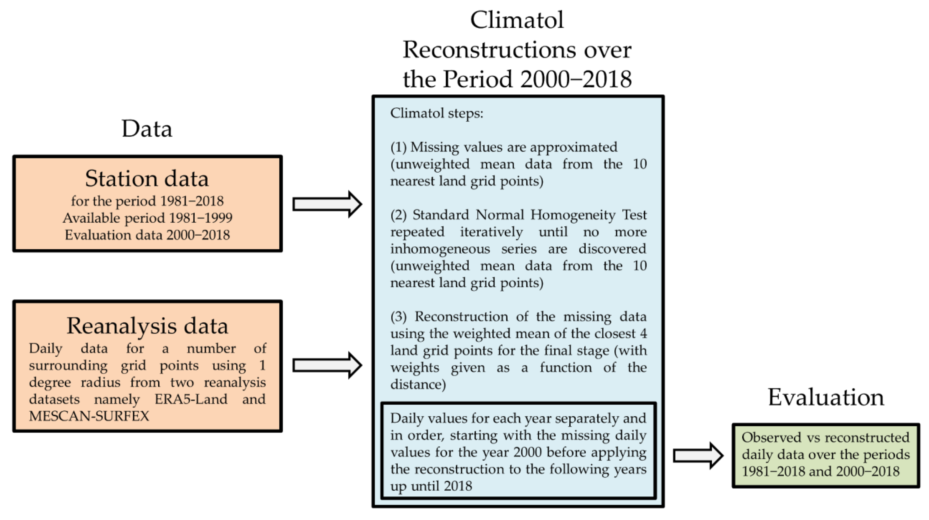
Figure 1. Flowchart illustrating the methodology used to reconstruct the daily maximum and minimum temperatures over the period 2000–2018 and the evaluation analysis followed.
Sustainability 15 07081 g001
Figure 2. Average annual maximum temperatures over the period of 1981–2018 for the observations (OBS, with red color), as well as the reconstructions obtained using ERA5-Land (ERA5L*, with orange color) and MESCAN-SURFEX (MESCAN-SURFEX*, with blue color) for all station locations. In each panel, M indicates the average annual value of TX (in °C/year); S is the annual trend, as derived using Sen’s method, with an asterisk indicating a statistically significant trend (°C/year); TXx and TXn are the average maximum and minimum monthly temperatures, respectively (°C/year); and SU and SU35 are the average annual number of days with a daily TX higher than 25 °C and 35 °C, respectively.
Sustainability 15 07081 g002
Figure 3. Daily maximum temperatures over the period 2000–2018 for the observations (OBS, with red color), as well as the reconstructions obtained from ERA5-Land (ERA5L*, with orange color) and MESCAN-SURFEX (MESCAN-SURFEX*, with blue color) for all station locations. In each panel, M indicates the average annual value of TX (in °C/year); S is the annual trend, as derived using Sen’s method, with an asterisk indicating a statistically significant trend (°C/year); TXx and TXn are the average maximum and minimum monthly temperatures, respectively (°C/year); and SU and SU35 are the average annual number of days with a daily TX higher than 25 °C and 35 °C, respectively. KGE indicates the value of the Kling–Gupta efficiency measure between the observed daily values and the reconstructed ones, and the factors used for KGE calculations: the Pearson product–moment correlation coefficient (R); the proportion of the mean of the reconstructed values to the mean of the observed values (Beta); and the variability ratio, using the standard deviations of the reconstructed values to the observed ones (Alpha).
Sustainability 15 07081 g003aSustainability 15 07081 g003b
Figure 4. Average annual minimum temperatures over the period 1981–2018 for the observations (OBS, with red color), as well as the reconstructions obtained from ERA5-Land (ERA5L*, with orange color) and MESCAN-SURFEX (MESCAN-SURFEX*, with blue color) for all station locations. In each panel, M indicates the average annual value of TN (in °C/year); S is the annual trend, as derived using Sen’s method, with an asterisk indicating a statistically significant trend (°C/year); TNx and TNn are the average maximum and minimum monthly temperatures, respectively (°C/year); and TR and TR26 are the average annual number of days with a daily TN higher than 20 °C and 26 °C, respectively.
Sustainability 15 07081 g004
Figure 5. Daily minimum temperatures over the period 2000–2018 for the observations (OBS, with red color), as well as the reconstructions obtained from ERA5-Land (ERA5L*, with orange color) and MESCAN-SURFEX (MESCAN-SURFEX*, with blue color) for all station locations. In each panel, M indicates the average annual value of TN (in °C/year); S is the annual trend, as derived using Sen’s method, with an asterisk indicating a statistically significant trend (°C/year); TNx and TNn are the average maximum and minimum monthly temperatures, respectively (°C/year); and TR and TR26 are the average annual number of days with a daily TN higher than 20 °C and 26 °C, respectively. KGE indicates the value of the Kling–Gupta efficiency measure between the observed daily values and the reconstructed ones, and the factors used for KGE calculations: the Pearson product–moment correlation coefficient (R); the proportion of the mean of the reconstructed values to the mean of the observed values (Beta); and the variability ratio, using the standard deviations of the reconstructed values to the observed ones (Alpha).
Sustainability 15 07081 g005aSustainability 15 07081 g005b
Figure 6. Daily minimum temperatures over the period 2000–2018 for the observations (OBS, with red color), as well as the data obtained from the closet grid point to the station locations from ERA5-Land (ERA5L, with orange color) and MESCAN-SURFEX (with blue color) for two stations. In each panel, M indicates the average annual value of TN (in °C/year); S is the annual trend, as derived using Sen’s method, with an asterisk indicating a statistically significant trend (°C/year); TNx and TNn are the average maximum and minimum monthly temperatures, respectively (°C/year); and TR and TR26 are the average annual number of days with a daily TN higher than 20 °C and 26 °C, respectively. KGE indicates the value of the Kling–Gupta efficiency measure between the observed daily values and the reconstructed ones, and the factors used for KGE calculations: the Pearson product–moment correlation coefficient ®, the proportion of the mean of the reconstructed values to the mean of the observed values (Beta); and the variability ratio, using the standard deviations of the reconstructed values to the observed ones (Alpha).
Sustainability 15 07081 g006
Table 1. List of the weather stations used.
Station NameECA&D Station IDLongitudeLatitudeElevation (m.a.s.l)
Barcelona29692.0741.294
Berlin4113.3052.4651
Bucharest21926.0844.5290
Heathrow1860−0.4551.4825
Madrid3946−3.5640.47609
Malaga231−4.4936.677
Nicosia-33.4035.14160
Athens-23.7237.97107
Oslo19310.7259.9494
Orly11,2492.3848.7289
Rotterdam5984.4551.96−4
Stockholm1018.0559.3544
Helsinki699224.9660.3351
Vienna1616.3648.25198
Warsaw20920.9652.16107
Table 2. List of ETCCDI indices examined and statistical measures used in the evaluation analysis.
DescriptionAbbreviations
Daily maximum air temperatureTX
Daily minimum air temperatureTN
Monthly maximum value of daily maximum temperatureTXx
Monthly minimum value of daily maximum temperatureTXn
Number of days with daily TX higher than 25 °CSU
Number of days with daily TX higher than 35 °CSU35
Monthly maximum value of daily minimum temperatureTNx
Monthly minimum value of daily minimum temperatureTNn
Number of days with daily TN higher than 20 °CTR
Number of days with daily TN higher than 26 °CTR26
Kling-Gupta efficiencyKGE
Pearson product–moment correlation coefficientR
Proportion of the mean of the reconstructed values to the mean of the observed valuesBeta
Variability ratio, using the standard deviations of the reconstructed values to the observed onesAlpha
Annual trend, as derived by Sen’s method (asterisk indicates statistically significant trend)S
Disclaimer/Publisher’s Note: The statements, opinions and data contained in all publications are solely those of the individual author(s) and contributor(s) and not of MDPI and/or the editor(s). MDPI and/or the editor(s) disclaim responsibility for any injury to people or property resulting from any ideas, methods, instructions or products referred to in the content.