The Effect of Power Flow Entropy on Available Load Supply Capacity under Stochastic Scenarios with Different Control Coefficients of UPFC

Abstract

With the sharp increase in fluctuant sources in power systems, the deterministic power flow (DPF) calculation has been unable to meet the demands of practical applications; thus, the probabilistic method becomes indispensable for the reliable and stable operation of power systems. This paper adopts the probabilistic power flow (PPF) method, which is a Monte Carlo simulation (MCS) based on the Latin hypercube sampling (LHS) method, to analyze the uncertainties of power systems. Specifically, the available load supply capability (ALSC) based on the branch loading rate is used to analyze the safety margin of the whole system, while the improved power flow entropy is introduced to quantify the equilibrium of power flow distribution. The repeated power flow (RPF) calculation is combined with the PPF method, and, hence, the probabilistic repeated power flow (PRPF) method is proposed to calculate the power flow entropy at the initial state and the probabilistic ALSC. To flexibly control the power flow, the unified power flow controller (UPFC) is added to the AC power system. The different control coefficients of UPFC are set to reveal the relationship between power flow entropy and available load supply capability under the stochastic scenarios. Finally, the modified IEEE14 test system is used to study the adjustment abilities of UPFC. With consideration of uncertainties in the test case, the positive effect of UPFC on the power flow entropy and the probabilistic ALSC under stochastic scenarios is deeply studied.

1. Introduction

With the continuous expansion of the AC power grids, the uncertainties of the load increase and large-scale integration of renewable energies have increased the randomness of the power system [1]. Renewable energies have the advantages of cleanness and sustainability, which can break out of human dependence on fossil energy. It is necessary to study the impact of these renewable energies on the power system, which can further make the development of power systems more sustainable. However, the deterministic power flow (DPF) calculation is not applicable when analyzing the AC system with renewable energies. The probabilistic power flow (PPF) could be introduced to analyze these situations [2]. PPF can fully consider the influence of random inputs of the system, aiming at obtaining the mean value, variance, and probabilistic distribution of target outputs, such as the bus voltage and branch power. PPF calculation is mainly divided into three methods: the Monte Carlo simulation (MCS) method, the approximation method, and the analytical method [3,4]. The basic idea of the MCS can be briefly described as follows: to perform probabilistic analysis, a probabilistic model or stochastic process is first constructed; through a batch of samplings, we obtain the frequency of the events to estimate the probability of occurrence [5]. The most traditional MCS method is based on random sampling (RS-MCS). This method is computationally time-consuming and inefficient. However, the RS-MCS method can also have high accuracy if the input samples are sufficiently large, without being limited to the dimension and distribution of the input. Therefore, the RS-MCS method is often used as a reference for other methods. The Latin hypercube sampling (LHS) is a typical stratified sampling method that can effectively improve sampling efficiency [6]. The MCS method based on the LHS method (LHS-MCS), in combination with DPF, is an effective PPF method to improve the computational efficiency, and it has been widely used [7,8]. At the same time, there are further challenges to the reliable power supply due to uncertainties in the grid. A metric and operation strategy should be sought to improve the system availability for safer operation. The supply capacity of the system load can be used as an indicator of system reliability [9]. To reveal the characteristics of the system operation, the available load supply capability (ALSC) is introduced [10]. ALSC shows the ability to increase the load until any system constraint is not satisfied. Obviously, the larger the percentage that the load can grow, the better the redundancy of the system is. Therefore, to face some extreme scenarios, the system should have higher available power for a more reliable operation. To evaluate ALSC, many indicators are available, such as voltage eligibility rate, voltage stability, N–1 principle, branch loading rate, and so forth [11,12]. In the operation of the power grid, the capacity of the branch often limits the amount of the power transmitted from the power supply side to the load side. Therefore, the branch loading rate is a good index to measure the ALSC. Furthermore, the repeated power flow (RPF) calculation is an appropriate method for determining ALSC [13,14]. However, most of the current research focuses on the analysis of ALSC, but without adopting a positive approach to adjust it [10,11,12].

The branch loading rate can quantify the transmission power of each branch, so it is necessary to analyze the reasonable distribution of the system power flow. The disordered load distribution, improper power network architecture, and the uncoordinated parameters may cause an uneven power flow distribution [15]. The unexpected distribution of power flow is not only detrimental to the redundancy and economic operation of the system, but also poses a risk to the reliable power supplement [16]. Therefore, it is also necessary to seek an index that describes the equilibrium degree of power flow distribution in the system. The power flow entropy, which highly depends on the branch loading rate, is an appropriate index to evaluate the equilibrium of power flow distribution [17,18].

From the above introduction, it can be found that the branch loading rate not only indicates the load supply capacity of the power system, but also reflects the ability of the power system to operate safely. Therefore, it is indispensable to find a device that can effectively control the branch transmission power to adjust the branch loading rate. The unified power flow controller (UPFC) is one of the flexible devices that can control the transmission power effectively and flexibly [19]. It has the advantages of voltage regulation, series compensation, parallel compensation, phasor regulation, integrated regulation, etc. In [20], the steady-state model of UPFC is established and a solution method is obtained. Some studies have shown that UPFC can effectively control the transmission power of the branches to improve the operating state of the system [21,22]. In practical engineering, UPFC has also been proven to be able to effectively regulate the system power flow distribution [23]. It is obvious that the power transmission of certain branches can be accurately controlled by using the UPFC, which affects the power flow distribution and ALSC of the system.

The motivation of this paper is as follows. With different control coefficients of UPFC, the relationship between ALSC and improved power flow entropy is analyzed by using the repeated power flow under stochastic scenarios. The main accomplishments of this work are as follows:

• An index of improved power flow entropy is defined. It can not only quantify the equilibrium of the power flow distribution throughout the whole power system, but also reflects the degree of the branch loading rate.
• The adjustment of the control parameters of UPFC is taken into account during the calculating procedure of RPF herein, which makes the calculation result of ALSC under the influence of UPFC more reasonable.
• Taking LHS as the basis of the PPF method, and combining it with the RPF method, the probabilistic repeated power flow (PRPF) calculation method is proposed in this paper. Thus, the intrinsic relationship between the improved power flow entropy and the ALSC in stochastic scenarios is deeply analyzed.

The structure of this paper is as follows. After the introduction, Section 2 introduces the structure, control mode, steady-state model, and calculation method of UPFC. Section 3 introduces the LHS-MCS method to solve the PPF problem and combines this method with the Nataf transformation to deal with the random inputs with correlations. The detailed procedure of this PPF method is then presented. In Section 4, the concepts of improved power flow entropy, ALSC, and its calculation method (i.e., the RPF calculation) are introduced. The UPFC control coefficients are set in the process of RPF to flexibly adjust the system power flow. Then, the steps of the PRPF calculation method based on the LHS-MCS method are presented. In Section 5, the steady-state characteristics of UPFC are analyzed using the modified IEEE14 test system. At the same time, stochastic scenarios are introduced to analyze the characteristics of power flow entropy and ALSC under different UPFC control coefficients.

2. The Physical Model of UPFC

2.1. The Structure and Control Strategy of UPFC

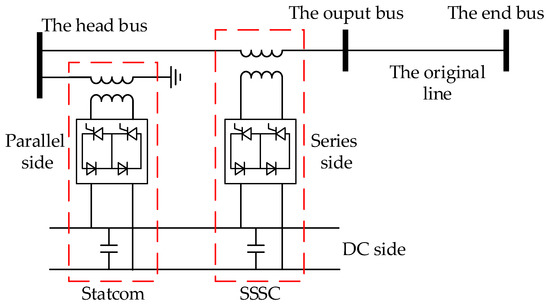
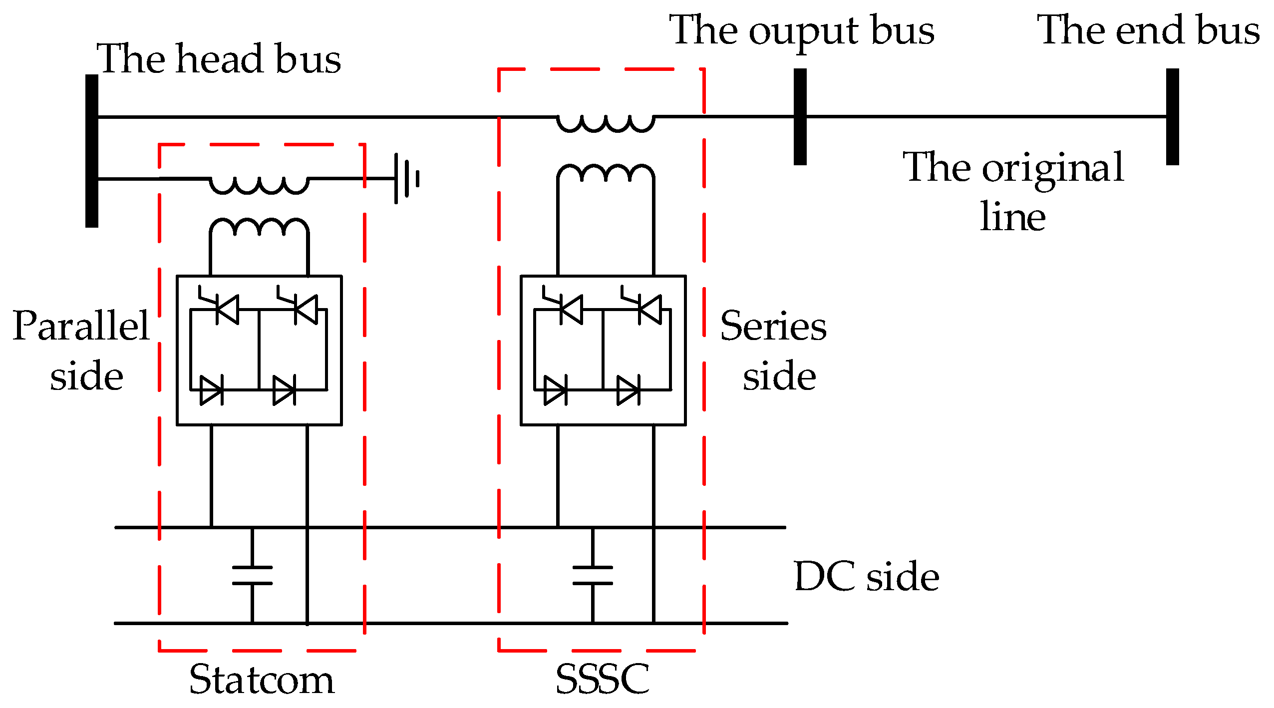
The UPFC is added to a branch, which consists of a parallel side and a series side. The parallel side is a stationary synchronous compensator (STATCOM) and the series side is a stationary synchronous series compensator (SSSC). The UPFC differs from them in that it connects STATCOM and SSSC by active power through a DC system. Thus, the UPFC possesses all the characteristics of these two devices. The basic structure of the UPFC is shown in Figure 1 [24]. It can be seen that the two sides of the UPFC are coupled through the DC system under the action of the converter through the series transformer and parallel transformer, respectively.

Figure 1. The basic structure of UPFC.

Due to the two sides of the UPFC being connected through a DC network, sufficient active power needs to be provided to the DC system from the AC system to ensure the stable operation of the whole system. In practice, the parallel side often provides enough active power to the DC system. As a rule, each converter has two independent control variables: active and reactive control variables. However, the parallel side should provide the active power, and has only one reactive control variable, which is often the connected AC bus voltage amplitude or the reactive power injection to the connected AC bus. However, the series side has two independent variables, which can control the active and reactive power of the branch, respectively. The control variables are shown in Table 1.

Table 1. The control variables of UPFC.

	The Active Control Variable	The Reactive Control Variable
The parallel side	―	The reactive power injection or the AC bus voltage amplitude
The series side	The active power	The reactive power

2.2. The Steady-State Model of UPFC

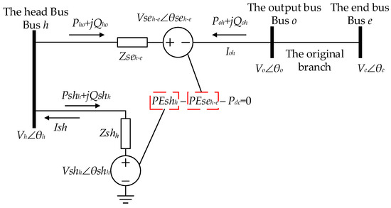
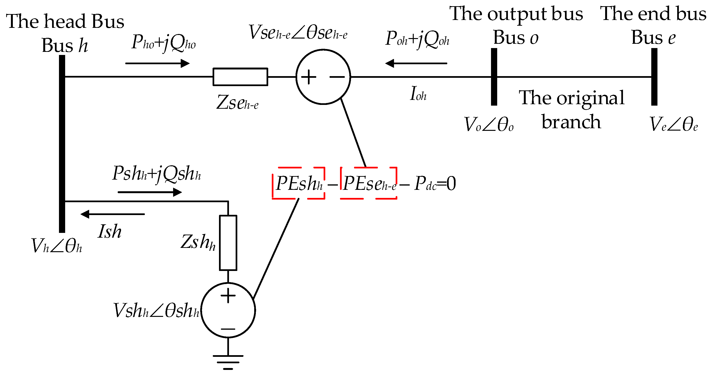
The equivalent circuit diagram of UPFC is shown in Figure 2. The parallel side is placed in the head bus, and the series side is placed between the head bus and the end bus. A virtual bus (i.e., the output bus) is used to clearly describe the relationship between physical quantities of the UPFC. In Figure 2, ${Zse}_{h-e}$ represents the equivalent impedance of the series side, and ${Zsh}_h$ represents the equivalent impedance of the parallel side. ${Vse}_{h-e}\angle \theta {se}_{h-e}$ represents the series injected voltage, and ${Vsh}_h\angle \theta {sh}_h$ represents the parallel injected voltage. It worth noting that ${Vse}_{h-e} \ge 0$ and ${Vse}_{h-e}\in \left[-\mathsf{\pi },+\mathsf{\pi }\right]$. The reference direction of voltage is shown in Figure 2.

Figure 2. The equivalent circuit diagram of UPFC.

According to the positive direction in Figure 2, we can obtain the complex power ${\stackrel{\sim }{S}}_{ho}{=P}_{ho}{+jQ}_{ho}$ from the head bus to the output bus as follows:

$$\left\{\begin{array}{l}{P}_{ho}=V_h^{2}Gs{e}_{ho}-V_h{V}_o\left[Gs{e}_{h-e}cos({\theta }_h-{\theta }_o)+Bs{e}_{h-e}sin({\theta }_h-{\theta }_o)\right]\\ -V_{h}Vs{e}_{h-e}\left[Gs{e}_{h-e}cos({\theta }_h-\theta s{e}_{h-e})+Bs{e}_{h-e}sin({\theta }_h-\theta s{e}_{h-e})\right]\\ Q_{mn}=-V_h^{2}Bs{e}_{h-e}-V_h{V}_o\left[Gs{e}_{h-e}sin({\theta }_h-{\theta }_o)-Bs{e}_{h-e}cos({\theta }_h-{\theta }_o)\right]\\ -V_{h}Vs{e}_{h-e}\left[Gs{e}_{h-e}sin({\theta }_h-\theta s{e}_{h-e})-Bs{e}_{h-e}cos({\theta }_h-\theta s{e}_{h-e})\right]\end{array}\right.$$

(1)

Similarly, the complex power ${\stackrel{\sim }{S}}_{oh}{=P}_{oh}{+jQ}_{oh}$ from the output bus to the head bus can be determined as follows:

$$\left\{\begin{array}{l}{P}_{oh}=V_o^{2}Gs{e}_{h-e}-V_o{V}_h\left[Gs{e}_{h-e}cos({\theta }_o-{\theta }_h)+Bs{e}_{h-e}sin({\theta }_o-{\theta }_h)\right]\\ +V_{o}Vs{e}_{h-e}\left[Gs{e}_{h-e}cos({\theta }_o-\theta s{e}_{h-e})+Bs{e}_{h-e}sin({\theta }_o-\theta s{e}_{h-e})\right]\\ Q_{oh}=-V_o^{2}Bs{e}_{h-e}-V_o{V}_h\left[Gs{e}_{h-e}sin({\theta }_o-{\theta }_h)-Bs{e}_{h-e}cos({\theta }_o-{\theta }_h)\right]\\ +V_{n}Vs{e}_{h-e}\left[Gs{e}_{h-e}sin({\theta }_o-\theta s{e}_{h-e})-Bs{e}_{h-e}cos({\theta }_o-\theta s{e}_{h-e})\right]\end{array}\right.$$

(2)

The complex power injection ${\stackrel{\sim }{S}sh}_h{=Psh}_h{+jQsh}_h$ from the head bus to the parallel side is as follows:

$$\left\{\begin{array}{l}Ps{h}_h=V_h^{2}Gs{h}_h-V_{h}Vs{h}_h\left[Gs{h}_{h}cos({\theta }_h-\theta s{h}_h)+Bs{h}_{h}sin({\theta }_h-\theta s{h}_h)\right]\\ Qs{h}_h=-V_h^{2}Gs{h}_h-V_{h}Vs{h}_h\left[Gs{h}_{h}sin({\theta }_h-\theta s{h}_h)-Bs{h}_{h}cos({\theta }_h-\theta s{h}_h)\right]\end{array}\right.$$

(3)

The active power ${PEsh}_h$ and ${PEse}_{h-e}$ emitted by the equivalent power source on the parallel side and series side can be shown as follows:

$$\left\{\begin{array}{c}\begin{array}{c}PEs{h}_h=Re(Vs{h}_{h}Is{h}_h^{*})\\ =Vs{h}_h^{2}Gs{h}_h-V_{h}Vs{h}_h\left[Gs{h}_{h}cos({\theta }_h-\theta s{h}_h)-Bs{h}_{h}sin({\theta }_h-\theta s{h}_h)\right]\\ PEs{e}_{h-e}=Re(Vs{e}_{h-e}{I}_{oh}^{*})\\ =Vs{e}_{h-e}^{2}Gs{e}_{h-e}-V_{h}Vs{e}_{h-e}\left[Gs{e}_{h-e}cos({\theta }_h-\theta s{e}_{h-e})-Bs{e}_{h-e}sin({\theta }_h-\theta s{e}_{h-e})\right]\\ +V_{o}Vs{e}_{h-e}\left[Gs{e}_{h-e}cos({\theta }_o-\theta s{e}_{h-e})-Bs{e}_{h-e}sin({\theta }_o-\theta s{e}_{h-e})\right]\end{array}\end{array}\right.$$

(4)

where Ish is the current injecting into the AC system from the parallel side, and ${Ise}_{oh}$ is the current flowing from bus o to bus h. In Equations (1)–(4), ${Gsh}_h{+jBsh}_h=1/{Zsh}_h$, ${Gse}_{h-e}{+jBsh}_{h-e}=1/{Zsh}_{h-e}$.

2.3. The Power Flow Calculation Method of AC System with UPFC

2.3.1. The Mismatch Equations of UPFC

As for the analysis above, four parameters, ${Vsh}_h,\theta {sh}_h,{Vse}_{h-e},\theta {se}_{h-e}$, need to be solved in a UPFC. Therefore, it is necessary to build four independent equations.

For the series side, there are two control parameters. They are the active power $P_{h-e}^{ref}$ and the reactive power $Q_{h-e}^{ref}$ of the series branch. According to these, two equations can be built as follows:

$$\left\{\begin{array}{l}\Delta P_{h-e}=P_{oh}+P_{h-e}^{ref}\\ \Delta Q_{h-e}=Q_{oh}+Q_{h-e}^{ref}\end{array}\right.$$

(5)

As for the parallel side, there is one independent controlled quantity. That is the AC bus voltage amplitude $V_h^{ref}$ or the reactive power injection to the AC bus to which the UPFC parallel side is connected. If the parallel side controls the AC bus voltage amplitude, the equation can be written as follows:

$$\Delta V_h=V_h-V_h^{ref}$$

(6)

Furthermore, the active power balance should be satisfied between the parallel and series sides of the UPFC, as follows:

$$\Delta PE=PEs{h}_h-PEs{e}_{h-e}-P_{dc}=0$$

(7)

In general, $P_{dc} \approx 0$.

2.3.2. The Mismatch Equations of the AC System

In the AC system, the mismatch equations ΔP and ΔQ about the power injection are often written. As for the buses which are not connected to the UPFC (the buses except bus h and o in Figure 2), the regular mismatch equations can be written as follows:

$$\left\{\begin{array}{c}\Delta P_i=P_i-U_i{\displaystyle {\sum }_j{U}_j(G_{ij}cos{\theta }_{ij}+B_{ij}sin{\theta }_{ij})}\\ \Delta Q_i=Q_i-U_i{\displaystyle {\sum }_j{U}_j(G_{ij}sin{\theta }_{ij}-B_{ij}cos{\theta }_{ij})}\end{array}\right.$$

(8)

where $G_{ij}{ \mathrm{and} B}_{ij}$ represent the real and imaginary part of the corresponding elements of the nodal admittance matrix, respectively, while the phase angle deviation between the two buses ${\theta }_{ij}{=\theta }_i-{\theta }_j$.

If the bus is connected to the UPFC, the mismatch equations should be changed to the following:

$$\left\{\begin{array}{c}\Delta P_i=P_i-U_i{\displaystyle {\sum }_j{U}_j(G_{ij}cos{\theta }_{ij}+B_{ij}sin{\theta }_{ij})-P_k}\\ \Delta Q_i=Q_i-U_i{\displaystyle {\sum }_j{U}_j(G_{ij}sin{\theta }_{ij}-B_{ij}cos{\theta }_{ij})-Q_k}\end{array}\right.$$

(9)

where

$$P_k=\left\{\begin{array}{l}Ps{h}_h+P_{ho}\hspace{0.33em}\\ P_{oh}\\ 0\end{array}\right.,Q_{UPFC,k}=\left\{\begin{array}{l}Qs{h}_h+Q_{ho} ,k\in h\\ Q_{oh}\hspace{0.17em} ,k\in o\\ 0\hspace{0.17em}\hspace{0.17em} ,k\in \mathrm{others}\end{array}\right.$$

(10)

2.3.3. The Power Flow Calculation Method of the AC System with UPFC

According to all the mismatch equations established above, the solution equations for the AC system with UPFC by Newton Raphson method can be written as follows:

$$\mathit{F}=-\mathit{J}\Delta \mathit{X}$$

(11)

where $\mathit{X}= {\left[{\mathit{X}}_{\mathrm{AC}}^T{, \mathit{X}}_{\mathrm{UPFC}}^T\right]}^T$, ${\mathit{X}}_{AC}$ represents the AC bus voltage amplitude and phase angle, ${\mathit{X}}_{AC}={[\theta , V]}^T$. ${\mathit{X}}_{UPFC}$ represents the variables of the UPFC, ${\mathit{X}}_{UPFC}={\left[{\theta }_{sh}, V_{sh}, {\theta }_{se}, V_{se}\right]}^T$. Furthermore, $\mathit{F}= {\left[{\mathit{F}}_{\mathrm{AC}}^T{, \mathit{F}}_{\mathrm{UPFC}}^T\right]}^T$, ${\mathit{F}}_{AC}$ represents the unbalance equations of the bus power injection of the AC system, ${\mathit{F}}_{AC}={\left[\Delta P, \Delta Q\right]}^T$.${ F}_{UPFC}$ represents the unbalance equations of the UPFC, ${\mathit{F}}_{UPFC}={\left[{\Delta P}_{h-e}{, \Delta Q}_{h-e}{, \Delta V}_h, \Delta PE\right]}^T$. $\mathit{J}=\partial \mathit{F}/\partial \mathit{X}$ represents the system Jacobian matrix, as follows:

$$\mathit{J}=\left[\begin{array}{cc}\frac{\partial {\mathit{F}}_{AC}}{\partial {\mathit{X}}_{AC}}& \frac{\partial {\mathit{F}}_{AC}}{\partial {\mathit{X}}_{UPFC}}\\ \frac{\partial {\mathit{F}}_{UPFC}}{\partial {\mathit{X}}_{AC}}& \frac{\partial {\mathit{F}}_{UPFC}}{\partial {\mathit{X}}_{UPFC}}\end{array}\right]$$

(12)

3. The Basic Theories of LHS-MCS

3.1. The Principles of the LHS Method

The sampling technique is a key step in the Monte Carlo simulation method. The traditional random sampling Monte Carlo simulation method (RS-MCS) requires a large number of samples to accurately describe the probability characteristics of random variables. However, increasing the sample size will inevitably increase the total simulation time and greatly reduce computational efficiency. Obviously, decreasing sample size can effectively reduce the calculation time under the condition of ensuring accuracy. The Latin hypercube sampling (LHS) is a typical stratified sampling method. Compared to the normal random sampling method, the Latin hypercube sampling method can cover a larger sampling space of random input variables with the same sampling size.

Ronald L. Iman points out that for the same sampling size N, the expected values of the joint coverage space of two independent random variables obtained, respectively, by random sampling and Latin hypercube sampling are as follows [25]:

$$\mathrm{RS}:{\left[\left(N-1\right)/\left(N+1\right)\right]}^2\times 100\% \mathrm{LHS}:{\left[\left(N-1\right)/N\right]}^2\times 100\%$$

(13)

When $\mathrm{N} \ge 2$, the value of the latter is always larger than the value of the former, so the sampling space of the random input variable covered by the Latin hypercube sampling is always larger than that of the random sampling on the premise of an identical sample size.

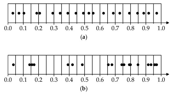
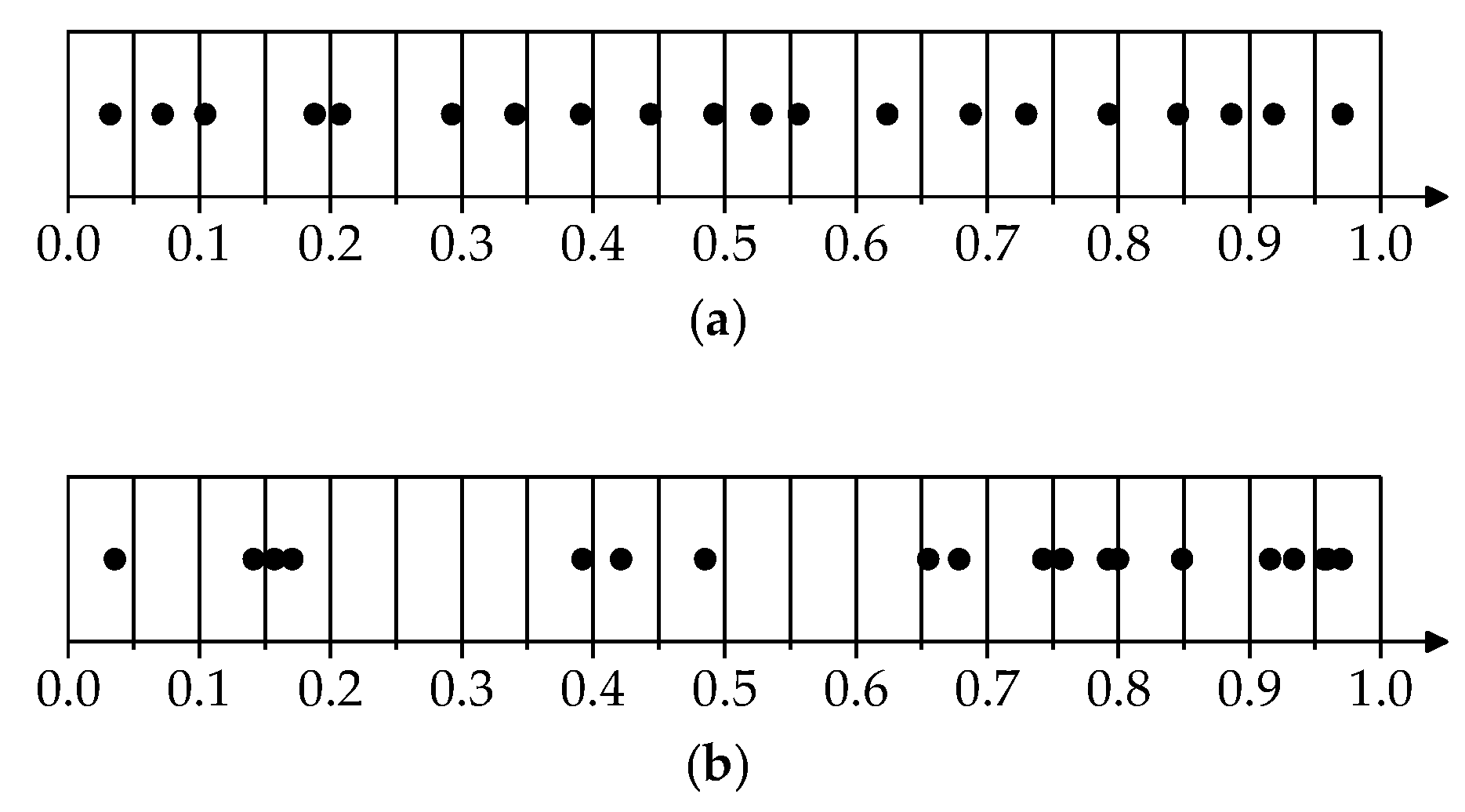
To more vividly present the performance differences between the LHS and RS methods, Figure 3 shows the distribution of uniform sampling of the identical sample size (the sampling interval is 0–1, and the number of sampling points is 20). From this figure, it can be seen that the LHS method has only one sampling point in each sampling interval, which can obtain a more uniform sampling distribution, while the results obtained by the RS method are more disordered. In other words, when the number of sampling points is the same, the sampling results of the LHS method can better reflect the distribution of the original input variables. This also illustrates the advantage that LHS can conduct stratified sampling.

Figure 3. Schematic comparison of the LHS and RS methods: (a) LHS method; (b) RS method.

The LHS method mainly consists of two steps: sampling and sorting.

3.1.1. The Sampling

The sampling step of the LHS method is to make sure that the samplings can fully cover the distribution areas of the random input variables.

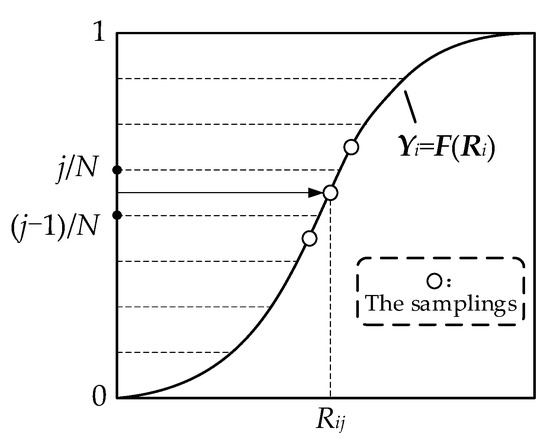
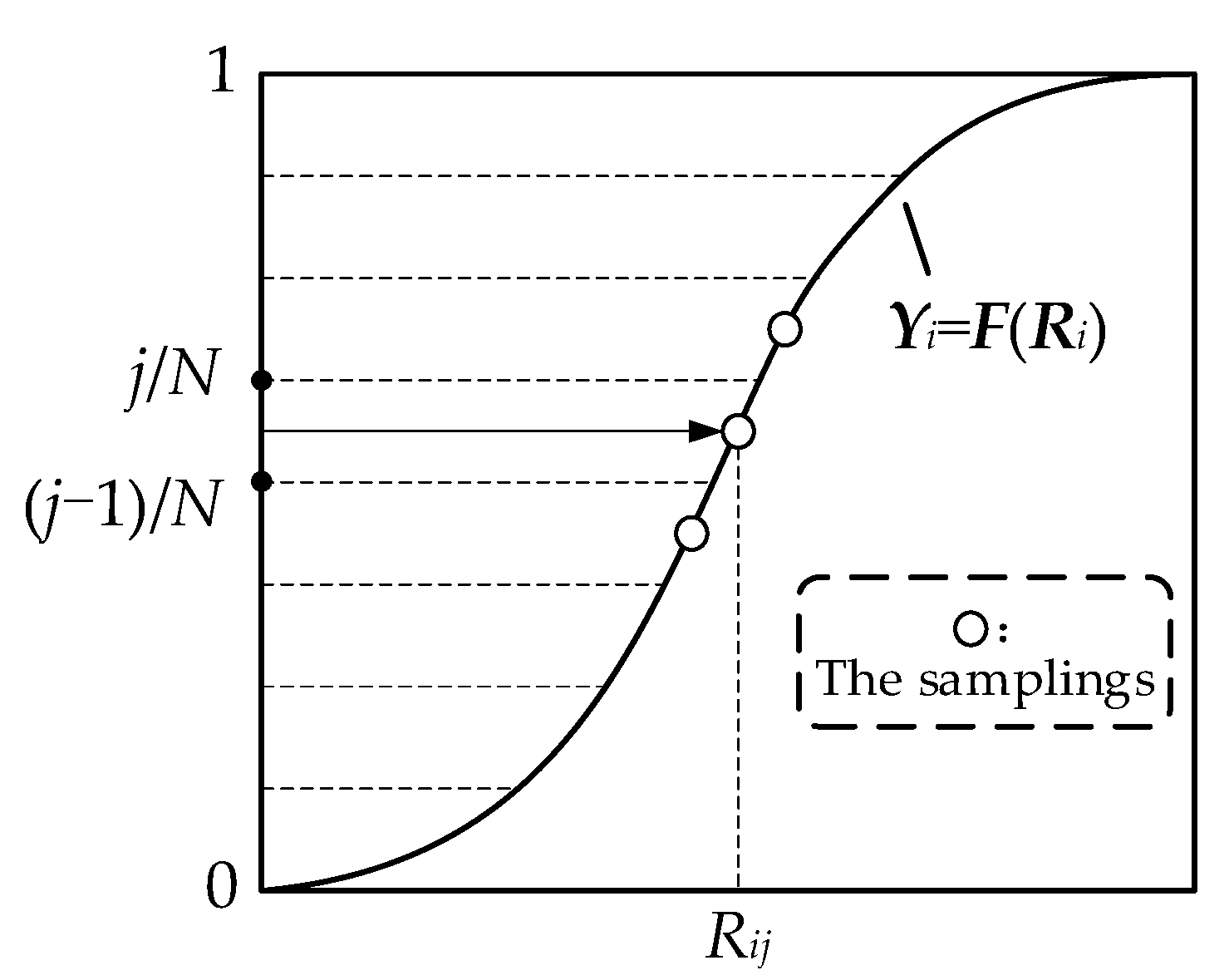
The K-dimensional random variable ${\mathit{R}}_{K\times N}$ satisfying a certain distribution is ${[\mathit{R}}_1{, \mathit{R}}_2{, \dots , \mathit{R}}_i{, \dots ,\mathit{R}}_K]$. The cumulative density function (CDF) F that the variable satisfies is $\mathit{Y}=\mathit{F}\left(\mathit{R}\right)$. If the sampling size is set to N for the random variable of the i-th dimension, the sampling value is ${{[R}_{i1}{, R}_{i2}{, \dots , R}_{ij}{, \dots , R}_{iN}]}^T$. At the same time, N non-overlapping equally spaced intervals can be provided as $[0, 1/N]$, $[1/N, 2/N]$, …, $\left[\right(N-1)/N, 1]$. The length of each interval is $1/N$. When picking a number from each interval, the data set about $Y_i$ can be obtained as ${{[Y}_{i1}{, Y}_{i2}{, \dots , Y}_{ij}{, \dots , Y}_{iN}]}^T$.

There are three different picking methods: interval random sampling (IRS), importance sampling (IS), and lattice sampling (LS). Because of the high sampling efficiency and good robustness of the lattice sampling, it is used in this paper. The principle of the LS method is to take the midpoint of each interval, and then the j-th sampling of $R_i$ can be obtained as follows:

$$R_{ij}=F^{-1}\left[(j-0.5)/N\right]$$

(14)

where $F^1$ is the inverse function of F.

The sampling diagram of the lattice is shown in Figure 4.

Figure 4. The sampling diagram of the LHS method.

3.1.2. The Sorting

The correlation between different random input variables after the sampling is uncontrollable, which will affect the quality and accuracy of the subsequent data processing. However, the sorting is to ensure that the correlation of samplings tends to be minimized by changing the arrangement. Thus, the generated low-correlation variable matrix is used as the basis for the subsequent variable space.

The correlation between the rows of the sampling matrix ${\mathit{R}}_{K\times N}$ can be measured by a $K\times K$ correlation coefficient matrix ρ, which can be expressed as follows:

$$\mathit{\rho }=\left\{{\rho }_{ij}\hspace{0.33em}\hspace{0.33em}\hspace{0.33em}i=1,2,\dots ,K;j=1,2,\dots ,K\right\}$$

(15)

where ${\rho }_{ij}$ is the correlation coefficient between the data in row i and row j of R, expressed as follows:

$${\rho }_{ij}=\frac{{\displaystyle \sum _{k=1}^N\left[\left(R_{ik}-{\overline{R}}_i\right)\left(R_{jk}-{\overline{R}}_j\right)\right]}}{\sqrt{{\displaystyle \sum _{k=1}^N{\left(R_{ik}-{\overline{R}}_i\right)}^2{\displaystyle \sum _{k=1}^K{\left(R_{jk}-{\overline{R}}_j\right)}^2}}}}$$

(16)

The sorting methods mainly include the Cholesky decomposition method, Gram–Schmidt sequence orthogonalization method, genetic algorithm, and so on. For random variables with correlation, the correlation between the samplings of random variables can be satisfied as far as possible by sorting.

For the Cholesky decomposition method, the main idea is to reduce the correlation by constructing an approximately orthogonal arrangement matrix ${\mathit{L}}_{K\times N}$ to rearrange the positions of data in the sampling matrix, while the value of each data point remains the same. The value of each row of the arrangement matrix L represents the permutation position of the corresponding data of the sampling matrix R. The steps for constructing the permutation matrix by Cholesky decomposition are as follows:

• Set the initial value of L; each row consists of a random permutation of the set of integers [1, 2, …, N].
• By using the Cholesky decomposition method to decompose the correlation coefficient matrix ρ, a lower trigonometric matrix D can be obtained, which satisfies ${\mathit{\rho }=\mathit{D}\mathit{D}}^T$.
• Obtain a sort matrix with a lower column correlation as ${\mathit{L}’=\mathit{D}}^{-1}\mathit{L}$. It is worth noting that the elements in $\mathit{L}’$ may not be positive integers, so each row of data in $\mathit{L}’$ can be arranged in order from largest to smallest and reassigned to positive integers ranging from 1 to N.
• Repeat steps 1 to 3 until the column correlation of L is less than a predetermined value. Then, according to the arrangement order, which can be represented in L, R is arranged to obtain the final sampling matrix.

3.2. The Procedure for LHS-MCS

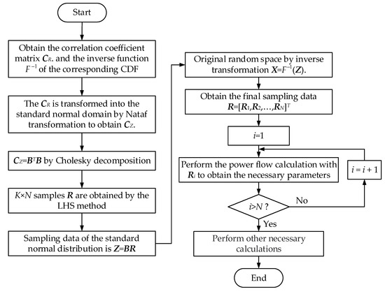
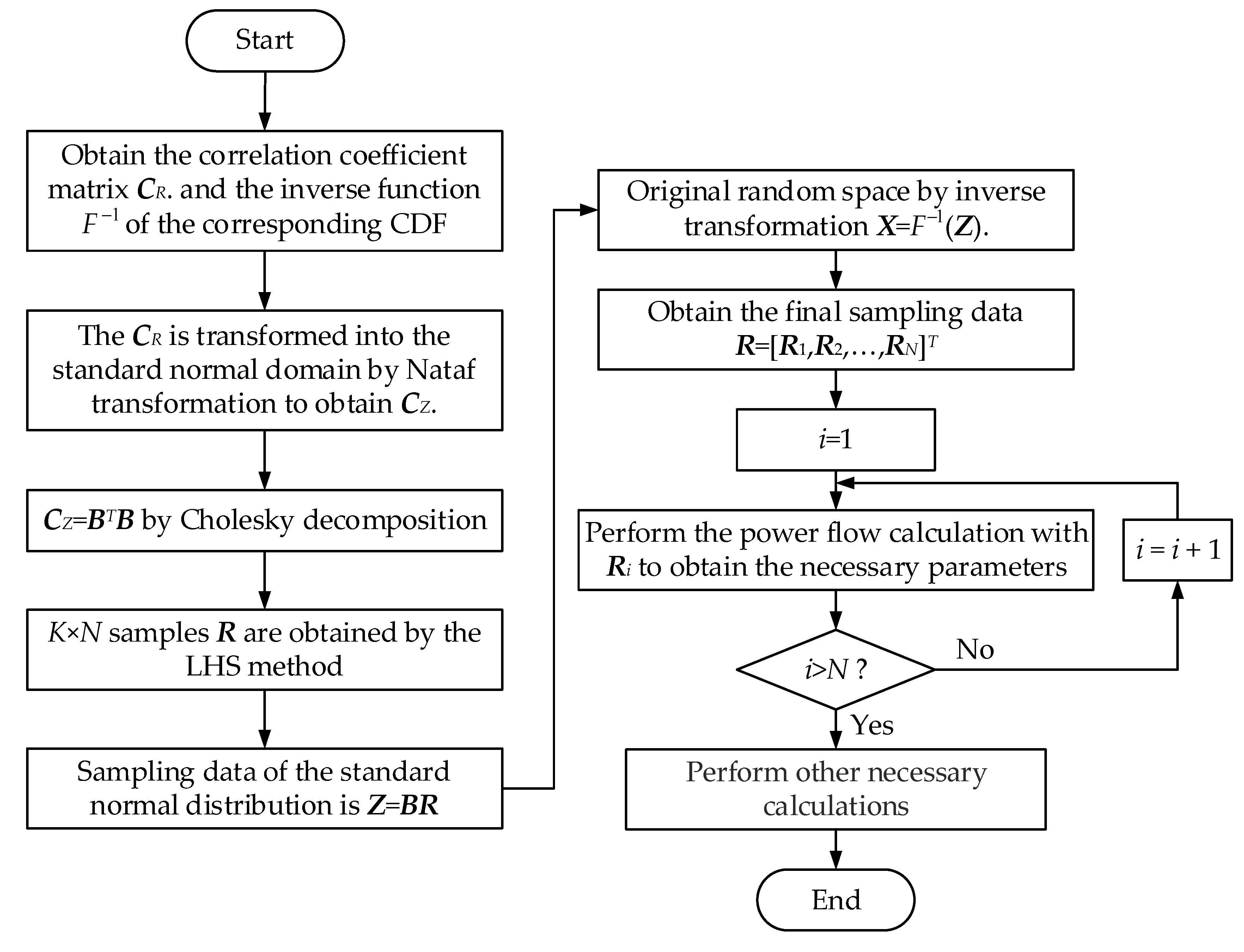
In probabilistic scenarios, the input variables tend to be correlated. For example, wind farms in the same region have similar wind speeds. Thus, the wind speeds in this region are strongly correlated. However, different input variables may satisfy different probability distributions, so it is difficult to deal with the inputs that are correlated and follow different distributions by using conventional methods. Furthermore, the Nataf transformation is a powerful tool to deal with such kinds of problems. It can establish the relationship between any distribution and the normal distribution that the correlated random input variables follow. At the same time, the Nataf transformation can transform the correlation coefficients of any two variables that satisfy an arbitrary distribution into the correlation coefficients of two variables in the Gaussian domain. Therefore, the correlation relationship of all variables can be obtained in the Gaussian domain. Additionally, the correlated random variables satisfying the correlation can be generated in the Gaussian domain and then transformed into the original domain for subsequent calculations. In fact, the Nataf transformation is a computationally intensive process, but it is not the focus of this paper. For one of the calculation methods, please refer to [26]. In this paper, the LHS-MCS combined with the Nataf transformation is employed to solve the PPF problem. The specific computational steps of the method are shown in Figure 5.

Figure 5. Flow chart of the specific PPF calculation steps combining Nataf transformation and LHS-MCS.

4. Probabilistic Determination on the Power Flow Entropy and Available Load Supply Capability

4.1. Definition of Some Indices

4.1.1. Improved Power Flow Entropy

To quantify the equilibrium of power flow distribution, the index of power flow entropy is derived. Firstly, the loading rate of the branch i-j is defined as follows:

$${\beta }_{i-j}=\frac{P_{i-j}}{P_{i-j}^{max}}$$

(17)

where $P_{i-j}$ represents the active power transmitted by the branch i-j in the current deterministic scenario. $P_{i-j}^{\max }$ represents the active power capacity of the branch i-j.

Set an equal-difference column:$C=\left[C_1{, C}_2{, \dots , C}_k{, C}_{k+1}{, \dots , C}_n\right]$, $C_n=1$. The equal difference is $\Delta {C=C}_{k+1} -{ C}_k$. In this paper, $\Delta C=0.05$. Now the number of loading rates in the interval $\left[\left.C_k{, C}_{k+1}\right)\right.$ can be calculated as ${\mu }_k$. Repeat this step until all the intervals of the loading rate have been calculated. Then, the proportion of the number of branches in the k-th interval to the number of all the branches can be obtained as follows:

$$P(k)=\frac{{\mu }_k}{{\displaystyle {\sum }_{j=1}^{n-1}{\mu }_j}}$$

(18)

Correspondingly, the traditional power flow entropy ${\eta }_{\mathrm{Tr}}$ can be obtained as follows:

$${\eta }_{\mathrm{Tr}}=-C{\displaystyle {\sum }_{k}P(k)lnP(k)}$$

(19)

where C is a constant, and usually ln10.

However, the power flow entropy calculated by Equation (19) only shows the distribution of active power of each branch, without considering the loading rate of each branch. If it is necessary to study the loading rate of the system based on the equilibrium of power flow; thus, the improved power flow entropy η should be adopted:

$$\eta =-C{\displaystyle {\sum }_k\omega (k)P(k)lnP(k)}$$

(20)

where $\omega \left(k\right)$ represents the average loading rate of the branches whose loading rates are in the interval $\left[\left.C_k{, C}_{k+1}\right)\right.$. Furthermore, $\omega \left(k\right)$ can be calculated by the following equation:

$$\omega (k)=\frac{{\displaystyle {\sum }_{\mathsf{\beta }\in \left[{\mathrm{C}}_{\mathrm{k}},{\mathrm{C}}_{\mathrm{k}+1}\right)}\beta }}{{\mu }_k}$$

(21)

From Equation (20), it can be determined that a smaller η does not only indicate a more reasonable power flow distribution in the system, but also indicates that the loading rate of each branch is higher, and the branch capacity is better utilized in the current condition. For the safe, stable, and economical operation of the power system, a smaller η should be obtained.

4.1.2. Available Load Supply Capability

The max-multiple of the load added to the power system can be used to represent the ALSC. Furthermore, the degree of the load growth can be quantified by the load-increasing multiple λ. The max-multiple ${\lambda }_{\max }$ can be obtained by gradually increasing λ while satisfying the system limits. Evidently, the larger ${\lambda }_{\max }$ is, the larger the available load supply capacity is. Therefore, ${\lambda }_{\max }$ can be used to measure ALSC effectively. In this paper, the active power transmission capacity of each branch is limited. Furthermore, the active and reactive power of each bus gradually increases until certain limits are violated. The objective is to find ${\lambda }_{\max }$, which aims to determine the ALSC of the system. The above can be described mathematically as follows.

The objective:

$$\mathrm{m}\mathrm{a}\mathrm{x}\hspace{0.33em}\hspace{0.33em}\lambda$$

(22)

Subject to:

$$\left\{\begin{array}{l}\mathit{F}=f({\mathit{X}}_{(0)})+(\lambda -1)(P_{(0)}+j{Q}_{(0)})\\ {\beta }_{i-j}\le 1\end{array}\right.$$

(23)

where $f\left(\mathit{X}\right)$ is the physical equation for the initial state of the system. $P_{\left(0\right)}$ represents the active power injection, and $Q_{\left(0\right)}$ represents the reactive power injection at the initial state of the power system.

4.2. The Repeated Power Flow

To solve the ALSC under the DPF, the RPF calculation can be used. The basic principle of RPF calculation is that, starting from the basic state of the system, λ is gradually increased. Repeatedly calculate the power flow until the constraints are not satisfied. At this time, the ${\lambda }_{\max }$ of the system can be obtained. That is, the available load supply capacity of the system has been determined.

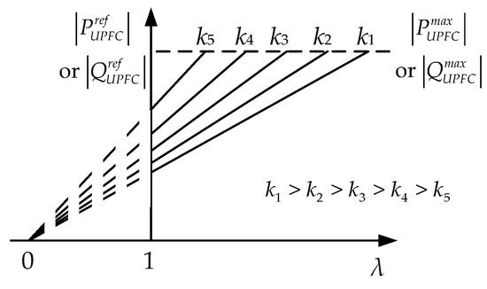
In the process of repeated power flow calculation, λ is going to keep increasing. If the control parameters of the UPFC are also kept constant, this will be detrimental to the system power flow. If the actual transmission power of one branch is small, but the transmission power of this branch becomes larger through the control of the UPFC, the transmission power of other branches may exceed the limit. This may lead to the system falling out of safety and causing other serious problems. When this happens in the process of the RPF calculation, the calculation might not converge or can give the wrong results. Therefore, it is necessary to adjust the control parameters of the UPFC during the RPF calculation. The notion of the UPFC control coefficient k is introduced here. The relationship between the control parameters of the UPFC and the control coefficient k can be represented as follows:

$$\left\{\begin{array}{l}\left|P_{UPFC}^{ref}\right|=(\left|P_{h-e}^{max}\right|-0.05)\times \frac{\lambda }{k}=\left|P_{UPFC}^{max}\right|\times \frac{\lambda }{k}\\ \left|Q_{UPFC}^{ref}\right|=\left|Q_{UPFC}^{max}\right|\times \frac{\lambda }{k}\end{array}\right.$$

(24)

where $P_{UPFC}^{ ref}$ and $Q_{UPFC}^{ ref}$ represent the current setting active and reactive power of the UPFC series side, respectively. $P_{h-e}^{ \max }$ represents the active power capacity where the series side of UPFC is located. $P_{UPFC}^{ \max }$ and $Q_{UPFC}^{ \max }$ represent the maximum setting of active and reactive power on the series side of UPFC.

Under different control coefficients k, the control values of UPFC with the changes in λ are shown in Figure 6.

Figure 6. The changes in the UPFC control variables under different control coefficients.

However, the key point is how to obtain ${\lambda }_{\max }$. The conventional approach is to determine a step h first. For each calculation, the values of active power and reactive power increase by h. A large h may lead to a high-speed calculation but a lower calculation accuracy, while a smaller h may lead to a higher calculation accuracy but a slower calculation speed. Therefore, it is necessary to select a proper h that does not cost too much computing time while having relatively higher computational accuracy. Given this, a new method with variable h is proposed. The procedure of RPF with the change in step h and the UPFC control variables is as shown below:

• Import basic system data. Set the initial values of h. Set $\lambda =1$ At this time, the load of each bus is ${P+jQ=P}_{\left(0\right)}{+jQ}_{\left(0\right)}$. The UPFC control parameters are $P_{UPFC}^{ref}{=P}_{UPFC}^{max}/k$ and $Q_{UPFC}^{ref}{=Q}_{UPFC}^{max}/k$.
• Calculate the power flow of the system and determine whether the active power of each branch exceeds the capacity. If no, turn to step 3; if yes, turn to step 4.
• Perform $\lambda =\lambda +h$, $P+jQ=\lambda (P+jQ)$, $P_{UPFC}^{ref}{=P}_{UPFC}^{max}\lambda /k$, and $Q_{UPFC}^{ref}{=Q}_{UPFC}^{max}\lambda /k$. Then, go back to step 2.
• Perform $\lambda =\lambda + h$, and order $h=h/2$. Judge whether h is smaller than the convergence accuracy. If yes, go to Step 5; if no, go back to step 2.
• Perform other necessary calculations and give out the results.

4.3. The Step of the PRPF

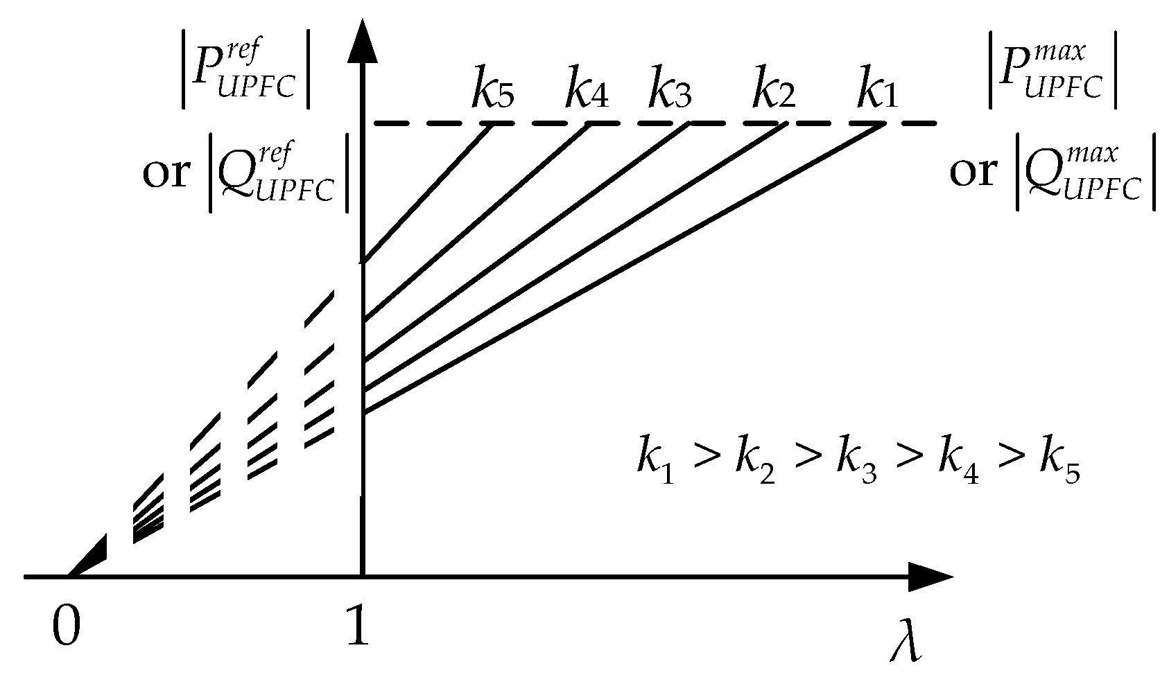
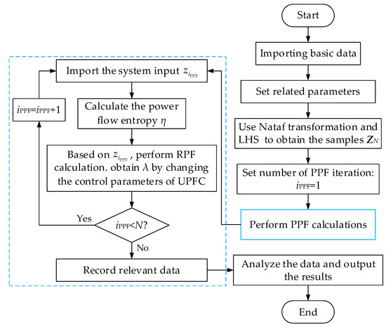
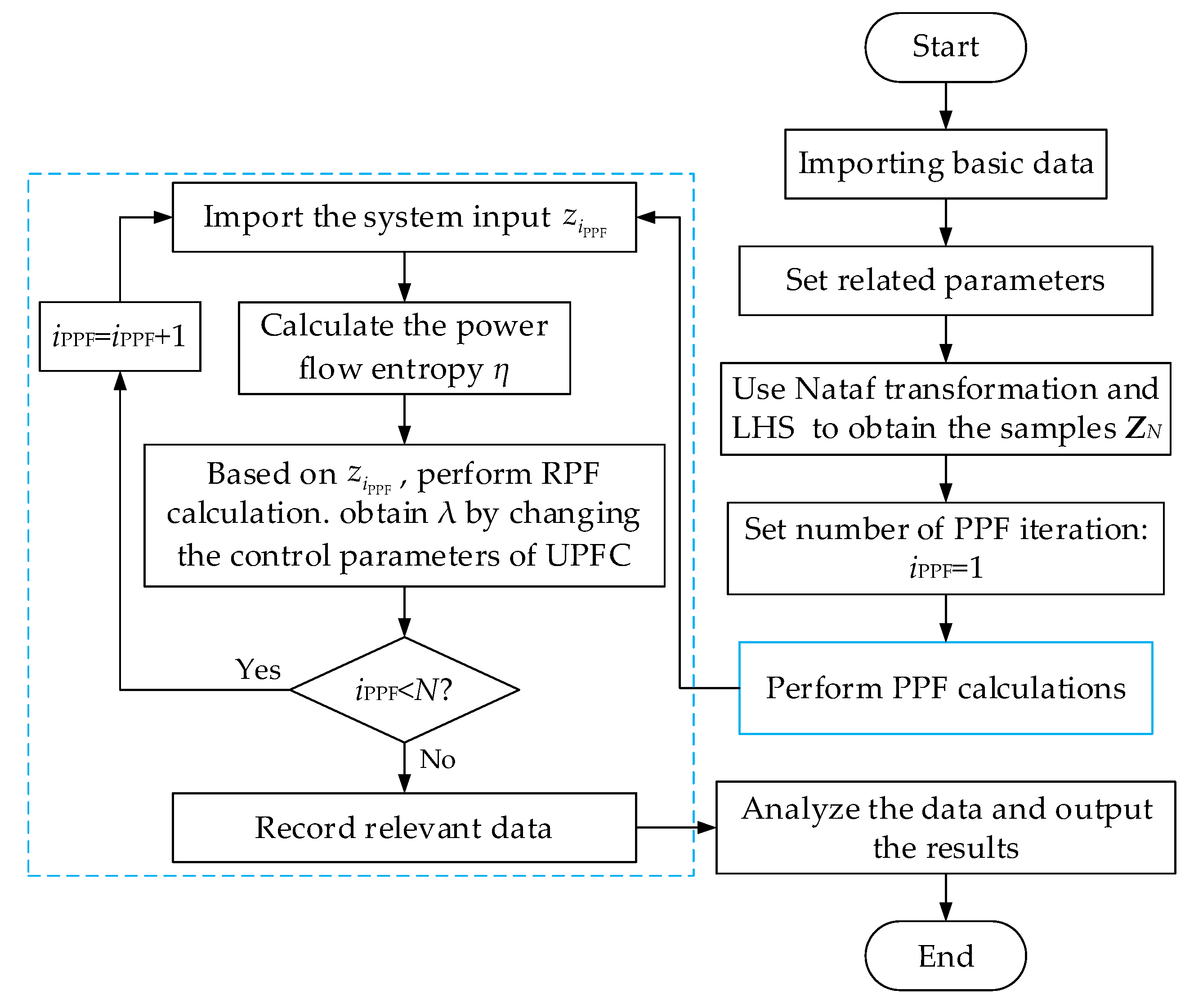
In this paper, considering the control of UPFC under the probabilistic scenarios, the relationship between the η at the initial state and ${\lambda }_{\max }$ of each probabilistic scenario is deeply studied. This is obviously a process combining PPF calculation and RPF calculation (i.e., PRPF). The specific calculation steps are shown in Figure 7. In this figure, generate the matrix Z_N of samplings through the LHS method and Nataf transformation, in which there are N groups of samplings. That is, ${\mathbf{Z}}_N{=[z}_1{, z}_2{, \dots , z}_{i_{PPF}}{, \dots , z}_N]$. Set the iteration of probabilistic power flow calculation as i_PPF, then for the i_PPF-th probabilistic power flow calculation, the system input of each probabilistic power flow calculation is $z_{i_{\mathrm{P}\mathrm{P}\mathrm{F}}}$. Then, based on $z_{i_{\mathrm{P}\mathrm{P}\mathrm{F}}}$, the power flow entropy η and λ can be calculated.

Figure 7. Flow chart of the PRPF calculation based on the LHS-MCS method.

5. Test Results

5.1. The DPF Calculation of AC System with UPFC

To assess the performance of the proposed steady-state model, Case A, based on a modified IEEE 14-bus system, is designed. The base power is set to 100 MVA. The active power output of the generator at bus 2 is modified to 0.65 p.u. and that of the generator at bus 6 is modified to 0.85 p.u.. In addition, the active power capacity of each branch is set as shown in Table 2.

Table 2. The active power capacity of each branch.

Branch	1–2	1–5	2–3	2–4	2–5	3–4	4–5
Pmax/p.u.	3	1.5	1.5	1.5	2	1.5	2
Branch	4–7	4–9	5–6	6–11	6–12	6–13	7–8
Pmax/p.u.	1	1	1	1	1	1	1
Branch	7–9	9–10	9–14	10–11	12–13	13–14
Pmax/p.u.	1	1	1	1	1	1

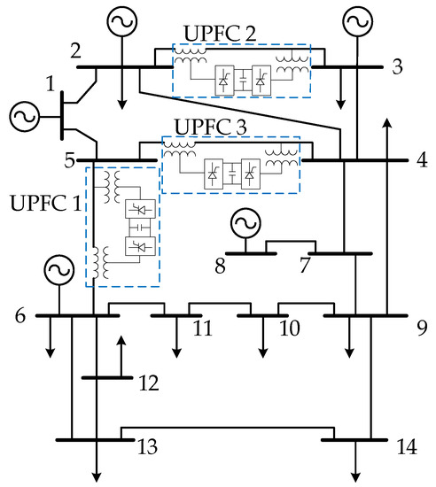
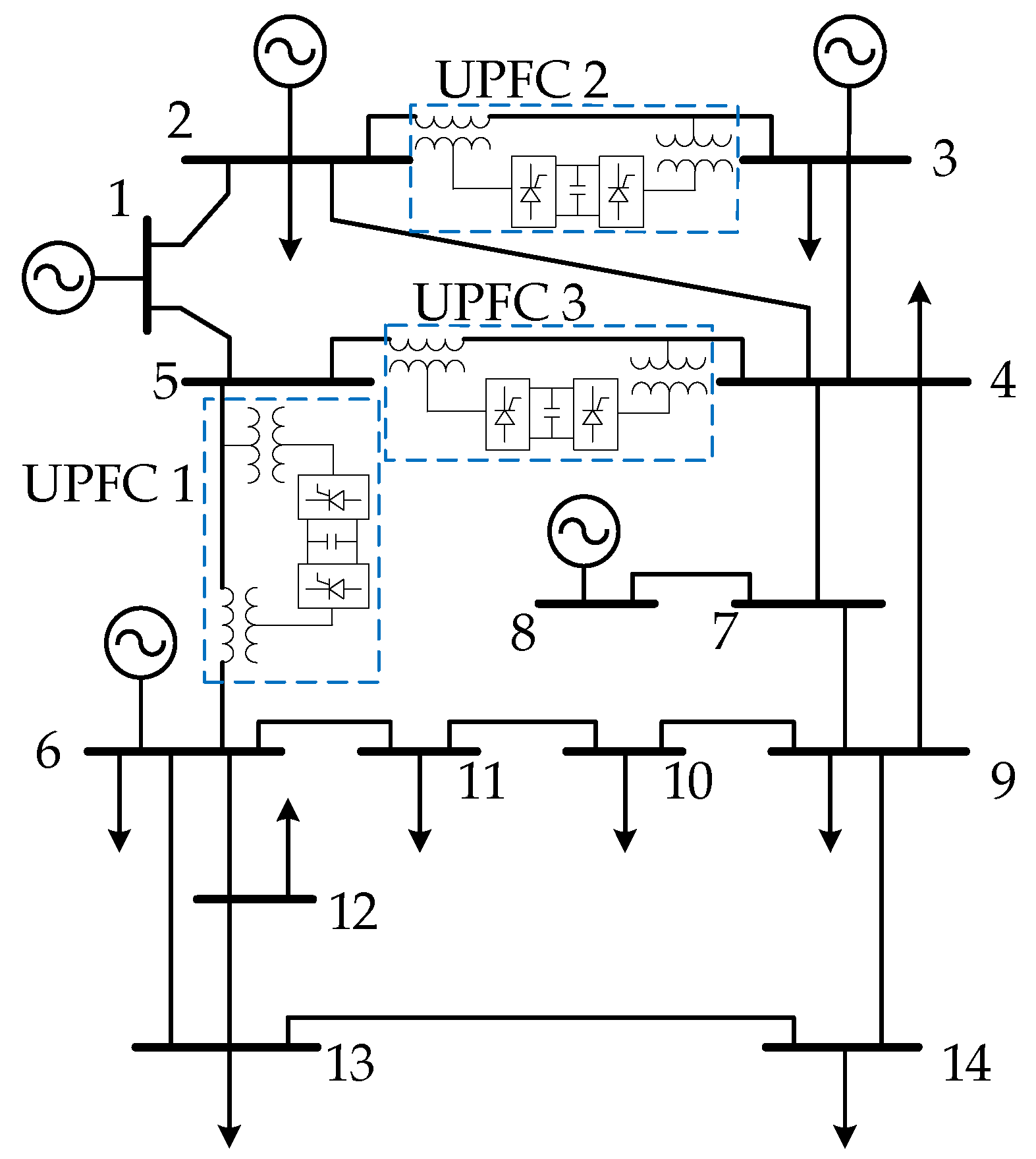
Three UPFCs are added. The equivalent impedance of the UPFC is $Zsh=Zse=0+j0.1$. Table 3 describes the UPFC control parameters. The modified IEEE 14-bus system after adding three UPFCs is shown in Figure 8. The head buses of each UPFC are buses 5, 2, and 4, respectively. The output buses of each UPFC are buses 6, 3, and 5, respectively. The convergence coefficient of the DPF calculation is set as ${10}^{-6}$.

Table 3. The settings on the control parameters of UPFC.

	Parallel Side/p.u.	Series Side/p.u.
UPFC1	$V_5^{ref}=1.02$	${\tilde{S}}_{5-6}^{ref}=-0.3+j0.2$
UPFC2	$V_2^{ref}=1.03$	${\tilde{S}}_{2-3}^{ref}=0.8+j0.4$
UPFC3	$V_4^{ref}=0.98$	${\tilde{S}}_{4-5}^{ref}=-0.7+j0.3$

Figure 8. The modified IEEE 14-bus system with three UPFCs.

5.1.1. Validity of the Proposed Model of UPFC

Based on the above basic data, it can be determined that the whole calculation converges after six times, and the running time is 0.01 s.

The calculation results of UPFC parameters are shown in Table 4.

Table 4. The calculation results of UPFC.

UPFC1	Vse5-6	θse5-6	Vsh5	θsh5
	0.1580	1.6738	0.9950	−0.0577
UPFC2	Vse2-3	θse2-3	Vsh2	θsh2
	0.1529	−2.4690	1.0231	−0.0321
UPFC3	Vse4-5	θse4-5	Vsh4	θsh4
	0.1008	2.2749	0.9395	−0.0923

Note: the unit of Vse and Vsh is p.u., and that of θse and θsh is rad.

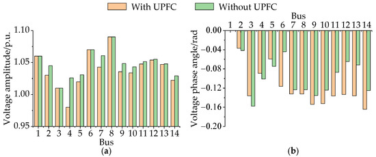
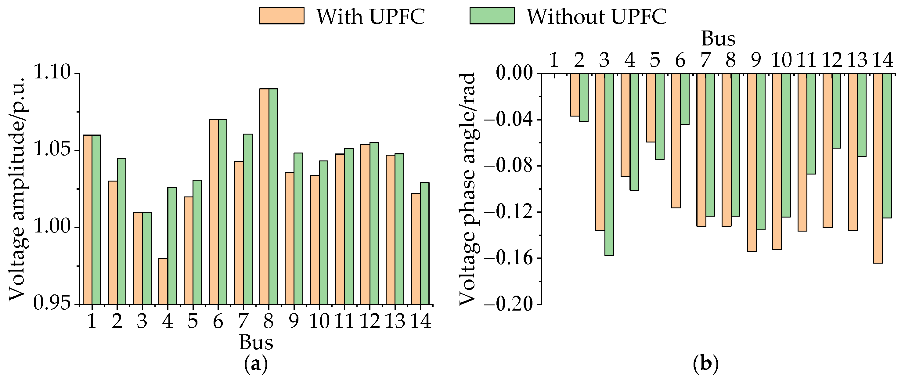
Meanwhile, the comparison of the voltage amplitude and phase angle of the AC system before and after adding the UPFC can be obtained from Figure 9. From the figure, it can be seen that the voltage amplitude of buses 2, 4, and 5 remains at the set value, as mentioned in Table 3. The voltage amplitudes and phase angles of other buses have some variations after adding the UPFC to the AC system.

Figure 9. The comparison on voltage amplitude and voltage phase angle with or without UPFC: (a) The comparison on voltage amplitude; (b) The comparison on voltage phase angle.

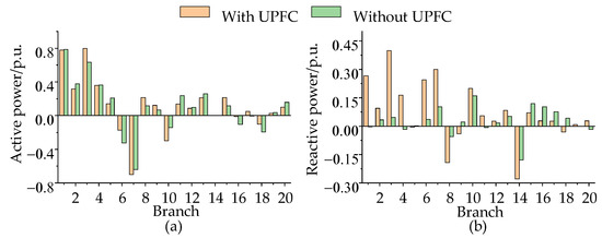
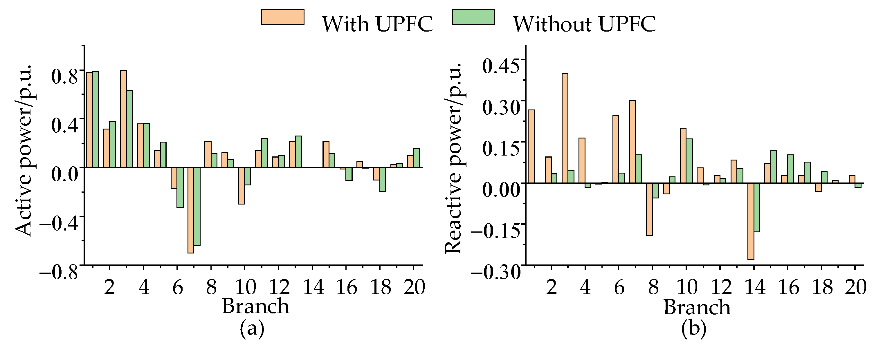
Figure 10 shows the comparison of active power and reactive power of each branch of the AC system before and after adding the UPFC. From the figure, it can be seen that the power of branches 2–3, 4–5, and 5–6 (i.e., branches 3, 7, and 10 in Figure 10) remains at the set value mentioned in Table 3. In addition, the power flow of the whole system has changed significantly.

Figure 10. The comparison between active and reactive power for each branch with or without UPFC: (a) The comparison on active power; (b) The comparison on reactive power.

Therefore, from these two figures above, it can be seen that UPFC can indeed control the power flow and change the physical quantities in the AC system. The power flow entropy η can be calculated to be 3.4878 by Equation (20). In general, it is clear that the steady-state model of UPFC established in this paper can be used for the DPF calculation of the AC system with UPFC.

5.1.2. Robustness of the Proposed Algorithm

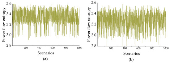
To verify the robustness of the deterministic power flow calculation principles and algorithms for AC systems with UPFC in this paper, the power injection of the bus is changed to make the load randomly fluctuate up and down by 10% around the basic value (subject to the uniform distribution) when the UPFC parameters are fixed. Furthermore, the control parameters of UPFC are randomly changed up and down by 10% around the basic value (also subject to the uniform distribution) when the load is fixed. The line graph shown in Figure 11 reflects the results of power flow entropy under different conditions. A total of 1000 load cases are generated in Figure 11a, 1000 UPFC control parameter cases are generated in Figure 11b, and then the respective 1000 results of power flow entropy η are determined.

Figure 11. Robustness verification of the system with UPFC when the loads and control parameters of UPFC change: (a) The loads change; (b) The control parameters of UPFC change.

As shown in Figure 11, the power flow calculation is convergent in all 1000 scenarios (1000 groups of reasonable power flow entropies are obtained) no matter the change in the loads or the control parameters of UPFC. Furthermore, for the 1000 calculations, it takes only about 3.5 s. Thus, the regulation ability of UPFC for the system is tested, and the robustness of the model is verified. At the same time, due to the high efficiency of calculation, a lot of time can be saved in the subsequent procedure of probabilistic power flow calculation.

5.2. Tests of Combining LHS-MCS and Repeated Power Flow

5.2.1. Test System under Study

This section mainly studies the η of the initial state and ALSC of each probabilistic scenario. These random scenarios (e.g., Case B1) are established based on the deterministic cases used above. The uncertainties of the load follow the normal distribution, the mean value is the original basic data, and the standard deviation is 5% of the mean value. All loads are assumed to have a constant power factor, that is, the power factor remains constant throughout the active power change. The correlation coefficient of every two loads is set to 0.2.

At the same time, the wind farms are added to buses 6, 9, 10, and 13, and the numbers of wind turbines are 13, 7, 14, and 21, respectively.

In addition, the relationship between the active power output P of the wind turbine and the wind speed v is as follows:

$$P=\left\{\begin{array}{l}2(v-4)/11 4\le v\le 15\hfill \\ 2 15\le v\le 25 \hfill \\ 0 \mathrm{else}\hfill \end{array}\right.$$

(25)

The unit of P is MW, and that of v is m/s.

The wind speed in the area where the wind farms are located follows the Weibull distribution with the proportional parameters $\alpha =10.7$ and shape parameters $\mathsf{\beta }=3.97$. Meanwhile, there is a strong correlation between the wind speeds of each wind farm, and the correlation coefficient matrix is as follows:

$$\begin{array}{l}\begin{array}{ccccc}& 1& 2& 3& 4\end{array}\\ R=\begin{array}{c}1\\ 2\\ 3\\ 4\end{array} \left[\begin{array}{cccc}1& 0.88& 0.87& 0.91\\ 0.88& 1& 0.85& 0.87\\ 0.87& 0.85& 1& 0.85\\ 0.91& 0.87& 0.85& 1\end{array}\right]\end{array}$$

(26)

Set the maximum control parameters of the three UPFCs, as shown in Table 5. The control coefficient k is set to 2, while the specific control parameters of UPFC can be obtained by Equation (24).

Table 5. The setting of AC node voltage amplitude and branch maximum power of UPFC.

	Parallel Side/p.u.	Series Side/p.u.
UPFC1	$V_5^{ref}=1.045$	${\tilde{S}}_{5-6}^{max}=-0.95+j0.2$
UPFC2	$V_2^{ref}=1$	${\tilde{S}}_{2-3}^{max}=1.45+j0.1$
UPFC3	$V_4^{ref}=1.07$	${\tilde{S}}_{4-5}^{max}=-1.95+j0.2$

To verify the performance of the LHS-MCS method under different scenarios, Case B1 is taken as the basis, and the other five cases (Case B2~Case B6) are designed for comparison. These cases are shown in Table 6.

Table 6. Different probabilistic scenarios related to the basic case.

Case	Modification
Case B1	Basic case
Case B2	Basic case but not including UPFC
Case B3	Change the standard deviation of each load from 5% to 15%
Case B4	Change the standard deviation of each load from 5% to 25%
Case B5	Change the correlation coefficient between loads from 0.2 to 0.5
Case B6	Change the correlation coefficient between loads from 0.2 to 0.8

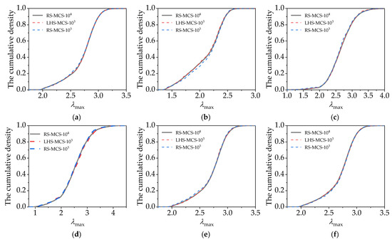
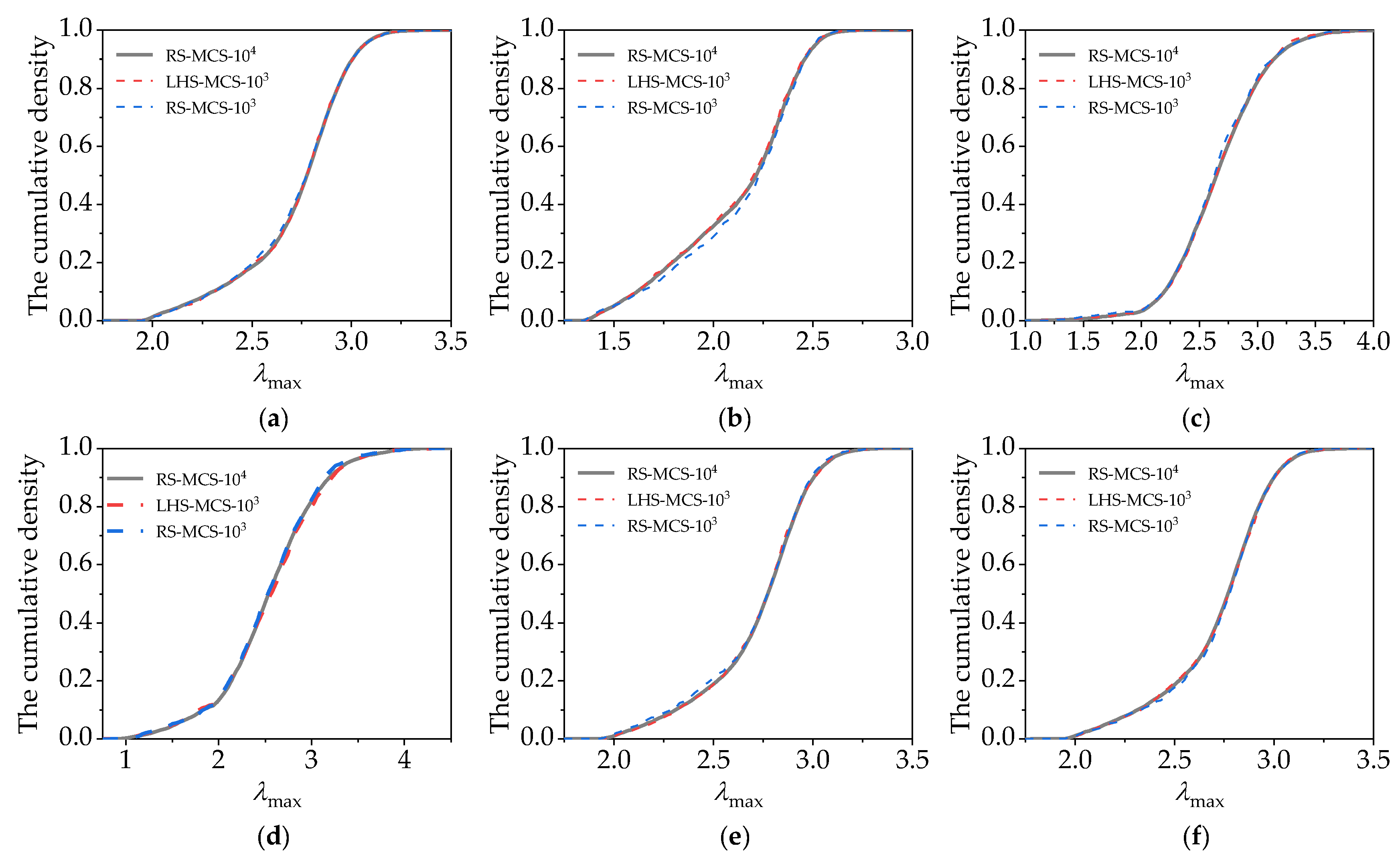
The results of the RS-MCS method are used as the reference data and compared with the LHS-MCS method. The sampling number of the RS-MCS method is set to 10000 and 1000 (i.e., RS-MCS-10⁴ and RS-MCS-10³), and that of the LHS-MCS is set to 1000 (i.e., LHS-MCS-10³). The results of RS-MCS-10⁴ are regarded as the reference. The convergence criterion of the repeated power flow calculation is assigned as ${10}^{-3}$.

5.2.2. Analysis of the Results

Through the calculation of Case B1~Case B6, it can be obtained that the average calculation time of RS-MCS-10⁴ is 2497.6 s, while that of LHS-MCS-10³ and RS-MCS-10³ is about 248 s.

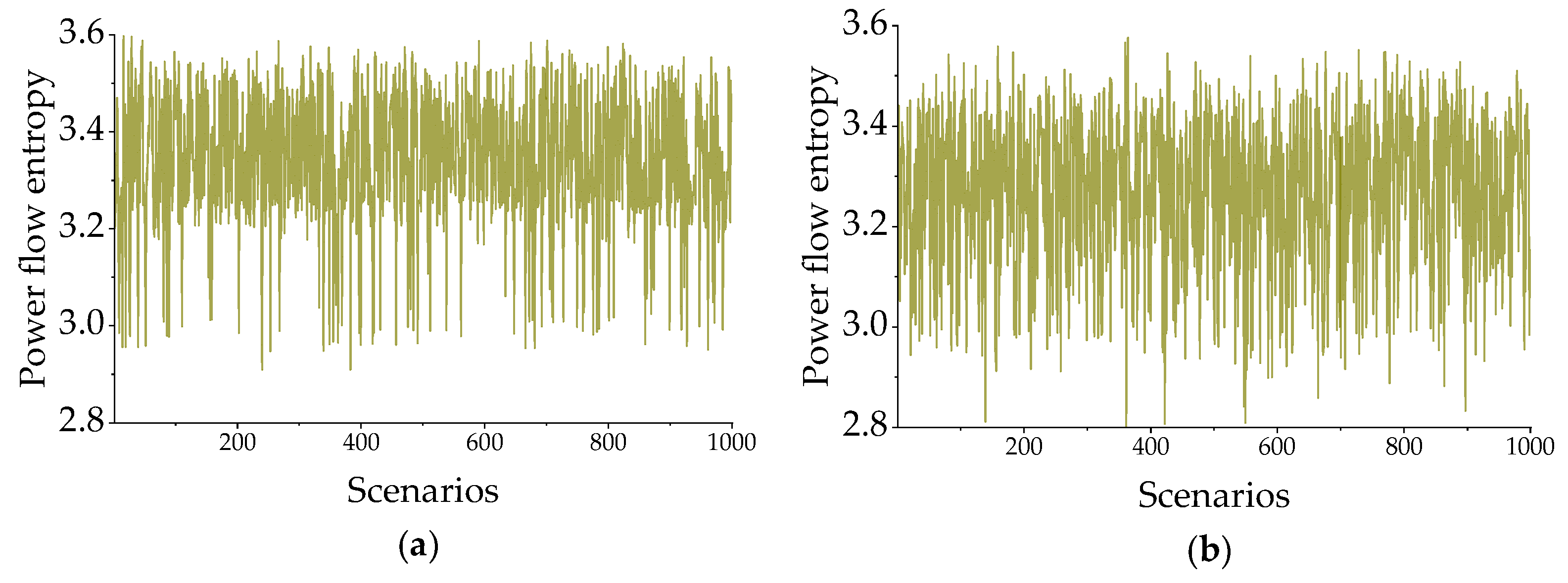
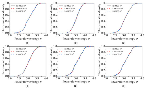
Under different cases, the cumulative density function (CDF) of η and ${\lambda }_{\max }$ by PRPF method based on LHS-MCS-10³, RS-MCS-10³, and RS-MCS-10⁴ are obtained, as shown in Figure 12 and Figure 13, respectively.

Figure 12. The CDF of power flow entropy η: (a) Case B1; (b) Case B2; (c) Case B3; (d) Case B4; (e) Case B5; (f) Case B6.

Figure 13. The CDF of ${\lambda }_{\max }$: (a) Case B1; (b) Case B2; (c) Case B3; (d) Case B4; (e) Case B5; (f) Case B6.

It can be seen from the figure that in each group of experiments, the cumulative density curves calculated by the two methods are basically in coincidence. Thus, it is proved that LHS-MCS has a higher calculation accuracy.

From the figure, the cumulative density curves calculated by the three methods are approximate in each case. However, it is evident that compared to RS-MCS-10³, the curve calculated by LHS-MCS-10³ is closer to the curve calculated by RS-MCS-10⁴. Therefore, it is proven that LHS-MCS has higher computational accuracy.

At the same time, the mean and variance relative errors of η and ${\lambda }_{\max }$ can be obtained by using LHS-MCS-10³ and RS-MCS-10³ under different cases, which are shown in Table 7. The relative error is calculated by the following Equation (27):

$${\delta }_{\mu }=\left|\frac{{\mu }_{\mathrm{LHS}/\mathrm{RS}-\mathrm{MCS}-10^3}-{\mu }_{\mathrm{RS}-\mathrm{MCS}-10^4}}{{\mu }_{\mathrm{RS}-\mathrm{MCS}-10^4}}\right|....{\delta }_{{\sigma }^2}=\left|\frac{{\sigma }_{\mathrm{LHS}/\mathrm{RS}-\mathrm{MCS}-10^3}^2-{\sigma }_{\mathrm{RS}-\mathrm{MCS}-10^4}^2}{{\sigma }_{\mathrm{RS}-\mathrm{MCS}-10^4}^2}\right|$$

(27)

where ${\delta }_{\mu }$ and ${\delta }_{{\sigma }^2}$ represent the relative errors in calculating the mean and variance of each index, respectively. ${\mu }_{{\mathrm{LHS}/\mathrm{RS}-\mathrm{MCS}-10}^3}$ represent the mean values of the results calculated by LHS-MCS-10³ or RS-MCS-10³. ${\sigma }_{{\mathrm{LHS}/\mathrm{RS}-\mathrm{MCS}-10}^3}^2$ represent the variances in the results calculated by LHS-MCS-10³ or RS-MCS-10³.

Table 7. The mean and variance relative error of power flow entropy η and ${\lambda }_{\max }.$

			Case B1	Case B2	Case B3	Case B4	Case B5	Case B6
η	Mean	LHS-MCS-103	1.87 × 10−4	3.29 × 10−4	1.63 × 10−3	2.33 × 10−3	4.49 × 10−4	6.44 × 10−4
		RS-MCS-103	7.98 × 10−3	5.03 × 10−3	2.59 × 10−3	3.51 × 10−3	3.04 × 10−3	1.61 × 10−3
	Variance	LHS-MCS-103	7.98 × 10−3	1.25 × 10−2	1.98 × 10−2	1.41 × 10−2	3.11 × 10−2	5.53 × 10−2
		RS-MCS-103	5.30 × 10−2	4.17 × 10−2	7.85 × 10−3	6.12 × 10−2	1.64 × 10−2	1.00 × 10−1
${\lambda }_{\max }$	Mean	LHS-MCS-103	1.91 × 10−5	3.46 × 10−3	1.13 × 10−3	2.10 × 10−3	5.63 × 10−4	5.75 × 10−4
		RS-MCS-103	1.81 × 10−3	8.73 × 10−3	6.65 × 10−3	6.88 × 10−3	4.62 × 10−3	2.61 × 10−3
	Variance	LHS-MCS-103	4.25 × 10−3	1.54 × 10−2	4.05 × 10−3	4.60 × 10−4	2.24 × 10−3	8.07 × 10−3
		RS-MCS-103	2.37 × 10−1	4.06 × 10−2	2.02 × 10−2	1.67 × 10−2	6.89 × 10−2	2.91 × 10−2

It can be concluded from the above data that, when calculating PPF based on the LHS-MCS method, adopting fewer samplings can also guarantee high calculation accuracy and save a lot of time. From the above analysis, the LHS method can be used in the probabilistic power flow calculation of the AC system with UPFC. Therefore, in the subsequent calculation, the LHS-MCS method is used to study the related problems.

5.3. The Positive Impact of UPFC on the System under Probabilistic Scenarios

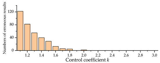
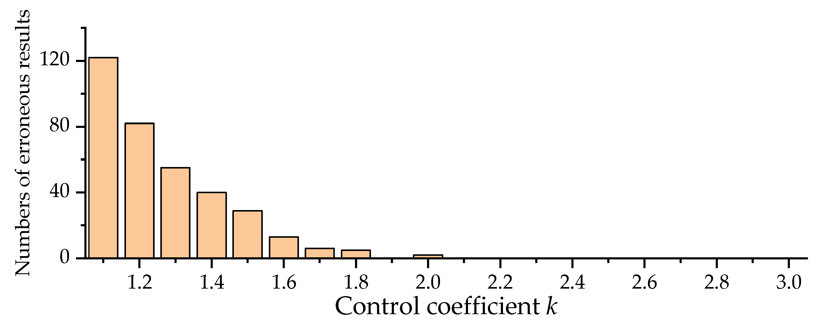
To analyze the relationship between the power flow entropy of the initial state and the available load supply capability of each sampling, Case C is set up to experiment by analyzing the operating state of the system under different control coefficients. The probabilistic scenario of Case C is the same as that of Case B1. Furthermore, in Case C, the control coefficient k is adjusted from small to large (1.1~3.0). In fact, when the control coefficient k is small, the power flow calculation may not converge. The relationship between the control coefficient and the numbers of non-convergence of the power flow can be obtained and shown in Figure 14. In Case C, the sampling size of LHS-MCS is 1000 as well.

Figure 14. The non-convergent numbers of power flow under different control coefficient k values.

As indicated in Figure 14, when k is small, the number of non-convergences of the power flow is large (the total calculation times corresponding to each value of k is 1000). As k increases, the number of non-convergence times of the power flow decreases significantly. The reason for the non-convergence of power flow analysis is as follows: when k is small, the active and reactive power of the branches controlled by UPFC changes only slightly in the process of load change and maintains a large value at any time. In other words, when the load of each bus is still at the basic level, the control transmission power of related branches is already at a large value, resulting in the chaos of the power flow distribution of the whole system, which makes the active power of some branches exceed the limits all the time. This results in a non-convergent power flow calculation. Therefore, it becomes clearly necessary to select a reasonable k so that the number of non-convergence times of the system power flow can be effectively reduced.

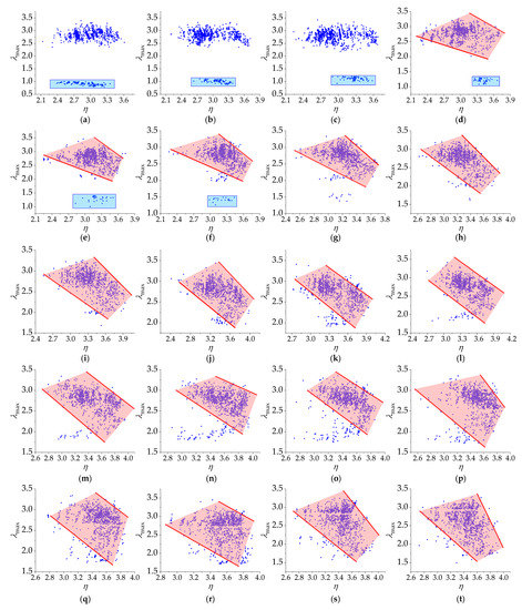
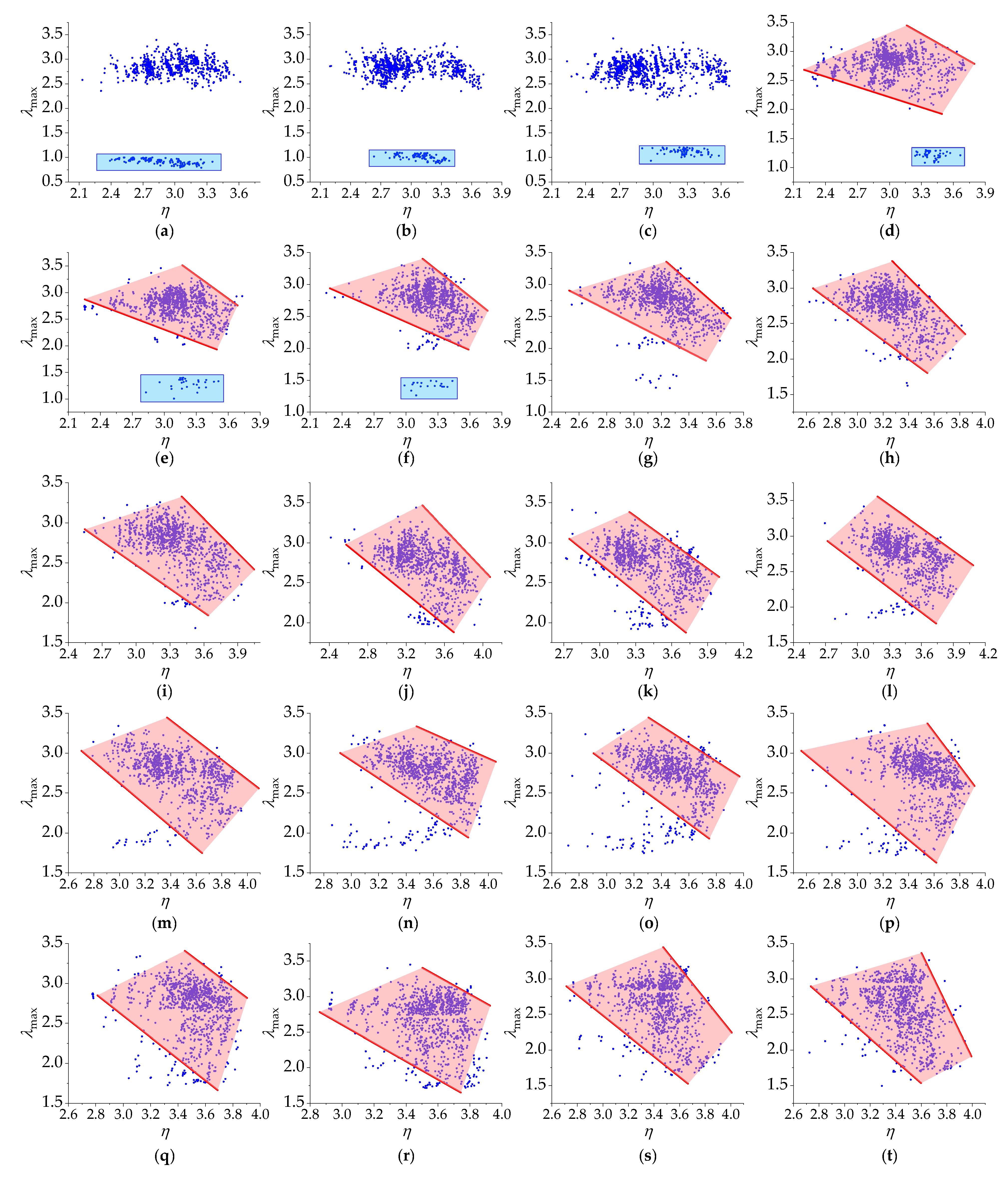
After removing the results which are not convergent, the relationship between the η of the initial state and the ${\lambda }_{\max }$ capability under a series of different control coefficients can be obtained in terms of the scatter plot, as shown clearly in Figure 15.

Figure 15. The relationship between the η of the initial state and the ${\lambda }_{\max }$ under different control coefficients: (a) k = 1.1; (b) k = 1.2; (c) k = 1.3; (d) k = 1.4; (e) k = 1.5; (f) k = 1.6; (g) k = 1.7; (h) k = 1.8; (i) k = 1.9; (j) k = 2.0; (k) k = 2.1; (l) k = 2.2; (m) k = 2.3; (n) k = 2.4; (o) k = 2.5; (p) k = 2.6; (q) k = 2.7; (r) k = 2.8; (s) k = 2.9; (t) k = 3.0.

As can be seen from the red part of Figure 15, for most of the UPFC control coefficients, ${\lambda }_{\max }$ generally decreases with the increase in the η of the initial state. That is, a smaller η often corresponds to a larger available load supply capability. The analysis of the reason can be interpreted as follows: with the increase in the system load, it is bound to cause the transmission power of each branch to increase. If the η of the initial state is smaller, it indicates that the power flow of the system is more rational, and the branch loading rate is lower at this condition. Correspondingly, with the increase in the system load, it is less likely that a certain branch will quickly increase its capacity. The power system is more capable of supporting such an increase in load. Therefore, the system would have more available load supply capability. In addition, as can be seen from the blue box in Figure 15a–f, when k is small, there exist some scenarios where the values of ${\lambda }_{\max }$ are small. In other words, under these k values, the ASLC of the system is small, which is not conducive to the secure operation of the power system.

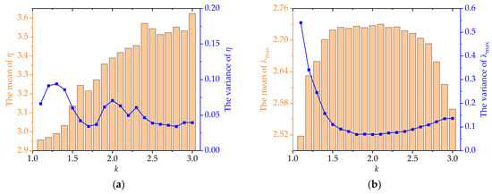
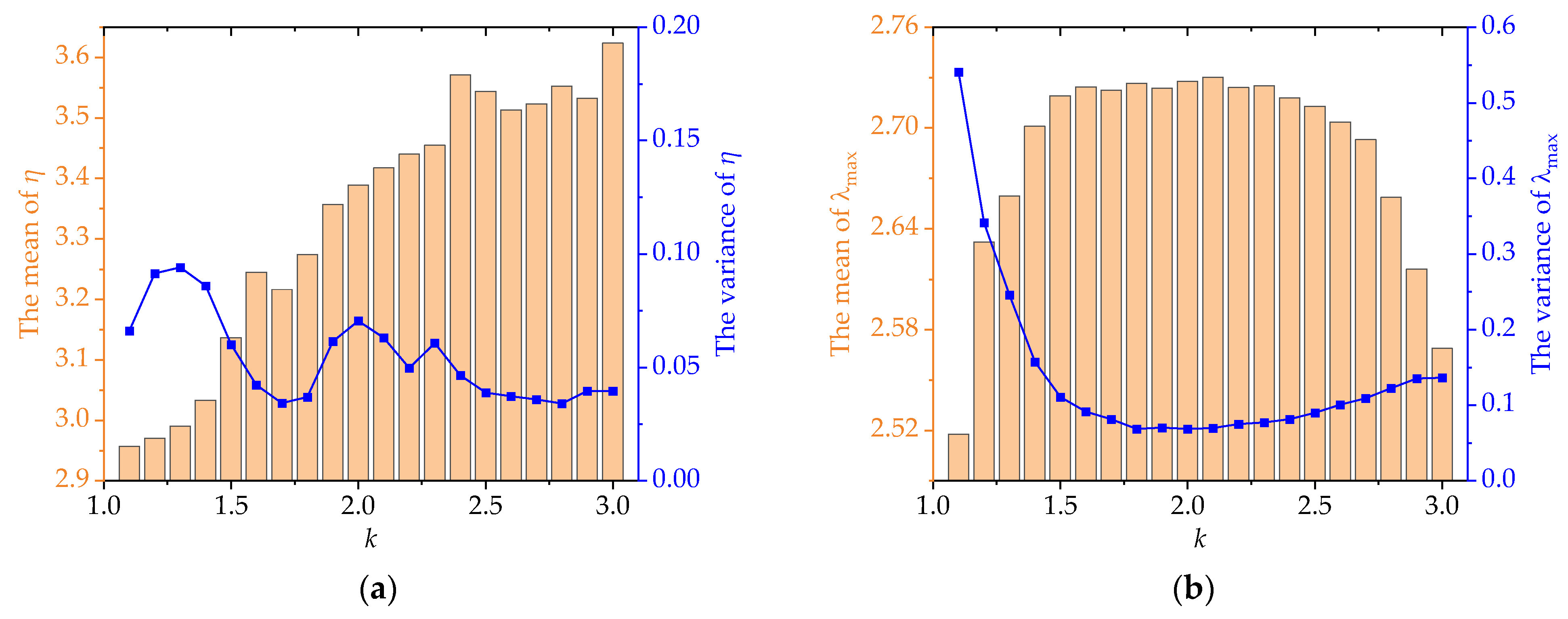
In addition, under different control coefficients, the mean and variance of η and ${\lambda }_{\max }$ are recorded and investigated, and are shown in Figure 16 below.

Figure 16. The mean and variance of the η and ${\lambda }_{\max }$ with different control coefficients: (a) The mean and variance of the η; (b) The mean and variance of the ${\lambda }_{\max }$.

As can be seen from (a) in Figure 16, the η at the initial state has different values with the changes in k. Generally, with the growth of k, the mean value of the η keeps increasing. As can be seen from (b) in Figure 16, with the growth of k, the mean value of the ${\lambda }_{\max }$ first increases and then it starts to decrease.

When k = 1.1~1.4, the η is small, but as previously analyzed, the power flow calculation will encounter the non-convergence issue more frequently. Corresponding to (b) in Figure 16, the mean values of ${\lambda }_{\max }$ of these situations are small, the variance values are large, and the ${\lambda }_{\max }$ has a wide range of fluctuations.

When k is larger, the mean value of η at the initial point is larger, and ${\lambda }_{\max }$ is also smaller. It can be seen that when k = 1.8, 1.9, and 2.1, the mean and variance of the η are relatively small, indicating that the power flow at the initial state of the system is relatively reasonable. When k = 2.0, although the variance of the η at this time is large, the mean value of the η is very small, so the power flow distribution of the system is in a relatively good balance. Accordingly, when k = 1.8, 1.9, 2.0, and 2.1, the mean value of ${\lambda }_{\max }$ is relatively larger and the variance value is smaller, indicating that when the control coefficients are assigned to these values, the system can have a larger available load supply capability.

The above analysis shows that under the UPFC control parameters, the η at the initial state is smaller, which indicates that the power flow distribution of the initial state is more rational, and the available load supply capability of the system is larger. Therefore, it is necessary to adjust the control coefficient of UPFC to make the η at the initial state smaller for ensuring the stable operation of the power system. According to the test results herein, k = 1.8, 1.9, 2.0, and 2.1 can be considered as good options for the control parameters of UPFC.

6. Conclusions

The basic structure and control strategy of UPFC are introduced first. Furthermore, the steady-state model of UPFC and the solution method of the unified iterative method are constructed and presented. The MCS method based on the LHS sampling is adopted, in which LHS is used for the sampling, and the Cholesky decomposition method is used for the sorting. The detailed steps for solving the PPF problem with LHS-MCS are formulated. Meanwhile, the improved power flow entropy index and ALSC based on the branch loading rates are defined. By using RPF calculation with variable step size, the detailed procedure for calculating the power flow entropy at the initial state and ALSC of each sampling is given. In the process of the PRPF calculation, the control parameters of the UPFC are flexibly changed by setting a control coefficient. Finally, the modified IEEE14 test system is used to analyze the accuracy and effectiveness.

The results indicate that the UPFC can effectively control the power flow of the system in the DPF scenarios, and the proposed algorithm has good robustness. Under the stochastic scenarios, it is proved that compared to the RS-MCS method, the LHS-MCS method can achieve higher accuracy while significantly reducing computational time, resulting in computational efficiency improvement of PRPF. Finally, through different values of k of UPFC, it is found that when the control coefficient is small, the number of non-convergences is significantly higher. For most control coefficients, a smaller power flow entropy at the initial state corresponds to a larger ALSC. This reveals that by controlling the UPFC, the system can have a larger ALSC while ensuring a more balanced power flow distribution in the power system. At the same time, the test results confirm that an appropriate k is not only beneficial to the power flow equilibrium at the initial state of the system but also brings a positive effect on ALSC.

References

- Ali, M.A.; Kamel, S.; Hassan, M.H.; Ahmed, E.M.; Alanazi, M. Optimal Power Flow Solution of Power Systems with Renewable Energy Sources Using White Sharks Algorithm. Sustainability 2022, 14, 6049. [Google Scholar] [CrossRef] [Scilit]
- Borkowska, B. Probabilistic Load Flow. IEEE Trans. Power Appar. Syst. 1974, PAS-93, 752–759. [Google Scholar] [CrossRef] [Scilit]
- Chen, S.; Huang, Y.; Chen, Z. The improved probabilistic load flow method based on D-vine copulas and latin hypercube sampling in distribution network with multiple wind generators. IET Gener. Transmiss. Distrib. 2020, 14, 893–899. [Google Scholar] [CrossRef] [Scilit]
- Lin, C.F.; Bie, Z.H.; Pan, C.Q. Fast cumulant method for probabilistic power flow considering the nonlinear relationship of wind power generation. IEEE Trans. Power Syst. 2020, 35, 2537–2548. [Google Scholar] [CrossRef] [Scilit]
- Hashish, M.S.; Hasanien, H.M.; Ji, H.; Alkuhayli, A.; Alharbi, M.; Akmaral, T.; Turky, R.A.; Jurado, F.; Badr, A.O. Monte Carlo Simulation and a Clustering Technique for Solving the Probabilistic Optimal Power Flow Problem for Hybrid Renewable Energy Systems. Sustainability 2023, 15, 783. [Google Scholar] [CrossRef] [Scilit]
- Chen, Y.; Wen, J.; Cheng, S. Probabilistic Load Flow Method Based on Nataf Transformation and Latin Hypercube Sampling. IEEE Trans. Sustain. Energy 2013, 4, 294–301. [Google Scholar] [CrossRef] [Scilit]
- Yu, H.; Chung, C.Y.; Wong, K.P.; Lee, H.W.; Zhang, J.H. Probabilistic Load Flow Evaluation with Hybrid Latin Hypercube Sampling and Cholesky Decomposition. IEEE Trans. Power Syst. 2009, 24, 661–667. [Google Scholar] [CrossRef] [Scilit]
- Shu, T. Probabilistic Power Flow Analysis for Hybrid HVAC and LCC-VSC HVDC System. IEEE Access 2019, 7, 142038–142052. [Google Scholar] [CrossRef] [Scilit]
- Miu, K.N.; Chiang, H.D. Electric distribution system load capability: Problem formulation, solution algorithm, and numerical results. IEEE Trans. Power Deliv. 2000, 15, 436–442. [Google Scholar] [CrossRef]
- Zhang, S.; Cheng, H.; Zhang, L.; Bazargan, M.; Yao, L. Probabilistic Evaluation of Available Load Supply Capability for Distribution System. IEEE Trans. Power Syst. 2013, 28, 3215–3225. [Google Scholar] [CrossRef] [Scilit]
- Luo, F. An evaluation method for power supply capability of urban electric power distribution system based on “N−1” simulation analysis of transformers. In Proceedings of the 2009 International Conference on Sustainable Power Generation and Supply, Nanjing, China, 6–7 April 2009. [Google Scholar] [CrossRef] [Scilit]
- Augugliaro, A.; Dusonchet, L.; Favuzza, S.; Ippolito, M.G.; Riva Sanseverino, E. A simple method to assess loadability of radial distribution networks. In Proceedings of the 2005 IEEE Russia Power Tech, Petersburg, Russia, 27–30 June 2005. [Google Scholar] [CrossRef] [Scilit]
- Ou, Y.; Singh, C. Assessment of available transfer capability and margins. IEEE Trans. Power Syst. 2002, 17, 463–468. [Google Scholar] [CrossRef] [Scilit]
- Gravener, H.M.; Nwankpa, C. Available transfer capability and first order sensitivity. IEEE Trans. Power Syst. 1999, 14, 512–518. [Google Scholar] [CrossRef] [Scilit] [PubMed]
- Nan, L.; Liu, T.; He, C. Identification of transmission sections based on power grid partitioning. Int. Trans. Elect. Energ. Syst. 2019, 29, e2793. [Google Scholar] [CrossRef] [Scilit]
- Cai, D.; Shi, D.; Chen, J. Probabilistic load flow computation with polynomial normal transformation and Latin hypercube sampling. IET Gener. Transm. Distrib. 2013, 37, 474–482. [Google Scholar] [CrossRef] [Scilit]
- Wang, M.; Fan, Z.; Zhou, J.; Shi, S. Research on Urban Load Rapid Recovery Strategy Based on Improved Weighted Power Flow Entropy. IEEE Access 2021, 9, 10634–10644. [Google Scholar] [CrossRef] [Scilit]
- Li, C.; Xiao, L.; Cao, Y. Optimal allocation of multi-type FACTS devices in power systems based on power flow entropy. Power Syst. Clean Energy 2014, 2, 173–180. [Google Scholar] [CrossRef] [Scilit]
- Gyugyi, L.; Schauder, C.D.; Williams, S.L.; Rietman, T.R.; Torgerson, D.R.; Edris, A. The unified power flow controller: A new approach to power transmission control. IEEE Trans. Power Deliv. 1995, 10, 1085–1097. [Google Scholar] [CrossRef] [Scilit]
- Fuerte-Esquivel, C.R.; Acha, E.; Ambriz-Perez, H. A comprehensive Newton-Raphson UPFC model for the quadratic power flow solution of practical power networks. IEEE Trans. Power Syst. 2000, 15, 102–109. [Google Scholar] [CrossRef] [Scilit]
- Li, S.; Wang, T.; Zhang, H.; Wang, L.; Jiang, Y.; Xue, J. Sensitivity-based coordination to controllable ranges of UPFCs to avoid active power loop flows. Int. J. Electr. Power Energy Syst. 2020, 114, 1–13. [Google Scholar] [CrossRef] [Scilit]
- Wu, X.; Wang, R.; Wang, Y.; Wang, L. A Novel UPFC Model and its Convexification for Security-Constrained Economic Dispatch. IEEE Trans. Power Syst. 2022, 37, 4202–4213. [Google Scholar] [CrossRef] [Scilit]
- Jinjiao, L.; Yubo, Y.; Miao, J.; Peng, L.; Lei, G.; Chi, Z. Control System Performance research and measurement of Southern Suzhou 500kV power grid UPFC project. In Proceedings of the 2018 International Conference on Power System Technology (POWERCON), Guangzhou, China, 6–8 November 2018. [Google Scholar] [CrossRef] [Scilit]
- Gholipour, E.; Saadate, S. Improving of transient stability of power systems using UPFC. IEEE Trans. Power Deliv. 2005, 20, 1677–1682. [Google Scholar] [CrossRef] [Scilit]
- IMAN, R.L. Uncertainty and sensitivity analysis for computer modeling applications. In Proceedings of the Proceedings of the Winter Annual Meeting of ASME, Anaheim, CA, USA, 8–13 November 1992. [Google Scholar]
- Fang, C.; Ma, Z.; Wang, K.; Qin, B. Nataf Transformation based Probabilistic Energy Flow Calculation. In Proceedings of the 2019 IEEE 8th International Conference on Advanced Power System Automation and Protection (APAP), Xi’an, China, 21–24 October 2019. [Google Scholar] [CrossRef] [Scilit]
Disclaimer/Publisher’s Note: The statements, opinions and data contained in all publications are solely those of the individual author(s) and contributor(s) and not of MDPI and/or the editor(s). MDPI and/or the editor(s) disclaim responsibility for any injury to people or property resulting from any ideas, methods, instructions or products referred to in the content. |
© 2023 by the authors. Licensee MDPI, Basel, Switzerland. This article is an open access article distributed under the terms and conditions of the Creative Commons Attribution (CC BY) license (https://creativecommons.org/licenses/by/4.0/).