Article

Classification of the Land Cover of a Megacity in ASEAN Using Two Band Combinations and Three Machine Learning Algorithms: A Case Study in Ho Chi Minh City

1
School of Resource and Environmental Science, Wuhan University, Wuhan 430079, China
2
Key Laboratory of Geographic Information System, Ministry of Education, Wuhan University, Wuhan 430079, China
3
College of Resources and Environment, Yangtze University, Wuhan 430100, China
4
Vietnam Institute of Meteorology Hydrology and Climate Change, Ministry of Natural Resources and Environment, Hanoi City 100000, Vietnam
*
Author to whom correspondence should be addressed.
Sustainability 2023, 15(8), 6798; https://doi.org/10.3390/su15086798
Submission received: 17 March 2023 / Revised: 11 April 2023 / Accepted: 14 April 2023 / Published: 18 April 2023

Abstract

:
Accurate classification of land cover data can facilitate the intensive use of urban land and provide scientific and reasonable data support for urban development. Rapid changes in land cover due to economic growth are occurring in the megacities of developing countries more and more. A land cover classification method with a high spatiotemporal resolution and low cost is needed to support sustainable urban development for continuous land monitoring. This study discusses better machine learning algorithms for land cover classification in Ho Chi Minh City. We used band combination 764 and band combination 543 of LANDSAT8-OLI image data to classify the land cover in Ho Chi Minh City by combining three machine learning algorithms: Back-Propagation Neural Network, Support Vector Machine, and Random Forest. We divided the land cover into six types and collected 2221 samples, 60% of which were used for training and 40% for validation. Our results show that using the band combination 764 combined with the Random Forest algorithm is the most appropriate, with an overall classification accuracy of 99.41% and a Kappa coefficient of 0.99. Moreover, it shows a more significant advantage regarding city-level land cover details than other classification products.

1. Introduction

Land cover is a core element of the earth system which profoundly impacts climate change, the carbon cycle, biodiversity, and the health of human society [1,2,3]. Land cover and its change are primary analysis data in natural resources, ecological environment assessments, urban and rural development planning, and management [4,5,6,7,8]. Land cover research based on remote sensing and machine learning algorithms has produced numerous achievements and various data products at global, continental, and national scales [9,10,11]. However, land cover classification based on remote sensing needs to dig deeper at the urban scale due to different urban development levels and individual characteristics. In particular, the megacities in some developing countries with relatively fast economic development have experienced drastic changes in land cover due to rapid social and economic growth. Moreover, the different natural background conditions and social development direction of the city will also lead to the difference in urban land cover characteristics. Therefore, studying the land cover of megacities in developing countries is conducive to the balanced development of the local ecological environment and society.
Vietnam is one of the fastest economic developments in the ASEAN region and the world [12,13]. Growth has led to a strong demand for land, leading to dramatic land cover changes. Based on LANDSAT, Sentinel data, and machine learning algorithms, some studies simulated national-scale land cover change in Vietnam from 1990 to 2020. The results showed that Vietnam’s forest area had lost 2000 km2. In comparison, the Built-up Area had increased by nearly 15,000 km2 [14]. The land cover change in Ho Chi Minh City, Vietnam’s largest city, was noticeable locally. Between 1990 and the 2010s, the population of Ho Chi Minh City increased by more than 3.5 million, bringing the entire city to nearly 12 million and resulting in the conversion of more than 660 km2 of agricultural land into a Built-up Area. In addition, more than 50% of the population outside the urban core area of Ho Chi Minh City was in a semi-urban process, which meant that these areas might experience a more extensive and powerful land cover change in the future [15]. Therefore, the study of land cover change in Ho Chi Minh City is conducive to balanced development and intensive land use in the future, and accurate, timely, and efficient land cover classification is the premise and core study of the land cover change.
The machine learning algorithm is the most widely used algorithm in land cover inversion research using remote sensing data, and has produced numerous research results worldwide. Compared to traditional methods based on simple spectral feature classifications, machine learning methods can adaptively learn to model parameters based on data and automatically process large amounts of data. Moreover, machine learning methods can achieve higher classification accuracy and better interpretation in the case of complex features and data distribution [16,17]. Some studies have used remote sensing Earth observation data combined with machine learning algorithms to conduct land cover classification studies in South Africa, South Asia, China, Europe, and other places, and had obtained favorable results [18,19,20]. There are many similar research results in Vietnam. Based on Sentinel-2, LANDSAT, and other remote sensing data combined with commonly used machine learning algorithms, some scholars researched land cover classification at different periods in Ho Chi Minh City, Hanoi City, and the Thai Binh River Delta [21,22,23,24,25,26].
Including the many types of research mentioned above, land cover classification usually uses annual or interannual data. However, considering the rapid change of urban land cover, annual land cover data cannot present the situation of land cover change in a timely manner. On the other hand, these studies focus more on the performance of land cover during time series change and less on the horizontal comparison of land cover classification methods. Therefore, comparing urban land cover classification methods in the same period based on combining remote sensing data and machine learning algorithms is a study that deserves an in-depth discussion and is more significant. This study will classify land cover in Chi Minh City by two band combinations of LANDSAT8-OLI remote sensing image data and three machine learning algorithms. The classification results of the study were verified and compared by sample data and widely used land cover classification products, such as Sentinel-2 and globalland30. At last, we find the most efficient band combination and the most suitable machine learning algorithm for land cover identification in Ho Chi Minh City. In general, the motivation of our study is to explore a convenient, low-cost, and efficient land cover classification method for Ho Chi Minh City on a short-term or seasonal basis to serve sustainable city development.

2. Materials

2.1. Study Area

Ho Chi Minh City, in the south of Vietnam, is located between longitudes 106°21′ E to 107°1′ E and latitudes 10°21′ N to 11°9′ N, covering an area of approximately 2111.45 km2 [27], shown in Figure 1. Ho Chi Minh City has a tropical climate, especially the tropical savanna, with an average annual temperature of 28 °C and a total annual precipitation of 1800 mm. The temperature varies a little throughout the year [28]. Ho Chi Minh City only occupies 0.6% of the country’s land area. Still, its population accounts for more than 8% of the total population of the country, which accounts for 20.2% of Vietnam’s G.D.P., 27.9% of the total industrial output, and 34.9% of the proportion of foreign direct investment [29,30]. The city is an influential driving force of Vietnam’s economic development and the largest city in Vietnam.

2.2. Data

Our study’s data mainly comes from the Google Earth Engine (G.E.E.) platform. Through coding, we obtained level 2 (LANDSAT/LC08/C02/T1_L2) data produced by LANDSAT8-OLI sensors. Landsat8 was launched on 11 February 2013, and carries the Operational Land Imager (O.L.I.) which can measure the spectra of visible, near-infrared, and shortwave infrared parts (VNIR, NIR, and SWIR). There are eight multi-spectral bands with a spatial resolution of 30 m and a panchromatic band with a resolution of 15 m. The satellites transit at 10 am every day, and the revisit period is 16 days, which can meet the requirements of urban land cover inversion in terms of imaging quality and timeliness [31]. G.E.E. is a cloud platform that combines a multi-petabyte catalog of satellite imagery and geospatial datasets with planetary-scale analysis capabilities [32,33]. The “LANDSAT/LC08/C02/T1_L2” of the G.E.E. platform is a data product after radiological calibration and atmospheric correction by the data producer [34]. Since the dry season is less disturbed by rain, fog, and other weather factors, and the atmospheric conditions are better than other times, we chose it as the study period. We obtained the data from December 2019 to March 2020 through coding on the G.E.E. platform. Then, we carried out clipping, cloud removal, and scale and offset calculations to complete the data preprocessing.
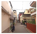
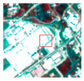
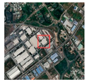
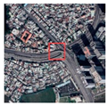
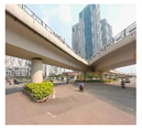
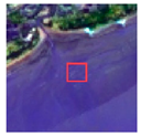
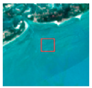
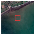
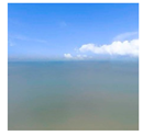
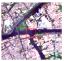
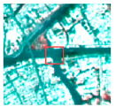
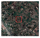
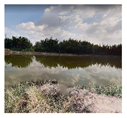
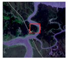
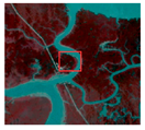
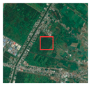
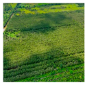
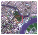
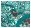
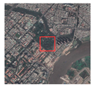
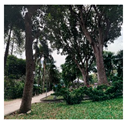
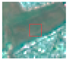
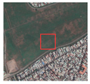
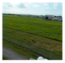
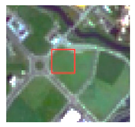
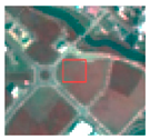
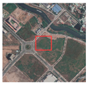
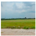
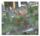
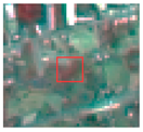
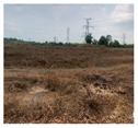
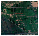
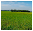
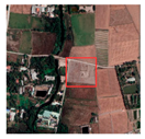
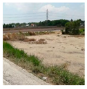
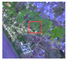
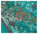
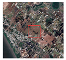
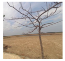
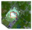
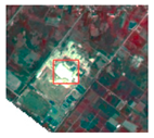
Reference data for the training and validation samples of land cover are from high-resolution Google Earth images in the same period. Meanwhile, we also looked for photos from Google Street View and Google Explore from the same period that could show land cover. These photos would verify the data reliability of Google high-resolution images and the LANDSAT8-OLI data simultaneously. A collection of land cover samples is shown in the Appendix A, corresponding to LANDSAT8-OLI data, Google high-resolution images, and field photos from the same locations during the same period. In addition, we collected the Sentinel-2 satellite 10 m land cover product and the 30-m resolution global land cover product, which was one of the methods we used to verify the scientificity and accuracy of the land cover classification results. Sentinel-2 products come from the Sentinel-2 satellite images of the European Space Agency (E.S.A.), which is produced by Esri, Microsoft, and Impact Observatory and is a composite of land use/land cover predictions for nine classes for each year from 2017 to 2021. China developed the 30 m resolution global land cover data product, and the globalland30 V2020 version was updated and released by the Ministry of Natural Resources of China. The products collected a dataset with more than 230,000 samples distributed, and the overall accuracy of the data was 85.72% while the Kappa coefficient was 0.82 [35].

2.3. Data Preprocessing

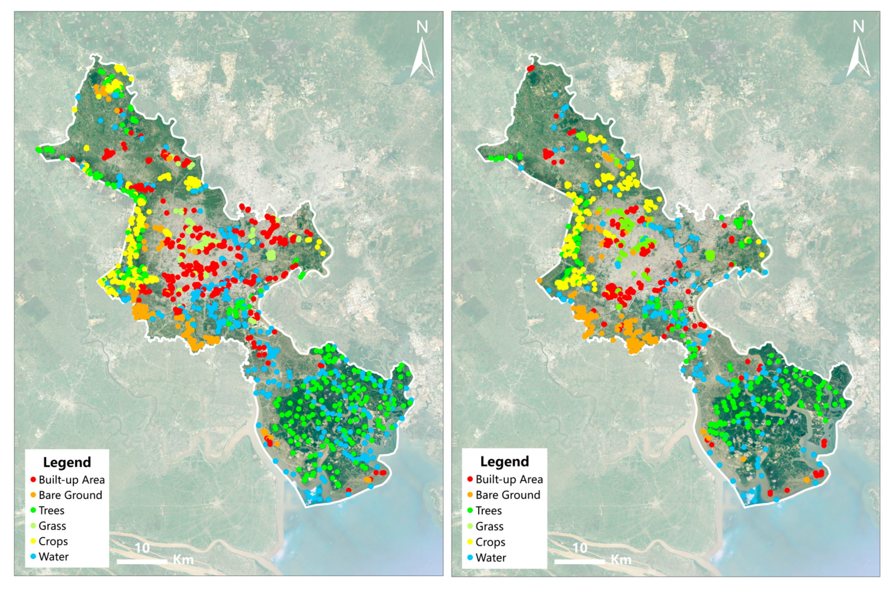
By comparing the research literature on land classification, the IGBP land classification method, and the land use patterns of Ho Chi Minh City [36,37], we divided the land cover of Ho Chi Minh City into six classifications: Built-up Area, Trees, Crops, Grass, Bare Ground, and Water. We collected 2221 land cover samples (Table 1) for the above six land cover classifications. Then, we used 60% of the collected samples for classification training and 40% for post-classification verification (Figure 2). Finally, we also performed the necessary separability judgment on the selected training and verification samples. Jeffries-Matusita and Transformed Divergence have commonly used coefficients with values between 0 and 2, with a better value closer to 2. Consider combining the two samples if values are less than 1 [38]. The Jeffries-Matusita coefficient was used in our study to determine separability. Table 2 and Table 3 show the Jeffries-Matusita coefficient of training and verification.
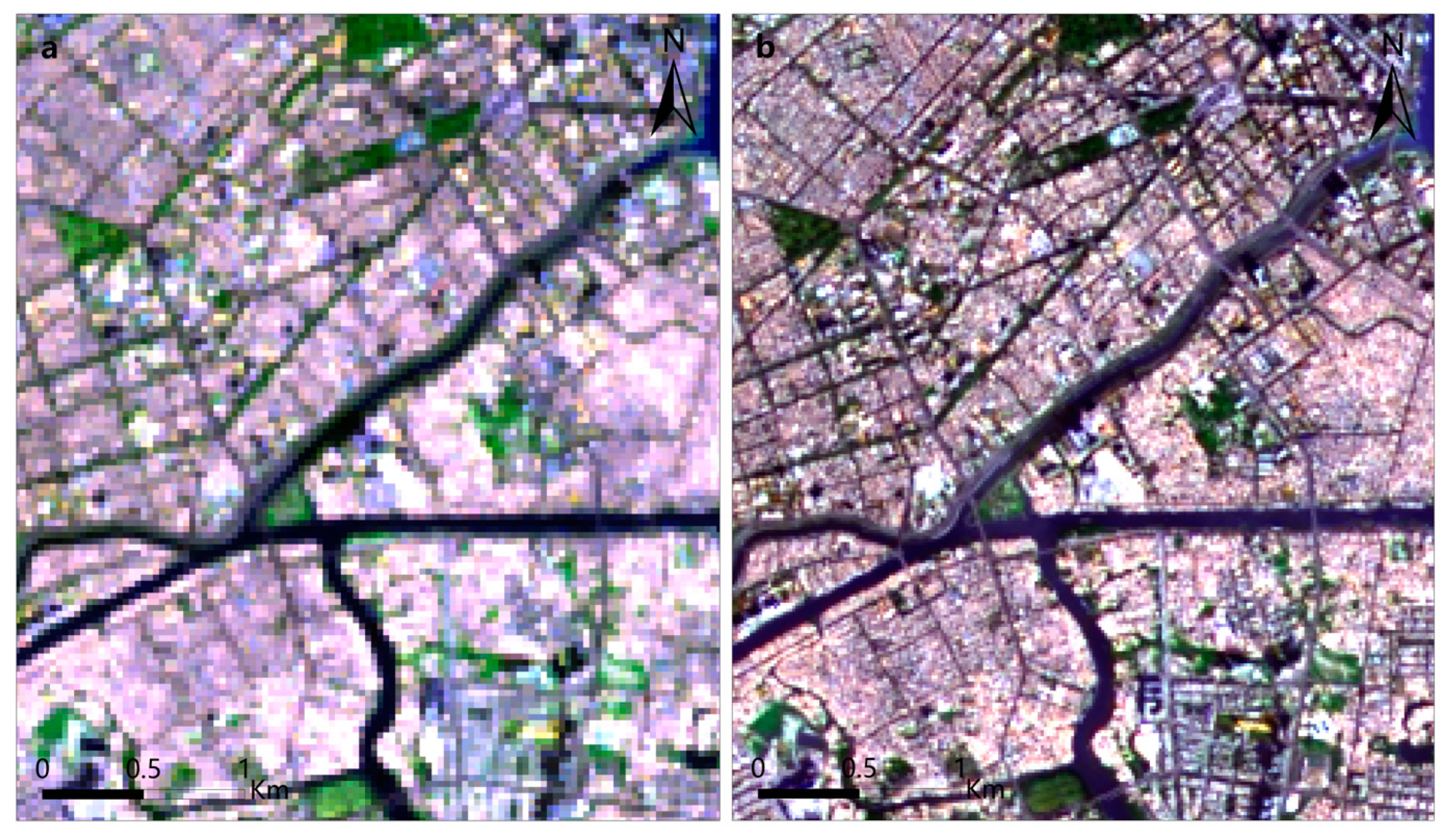
We considered the rapid development scale of the Built-up Area and the rapid expansion of construction land in Ho Chi Minh City. Moreover, suitable geographical and climatic conditions promote the lush growth of vegetation, so the Built-up Area and vegetation regions are the two main subjects of the land cover classification in Ho Chi Minh City. According to the research of ESRI and some scholars, the band combination for urban analysis using the false color band combination 764 from LANDSAT8-OLI data [39,40,41] and the band combination suitable for vegetation identification and analysis is near-infrared and visible light band combination 534 [39,42]. Then, we composited band 764 and band 543, respectively. Finally, we needed to improve the image resolution and identify the land cover situation more accurately, using the band combination 764 and band combination 543 to composite with band Pan by an Image Sharpening processing of the Gram-Schmidt algorithm [43] in ENVI5.3 software, respectively. This processing ensures the consistency of the spectral information of images before and after the composite and improves the image resolution. We obtained a better result after the Sharpening process (Figure 3b and Figure 4b) and before (Figure 3a and Figure 4a) in band combinations 764 and 543.

3. Method

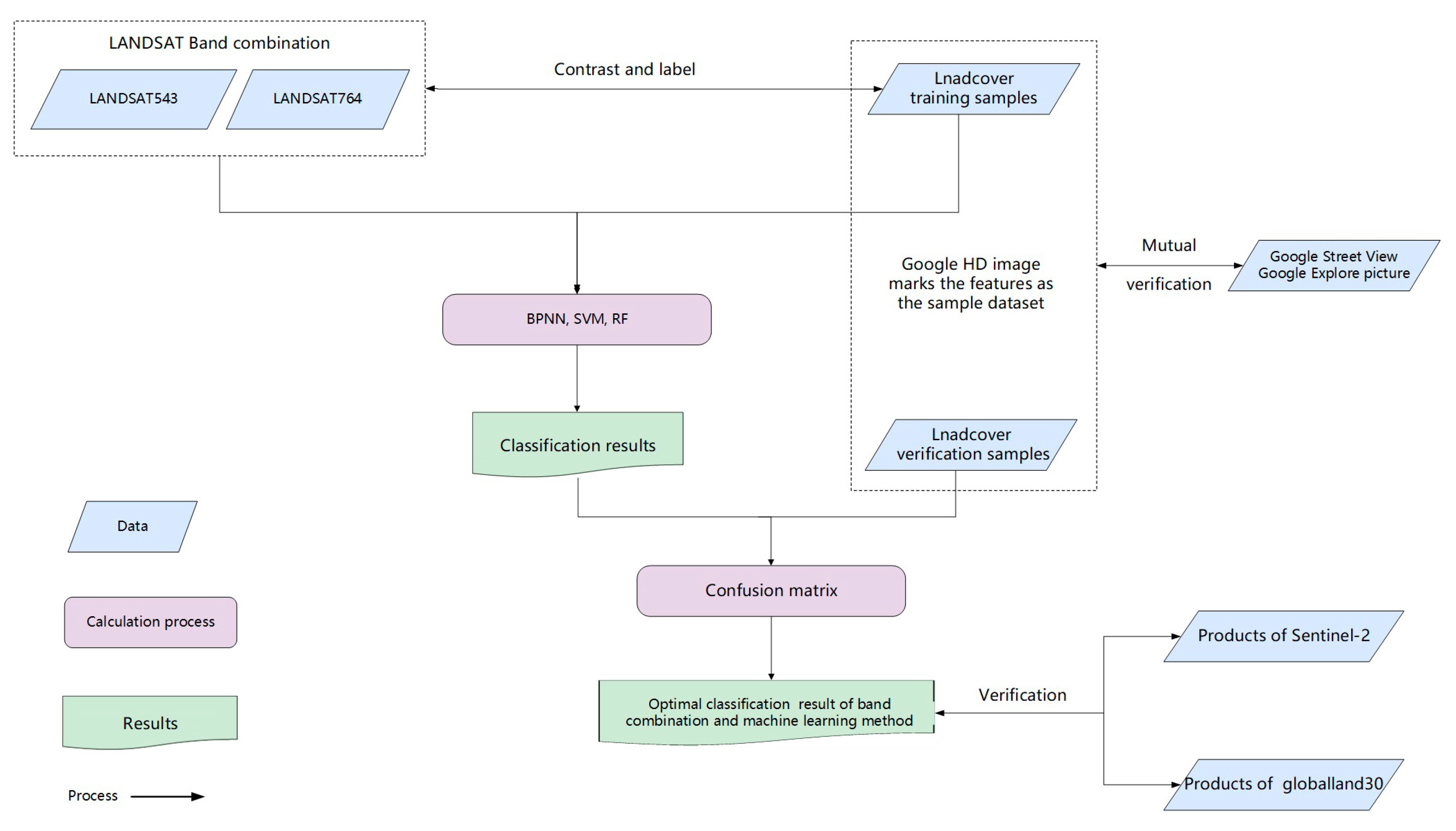
This paper proposes a method to obtain high spatial and temporal resolution urban land cover data using public satellite products. The proposed methodology employs three machine learning techniques, namely Back-Propagation Neural Network (BPNN), Support Vector Machine (SVM), and Random Forest (R.F.), to classify the land cover by analyzing two band data combinations acquired from the LANDSAT8-OLI sensor. The study further compares and validates the classification results, culminating in selecting the optimal classification scheme. The detailed flowchart is shown in Figure 5.

3.1. Back-Propagation Neural Network Algorithm (BPNN)

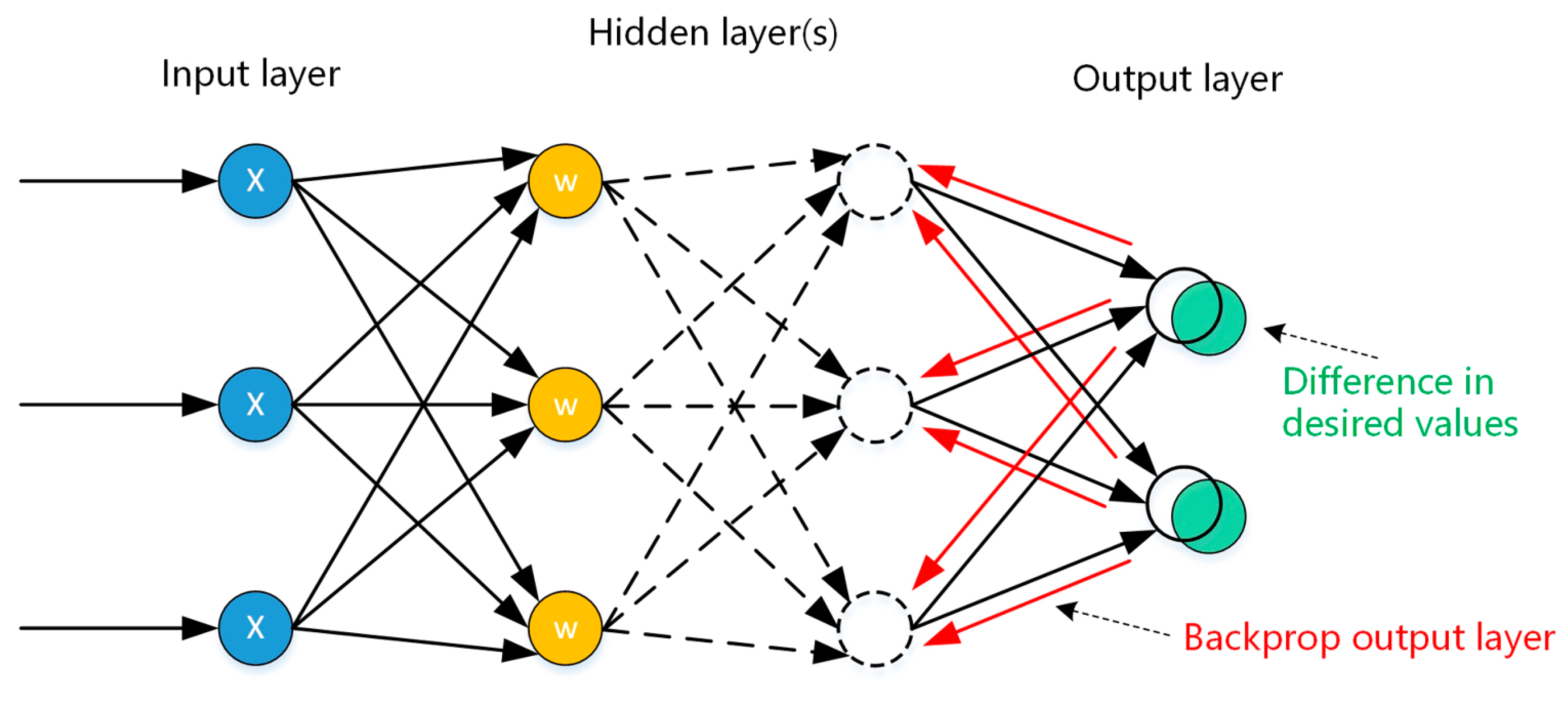
The BPNN is a widely used machine learning algorithm that effectively applies to nonlinear classification and parameter inversion in remote sensing image processing [44,45,46]. BPNN is a feed-forward multilayer neural network trained using the error back-propagation algorithm. The network has an input layer node, a hidden layer node (one layer or multiple layers), and an output layer node. The input signal should be transmitted to the hidden layer node first. After activation function processing, the output signal of the hidden layer node is transmitted to the output node, which then gives the output layer. Then, the error in the outputs is calculated. Finally, it is necessary to travel back from the output layer to the hidden layer to adjust the weights to decrease the error. The process is repeated until the desired output is achieved (Figure 6) [47]. In other words, BPNN belongs to a class of supervised learning algorithms [48].
In this study, we used the ‘S’ type function as the activation function because the S function is continuously differentiable, its classification was more accurate and reasonable than linear division, and it made the network more fault tolerant. In addition, in the back-propagation process, the iterative adjustment time of network node weights was overly lengthy, which was easy to make the training process fall into the local minimum. After the manual tuning of the hyperparameters based on experience, the final values of 0.9 and 0.1 were obtained by comparing the results of the training weights and R.M.S. thresholds over multiple attempts. We tried single-layer and multilayer networks to plan the network’s intermediate layers. By comparing the classification results, we found that the calculation results of the single-layer network were more consistent with the actual situation.

3.2. Support Vector Machine Algorithm (SVM)

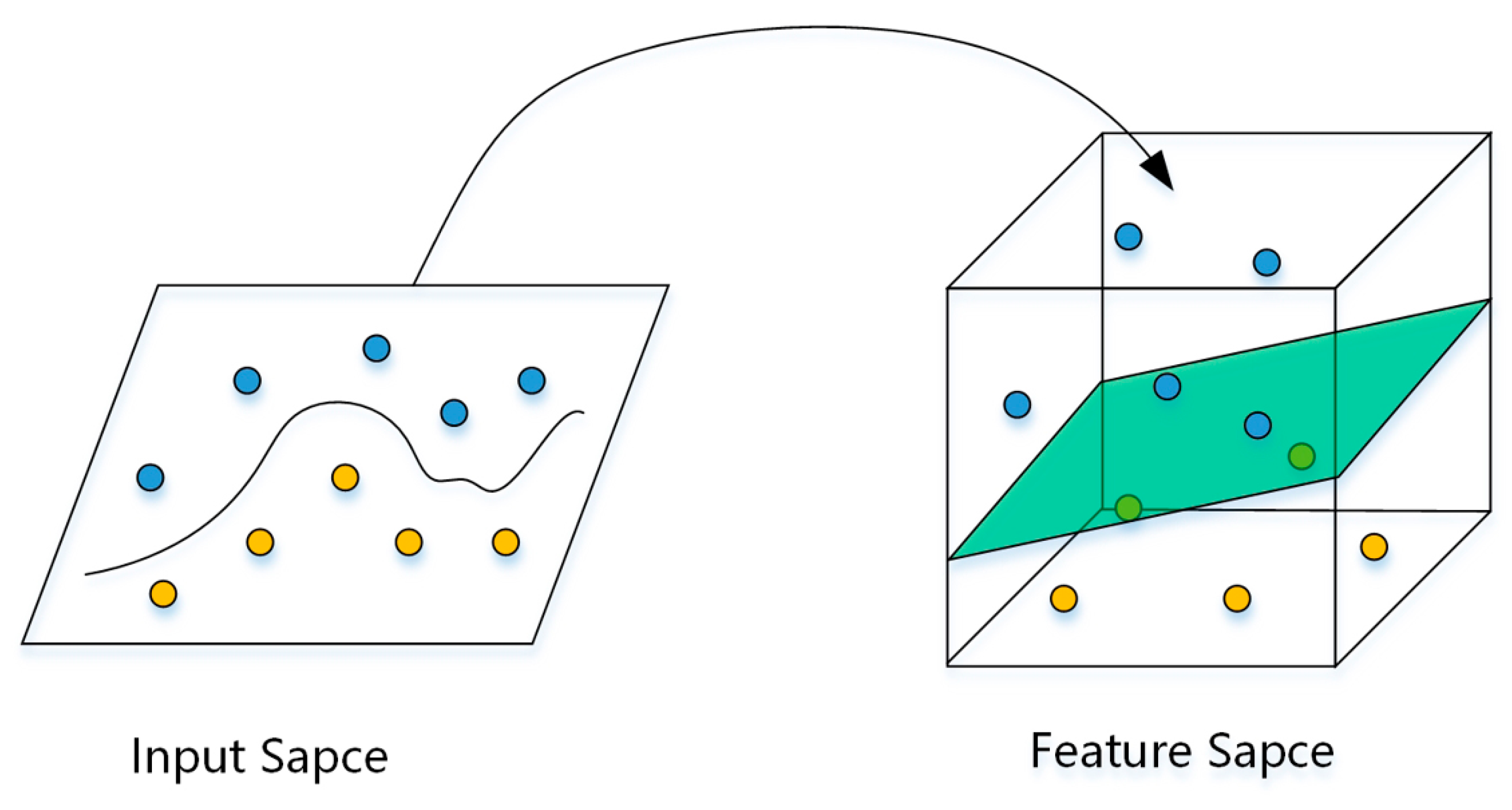
SVM is a nonparametric supervised machine learning technique initially designed to solve binary classification problems [49,50]. It separates the data with a decision surface that maximizes the margin between the data classes. It enables low-dimensional samples to be projected into high-dimensional space, yielding good classification results from complex and noisy data [51,52,53]. The flowchart of the SVM algorithm is shown in Figure 7. The decision surface is usually called the optimal hyperplane. The data samples closest to the hyperplane are called support vectors, as the critical training set elements [54]. In addition, SVM allows a certain degree of misclassification by a penalty parameter and controls the trade-off between allowing training errors and forcing rigid margins, which is particularly important for non-separable training sets. Using nonlinear kernels, we can adapt SVM to become a nonlinear classifier in remote sensing image classification applications. The most commonly used kernel functions are the radial basis function (RBF), S-type function, and polynomial function. Still, RBF is the most popular technique for land cover classification and has better accuracy than other traditional algorithms [50].
The Kernel function is a highly significant index in the classification of the SVM algorithm. In this study, we chose the RBF kernel function for classification calculation since the RBF kernel function can map a sample to a higher dimensional space, and fewer parameters need to be determined. In addition, after manually tuning the hyperparameters and comparison, we decided that the penalty and Gamma coefficients were 100.00 and 0.33, respectively.

3.3. Random Forest Algorithm (R.F.)

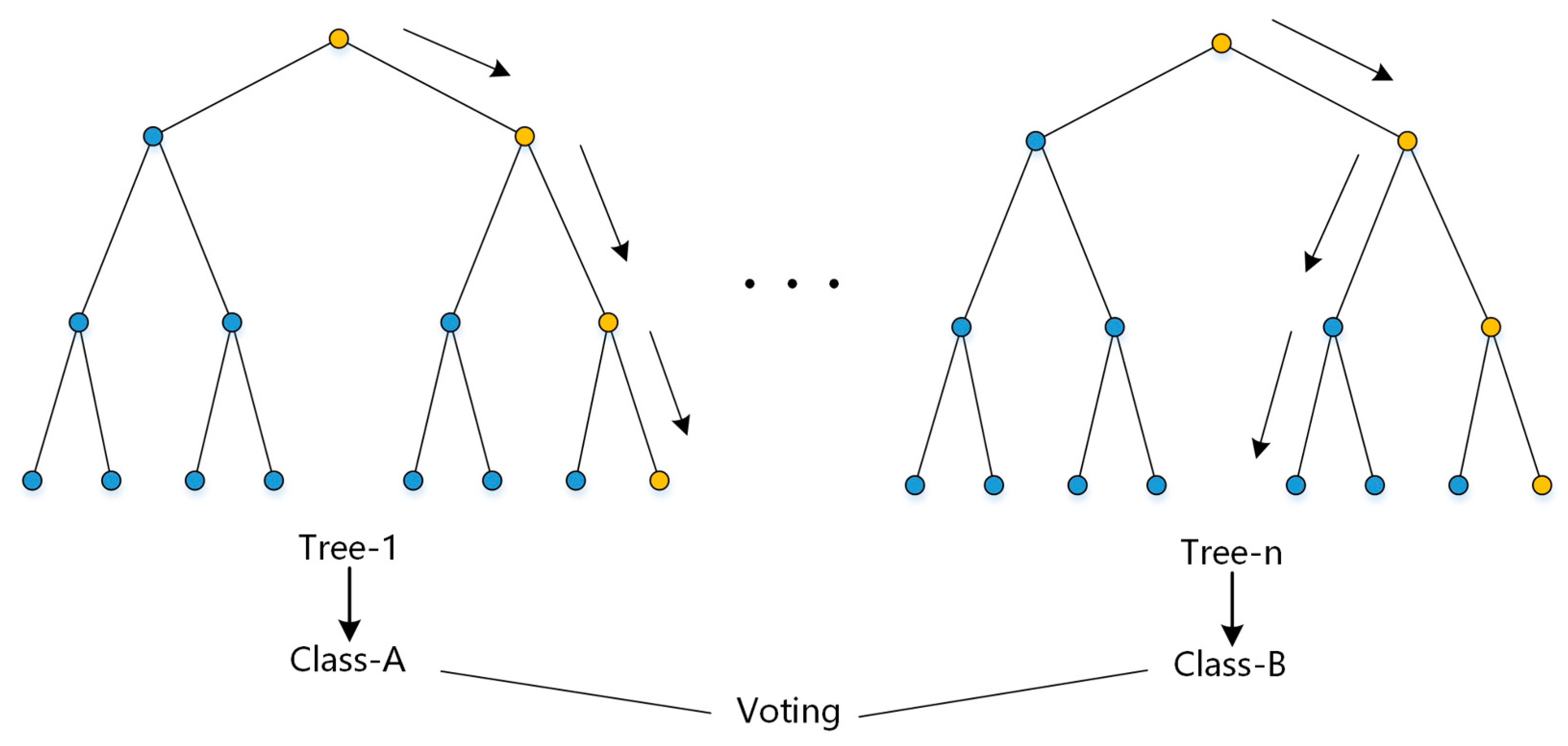
R.F. is an ensemble learning method based on a nonparametric regression algorithm proposed by Leo Breiman in 2001, which can also be regarded as a particular machine learning technique based on the iterative and random creation of decision trees. In remote sensing image data classification, Random Forest creates several decision trees randomly and splits the trees based on calculating the Gini coefficient. Then, the importance of input features according to the contribution thereof to the decision trees model is evaluated. Finally, a model based on the decision trees is created and used to classify all the pixels [55]. The flowchart of the R.F. algorithm is shown in Figure 8. Compared with traditional decision trees, it is more robust and has better generalization performance than single decision trees. Some studies have shown that using R.F. for land cover classification in remote sensing applications performs satisfactorily [56,57]. This algorithm utilizes many decision trees to provide better accuracy in image classification and land use modeling and is one of the most effective machine learning methods available [58].
In this study, we mainly tune and compare three parameters: the number of decision trees, the random feature variables, and the impurity function. If the number of decision trees is N, when N ≥ 100, the out-of-bag error of each classification tends to be stable, and there is no overfitting phenomenon in the R.F. Thus, after manually tuning the hyperparameters and comparison, we set the value N to 200. The number of random feature variables m is based on Breiman’s suggestion, and we set m (the number of random feature variables) equal to the square root of m (the total number of feature variables) for classification. In addition, we chose the Gini Coefficient as the impurity function.

3.4. Classification Accuracy Verification

Accuracy evaluation is an essential process to measure the reliability of remote sensing image classification. It compares two classified images, one of which has been classified for evaluation, and the other is the accurate reference map of the hypothesis [59]. The most commonly used method for accuracy evaluation is the confusion matrix. Different accuracy types, such as overall accuracy, user accuracy, cartographic accuracy, and the Kappa coefficient, can be calculated [60,61].

4. Results

4.1. Classification Results of the BPNN Algorithm

We used the BPNN algorithm to classify the land cover of the two band combinations. The result showed that in terms of the overall classification accuracy, band combination 764 was 99.18%, higher than band combination 543, which was 97.63%, and the Kappa coefficient was 0.987 for band combination 764, higher than 0.961 for band combination 543 (Table 4). The results of land cover accuracy of different classifications also showed that band combination 764 was better than band combination 543. In addition, it was also apparent that when comparing band combination 764 with band combination 543, the production accuracy was 92.07% and 77.24% for grassland, 66.98% and 33.02% for Bare Ground, and 97.26% and 41.92% for user accuracy. The rest of the land classification accuracy has a slight difference.
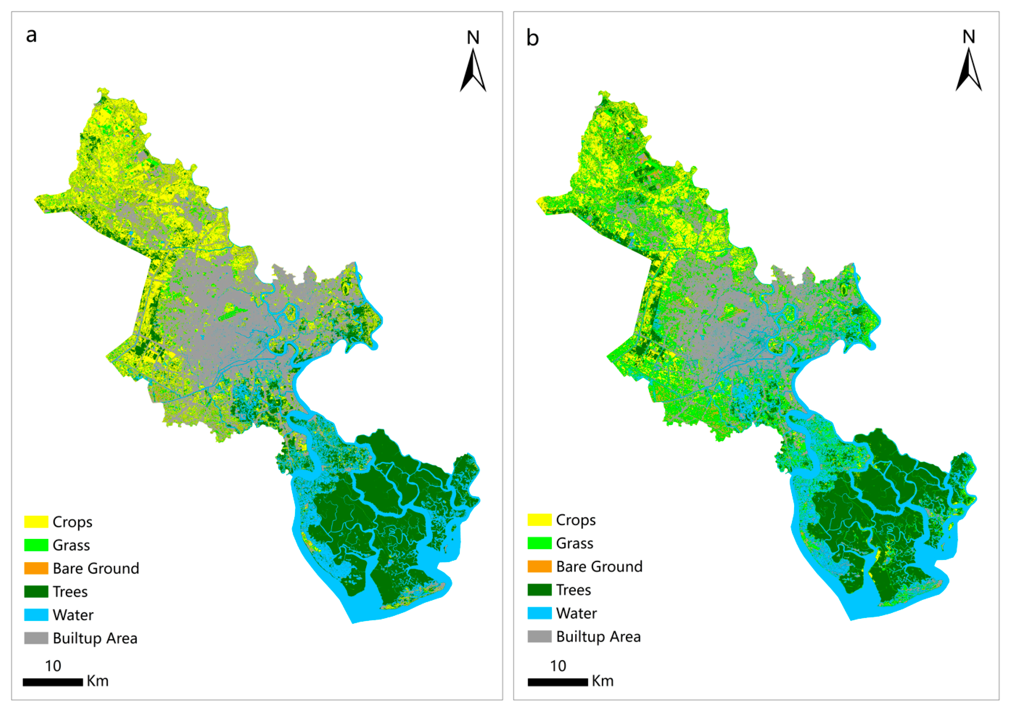
According to the results of the BPNN algorithm, the classified area of each land cover in band combination 764 (Figure 9a) was 387.66 km2 for Crops, 134.62 km2 for Grass, 44.51 km2 for Bare Ground, 512.02 km2 for Trees, 403.62 km2 for Water, and 629 km2 for Built-up Area. The classified area of each land cover in band combination 543 (Figure 9b) was 257.32 km2 for Crops, 404.45 km2 for Grass, 81.49 km2 for Bare Ground, 450.26 km2 for Trees, 443.42 km2 for Water, and 474.49 km2 for Built-up Area.

4.2. Classification Results of the SVM Algorithm

The classification results’ accuracy of the two band combinations by the SVM algorithm is shown in Table 5. Regarding the overall classification accuracy, band combination 764 is 99.38%, higher than band combination 543’s 99.11%, and band combination 764’s Kappa coefficient was 0.990, which was higher than band combination 543’s 0.985. There was a minor difference in the accuracy of the classification results of the two band combinations in different land classifications. Still, band combination 764’s classification results were better than those of band combination 543.
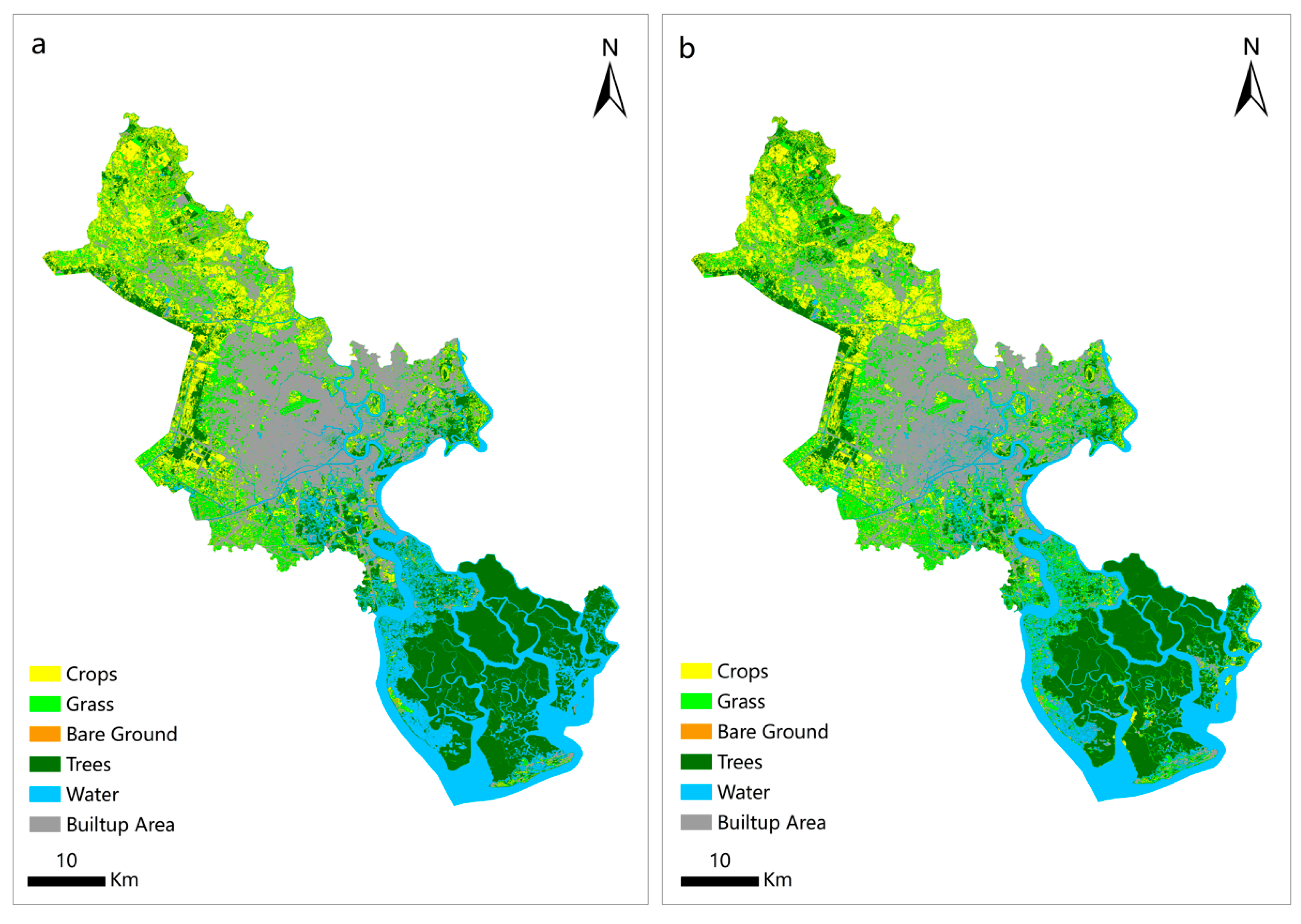
According to the classification result of the SVM algorithm, the classified area of each land cover in band combination 764 (Figure 10a) was 304.04 km2 for Crops, 262.07 km2 for Grass, 27.55 km2 for Bare Ground, 545.53 km2 for Trees, 414.31 km2 for Water, and 557.95 km2 for Built-up Area. The classified area of each land cover in band combination 543 (Figure 10b) was 316.78 km2 for Crops, 333.52 km2 for Grass, 9.98 km2 for Bare Ground, 535.17 km2 for Trees, 350.16 km2 for Water, and 565.83 km2 for Built-up Area.

4.3. Classification Results of the R.F. Algorithm

The accuracy of classification results based on the R.F. algorithm is shown in Table 6. Regarding overall classification accuracy, band combination 764 was 99.41%, higher than band combination 543, which was 99.17%, and the Kappa coefficient was also 0.990 for band combination 764, higher than 0.986 for band combination 543. In all the land cover classification results, the accuracy of the two band combinations was not significantly different, but the 764 band combination was superior to the 543 band combination.
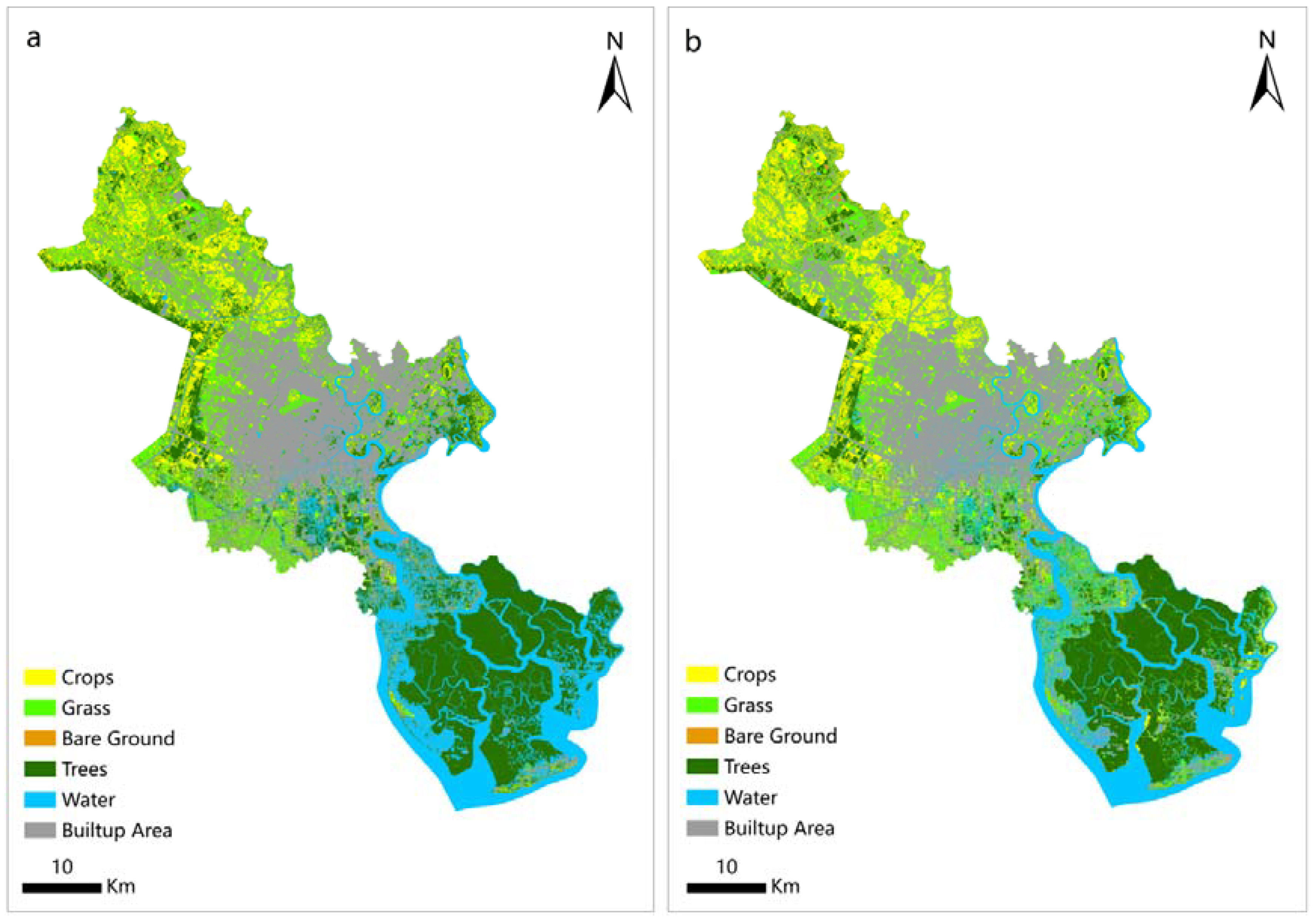
According to the classification result of the R.F. algorithm, the classified area of each land cover in band combination 764 (Figure 11a) was 221.74 km2 for Crops, 299.59 km2 for Grass, 35.98 km2 for Bare Ground, 591.21 km2 for Trees, 408.62 km2 for Water, and 554.29 km2 for Built-up Area. The classified area of each land cover in band combination 543 (Figure 11b) was 280.63 km2 for Crops, 380.95 km2 for Grass, 8.97 km2 for Bare Ground, 504.97 km2 for Trees, 330.50 km2 for Water, and 605.39 km2 for Built-up Area.

4.4. Results of Comparison with Different Land Cover Classification Products

The above classification results showed that the accuracy and Kappa coefficient of the classification results based on band combination 764 and the R.F. algorithm are the best. To verify the authenticity and accuracy of the land cover classification, we compared the classification results with other authoritative land cover classification products. We introduced the land cover classification product of Sentinel-2 satellite Ho Chi Minh City with 10 m spatial resolution and the land cover classification product of globalland30 with 30 m spatial resolution, both in 2020, and then converted the land cover type of the two products into the land cover type of our study. We compared the land cover area between the classification result of band combination 764 and the R.F. algorithm with the Sentinel-2 and Globalland30 data products, as shown in Table 7.
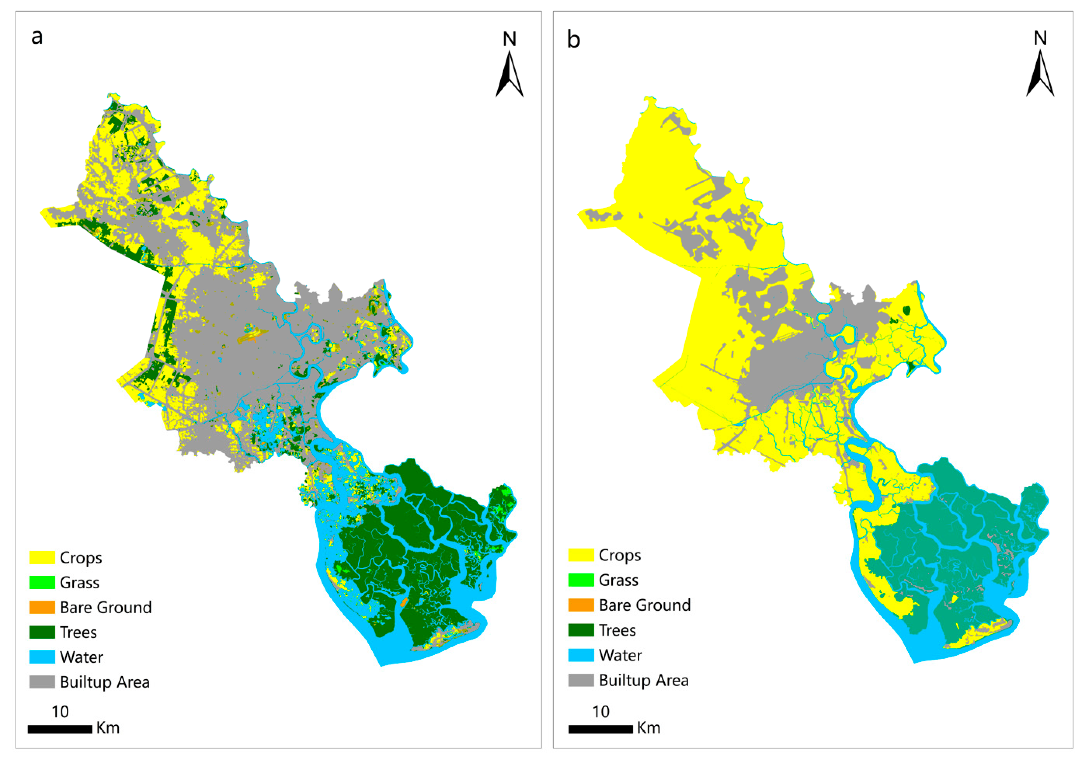
Since different data and methods are used for land cover classification, different results for land cover classification show significant spatial differences. This is mainly reflected in how the Sentinel-2 product was more sensitive to the inversion of Built-up Area, which was distributed in most of the central and northern parts of Ho Chi Minh City (Figure 12a). However, the globalland30 product focuses more on reflecting Crops. In contrast, the Built-up Area was distributed in the central part of Ho Chi Minh City, and Trees and Water were in the south. The rest were classified as Crops (Figure 12b). Our classification results showed that the Built-up Area was mainly distributed in the center of Ho Chi Minh City. In contrast, Crops and Grass were distributed primarily in the northern, mid, and western regions in a contiguous distribution pattern. Trees (mostly mangroves) were mainly distributed in the south.

5. Discussion

5.1. Authenticity Comparison of Land Cover Classification Results for Different Band Combinations

Based on the LANDSAT8-OLI image data, different band combinations show various land cover recognition advantages [39]. Band combination 764 contains shortwave infrared bands, which have better effects than bands with a shorter wavelength, making distinguishing between Built-up Areas and vegetation easier. Band combination 543 is a standard false color combination (C.I.R.) used for vegetation-related monitoring. This band combination, in which the vegetation appears red, is commonly used to monitor vegetation, crops, and wetlands. On the other hand, Ho Chi Minh City’s land cover has a significant apparent spatial distribution of the Built-up Area and vegetation (Trees dominate the south, the Built-up Area dominates the middle, and the north is dominated by vegetation, such as Crops and Trees). Therefore, studying these two band combinations is of interest for practical applications.
The results for land cover classification using two band combinations and three machine learning algorithms showed that the R.F. classification algorithm was the best. Still, the two band combinations have slightly different results for land cover classification. Short wave infrared (SWIR) was sensitive to the reflection of Bare Ground, so in the classification result of band combination 764, the Area of Bare Ground was larger than band combination 543. For the vegetation identification and classification in Ho Chi Minh City, band combination 543 had an extremely strong reflectance of vegetation in the mid-near infrared spectral channel (0.85–0.88μm), so this band combination can monitor vegetation effectively. As a result, the vegetation range of band combination 543 was more significant than that of band combination 764. In addition, different types of vegetation and different growth states of vegetation present an inconsistent reflection of near-infrared waves, which can easily lead to misclassification [62,63]. Although machine learning algorithms and large numbers of samples can be used to classify land cover as accurately as possible, there can still be misclassifications. From this, we need to identify the most suitable band combination of land cover classification in Ho Chi Minh City by comparing the classification results with the actual features.
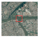
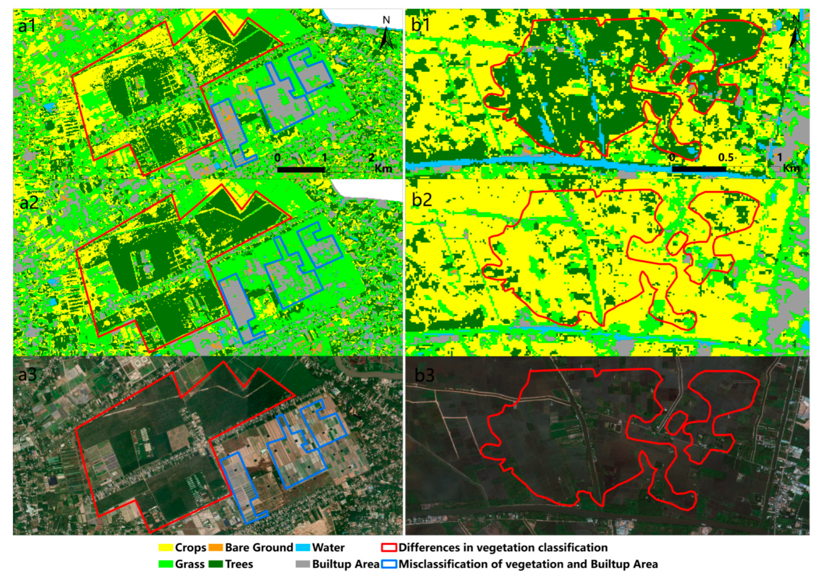
We compared the classification results of two band combinations with actual features. Band combination 543 was more reasonable in vegetation type recognition (Figure 13(a2,b2)). However, some artificial features were easily confused with the natural land cover, leading to misclassification. For example, the plastic film of the artificial planting greenhouse was identified as Built-up Area by band combination 764 and band combination 543 (Figure 13(a1,a2)). Similar misclassifications could occur in plastic membranes at the bottom of dry artificial salt fields, part of the dry land during the fallow period, and solar power equipment on the Grass or Water, among others. The result of band combination 764 misclassified minor areas of paddy fields that had not yet grown seedlings as Trees in east Ho Chi Minh City (Figure 13(b1)). In addition, some Crops or short trees on farmland would also be misclassified as Grass (Figure 13(b2)). For the above cases, the expressions for some of the different land cover spectra and textures would be rather similar in the composite band combinations with a resolution of 10m to 30m, which may be the reason for misclassification. Moreover, given the complex situation of local land cover and the rapid shift of the time series, we believe that visual interpretation adjustment after classification is a more appropriate treatment when the classification type of land cover is not complicated.
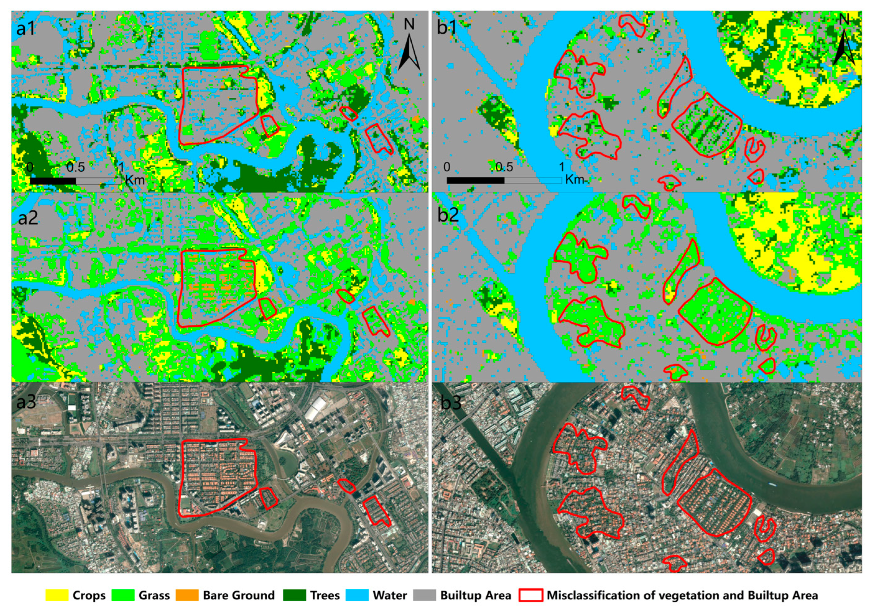
The land in the Built-up Area has a strong reflection of shortwave infrared but a low reflection of the near-infrared band (Nir) [64]. Band 7 and band 6 are the bands of shortwave infrared in band combination 764. Compared with the band combination, which has a shorter wavelength, the effect of band combination 764 was better, and the Built-up Area, such as the house in the residential area, could be judged more accurately (Figure 14(a1,b1)). Band combination 543, on the other hand, focuses more on the green plants in residential areas, such as seedlings, flowers, and other vegetation (Figure 14(a2,b2)).
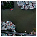
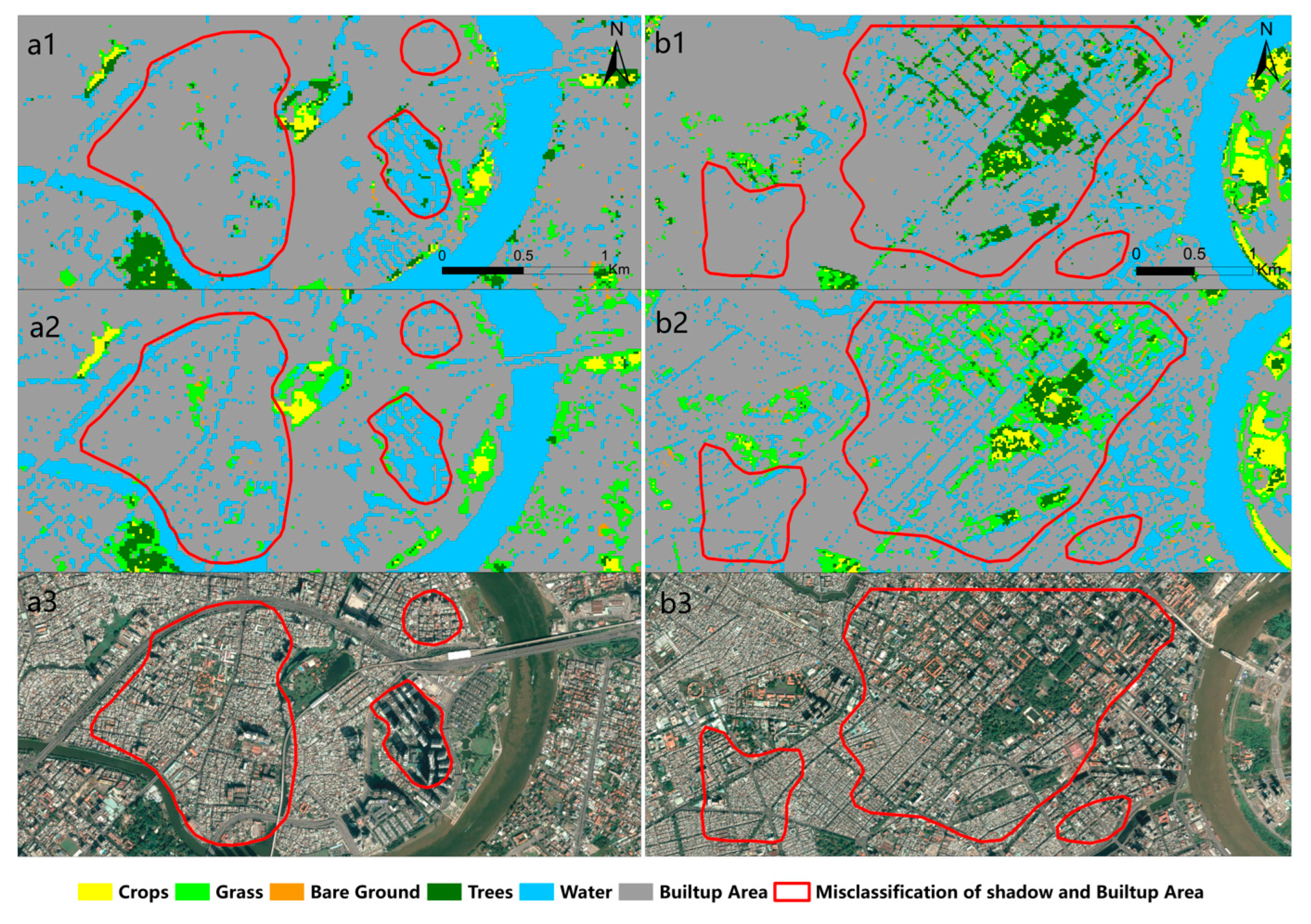
Because of the strong reflection of Water in the shortwave infrared (SWIR) range of 1.57–1.65μm, band combination 764 is more sensitive to Water than band combination 543, which also explains why the classification result of Water in band combination 764 was about 80 km2 more than band combination 543. However, band combination 764 and band combination 543 would be confused by the shadow of buildings and tall trees during the identification of Water (Figure 14), which may lead to misclassification. Numerous scholars have conducted studies on water extraction from LANDSAT8-OLI data. Most of the studies have considered the influence of mountain and cloud shadows on the extraction of water scope, such as the water index method based on a large number of sample data [65], the unsupervised classification method based on a multi-spectral operation [66], and the water extraction method based on multilayer neural network [65]. These studies are all based on a national or regional scale or in the natural environment of a small watershed, where it is relatively easy to identify significant areas of shadow. However, for the continuous shadow of buildings in the city and the dappled shadows of the tall trees on the streets, the misclassification caused by them with the urban internal water system is worth further research. For this problem, some scholars believe that the decision tree could identify the shadow of obstacles in a limited range by combining the vegetation and water indexes to distinguish the shadow from the water body and obtain excellent classification results [67].
Our study found that most of the misclassifications of shadows and Water were located in the central area of Ho Chi Minh City. Because there were numerous rivers and ditches in the city’s urban area, the shadows of high buildings and tall trees on both sides of the urban roads reflected similar spectra and textures to the Water in river ditches of the central area (the shadows extended along the road). As a result, the shadows of buildings and tall trees on either side of the road in the central city were confused with Water and caused misclassification. Comparing the classification results of the two band combinations, band combination 764 had fewer misclassification results and was closer to the actual situation (Figure 15(a1,b1)). Band combination 543, on the other hand, classified the shadow more as Water. However, band combination 543 could accurately identify the landscape vegetation of the road (Figure 15(a2,b2)). For this misclassification of shadow and Water, we could process it through visual interpretation after classification. Alternatively, multi-spectral classification algorithms based on scene range and machine learning with a large number of samples might also be a path to solve the problem.

5.2. Applicability Comparison of Land Cover Classification Results of Different Machine Learning Algorithms

Based on band combination 764, we compared the classification results of the three machine learning algorithms. We found that the R.F. algorithm gave the best classification accuracy, overall accuracy, and Kappa coefficient. Therefore, we took the result area of R.F. classification as the benchmark and compared the result of the other two algorithms (Table 8) to discuss the differences in the classification results of each algorithm. Finally, we tried to find a more suitable algorithm for land cover classification in Ho Chi Minh City.
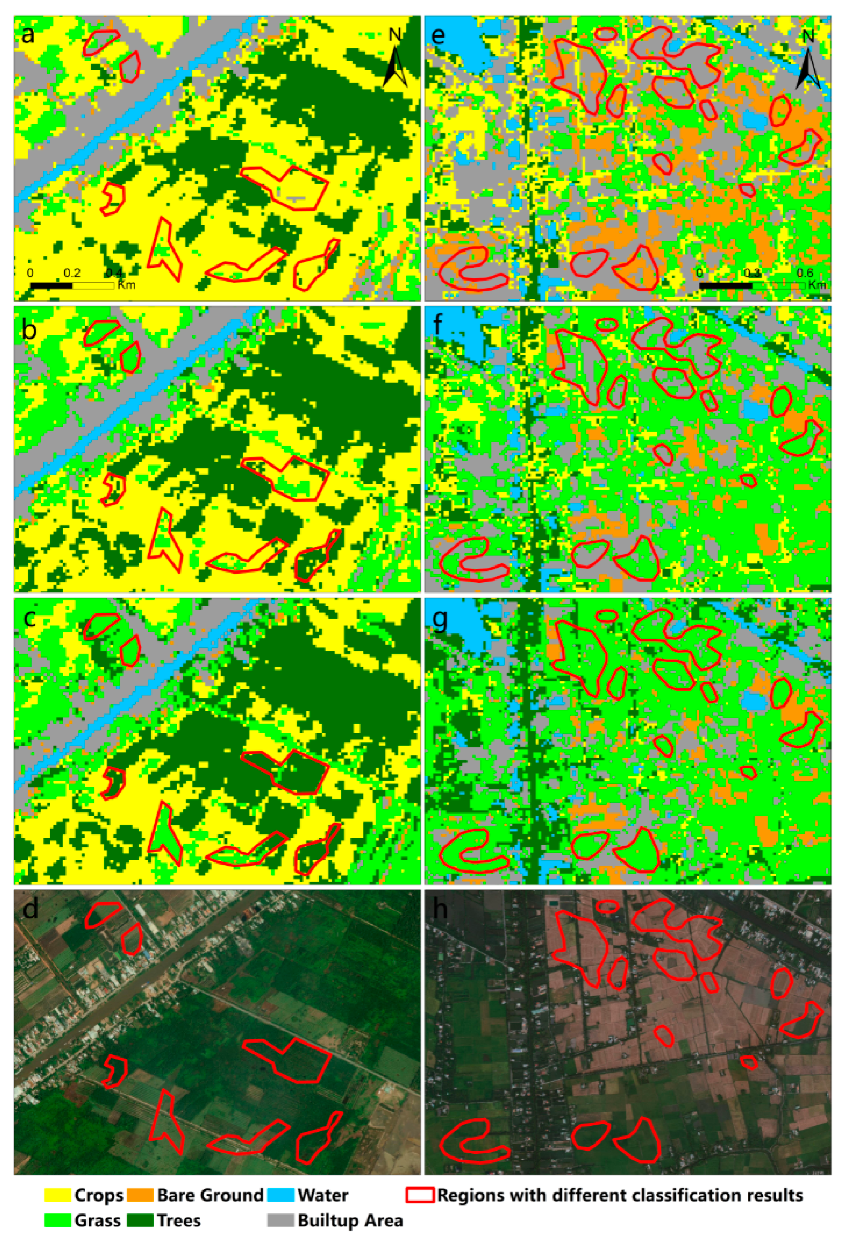
By comparison, we found that Crops, Trees, and Grass areas differed significantly in the three algorithms’ classification results. Then, based on the classification results of band combination 764 and the three machine learning algorithms, we carefully analyzed the areas in the east and southeast of Ho Chi Minh City where there were more Crops, Grass, and Trees intersecting each other (Figure 16). In the east of Ho Chi Minh City, which mixed vegetation planting regions of Crops and Trees (nursery), we found three algorithms misclassified. The results of the BPNN algorithm misclassified some Trees as Crops (Figure 16a). The results of the SVM algorithm misclassified some Trees as Grass and Crops (Figure 16b). The results of the R.F. algorithm classified those land covers as Trees mostly (Figure 16c), but this was consistent with the actual situation basically (Figure 16d). Thus, we think the best order of application for the three algorithms was R.F., SVM, and BPNN. In the southeast of Ho Chi Minh City, the seasonal rotation region, we found that all three algorithms classified part of Crops land without planting as Grass. The classification results of the BPNN algorithm (Figure 16e) and SVM algorithm (Figure 16f) organized pieces of Crops land without planting as Built-up Area and Bare Ground. However, the classification result of the R.F. algorithm classified them as Grass in most cases (Figure 16g). We commonly classify planting areas without crops as Bare Ground. Comparing it with the actual ground features (Figure 16h), we found that the closest degree of the three machine learning classification algorithms to the actual ground features was the BPNN, SVM, and R.F. algorithms. Different classification results may be due to different algorithms and deserve further exploration. By comparing the classification results of the three machine learning algorithms, we found that the R.F. algorithm gave the best classification results in most cases, followed by the SVM algorithm and then the BPNN algorithm.

5.3. Comparison of Classification Results with Other Land Cover Classification Products

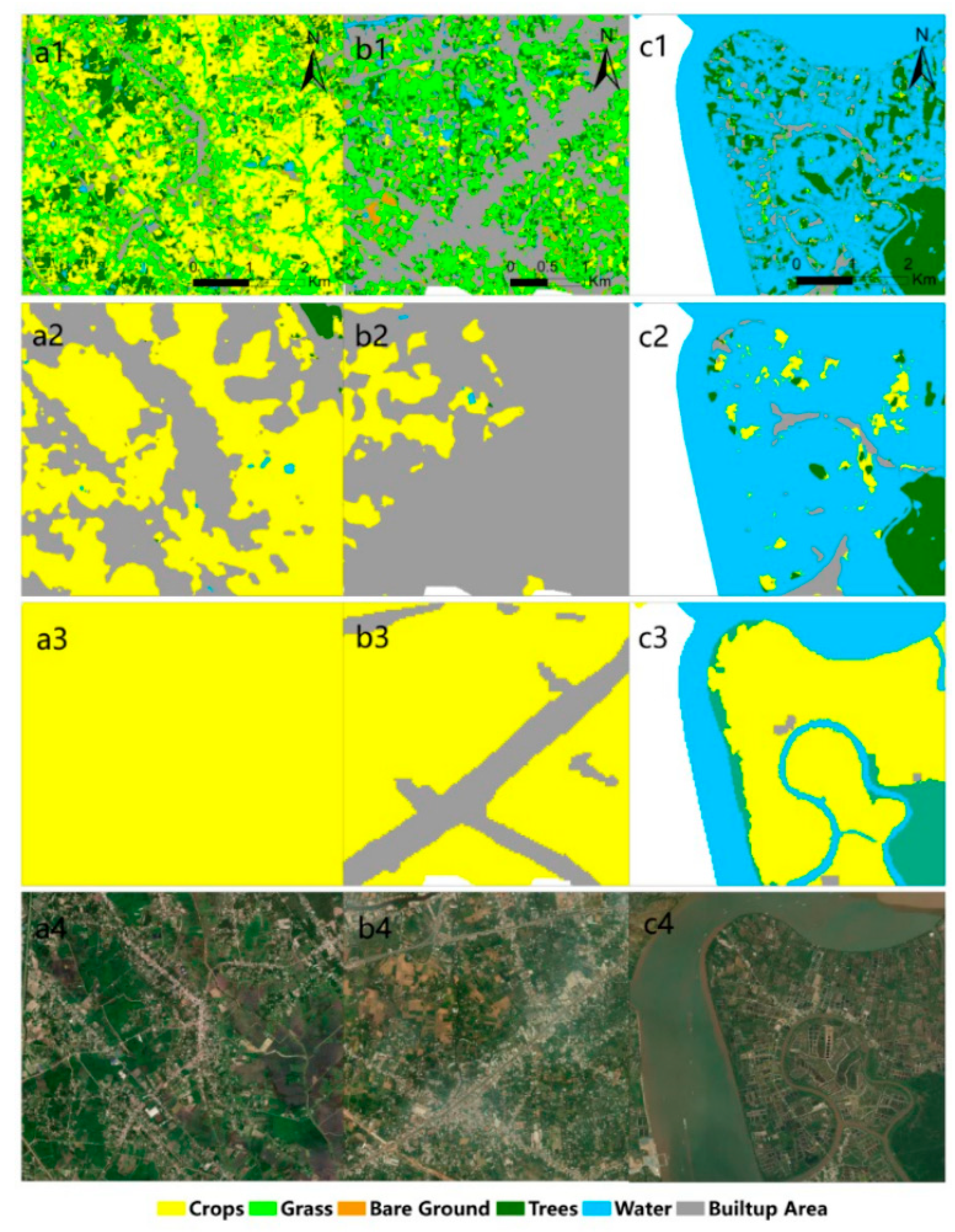
This study’s land cover classification in Ho Chi Minh City was conducted based on two band combinations and three machine learning algorithms, which obtained excellent classification accuracy and the Kappa coefficient. Based on the classification results, we found that a minor part of vegetation was misclassified in the verification process with actual ground features. The high spatial aggregation of some land cover sample data of the same type might cause misclassification. Considering this issue, we also introduced the currently widely used land cover classification products Sentinel-2 and globalland30 and compared them with our classification results. Sentinel-2 and globalland30 are global-scale land cover classification results. Both of the products mentioned above were crude and inconsistent with actuality in city-level features, especially the classification results for local details (Figure 17). According to the results of Sentinel-2, some Crops were directly classified as Water in the south of Ho Chi Minh City (Figure 17(c3)). In addition, some Crops and Grass were even classified as Built-up Area in the southeast and north of Ho Chi Minh City (Figure 17(a2,b2)). As a result of globalland30, some Bare Ground, Grass, Trees, and Built-up Areas were classified as Crops in the east and north of Ho Chi Minh City (Figure 17(a3,b3)). The above two products are global-scale products, so the details of land classification within the city level cannot be considered in acquiring classification samples, which may be one reason for misclassification. Moreover, the land cover classification of different data products is inconsistent, which may cause misclassification. Regardless of the reasons, there is a significant gap between the land cover classification products of Sentinel-2 and globalland30 and the actual land cover features at the city level. Therefore, we believe these two products need further processing before they can be applied to city-level land cover classification.
For land cover classification in a specific city, the best approach is to train on a large amount of measured data and compute the land cover classification using machine learning algorithms to obtain the results. Many training samples based on measurement can adapt to the city’s long-term land cover classification because they carry the city characters. In addition, training samples can be updated according to the actual situation to adapt to the city’s land cover change, which ensures the reliability and timeliness of land cover classification.
Compared with similar urban and regional land cover classification studies in the ASEAN region [20,22,23,24] or other data products [34,35], our research can obtain classification schemes to achieve monthly and quarterly land cover renewal. Regarding spatial and temporal resolution, it can undoubtedly meet the requirements of land cover change monitoring for the rapid development of megacities in ASEAN. In addition, machine learning-based classification schemes can continuously accumulate samples of classification data during follow-up monitoring and land cover field validation, which can improve classification accuracy. At the same time, this accumulation process can also accommodate the diversity of land cover changes during urban development. Finally, based on the continuous accumulation of a sample database, it can meet urban development’s low-cost and flexible application to land cover monitoring.

6. Conclusions

Our study aimed to classify Ho Chi Minh City’s land cover classification using two band combinations of LANDSAT8-OLI data and three machine learning algorithms. We then compared the classification results with actual ground features and authoritative products to improve the rationality and practicability of land cover classification. The following conclusions were obtained through the study. (1) The effect of using band combination 764 and the R.F. algorithm for land cover classification in Ho Chi Minh City was the most appropriate. (2) There would still be misclassification in the result of land cover classification by machine learning algorithms. Due to the complexity of human activities, we believe that even an intelligent artificial intelligence algorithm would cause misclassification and thus fail to meet the requirements for land cover classification at the production level. Therefore, our recommended approach for handling the minor part of misclassification after machine learning classification was visual interpretation processing through field surveys. Finally, the reliability of the sample data set is gradually improved through empirical accumulation. (3) For global land cover data products with high spatial resolution, there are many misclassification cases in land cover classification at the city level. Further processing is needed before application at the city level. (4) It used public satellite products, reliable sample data, suitable machine learning algorithms, and human intervention to correct misclassifications, which can achieve a relatively reliable city-level land cover classification method. Meanwhile, regarding timeliness and economic cost, it can also satisfy the effective supervision of urban land in developing countries.

Author Contributions

All authors contributed extensively to the study presented in this manuscript. C.H. (Chaoqing Huang), C.H. (Chao He) and S.H.: Conceptualization, Methodology, Data curation, Visualization, Writing—original draft and editing, and Supervision. Q.W. and M.N.: Data curation, Investigation, and Validation. All authors have read and agreed to the published version of the manuscript.

Funding

This research received no external funding.

Data Availability Statement

Data will be made available upon request.

Conflicts of Interest

The authors declare that they have no known competing financial interests or personal relationships that could have appeared to influence the work reported in this paper.

Appendix A

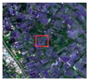
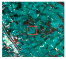
Table A1. Collection of land cover samples in Ho Chi Minh City.
Ground FeaturesBand Combination 764Band Combination 543PositionStreet ViewCoordinates
(Latitude, Longitude)
Built-up AreaSustainability 15 06798 i001Sustainability 15 06798 i002Sustainability 15 06798 i003Sustainability 15 06798 i00410.792473, 106.667262
Sustainability 15 06798 i005Sustainability 15 06798 i006Sustainability 15 06798 i007Sustainability 15 06798 i00810.829346, 106.799270
Sustainability 15 06798 i009Sustainability 15 06798 i010Sustainability 15 06798 i011Sustainability 15 06798 i01210.789532, 106.716194
WaterSustainability 15 06798 i013Sustainability 15 06798 i014Sustainability 15 06798 i015Sustainability 15 06798 i01610.381218, 106.943331
Sustainability 15 06798 i017Sustainability 15 06798 i018Sustainability 15 06798 i019Sustainability 15 06798 i02010.752191, 106.690308
Sustainability 15 06798 i021Sustainability 15 06798 i022Sustainability 15 06798 i023Sustainability 15 06798 i02410.645197, 106.795583
TreesSustainability 15 06798 i025Sustainability 15 06798 i026Sustainability 15 06798 i027Sustainability 15 06798 i02810.504798, 106.868985
Sustainability 15 06798 i029Sustainability 15 06798 i030Sustainability 15 06798 i031Sustainability 15 06798 i03210.882809, 106.543391
Sustainability 15 06798 i033Sustainability 15 06798 i034Sustainability 15 06798 i035Sustainability 15 06798 i03610.789399, 106.706238
GrassSustainability 15 06798 i037Sustainability 15 06798 i038Sustainability 15 06798 i039Sustainability 15 06798 i04010.823842, 106.676173
Sustainability 15 06798 i041Sustainability 15 06798 i042Sustainability 15 06798 i043Sustainability 15 06798 i04410.839985, 106.812435
Sustainability 15 06798 i045Sustainability 15 06798 i046Sustainability 15 06798 i047Sustainability 15 06798 i04810.684276, 106.554909
CropsSustainability 15 06798 i049Sustainability 15 06798 i050Sustainability 15 06798 i051Sustainability 15 06798 i05210.749396, 106.498723
Sustainability 15 06798 i053Sustainability 15 06798 i054Sustainability 15 06798 i055Sustainability 15 06798 i05611.033259, 106.472815
Sustainability 15 06798 i057Sustainability 15 06798 i058Sustainability 15 06798 i059Sustainability 15 06798 i06010.929771, 106.572075
Bare
Ground
Sustainability 15 06798 i061Sustainability 15 06798 i062Sustainability 15 06798 i063Sustainability 15 06798 i06410.696127, 106.559957
Sustainability 15 06798 i065Sustainability 15 06798 i066Sustainability 15 06798 i067Sustainability 15 06798 i06810.465401, 106.777864
Sustainability 15 06798 i069Sustainability 15 06798 i070Sustainability 15 06798 i071Sustainability 15 06798 i07210.964576, 106.439237

References

  1. Gong, P.; Wang, J.; Yu, L.; Zhao, Y.C.; Zhao, Y.Y.; Liang, L.; Niu, Z.G.; Huang, X.M.; Fu, H.H.; Liu, S.; et al. Finer resolution observation and monitoring of global land cover: First mapping results with Landsat TM and ETM+ data. Int. J. Remote Sens. 2013, 34, 2607–2654. [Google Scholar] [CrossRef]
  2. Yang, J.; Gong, P.; Fu, R.; Zhang, M.H.; Chen, J.M.; Liang, S.L.; Xu, B.; Shi, J.C.; Dickinson, R. The role of satellite remote sensing in climate change studies. Nat. Clim. Chang. 2013, 3, 875–883. [Google Scholar] [CrossRef]
  3. Sun, C.; Koenig, H.J.; Uthes, S.; Chen, C.; Li, P.; Hemminger, K. Protection effect of overwintering water bird habitat and defining the conservation priority area in Poyang Lake wetland, China. Environ. Res. Lett. 2020, 15, 125013. [Google Scholar] [CrossRef]
  4. Chen, J.; Chen, J.; Liao, A.P.; Cao, X.; Chen, L.J.; Chen, X.H.; He, C.Y.; Han, G.; Peng, S.; Lu, M.; et al. Global land cover mapping at 30 m resolution: A POK-based operational approach. ISPRS J. Photogramm. Remote Sens. 2015, 103, 7–27. [Google Scholar] [CrossRef]
  5. Yu, L.; Wang, J.; Li, X.C.; Li, C.C.; Zhao, Y.Y.; Gong, P. A multi-resolution global land cover dataset through multisource data aggregation. Sci. China Earth. Sci. 2014, 57, 2317–2329. [Google Scholar] [CrossRef]
  6. Hashem, N.; Balakrishnan, P. Change analysis of land use/land cover and modelling urban growth in Greater Doha, Qatar. Ann. GIS 2015, 21, 233–247. [Google Scholar] [CrossRef]
  7. Zhao, Y.Y.; Feng, D.L.; Yu, L.; Wang, X.Y.; Chen, Y.L.; Bai, Y.Q.; Hernández, H.J.; Galleguillos, M.; Estades, C.; Biging, G.S.; et al. Detailed dynamic land cover mapping of Chile: Accuracy improvement by integrating multi-temporal data. Remote Sens. Environ. 2016, 183, 170–185. [Google Scholar] [CrossRef]
  8. Rahman, A.; Kumar, S.; Fazal, S.; Siddiqui, M.A. Assessment of land use/land cover change in the North-West District of Delhi using remote sensing and G.I.S. techniques. J. Indian Soc. Remote Sens. 2012, 40, 689–697. [Google Scholar] [CrossRef]
  9. Belward, A.S.; Estes, J.E.; Kline, K.D. The IGBP-DIS global 1-km land-cover data set discover: A project overview. Photogramm. Eng. Remote Sens. 1999, 65, 1013–1020. [Google Scholar]
  10. Chen, J.; Ban, Y.F.; Li, S.N. China: Open access to Earth land-cover map. Nature 2014, 541, 434. [Google Scholar] [CrossRef]
  11. Hansen, M.C.; Defries, R.S.; Townshend, J.G.R.; Sohlberg, R. Global land cover classification at 1 km spatial resolution using a classification tree approach. Int. J. Remote Sens. 2000, 21, 1331–1364. [Google Scholar] [CrossRef]
  12. China, Vietnam, and Indonesia Will Be among the Fastest-Growing Countries in the Coming Decade. Available online: https://phys.org/news/2022-07-china-vietnam-indonesia-fastest-growing-countries.html (accessed on 7 December 2022).
  13. The Story of Viet Nam’s Economic Miracle. Available online: https://www.weforum.org/agenda/2018/09/how-vietnam-became-an-economic-miracle/ (accessed on 8 December 2022).
  14. Phan, D.C.; Trung, T.H.; Truong, V.T.; Sasagawa, T.; Vu, T.P.T.; Bui, D.T.; Hayashi, M.; Tadono, T.; Nasahara, K.N. First comprehensive quantification of annual land use/cover from 1990 to 2020 across mainland Vietnam. Sci. Rep. 2021, 11, 9979. [Google Scholar] [CrossRef] [PubMed]
  15. Kontgis, C.; Schneider, A.; Fox, J.; Sakasena, S.; Spencer, J.H.; Castrence, M. Monitoring peri-urbanization in the greater Ho Chi Minh City metropolitan area. Appl. Geogr. 2014, 53, 377–388. [Google Scholar] [CrossRef]
  16. Volke, M.I.; Abarca-Del-Rio, R. Comparison of machine learning classification algorithms for land cover change in a coastal area affected by the 2010 Earthquake and Tsunami in Chile. Nat. Hazards Earth Syst. Sci. Discuss. 2020, 1–14. [Google Scholar] [CrossRef]
  17. Talukdar, S.; Singha, P.; Mahato, S.; Shahfahad, P.S.; Liou, Y.A.; Rahman, A. Land-use land-cover classification by machine learning classifiers for satellite observations—A review. Remote Sens. 2020, 12, 1135. [Google Scholar] [CrossRef]
  18. Mao, W.L.; Lu, D.B.; Hou, L.; Liu, X.; Yue, W.Z. Comparison of machine-learning methods for urban land-use mapping in Hangzhou city, China. Remote Sens. 2020, 12, 2817. [Google Scholar] [CrossRef]
  19. Rodriguez-Galiano, V.F.; Ghimire, B.; Rogan, J.; Chica-Olmo, M.; Rigol-Sanchez, J.P. An assessment of the effectiveness of a random forest classifier for land-cover classification. ISPRS J. Photogramm. Remote Sens. 2012, 67, 93–104. [Google Scholar] [CrossRef]
  20. Lefulebe, B.E.; Van der Walt, A.; Xulu, S. Fine-scale classification of urban land use and land cover with planetscope imagery and machine learning strategies in the city of Cape Town, South Africa. Sustainability 2022, 14, 9139. [Google Scholar] [CrossRef]
  21. Anderson, J.R. A Land Use and Land Cover Classification System for Use with Remote Sensor Data; U.S. Government Printing Office: Washington, DC, USA, 1976; Volume 964.
  22. Bui, Q.T.; Van, M.P.; Hang, N.T.T.; Nguyen, Q.H.; Linh, N.X.; Ha, P.M.; Tuan, T.A.; Cu, P.V. Hybrid model to optimize object-based land cover classification by meta-heuristic algorithm: An example for supporting urban management in Ha Noi, Viet Nam. Int. J. Digit. Earth 2019, 12, 1118–1132. [Google Scholar] [CrossRef]
  23. Goldblatt, R.; Deininger, K.; Hanson, G. Utilizing publicly available satellite data for urban research: Mapping built-up land cover and land use in Ho Chi Minh City, Vietnam. Dev. Eng. 2018, 3, 83–99. [Google Scholar] [CrossRef]
  24. Ha, T.V.; Tuohy, M.; Irwin, M.; Tuan, P.V. Monitoring and mapping rural urbanization and land use changes using Landsat data in the northeast subtropical region of Vietnam. Egypt. J. Remote Sens. Space Sci. 2020, 23, 11–19. [Google Scholar] [CrossRef]
  25. Nguyen, H.T.T.; Doan, T.M.; Tomppo, E.; McRoberts, R.E. Land use/land cover mapping using multitemporal Sentinel-2 imagery and four classification methods—A case study from Dak Nong, Vietnam. Remote Sens. 2020, 12, 1367. [Google Scholar] [CrossRef]
  26. Noi, P.T.; Kappas, M. Comparison of random forest, k-nearest neighbor, and support vector machine classifiers for land cover classification using Sentinel-2 imagery. Sensors 2017, 18, 18. [Google Scholar] [CrossRef]
  27. GADM. Available online: https://gadm.org (accessed on 6 December 2022).
  28. Viet Nam: Ha Noi and Ho Chi Minh City Power Grid Development Sector Project. Available online: https://policycommons.net/artifacts/387657/viet-nam/1352135/ (accessed on 8 December 2022).
  29. About the General Statistics Office (G.S.O.) of Viet Nam. Available online: https://web.archive.org/web/20220409040831/https://www.gso.gov.vn/en/about-gso/ (accessed on 6 December 2022).
  30. Foreign Direct Investment, Net Inflows (BoP, Current US$)—Vietnam. Available online: https://data.worldbank.org/indicator/BX.KLT.DINV.CD.WD?locations=VN (accessed on 7 December 2022).
  31. Landsat 8. Available online: https://www.usgs.gov/landsat-missions/landsat-8 (accessed on 8 December 2022).
  32. Google Earth Engine. Available online: https://earthengine.google.com/ (accessed on 8 December 2022).
  33. Tamiminia, H.; Salehi, B.; Mahdianpari, M.; Quackenbush, L.; Adeli, S.; Brisco, B. Google Earth Engine for geo-big data applications: A meta-analysis and systematic review. ISPRS J. Photogramm. Remote Sens. 2020, 164, 152–170. [Google Scholar] [CrossRef]
  34. Sentinel-2 10m Land Cover Time Series of the World. Available online: https://www.arcgis.com/home/item.html?id=d3da5dd386d140cf93fc9ecbf8da5e31 (accessed on 8 December 2022).
  35. GlobeLand 30. Available online: http://www.globallandcover.com/ (accessed on 7 December 2022).
  36. Lambin, E.F.; Geist, H.J. Land-Use and Land-Cover Change: Local Processes and Global Impacts; Springer Science & Business Media: Berlin, Germany, 2008. [Google Scholar]
  37. Yuan, F.; Sawaya, K.E.; Loeffelholz, B.C.; Bauer, M.E. Land cover classification and change analysis of the Twin Cities (Minnesota) Metropolitan Area by multitemporal Landsat remote sensing. Remote Sens. Environ. 2005, 98, 317–328. [Google Scholar] [CrossRef]
  38. Song, C.; Woodcock, C.E.; Seto, K.C.; Lenney, M.P.; Macomber, S.A. Classification and change detection using Landsat TM data: When and how to correct atmospheric effects? Remote Sens. Environ. 2001, 75, 230–244. [Google Scholar] [CrossRef]
  39. Band Combinations for Landsat 8. Available online: https://www.esri.com/arcgis-blog/products/product/imagery/band-combinations-for-landsat-8/ (accessed on 8 December 2022).
  40. Fakhira, R.; Cahyono, A. Mapping and analysis of built-up area development in Batam City from 2000 to 2015. In Proceedings of the Seventh Geoinformation Science Symposium 2021, Virtual, 25–28 October 2021; SPIE: Bellingham, WA, USA, 2021; Volume 12082, pp. 201–211. [Google Scholar] [CrossRef]
  41. Ji, L.; Zhang, L.P.; Shen, Y.; Li, X.; Liu, W.; Chai, Q.; Zhang, R.; Chen, D. Object-based mapping of plastic greenhouses with scattered distribution in complex land cover using Landsat 8 O.L.I. images: A case study in Xuzhou, China. J. Indian Soc. Remote Sens. 2020, 48, 287–303. [Google Scholar] [CrossRef]
  42. Oon, A.; Shafri, H.Z.M.; Lechner, A.M.; Azhar, B. Discriminating between large-scale oil palm plantations and smallholdings on tropical peatlands using vegetation indices and supervised classification of LANDSAT-8. Int. J. Remote Sens. 2019, 40, 7312–7328. [Google Scholar] [CrossRef]
  43. Aiazzi, B.; Baronti, S.; Selva, M.; Alparone, L. Enhanced Gram-Schmidt spectral sharpening based on multivariate regression of M.S. and Pan data. In 2006 IEEE International Symposium on Geoscience and Remote Sensing; IEEE: Piscataway, NJ, USA, 2006; pp. 3806–3809. [Google Scholar] [CrossRef]
  44. Atkinson, P.M.; Tatnall, A.R.L. Introduction neural networks in remote sensing. Int. J. Remote Sens. 1997, 18, 699–709. [Google Scholar] [CrossRef]
  45. Liou, Y.A.; Tzeng, Y.C.; Chen, K.S. A neural-network approach to radiometric sensing of land-surface parameters. IEEE Trans. Geosci. Remote Sens. 1999, 37, 2718–2724. [Google Scholar] [CrossRef]
  46. Lippmann, R. An introduction to computing with neural nets. IEEE ASSP Mag. 1987, 4, 4–22. [Google Scholar] [CrossRef]
  47. Granata, F.; Di Nunno, F.; de Marinis, G. Stacked machine learning algorithms and bidirectional long short-term memory networks for multi-step ahead streamflow forecasting: A comparative study. J. Hydrol. 2022, 613, 128431. [Google Scholar] [CrossRef]
  48. Li, J.; Cheng, J.H.; Shi, J.Y.; Huang, F. Brief introduction of back propagation (B.P.) neural network algorithm and its improvement. Adv. Intell. Soft Comput. 2012, 169, 553–558. [Google Scholar] [CrossRef]
  49. Huang, C.; Davis, L.S.; Townshend, J.R.G. An assessment of support vector machines for land cover classification. Int. J. Remote Sens. 2002, 23, 725–749. [Google Scholar] [CrossRef]
  50. Maxwell, A.E.; Warner, T.A.; Fang, F. Implementation of machine-learning classification in remote sensing: An applied review. Int. J. Remote Sens. 2018, 39, 2784–2817. [Google Scholar] [CrossRef]
  51. Bouaziz, M.; Eisold, S.; Guermazi, E. Semiautomatic approach for land cover classification: A remote sensing study for arid climate in southeastern Tunisia. Euro-Mediterr. J. Environ. Integr. 2017, 2, 24. [Google Scholar] [CrossRef]
  52. Granata, F. Evapotranspiration evaluation models based on machine learning algorithms—A comparative study. Agric. Water Manag. 2019, 217, 303–315. [Google Scholar] [CrossRef]
  53. Di Nunno, F.; Granata, F.; Pham, Q.B.; de Marinis, G. Precipitation Forecasting in Northern Bangladesh Using a Hybrid Machine Learning Model. Sustainability 2022, 14, 2663. [Google Scholar] [CrossRef]
  54. Shih, H.C.; Stow, D.A.; Tsai, Y.H. Guidance on and comparison of machine learning classifiers for Landsat-based land cover and land use mapping. Int. J. Remote Sens. 2019, 40, 1248–1274. [Google Scholar] [CrossRef]
  55. Breiman, L. Random forests. Mach. Learn. 2001, 45, 5–32. [Google Scholar] [CrossRef]
  56. Adam, E.; Mutanga, O.; Odindi, J.; Abdel-Rahman, E.M. Land-use/cover classification in a heterogeneous coastal landscape using RapidEye imagery: Evaluating the performance of random forest and support vector machines classifiers. Int. J. Remote Sens. 2014, 35, 3440–3458. [Google Scholar] [CrossRef]
  57. Camargo, F.F.; Sano, E.E.; Almeida, C.M.; Mura, J.C.; Almeida, T. A comparative assessment of machine-learning techniques for land use and land cover classification of the Brazilian tropical savanna using ALOS-2/PALSAR-2 polarimetric images. Remote Sens. 2019, 11, 1600. [Google Scholar] [CrossRef]
  58. Liaw, A.; Wiener, M. Classification and regression by randomForest. R News 2002, 2, 18–22. [Google Scholar]
  59. Manandhar, R.; Odeh, I.O.A.; Ancev, T. Improving the accuracy of land use and land cover classification of Landsat data using post-classification enhancement. Remote Sens. 2009, 1, 330–344. [Google Scholar] [CrossRef]
  60. Rwanga, S.S.; Ndambuki, J.M. Accuracy assessment of land use/land cover classification using remote sensing and G.I.S. Int. J. Eng. Geosci. 2017, 8, 75926. [Google Scholar] [CrossRef]
  61. Shao, Y.; Lunetta, R.S. Comparison of support vector machine, neural network, and CART algorithms for the land-cover classification using limited training data points. ISPRS J. Photogramm. Remote Sens. 2012, 70, 78–87. [Google Scholar] [CrossRef]
  62. Bao, P.Y.; Zhang, Y.J.; Gong, L.; Du, J.P. Study on consistency of land surface albedo obtained from E.T.M. + and MODIS. J. Hohai Univ. Nat. Sci. 2007, 35, 67–71. [Google Scholar]
  63. Betts, A.K.; Desjardins, R.L.; Worth, D. Impact of agriculture, forest and cloud feedback on the surface energy budget in BOREAS. Agric. For. Meteorol. 2007, 142, 156–169. [Google Scholar] [CrossRef]
  64. Zha, Y.; Gao, J.; Ni, S. Use of normalized difference built-up index in automatically mapping urban areas from T.M. imagery. Int. J. Remote Sens. 2003, 24, 583–594. [Google Scholar] [CrossRef]
  65. Fisher, A.; Flood, N.; Danaher, T. Comparing Landsat water index methods for automated water classification in eastern Australia. Remote Sens. Environ. 2016, 175, 167–182. [Google Scholar] [CrossRef]
  66. Wang, X.B.; Xie, S.P.; Zhang, X.L.; Chen, C.; Guo, H.; Du, J.K.; Duan, Z. A robust Multi-Band Water Index (MBWI) for automated extraction of surface water from Landsat 8 O.L.I. imagery. Int. J. Appl. Earth Obs. Geoinf. 2018, 68, 73–91. [Google Scholar] [CrossRef]
  67. Zhang, H.M.; Wang, D.W.; Gao, Y.; Gong, W.Z. Extraction of Water from mountain Shadow Based on O.L.I. data and Decision tree method. Eng. Surv. Mapp. 2017, 26, 45–48. (In Chinese) [Google Scholar] [CrossRef]
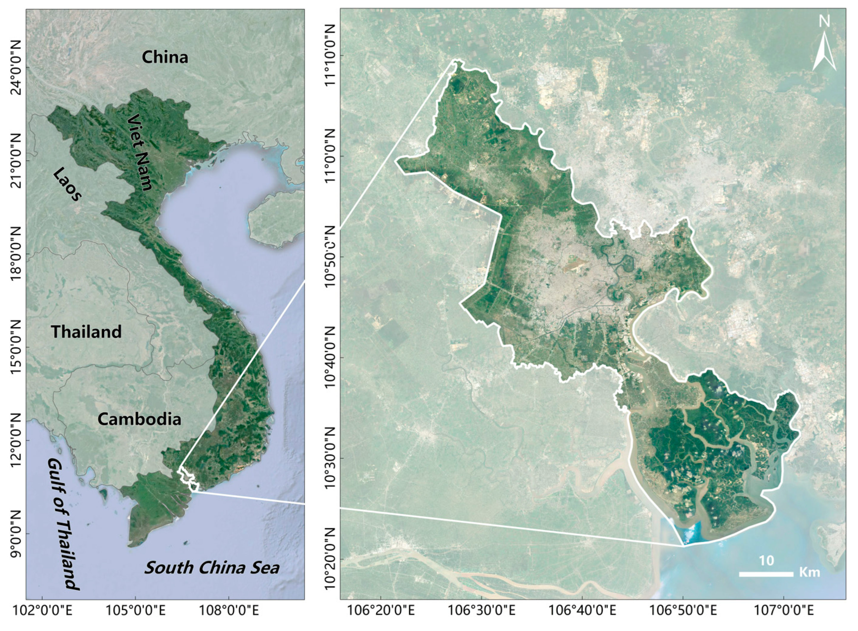
Figure 1. Location map of the study area.
Sustainability 15 06798 g001
Figure 2. Samples distribution of land cover training (left) and land cover verification (right).
Sustainability 15 06798 g002
Figure 3. Before (a) and after (b) composite of band combination 764 with band Pan.
Sustainability 15 06798 g003
Figure 4. Before (a) and after (b) composite of band combination 543 with band Pan.
Sustainability 15 06798 g004
Figure 5. The flow chart for land cover classification using two band combinations and three machine learning algorithms.
Sustainability 15 06798 g005
Figure 6. Flowchart of BPNN algorithm.
Sustainability 15 06798 g006
Figure 7. Flowchart of SVM algorithm.
Sustainability 15 06798 g007
Figure 8. Flowchart of R.F. algorithm.
Sustainability 15 06798 g008
Figure 9. Land cover classification of Ho Chi Minh City based on Lnadsat8-OLI Image data and BPNN algorithm, band combination 764 (a), band combination 543 (b).
Sustainability 15 06798 g009
Figure 10. Land cover classification of Ho Chi Minh City based on Lnadsat8-OLI Image data and SVM algorithm, band combination 764 (a), band combination 543 (b).
Sustainability 15 06798 g010
Figure 11. Land cover classification of Ho Chi Minh City based on Lnadsat8-OLI Image data and R.F. algorithm, band combination 764 (a), band combination 543 (b).
Sustainability 15 06798 g011
Figure 12. Classification of land cover in Ho Chi Minh City, Sentinel-2 land cover data product (a), Globalland30 land cover data product (b).
Sustainability 15 06798 g012
Figure 13. The difference in land cover classification results (the red line is vegetation classification difference, the blue line is vegetation and Built-up Area misclassification). (a1,b1) are band combination 764 classification, (a2,b2) are band combination 543 classification, (a3,b3) are Google images of corresponding positions.
Sustainability 15 06798 g013
Figure 14. In a regional comparison of the Built-up Area, (a1,b1) are classified as band combination 764, (a2,b2) as band combination 543, and (a3,b3) are Google images at the corresponding locations.
Sustainability 15 06798 g014
Figure 15. Comparison of shadow recognition and Water for buildings and tall trees in the Built-up Area, (a1,b1) are classified by band combination 764, (a2,b2) are classified by band combination 543, and (a3,b3) are Google images of the corresponding locations.
Sustainability 15 06798 g015
Figure 16. Comparison between the classification results of three machine learning algorithms and actual ground objects: (a,e) are the classification results of the BPNN algorithm, (b,f) are the classification results of the SVM algorithm, (c,g) are the classification results of the R.F. algorithm, (d,h) are the actual ground features in the same position.
Sustainability 15 06798 g016
Figure 17. Comparison of classification results with other data products, (a1,b1,c1) are band combination 764 classification results, (a2,b2,c2) are Sentinel-2 classification results, (a3,b3,c3) are globalland30 classification results, and (a4,b4,c4) are the corresponding Google images.
Sustainability 15 06798 g017
Table 1. The number of training samples and verification samples for land cover classification.
ItemsTraining SamplesValidation Samples
Classification
Built-up Area273143
Trees240161
Water236143
Crops255172
Grass150101
Bare Ground202145
Total1356865
Table 2. Jeffries-Matusita coefficient of training samples.
ClassificationBuilt-Up AreaTreesWaterCropsGrassBare Ground
Band764/543764/543764/543764/543764/543764/543
Built-up Area 1.98/1.991.96/1.801.98/1.981.97/1.851.80/1.89
Trees1.98/1.99 2.00/2.001.90/1.872.00/2.002.00/2.00
Water1.98/2.002.00/2.00 2.00/2.002.00/2.002.00/2.00
Crops1.98/1.981.90/1.872.00/2.00 1.81/1.842.00/2.00
Grass1.97/1.852.00/2.002.00/2.001.81/1.84 1.84/1.97
Bare Ground1.80/1.892.00/2.002.00/2.002.00/2.001.84/1.97
Table 3. Jeffries-Matusita coefficient of validation samples.
ClassificationBuilt-Up AreaTreesWaterCropsGrassBare Ground
Band764/543764/543764/543764/543764/543764/543
Built-Up Area 1.99/2.001.98/1.811.99/1.991.98/1.901.91/1.91
Trees1.99/2.00 2.00/2.001.98/1.862.00/2.002.00/2.00
Water1.98/1.812.00/2.00 2.00/2.002.00/2.002.00/2.00
Crops1.99/1.991.98/1.862.00/2.00 1.86/1.922.00/2.00
Grass1.98/1.902.00/2.002.00/2.001.86/1.92 1.76/1.85
Bare Ground1.91/1.912.00/2.002.00/2.002.00/2.001.76/1.85
Table 4. Classification accuracy and Kappa coefficient of Band combination 764 and Band combination 543 using BPNN algorithm.
ClassificationBand Combination 764Band Combination 543
Prod. Acc.
(Percent)
User Acc.
(Percent)
Prod. Acc.
(Pixels)
User Acc.
(Pixels)
Prod. Acc.
(Percent)
User Acc.
(Percent)
Prod. Acc.
(Pixels)
User Acc.
(Pixels)
Crops99.5093.88399/401399/42593.5289.29375/401375/420
Grass92.0795.49360/391360/37777.2495.57302/391302/316
Bare Ground66.9897.26142/212142/14633.0241.9270/21270/167
Trees100.0099.562693/26932693/270598.6399.102656/26932656/2680
Water99.86100.008064/80758064/806499.7899.938057/80758057/8063
Built-up Area100.0097.572209/22092209/226499.1493.792190/22092190/2335
OA99.18%97.63%
Kappa 0.9870.961
Producer’s Accuracy (Prod.Acc.), User’s Accuracy (User Acc.), Overall Accuracy (O.A.), and Kappa coefficient (Kappa) for the classification experiments.
Table 5. Classification accuracy and Kappa coefficient of Band combination 764 and Band combination 543 using the SVM algorithm.
ClassificationBand764Band543
Prod. Acc.
(Percent)
User Acc.
(Percent)
Prod. Acc.
(Pixels)
User Acc.
(Pixels)
Prod. Acc.
(Percent)
User Acc.
(Percent)
Prod. Acc.
(Pixels)
User Acc.
(Pixels)
Crops96.2695.54386/401386/40492.5294.64371/401371/392
Grass94.6398.79370/391370/38291.5695.98358/391358/373
Bare Ground83.9698.34178/212178/18191.5194.63194/212194/205
Trees100.0099.152693/26932693/271699.7898.642687/26932687/2724
Water99.8499.968062/80758062/806599.6799.958048/80758048/8052
Built-up Area99.8698.792206/22092206/223399.5098.342198/22092198/2235
OA99.38%99.11%
Kappa 0.9900.985
Producer’s Accuracy (Prod.Acc.), User’s Accuracy (User Acc.), Overall Accuracy (O.A.), and Kappa coefficient (Kappa) for the classification experiments.
Table 6. Classification accuracy and Kappa coefficient of Band combination 764 and Band combination 543 using R.F. algorithm.
ClassificationBand764Band543
Prod. Acc.
(Percent)
User Acc.
(Percent)
Prod. Acc.
(Pixels)
User Acc.
(Pixels)
Prod. Acc.
(Percent)
User Acc.
(Percent)
Prod. Acc.
(Pixels)
User Acc.
(Pixels)
Crops95.2696.22382/401382/39794.5194.28379/401379/402
Grass95.4095.89373/391373/38996.6895.94378/391378/394
Bare Ground87.2699.46185/212185/18691.0499.48193/212193/194
Trees99.9699.122692/26932692/271699.5599.082681/26932681/2706
Water99.81100.008060/80758060/806099.3999.988026/80758026/8028
Built-up Area99.9198.842207/22092207/223399.9597.832208/22092208/2257
OA99.41%99.17%
Kappa 0.9900.986
Producer’s Accuracy (Prod.Acc.), User’s Accuracy (User Acc.), Overall Accuracy (O.A.), and Kappa coefficient (Kappa) for the classification experiments.
Table 7. Comparison between RF764 land cover classification results, Sentinel-2, and Globalland30 products (km2).
ClassificationRF764Sentinel-2Globalland30
Crops221.74344.471050.69
Trees591.21467.71370.38
Grass299.5924.730.22
Water408.62408.52263.40
Bare Ground35.983.770
Built-up Area554.29862.26426.75
Total2111.452111.452111.45
Table 8. Comparison of land cover classification results in a proportion by three machine learning methods based on band combination 764.
ClassificationBPNNSVMRF
Crops174.83%137.12%100.00%
Trees44.93%87.48%100.00%
Grass123.71%76.57%100.00%
Water86.61%92.27%100.00%
Bare Ground98.78%101.39%100.00%
Built-up Area113.48%100.66%100.00%
Based on the R.F. algorithm classification result area.
Disclaimer/Publisher’s Note: The statements, opinions and data contained in all publications are solely those of the individual author(s) and contributor(s) and not of MDPI and/or the editor(s). MDPI and/or the editor(s) disclaim responsibility for any injury to people or property resulting from any ideas, methods, instructions or products referred to in the content.