Article

Reducing Octane Number Loss in Gasoline Refining Process by Using the Improved Sparrow Search Algorithm

School of Mechanical Engineering, Yangzhou University, Huayangxi Road No. 196, Yangzhou 225127, China
*
Author to whom correspondence should be addressed.
Sustainability 2023, 15(8), 6571; https://doi.org/10.3390/su15086571
Submission received: 27 February 2023 / Revised: 5 April 2023 / Accepted: 11 April 2023 / Published: 13 April 2023

Abstract

:
Gasoline is the primary fuel used in small cars, and the exhaust emissions from gasoline combustion have a significant impact on the atmosphere. Efforts to clean up gasoline have therefore focused primarily on reducing the olefin and sulfur content of gasoline, while maintaining as much of the octane content as possible. With the aim of minimizing the loss of octane, this study investigated various machine learning algorithms to identify the best self-fitness function. An improved octane loss optimization model was developed, and the best octane loss calculation algorithm was identified. Firstly, the operational and non-operational variables were separated in the data pre-processing section, and the variables were then filtered using the random forest method and the grey correlation degree, respectively. Secondly, octane loss prediction models were built using four different machine learning techniques: back propagation (BP), radial basis function (RBF), ensemble learning representing extreme gradient boosting (XGboost) and support vector regression (SVR). The prediction results show that the XGboost model is optimal. Finally, taking the minimum octane loss as the optimization object and a sulfur content of less than 5µg/g as the constraint, an octane loss optimization model was established. The XGboost prediction model trained above as the fitness function was substituted into the genetic algorithm (GA), sparrow search algorithm (SSA), particle swarm optimization (PSO) and the grey wolf optimization (GWO) algorithm, respectively. The optimization results of these four types of algorithms were compared. The findings demonstrate that among the nine randomly selected sample points, SSA outperforms all other three methods with respect to optimization stability and slightly outperforms them with respect to optimization accuracy. For the RON loss, 252 out of 326 samples (about 77% of the samples) reached 30%, which is better than the optimization results published in the previous literature.

1. Introduction

With the continuous development of the economy, the automobile industry has made great progress. However, environmental pollution and energy shortage are becoming increasingly serious. Of these, exhaust gases from petrol combustion have a significant impact on atmospheric pollution, and it is essential to take strict measures. For the development of the petroleum industry, the key is to reduce the sulfur and olefin content of gasoline while maintaining as much octane as possible [1]. In the process of desulphurizing and reducing olefins in fluid catalytic cracking (FCC) gasoline, previous techniques generally reduce the octane number of gasoline [2]. If the octane number is increased by 1 unit, a very significant profit can be made. Therefore, if the octane number loss can be effectively reduced during desulfurization and olefin reduction, the economic benefits can be greatly improved.
During the fuel production process, due to the lack, low reliability or absence of measuring instruments in the production facilities, some technological parameters related to the initial quantitative information about operation of complex chemical engineering systems (CES) cannot be obtained. This makes it very difficult to develop mathematical models and to optimize and manage CES using traditional mathematical techniques. Orazbayev et al. [3] used fuzzy mathematics to address the problem of uncertain initial information and improve the efficiency of the catalytic reforming unit by building a system model and optimizing the operating mode. The operating parameters of the catalytic reforming unit were successfully optimized, and the product quality and output were improved. Ospanov et al. [4] applied fuzzy mathematics methods to the control and optimization of the benzene production process and adopted a decision analysis method to develop a control scheme of technical objects to solve problems in a fuzzy environment. By constructing a model and performing decision analysis, the control and optimization of benzene production process were successfully realized.
In terms of octane number prediction, Pasadakis et al. [5] identified components by Fourier transform infrared spectroscopy and independent component analysis, correlated the spectral variable X with the sample property Y and then calculated the octane number. However, this method has high instruments requirements and is difficult to perform in practice. The mean octane number was predicted by Liu et al. [6] through the establishment of a multi-objective nonlinear optimization model with maximum RON loss reduction and minimum operational risk. Wang et al. [7] used the partial least squares regression method to fit the analysis of gasoline octane number. Due to the highly non-linear and coupling relationship of the data, the prediction accuracy of this method cannot be guaranteed. A new analytical framework for octane number prediction was proposed by Li et al. [8], which used kernel principal component analysis (KPCA) to reduce the dimension of variables in the fluid catalytic cracking (FCC) process, A new analytical framework for octane number prediction was proposed by Li et al. [8], which used kernel principal component analysis (KPCA) to reduce the dimension of variables in the fluid catalytic cracking (FCC) process, support vector regression (SVR) to build the RON prediction model, and particle swarm optimization (PSO) to select the optimal model parameter combination. A RON predictive model that combines a random forest algorithm, a BP neural network and a genetic algorithm has been proposed by Fu et al. [9] to meet the real needs of chemical manufacturing. This method can be used to reduce overfitting and effectively predict octane number and residual value. Furthermore, machine learning-based data mining methods were widely used by some scholars [10,11,12,13,14], and these proposed models were superior to the traditional methods in both accuracy and generalization and achieved better results in predicting octane number.
Many multi-objective optimization problems (MaOPs) exist in real applications, often with many decision variables. Although various methods have been proposed for the solution of MaOPs, the performance of these algorithms degrades significantly as the number of decision variables or objective functions increases. Yao et al. [15] proposed an approach to solve large-scale MaOPs based on dimension reduction and knowledge-guided evolutionary algorithms. With respect to octane number optimization, Cheng et al. [16] proposed the hybrid gray wolf optimizer (HGWO) algorithm; by constraining the objective function of minimizing the RON loss, the optimal value of the characteristic variable could be obtained through continuous iteration. Cui et al. [17] effectively reduced the octane prediction mean square error (MSE) by 5.79% using differential evolution-based parameter optimization. The dragonfly algorithm (DA) was successfully applied to optimize the octane number by Zhang et al. [18]. This combination model can balance the local search and global search, and effectively prevent the algorithm from reaching the local optimal solution. Guo et al. [19] proposed an effective method to reduce the octane number by processing the target product with a multi-objective particle swarm optimization algorithm. Based on the concept of substation engineering data space, Xu et al. The authors of [20] studied the influence factors and developed a static total investment smart forecasting model of substation engineering. To improve the prediction accuracy and convergence speed of the neural network, the sparrow search algorithm (SSA) was used to optimize the parameters of the BP neural network. This proposed method provides a new idea for the study of gasoline octane number optimization.
Although many scholars have conducted much research on octane number optimization, there is still not enough data to prove which specific method is significant for octane number optimization. In terms of variable dimension reduction, principal component analysis has the disadvantages of being sensitive to outliers and not having many variables. The clustering method has the disadvantages of being sensitive to noise points and outliers, and has difficulty in determining the initial clustering center. In terms of prediction and optimization, when using neural networks, XGBoost, and genetic algorithms, the prediction and optimization effect of dynamic changes is often not good. In general, non-linear constraints on the actual sulfur content limit need to be considered for octane reduction models in gasoline refining. Based on the related research [20], this paper introduces the sparrow algorithm in the direction of gasoline octane prediction for the first time, and establishes the gasoline octane loss optimization model, which is combined with the sparrow algorithm to form a new algorithm. It can effectively improve the accuracy of gasoline octane prediction.
Firstly, the dimensions of the operational variables and non-operational variables were reduced using random forests and grey correlation, respectively. Then, the octane prediction results of back propagation (BP) [21], radial basis function (RBF) [22], extreme gradient boosting (XGboost) [23] and support vector regression (SVR) [24] were compared to determine the optimal adaptive function. Finally, the traditional genetic algorithm (GA) [25], particle swarm optimization (PSO) [26,27] and grey wolf optimization algorithm (GWO) [28] were compared with the sparrow search algorithm (SSA) [29] introduced in this study, and the numerical optimization results were compared with the empirical data set and other optimization results published in the related literature. The results show that, in terms of optimization results and stability, the SSA algorithm is superior to the other three algorithms.
The main contributions made by this paper are as follows: (1) A hybrid method was proposed to filter the variables and reduce variable dimensions; (2) the machine learning algorithm with the best prediction results was introduced into the optimization fitness function to realize the optimization calculation; (3) to solve the octane loss optimization model, the problem of solving the minimum octane loss value was transformed into solving the maximum octane product value; (4) the SSA algorithm was introduced into the nonlinear optimization problem with higher stability than other traditional heuristic algorithms.
The remaining sections are organized as follows: Section 2 presents the pre-processing of the original data. Section 3 is a description of the methods used in this paper and the overall modelling process. Section 4 presents the results obtained. Section 5 discusses the results. Section 6 concludes the entire work and gives an outlook for future work.

2. Data Processing

The public dataset used in this paper is provided by the Sinopec Gaoqiao Petrochemical real-time database (Honeywell PHD) and the LIMS experimental database [30]. The data of operational variables were collected from April 2017 to May 2020, and were collected from 354 operational points. The data collection frequency was every 3 min from April 2017 to September 2019, and every 6 min from October 2019 to May 2020. The raw material, product and catalyst data were collected from the LIMS experimental database from April 2017 to May 2020. The octane number of raw material and product is an extremely important variable for modeling, and the frequency of the data collection was twice a week.
The database contains 325 samples from a Chinese petrochemical company’s petrol refining line. It contains 7 raw material variables, 4 adsorbent variables, 2 product variables (these are non-operational variables) and 342 operational variables. In the process of collecting original data, most of the data is in line with the actual situation. Meanwhile, due to a series of adverse effects such as environmental mutations, some of the collected data is not in line with the actual situation. There are two types of abnormal data in this part: missing data and anomalous data. At the same time, the dimension of the data is too large, so, in order to remove redundant variables, it is necessary to reduce the dimension of the data.

2.1. Processing of Missing Data

By finding and deleting missing data, the negative influence of missing data on the gasoline octane prediction below can be eliminated. In the case of missing samples, the processing method can be defined as follows:
n n o n e = 0 , Sample   complete 0 < n n o n e 10 ,   Sample   alternative   m i n n o n e > 10 ,   Sample   missing   m j
in which nnone is the number of missing samples in a column, mi and mj represent the sample that can be replaced and the sample that can be directly deleted, respectively. i and j represent the serial number of the samples. If the number of missing samples in a column nnone is 0, this column is not processed. If the number of missing samples in a column nnone ∈ (0, 10), it is replaced by linear interpolation of two neighboring data. When the number of missing samples nnone ∈ (10, +∞), the entire column is deleted.

2.2. Processing of Anomalous Data

Based on the elimination of the missing data, anomalous data hidden in the remaining data are found and deleted, which can eliminate the negative impact of anomalous data on the gasoline octane prediction below.
The Bessel formula [31] can be used to calculate the standard error σ for the anomalous data. If the error of the data is not within the range of the Bessel formula, it can be identified as anomalous data, and the relationship can be represented by:
σ = [ 1 n 1 i = 1 n v i 2 ] 1 / 2 = i = 1 n x i i = 1 n x i / n 2 / ( n 1 ) 1 / 2
where x is the arithmetical mean; vi is the residual error, vi = xix (i = 1, 2, …, n). When the residual error vi (1 ≤ in) of a measured value xi satisfies |vi| = |xix| > 3σ, xi is considered to be an anomalous value with a large error value and should be eliminated.

2.3. Data Dimension Reduction

The number of data dimensions to be filtered is too large, while the sample size is too small. In this paper, operational variables and non-operational variables were separated and filtered, respectively. For operational variables, due to the small dimension of the variables, the random forest method [32] was used for filtering, which can avoid overfitting. For the non-operational variables, due to the large dimension, the grey correlation degree method [33] combined with the Pearson correlation coefficient method [34] was used for data filtering. At the same time, the proposed method was also compared with the simple grey correlation degree to determine the better filtering method. The specific filtering method is shown in Figure 1:
To eliminate the influence of the quantity dimension, the data should be normalized [35] after preprocessing, and the method can be expressed as follows:
x n o r m = x x min s
in which xnorm is the normalized data, x is the variable data value, xmin is the minimum value of the variable data, xmax is the maximum value, s is the difference of the sample values, which is of the form s = xmaxxmin.
The results of random forest and grey correlation degree filtering are as follows:
H ( x ) = arg   max Y K = 1 n I ( h i ( x ) = Y )
G ( x ) = arg max ( γ i ( x 0 , x i ) ) = arg max ( 1 n k = 1 n γ ( x 0 ( k ) , x i ( k ) ) )
where H(x) is the filtering decision result of the random forest method. hi(x) is the prediction and filtering result of each decision tree classifier. Y is the filtering target. I(hi(x) = Y) is a characteristic function. G(x) is the result of the grey correlation degree filtering decision. γ(x0, xi) is the value of the grey correlation degree filtering. x0 is the target variable. xi is the current variable; argmax is the maximum set of filtering values; x0 and xi are the elements of the target and current variables.
The results of the grey correlation degree filtering are recorded as G0, and the results of the mixed filtering variables are recorded as C0, with the elements in the C0 and G0 sets kept equal.
The Pearson correlation coefficient can be used to evaluate the results of variable filtering. It describes how close a relationship exists between two remote variables, in this case to measure the linear correlation between variables X and Y. Its value lies between (−1, 1) and is generally expressed by rxy, which can be calculated as follows [36]:
r x y = ( n X Y X Y ) n X 2 ( X ) 2 n Y 2 ( Y ) 2
where n denotes the number of samples, X, Y represent the value of two variables. The two variables are positively correlated if r > 0; if r = 0, it means that the two variables are irrelevant; if r < 0, then there is a negative correlation between the two variables. The stronger the correlation, the higher the absolute value of r. The correlation can be judged according to the value interval, and it is considered that if the absolute value of r is between (0.8, 1), it is a very strong correlation; if the absolute value of r is between (0.6, 0.8), it is a strong correlation; if the absolute value of r is between (0.4, 0.6), it is a moderate correlation; if the absolute value of r is between (0.2, 0.4), it is a weak correlation; if the absolute value of r is less than 0.2, it is a very weak correlation or uncorrelation.
At the same time, the correlation degree rRON (product octane number) is defined as the criteria for filtering variables. Its calculation formula is as follows:
r R O N = i = 1 n r x i · R O N
where n is the number of samples filtered. rxi·RON is the degree of correlation between this variable and the product octane number, xi = {C0, G0}.

3. Method

After determining the main variables, four typical machine learning algorithms, BP neural network, RBF neural network, XGBoost and the SVR algorithms, were used to build the octane loss prediction models. The performance of these models was evaluated. Combined with the octane loss optimization model proposed in this study, the XGBoost prediction model was selected as the fitness function and substituted into the genetic algorithm (GA), sparrow search algorithm (SSA), particle swarm optimization algorithm (PSO) and the grey wolf optimization (GWO) algorithm, respectively, to optimize the octane loss model.

3.1. Development of Octane Number Prediction Model

Using RON as the target variable, four machine learning algorithms, BP, RBF, XGBoost and SVR, were used to establish machine learning models; these algorithms are introduced below.
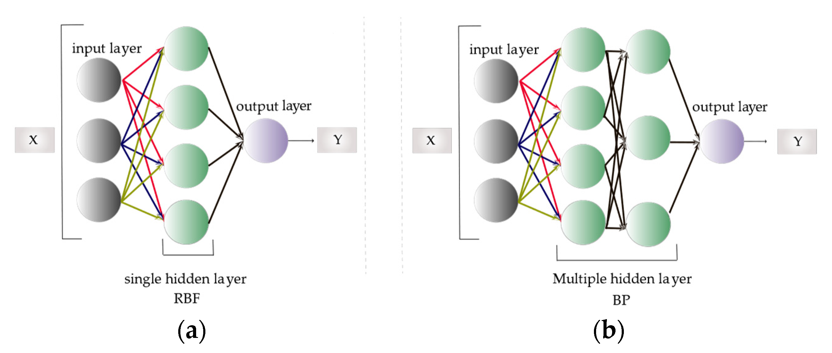
The BP network is based on the error backpropagation algorithm, which is the most widely used algorithm. Each topology structure is realized in a fully connected way, and the neurons in the same layer are disconnected from each other. Generally, there is at least one hidden layer, and sigmoid is used as the activation function for downward propagation. Radial basis function (RBF) network is a type of forward network based on function approximation theory. The main difference between RBF and BP is the difference in the activation function. The activation function of RBF is a radial basis function, and the nodes of the hidden layer produce local responses to the input. Therefore, the hidden layer is also known as the local perceptual network [37,38]. The linearly weighted sum of the output of the neurons in the hidden layer is the output of the two network models above. The prediction model is shown in Equation (8). Each layer of the neural network consists of several neurons. As the signal is transmitted to each neuron, a new output signal is transmitted to the next layer of neurons by transforming some form of the excitation function. The topology diagrams of the two neural networks are shown in Figure 2.
As a representative of ensemble learning, the XGBoost algorithm model is effectively improved based on the original gradient lifting decision tree GBDT [39]. It uses a training set and a real sample to train a tree, and then uses that tree to predict a training set. The “residual” obtained by subtracting the predicted value from the actual value is used to continue training the next tree. The final output will be the sum of the outputs of each training instance, thus improving the overall performance of the model. The objective function is made up of a loss function and a regularization term, as shown in Equation (8).
SVR [40] is a machine learning method. It is based on statistical learning theory and the principle of structural risk minimization. The optimal classification hyperplane is constructed by non-linear mapping of the input to a high-dimensional space. The loss function is minimized to determine the relevant model by constructing a loss function between the sample label and the predicted value of the model. The prediction model is shown in Equation (8).
Based on the above four methods, the prediction models can be written as follows:
BP : y j = f ( i = 1 S i ω k j r i + b k ) RBF : y j = i = 1 n w i j α i ( x ) b i XGBoost : y j = i l ( y ^ i , y ¯ i ) + k ( f k ) , where   ( f ) = γ T + 1 2 λ ω 2 SVR : y j = i = 1 n W i φ ( x ) + b k
In Equation (8), for the BP and RBF methods: where yj is the output of the neurons, ri is the node of the hidden layer, ωij is the connection weight of the neurons between the hidden and output layers. bi is the connection threshold between the hidden and output layers, f is the transfer function, αi(x) is the radial basis function. For the objective function of XGBoost method, ŷi is the predicted value of the model, ӯi is the category label of sample i, k is the number of trees, fk is the model of a tree k, T is the number of nodes of each leaf, l(ŷi, ӯi) is the loss function, Ω(fk) is the regular elements, ω denotes the set consisting of the scores of each leaf node, γ is the first regularization coefficient, namely the training error, λ represents the second regularization coefficient, which is the sum of the complexity of the trees. For the SVR method, where W is the weight vector, φ(x) is the implicit mapping function, x is the sample feature vector in original space, bk is the bias term.
In the process of data prediction by using the above models, due to certain errors between the predicted and actual value, the following two methods were adopted in this study to measure the prediction accuracy: root mean square error (RMSE) and goodness of fit (R2) [41], which can be expressed as:
R M S E = 1 m i = 1 m ( y i y ^ i ) 2 R 2 = 1 i = 1 m ( y i y ^ i ) 2 i = 1 m ( y i y ¯ i ) 2
where m and n are the number of samples to be taken, yi is the actual value, ӯi is the average of the actual values, ŷi is the predicted value.
In this paper, BP, RBF, XGBoost and SVR were used to predict the octane number of gasoline. Combined with the evaluation indexes, RMSE and R2, the method with the highest prediction accuracy is determined. The model with the highest prediction accuracy is then used as the fitness function of the improved optimization algorithm to calculate the subsequent gasoline octane rating.

3.2. Establishment of Octane Number Loss Optimization Model

An improved model has been proposed in this section, which aims to accurately represent the octane loss of gasoline, the product octane number and the feedstock octane number, in order to reduce the negative impact of calculation errors on the prediction results.
With the minimum RON loss as the target and a sulfur content of less than 5% as the constraint condition, an optimization objective function has been established, which is shown in Equation (10)
min   R O N l o s s ( X i ) s . t S ( X i ) 5   µ g / g min X i < X i < max X i , i = 1 , 2 , 3 , , n
where Xi is the decision variable, RONloss(Xi) is the loss quantity of RON. The RON loss quantity can be expressed as the difference between RON raw materials and RON products, which can be expressed as:
R O N l o s s ( X i ) = R O N raw R O N product ( X i )
where RONproduct(Xi) is the product RON, RONraw is the raw material RON, which is the non-operational variable and can be used as a fixed value. Therefore, the objective function can be transformed into:
min   R O N l o s s ( X i ) = min [ R O N raw R O N product ( X i ) ] = R O N raw max [ R O N product ( X i ) ]
The final optimization function can be obtained by further simplifying the above equation:
max   R O N product ( X i ) s . t S ( X i ) 5   µ g / g min X i < X i < max X i , i = 1 , 2 , 3 , , n
where RONproduct(Xi) and S(Xi) can be expressed as the product octane number and product sulfur content fitted by the optimal model, respectively, which can be further expressed as:
R O N product ( X i ) = g ( x 1 , x 2 , x 3 , , x i 1 , x i ) S ( X i ) = h ( x 1 , x 2 , x 3 , , x i 1 , x i )
where g and h represent the optimal model mapping, and determining the optimal model mapping can be expressed as:
R O N product ( X i ) m a p p i n g max R 2 B P , R 2 X G boost , R 2 S V R , R 2 R B F S ( X i ) m a p p i n g max R 2 B P , R 2 X G boost , R 2 S V R , R 2 R B F
In the above formula, R2 indicates goodness of fit, R2 in the full set (test set + training set) is used as the basis for selection, the model with the most accurate prediction (R2 is closest to 1) among BP, XGBoost, SVR and RBF is selected as the mapping function.
Finally, the magnitude of the RON loss η can be calculated using the following formula:
η = ( R O N raw R O N product ) [ R O N raw R O N product ( X i ) ] R O N raw R O N product × 100 %
where RONraw is the product octane number before optimization, RONproduct(Xi) is the product octane number fitted by the optimum model, and RONproduct is the product octane number after optimization. Therefore, the optimized improved octane calculation model can be expressed as:
max   R O N product ( X i ) s . t S ( X i ) 5   µ g / g min X i < X i < max X i , i = 1 , 2 , 3 , , n η = ( R O N raw R O N product ) [ R O N raw R O N product ( X i ) ] R O N raw R O N product × 100 % R O N product ( X i ) m a p p i n g max R 2 B P , R 2 X G boost , R 2 S V R , R 2 R B F S ( X i ) m a p p i n g max R 2 B P , R 2 X G boost , R 2 S V R , R 2 R B F

3.3. Improvement and Selection of the Optimization Algorithm

The final results of the model are greatly influenced by a number of sensitive parameters in the forecasting process. The optimal result can be achieved by adjusting these sensitive parameters. For the solution of the optimization model, in addition to comparing the traditional GA, PSO and GWO algorithms, this paper introduces a new intelligent algorithm, SSA algorithm, for comparison, and proposes an optimal octane number optimization scheme.
The SSA algorithm is a new intelligent algorithm that was proposed by Xue et al. [29] in 2020, inspired by sparrow foraging and predation behavior. The method has been gradually applied to unmanned aerial vehicle (UAV) route planning [42], servo system identification and control [43] and random network configuration [44], which has achieved good optimization results. Sparrows are social animals, so when the population is attacked by predators, they will show strong resistance to predation. Thus, sparrows can therefore be classified into three roles: producer, predator and scout [45].
Like other heuristics, it starts with a random population of sparrows and can expect n sparrows in the D-dimensional search space [29]. The fitness value of a bird (target RON) is expressed as follows:
F x = f [ x 1 , 1 x 1 , 2 x 1 , j ] f [ x 2 , 1 x 2 , 2 x 2 , j ] f [ x i , 1 x i , 2 x i , j ]
where f is the individual fitness score. Producers are the more adaptable sparrows in the population. They can forage in a wide range of areas and lead the whole population in the right direction. During each iteration, the position of the producer is updated as follows [42]:
X i , j t + 1 = X i , j t e i α i t m , i f : R 2 < S T X i , j t + G L , i f : R 2 S T
where t is the number of iterations at the current time. Xi,j represents the i-th sparrow’s position information in the j-th dimension, α represents the random numbers in the range of [0, 1], itm is the maximum iterations, G describes the normally distributed randomness, L is a 1 × d matrix in which each element has a value of 1. In this case, R2 is the alarm value ranging from [0, 1], ST is a safety threshold within [0.5, 1]. Predators also need to watch the producers. If it finds that the producer has good food, it will immediately move closer to that position in order to compete for food, making itself a producer. The predator’s position is updated as follows [43]:
X i , j t + 1 = G e X w t X i , j t i 2 , i f : i > n 2 X p t + 1 + X i , j t X p t + 1 A + L , i f : i n 2
where Xp is the producer’s best position, Xwt is the current worst global position of the producer, A is a 1 × d matrix with elements that are randomly assigned to be 1 or −1. A+ can be expressed as A+ = AT(AAT)−1. If a predator does not have access to a food-rich location, it must expand its flight range to get more food. The adaptive function of the sparrow algorithm can be expressed as follows:
F i t ( x ) = f ( X G B o o s t ( x ) )
where Fit(x) is fitness function, XGBoost(x) is the black box function of the model with the highest prediction accuracy.
The GA algorithm was proposed in the 1970s and has become a relatively complete evolutionary algorithm [25]. Based on biological natural selection and population evolution, the algorithm exchanges chromosome information in the population through iterative changes by selection, crossover and variation. Finally, a chromosome that satisfies the optimization requirements is generated, and the search process is adaptively controlled to obtain the best solution.
The product octane number and raw material octane number are coded by the genetic algorithm to realize the one-to-one correspondence between population and individual. Additionally, according to the gene coding method, a series of gene sequences are generated to form the corresponding individuals, and a certain number are generated to form the initial population. In addition, it is also necessary to use fitness function, through the roulette algorithm and the optimal individual preservation of the selection operator to carry out genetic iteration, to achieve the goal of minimum gasoline octane loss. The main relations of the genetic algorithm are:
K i , j = i = 1 i max R O N The   coding   process F i t ( x ) = f ( X G B o o s t ( x ) ) T h e   fitness   function P i = F i t ( x i ) i = 1 m F i t ( x i ) Iteration   of   genetics
where K represents the corresponding code, if j = 1, RON is RONraw; when j = 2, RON is RONproduct. Fit(x) is the fitness function, XGBoost(x) is the black box function of the model with the highest prediction accuracy, Pi is the probability of inheriting a new population.
The PSO algorithm [26,27] was proposed in the 1990s and was inspired by bird predation. When birds hunt, they usually look for the nearest area. Each particle in this algorithm represents a potential solution, its movement speed determines its movement, and its speed is dynamically adjusted with its own and other particles’ movement experience to achieve particle optimization within a region. The relationship can be expressed as:
v i j ( t + 1 ) = ω v i j ( t ) + c 1 r 1 [ p i j ( t ) x i j ( t ) ] + c 2 r 2 [ p g j ( t ) x i j ( t ) ] v i j ( t + 1 ) = x i j ( t ) + v i j ( t + 1 )
where c1 and c2 are acceleration coefficients, r1 and r2 are random numbers in [0, 1], pij(t) is the optimal position for searching the i-th particle swarm, v is the velocity, ω is the control parameter of particle motion inertia, x(t) is the current position of the particle. The inertia weight of PSO is linearly decreased, and the asynchronous linear method is used to improve the learning factor and the inertia weight. Their relationship is as follows:
ω ( k ) = ω 1 ( ω 1 ω 2 ) k G c 1 = c 1 min + k ( c 1 max c 1 min ) G c 2 = c 2 min + k ( c 2 max c 2 min ) G
where ω1 is the initial maximum inertia weight, ω2 is the final minimum inertia weight, which in this paper is 0.4, k is the current number of iterations, G is the maximum iterated number s, cimax and cimin are the maximum and minimum values for ci. Both crossover probability and mutation probability are replaced by adaptive function, and the relationship is the same as Equation (21).
The grey wolf algorithm simulates the grey wolf’s unique hunting and scavenging characteristics [28], completing the task through wolf cooperation. In general, the hunt is completed by tracking, chasing and attacking. During the operation of the GWO algorithm, with each iteration, the wolf’s location is constantly updated. It then selects the positions of different wolves according to the fitness function, guides other wolves to move towards the prey, and finds the prey after several iterations. The relationship is as follows:
D i = r X i ( t ) X ( t ) The   distance   function X i ( t + 1 ) = X i ( t ) A i D i The   position   function Z = 1 n i = 1 n X i ( t + 1 ) The   objective   function F i t ( x ) = f ( X G B o o s t ( x ) ) The   fitness   function
where Di is the distance between the target object and track targets, t is the number of iterations in progress, r and Ai are the coefficient vectors, Xi(t) is the position of the target object, X(t) is the position of the target object being tracked, Z is the final position.
In this study, the traditional GA algorithm, the PSO algorithm and the GWO algorithm, as well as the proposed SSA algorithm [46], were used to optimize the octane number. The best prediction model trained in the previous section was used as the fitness function of the above algorithms. The specific procedure is shown in Figure 3.
In this paper, GA, SSA, PSO and GWO methods are selected and combined with the best methods in Section 3.1 to form optimization and improvement methods, respectively. Combined with the improved optimization model described in Section 3.2, the gasoline octane number can be predicted. By comparing the prediction results of the four optimization methods, the optimal method is selected.

4. Results

4.1. Results of the Feature Parameter Selection

Part of the data after processing is shown in Table 1. The dimension m of the original data is 355. 2 groups of abnormal data and 28 groups of missing data have been removed. Following this, the data dimension m is 325 and the sample size n is 326.
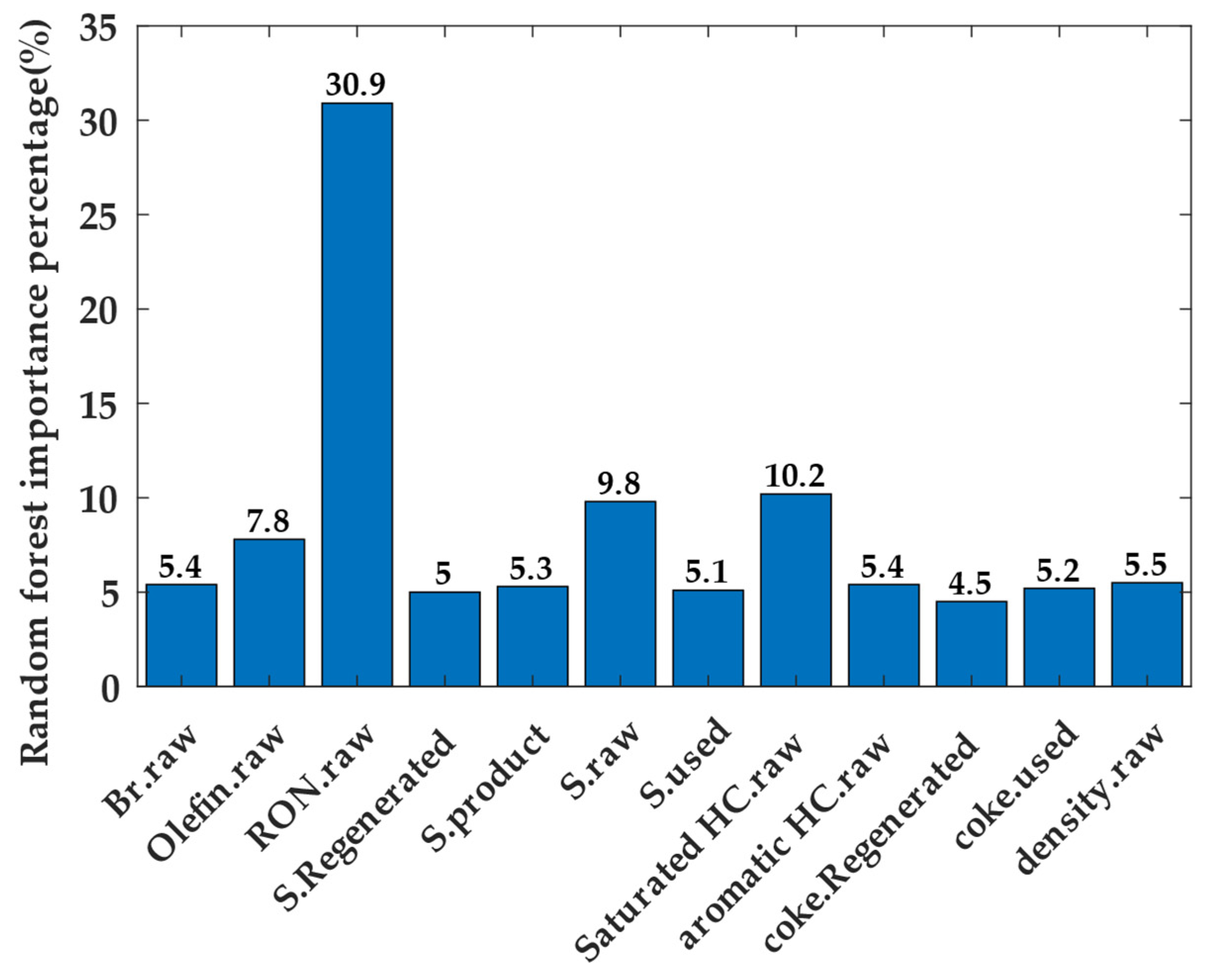
Table 1 shows the data after processing, which includes 313 operational variables and 12 non-operational variables. The random forest method was used to filter the non-operational variables that are closely related to the product RON, and the filtering results are shown in Figure 4:
As shown in Figure 4, four important variables are selected from 12 operational variables. Raw material RON is the most important for product RON, ranking first among all variables and accounting for 30.9%, followed by raw material saturated hydrocarbons, raw sulfur content, and raw olefins, which can be identified as the main filtering results. Regarding the grey correlation degree filtering, the results are presented in Table 2:
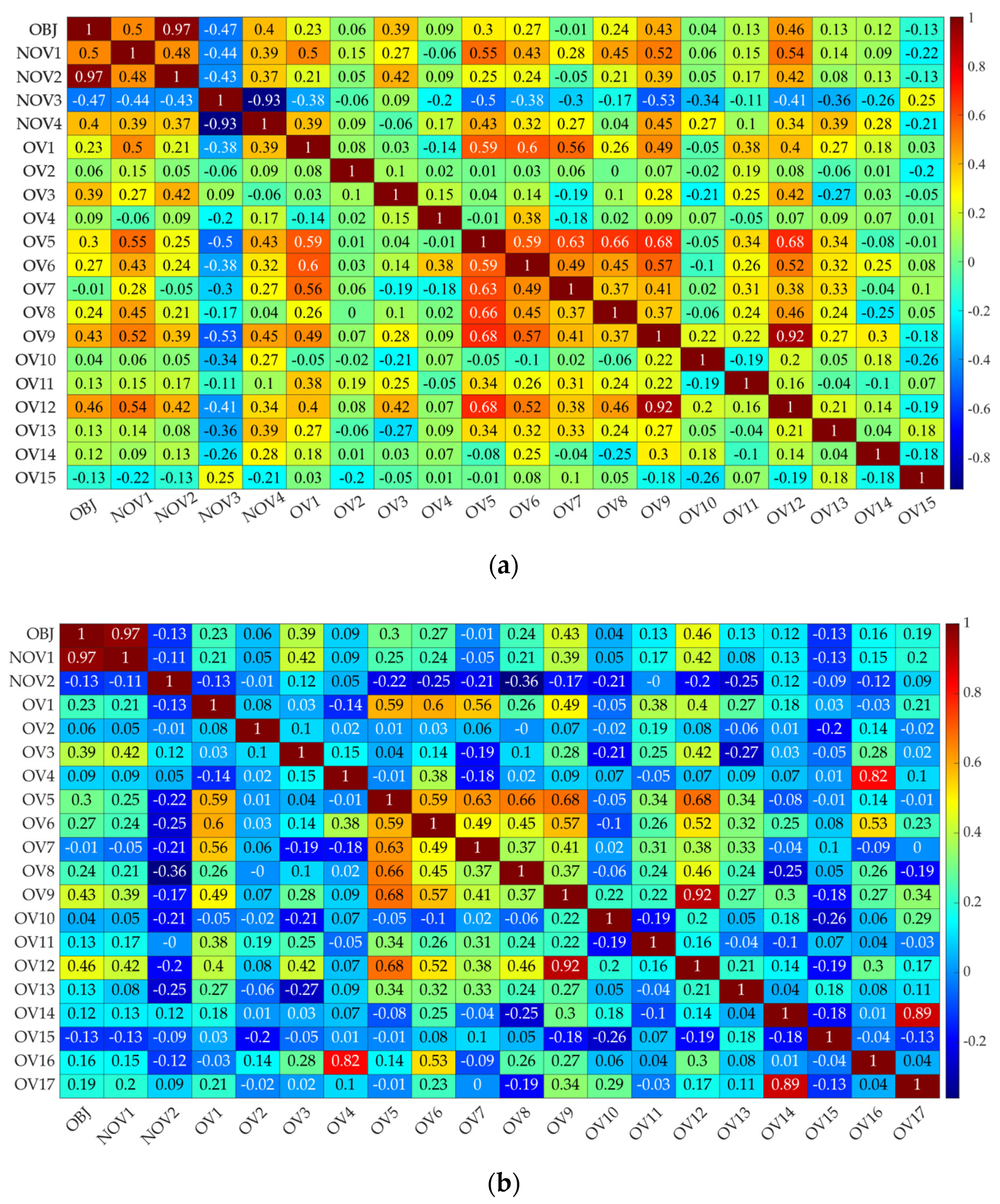
To ensure the consistency of the data, 19 variables were uniformly filtered out by the two methods mentioned in Figure 1. According to Figure 1a, 19 variables with a correlation greater than 0.759 were selected, of which 2 are operational variables and 17 are non-operational variables. The Pearson correlation coefficients of the two screening methods were plotted, as shown in Figure 5.
According to Figure 5 and Equation (6), the total correlation degree between each method and the RON of the product was calculated. Among them, the total correlation degree of method (a) is 6.34, and that of method (b) is 5.46. The mixed filtering method has a better effect, so in this study, 4 operational variables and 15 non-operational variables were filtered by method (a). The filtering results and the corresponding data range are shown in Table 3.
In this paper, the number of samples used is 325, and the data of the prediction model have been divided, with the training set accounting for 0.7 (228 in total). The test set accounts for 0.3, with a total of 97 copies.

4.2. Results of the Prediction and Optimization

4.2.1. Prediction Result of Gasoline Octane Number

After several parameter adjustments, the training results and the main parameters defined in four prediction models are shown in Table 4 and Table 5:
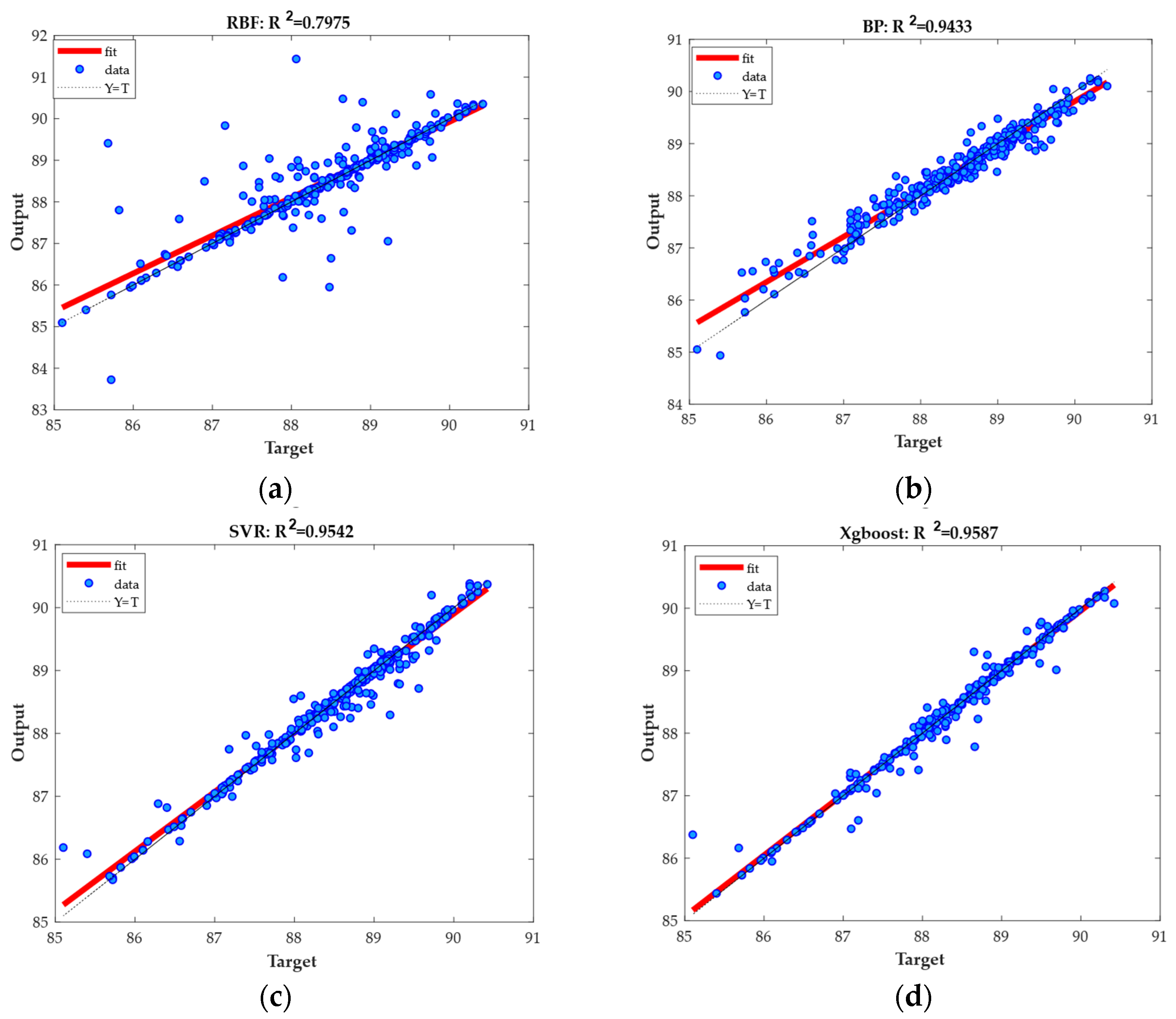
At the same time, the data from the test and training sets were combined to plot the R2 of the four methods and the prediction curves, as shown in Figure 6:
By comparing the above four prediction results, it was found that XGBoost had the highest accuracy in predicting both the octane number and the sulfur content of the products; therefore, the XGBoost model was used as the fitting function to calculate the octane number.

4.2.2. Optimization Results of the Gasoline Octane Number

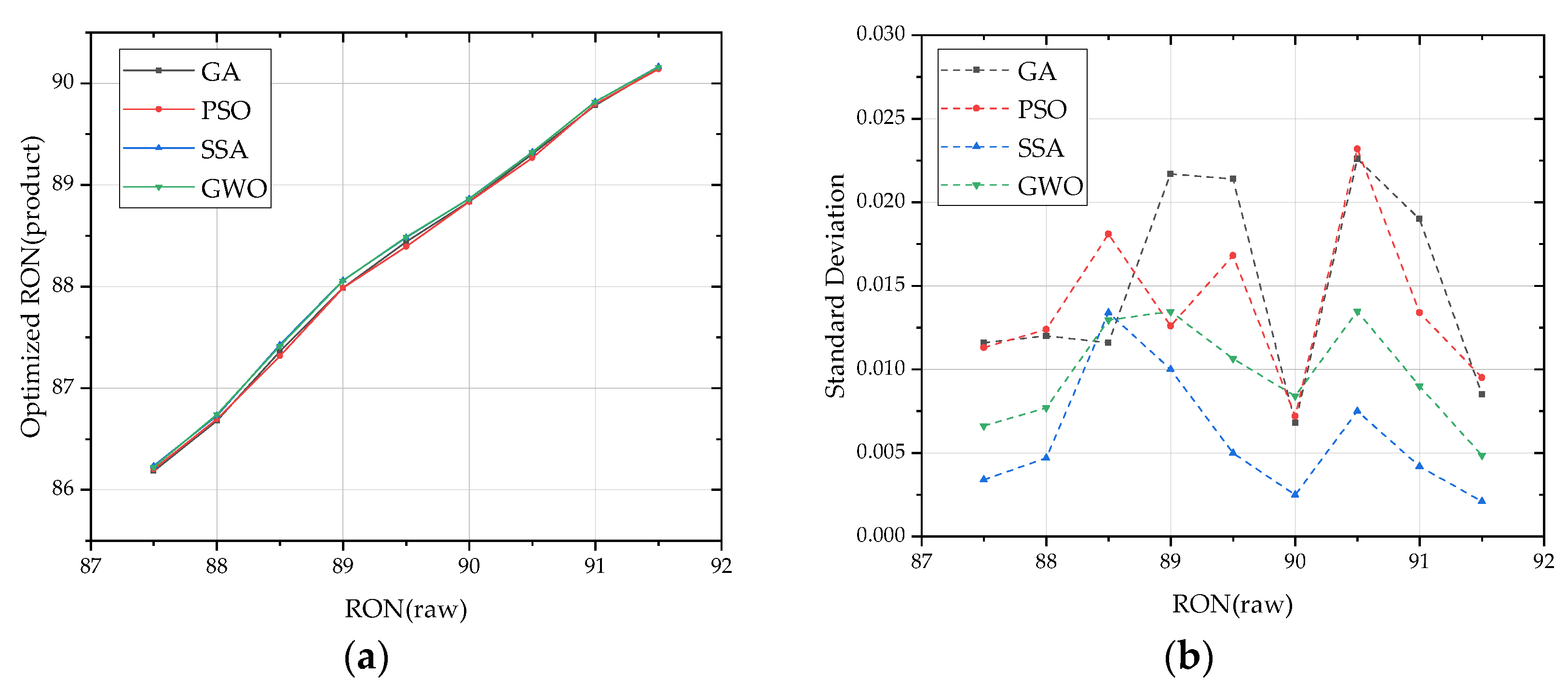
According to the above optimization process, combined with the range of raw material RON variables given in Table 5 (87.2, 91.7), the variation of raw material RON starts from 87.5 with an increasing sub-step of 0.5 and ends at 91.5, the final optimization values of the above 9 points were simulated respectively. At the same time, the experiments were independently repeated 10 times at each point to test the stability of the three algorithms and to eliminate random errors. The mean value of the final convergence results and the standard deviation of the results were calculated for 10 times. The results are shown in Figure 7.
It can be seen in Figure 7a that the curves using the SSA and GWO methods are slightly higher than those using the GA and PSO methods. The overall trend of the three curves is not very different. As shown in Figure 7b, the SSA curve is significantly lower than those of GA, PSO and GWO. At the same time, in Figure 7a,b, the octane numbers obtained by GA and PSO are not significantly different.
In terms of octane number optimization shown in Figure 7, the SSA optimizer outperforms the other three optimizers on six points. In terms of stability, SSA also has certain advantages, which obtained better results than other three algorithms in eight points, further proving that the SSA-based optimization has the advantages of good stability and strong global search ability.

5. Discussion

Regarding model prediction, it can be seen from Table 5 and Figure 6 that BP’s prediction accuracy is higher than RBF in the neural network domain. Although RBF has a better generalization ability, its complexity makes it inferior to the BP neural network in the same prediction range. In the process of parameter optimization, XGBoost adopts the first and second derivatives, and adds the regular term to control the overfitting problem, which effectively improves the model’s predicting accuracy. Therefore, XGBoost is better at predicting nonlinear problems than the other three algorithms.
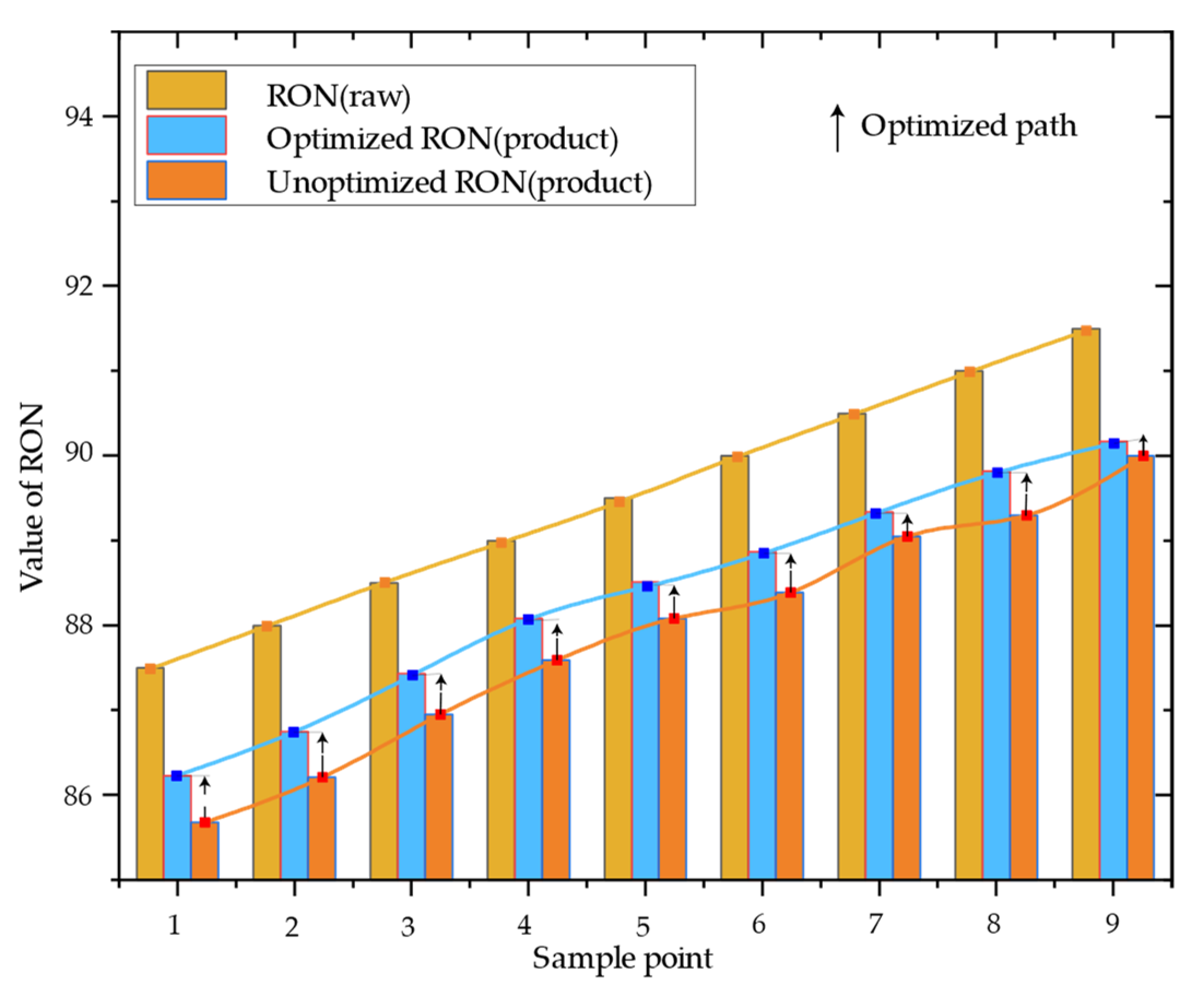
According to Figure 7, it is found that SSA is the best optimization algorithm. Taking the octane number of raw materials as a reference, the octane number of products before and after optimization by the SSA algorithm were compared, as shown in Figure 8.
As shown in Figure 8, the octane number of the raw materials and the RON curves of products before and after optimization were provided.
The arrows show the path of change before and after optimization. According to Equation (17), among the nine sample points tested, the RON loss of seven sample points decreased by 30%, indicating a good optimization effect.
At the same time, the results obtained are competitive compared with other optimization results published in the previous literature. For example, for the RON loss, in literature [6], the octane loss of 245 out of 325 sample points (about 75%) decreased by 30%; in the literature [18], out of the 291 samples, 163 samples had 30% decrease in RON loss, a proportion of about 56%. Corresponding results were obtained in this study: 252 out of 326 samples (about 77% of the samples) reached 30%, meaning the proposed model can achieve better results than the existing literature, which provides a new method for solving nonlinear problems.

6. Conclusions

In this study, the optimization of octane loss in the gasoline refining process has been studied in detail using the Honeywell PHD and LIMS real-time database. From the work carried out in this paper, the following conclusions can be drawn:
Firstly, after pre-processing the data using methods such as the Bessel formula, the main variables were divided into operational variables and non-operational variables, and then processed by using random forest and grey correlation analysis, respectively, which improves the accuracy of the data processing. By comparing the variable filtering methods—grey relational degree-based method and the hybrid filtering method—it can be seen that the hybrid filtering method obtained a better result.
Secondly, in terms of octane number prediction, the prediction results of neural networks, such as BP and RBF, integrated learning XGBoost and SVR regression, were compared, and it could be found that the XGboost model received the best results, which was taken as the fitness function and substituted into the optimization algorithms to perform the RON calculation.
Thirdly, a new optimization model for gasoline octane loss was proposed and integrated into the SSA algorithm. The introduced SSA algorithm was compared with the GA, PSO and GWO, and it was found that the optimization results of the improved SSA algorithm were superior to the other three algorithms. For the RON loss under the condition that the sulfur content is less than 5 µg/g, 252 out of 326 samples (about 77% of the samples) reached 30%, which is better than the optimization results published in the previous literature [6,18].
Finally, the work completed in this paper can provide inspiration for problems such as: data dimension reduction, correlation analysis, value prediction and system optimization and so on. The predictive model proposed in this paper can be used for areas such as: fault diagnosis of rolling bearings, inventory prediction, pollution concentration optimization and traffic accident detection and so on. By using the optimization method, the model parameters can be optimized, which can also be used for path planning, combinatorial optimization and machine learning parameter optimization. However, there are some challenges in solving optimization problems, such as: low convergence accuracy, easy falling into local optimality and sensitivity to parameterization; these need further investigation.

Author Contributions

Conceptualization, J.C.; methodology, J.C.; software, J.Z. and X.Q.; validation, W.X., J.Z. and X.Q.; formal analysis, J.C.; investigation, W.X. and J.Z.; resources, J.C.; data curation, X.Q. and J.Z.; writing—original draft preparation, J.C. and X.Q.; writing—review and editing, J.C., J.Z. and X.Q.; visualization, J.Z.; supervision, J.C.; project administration, J.C.; funding acquisition, J.C. All authors have read and agreed to the published version of the manuscript.

Funding

This research was funded by Natural Science Foundation of Jiangsu Province (Grant Number: BK20190873), the Graduate Education Reform and Practice Project of Yangzhou University (Grant Number: JGLX2021_002), as well as the Lvyang Jinfeng Plan for Excellent Doctors of Yangzhou City.

Institutional Review Board Statement

The study was conducted according to the guidelines of the Declaration of Helsinki, and approved by the Ethics Committee of the Military Institute of Aviation Medicine (decision number 11/2015).

Informed Consent Statement

Informed consent was obtained from all subjects involved in the study.

Data Availability Statement

The data presented in this study are available on request from the corresponding author.

Conflicts of Interest

The authors declare no conflict of interest.

References

  1. Pasadakis, N.; Gaganis, V.; Foteinopoulos, C. Octane Number Prediction for Gasoline Blends. Fuel Process. Technol. 2006, 87, 505–509. [Google Scholar] [CrossRef]
  2. Song, C. An Overview of New Approaches to Deep Desulfurization for Ultra-clean Gasoline, Diesel Fuel and Jet Fuel. Catal. Today 2003, 86, 211–263. [Google Scholar] [CrossRef]
  3. Orazbayev, B.; Zhumadillayeva, A.; Orazbayeva, K.; Iskakova, S.; Utenova, B.; Gazizov, F.; Ilyashenko, S.; Afanaseva, O. The System of Models and Optimization of Operating Modes of a Catalytic Reforming Unit Using Initial Fuzzy Information. Energies 2022, 15, 1573. [Google Scholar] [CrossRef]
  4. Ospanov, Y.A.; Orazbayev, B.B.; Orazbayeva, K.N.; Mukataev, N.S.; Demyanenko, A.I. Mathematical modeling and decision-making on controlling modes of technological objects in the fuzzy environment. In Proceedings of the 12th World Congress on Intelligent Control and Automation (WCICA), Guilin, China, 12–15 June 2016; pp. 103–108. [Google Scholar]
  5. Pasadakis, N.; Kardamakis, A.A. Identifying Constituents in Commercial Gasoline Using Fourier Transform-infrared Spectroscopy and Independent Component Analysis. Anal. Chim. Acta 2006, 578, 250–255. [Google Scholar] [CrossRef] [PubMed]
  6. Liu, X.; Liu, Y.; He, X.; Xiao, M.; Jiang, T. Multi-objective Nonlinear Programming Model for Reducing Octane Number Loss in Gasoline Refining Process based on Data Mining Technology. Processes 2021, 9, 721. [Google Scholar] [CrossRef]
  7. Wang, H.; Chu, X.; Chen, P.; Li, J.; Liu, D.; Xu, Y. Partial Least Squares Regression Residual Extreme Learning Machine (PLSRR-ELM) Calibration Algorithm Applied in Fast Determination of Gasoline Octane Number with Near-infrared Spectroscopy. Fuel 2022, 309, 122224. [Google Scholar]
  8. Li, B.; Qin, C. Predictive Analytics for Octane Number: A Novel Hybrid Approach of KPCA and GS-PSO-SVR Model. IEEE Access 2021, 9, 66531–66541. [Google Scholar] [CrossRef]
  9. Fu, N.; Lai, Z.; Zhang, Y.; Ma, Y. An Effective Method based on Multi-model Fusion for Research Octane Number Prediction. New J. Chem. 2021, 45, 9668–9676. [Google Scholar] [CrossRef]
  10. Sun, F.; Xue, N.; Liu, M.; Li, X. Application of an improved partial least squares algorithm for predicting octane losses in gasoline refining process. In Proceedings of the 9th IEEE Joint International Information Technology and Artificial Intelligence Conference (ITAIC), Chongqing, China, 11–13 December 2020; Volume 9, pp. 1573–1581. [Google Scholar]
  11. Xia, Q.; Zang, H.; Liu, L.; Jiang, X.; Wei, Z. Research on Solar Radiation Estimation based on Singular Spectrum Analysis-Deep Belief Network. In Proceedings of the 2021 IEEE 11th Annual International Conference on CYBER Technology in Automation, Control, and Intelligent Systems (CYBER), Jiaxing, China, 27–31 July 2021; pp. 472–477. [Google Scholar]
  12. Tao, X.; Liu, Y.; Li, H.; Xie, Y.; Peng, L.; Li, C.; Guo, L.; Zhang, Y. Applying Machine Learning to Chemical Industry: A Self-Adaptive GA-BP Neural Network-Based Predictor of Gasoline Octane Number. Mob. Inf. Syst. 2022, 2022, 8546576. [Google Scholar] [CrossRef]
  13. Wang, Y.; Dong, W.; Liang, W.; Yang, B.; Law, C.K. Predicting Octane Number from Species Profiles: A Deep Learning Model. Proc. Combust. Inst. 2022, 16, 1–9. [Google Scholar]
  14. Li, R.; Herreros, J.M.; Tsolakis, A.; Yang, W. Machine Learning Regression based Group Contribution Method for Cetane and Octane Numbers Prediction of Pure Fuel Compounds and Mixtures. Fuel 2020, 280, 118589. [Google Scholar] [CrossRef]
  15. Yao, X.; Zhao, Q.; Gong, D.; Zhu, S. Solution of Large-scale Many-objective Optimization Problems based on Dimension Reduction and Solving Knowledge Guided Evolutionary Algorithm. IEEE Trans. Evol. Comput. 2021. [Google Scholar] [CrossRef]
  16. Chen, C.; Lu, N.; Wang, L.; Xing, Y. Intelligent Selection and Optimization Method of Feature Variables in Fluid Catalytic Cracking Gasoline Refining Process. Comput. Chem. Eng. 2021, 150, 107336. [Google Scholar] [CrossRef]
  17. Cui, S.; Qiu, H.; Wang, S.; Wang, Y. Two-stage stacking heterogeneous ensemble learning method for gasoline octane number loss prediction. Appl. Soft Comput. 2021, 113, 107989. [Google Scholar] [CrossRef]
  18. Zhang, F.; Su, X.; Tan, A.; Yao, J.; Li, H. Prediction of Research Octane Number Loss and Sulfur Content in Gasoline Refining Using Machine Learning. Energy 2022, 261, 124823. [Google Scholar] [CrossRef]
  19. Guo, J.; Lou, Y.; Wang, W.; Wu, X. Optimization Modeling and Empirical Research on Gasoline Octane Loss Based on Data Analysis. J. Adv. Transp. 2021, 2021, 5553069. [Google Scholar] [CrossRef]
  20. Xu, X.; Peng, L.; Ji, Z.; Zheng, S.; Tian, Z.; Geng, S. Research on Substation Project Cost Prediction Based on Sparrow Search Algorithm Optimized BP Neural Network. Sustainability 2021, 13, 13746. [Google Scholar] [CrossRef]
  21. Cui, Y.; Liu, H.; Wang, Q.; Zheng, Z.; Wang, H.; Yue, Z.; Ming, Z.; Wen, M.; Feng, L.; Yao, M. Investigation on the ignition delay prediction model of multi-component surrogates based on back propagation (BP) neural network. Combust. Flame 2021, 237, 111852. [Google Scholar] [CrossRef]
  22. Giordano, P.C.; Goicoechea, H.C.; Olivieri, A.C. SRO_ANN: An Integrated MatLab Toolbox for Multiple Surface Response Optimization Using Radial Basis Functions. Chemom. Intell. Lab. Syst. 2017, 171, 198–206. [Google Scholar] [CrossRef]
  23. Mohammadi, M.-R.; Hadavimoghaddam, F.; Pourmahdi, M.; Atashrouz, S.; Munir, M.T.; Hemmati-Sarapardeh, A.; Mosavi, A.H.; Mohaddespour, A. Modeling hydrogen solubility in hydrocarbons using extreme gradient boosting and equations of state. Sci. Rep. 2021, 11, 17911. [Google Scholar] [CrossRef]
  24. Wen, L.; Zhou, K.; Yang, S. Load Demand Forecasting of Residential Buildings Using a Deep Learning Model. Electr. Power Syst. Res. 2020, 179, 106073. [Google Scholar] [CrossRef]
  25. Chen, Q.; Hu, X. Design of Intelligent Control System for Agricultural Greenhouses based on Adaptive Improved Genetic Algorithm for Multi-energy Supply System. Energy Rep. 2022, 8, 12126–12138. [Google Scholar] [CrossRef]
  26. Elbes, M.; Alzubi, S.; Kanan, T.; Al-Fuqaha, A.; Hawashin, B. A survey on particle swarm optimization with emphasis on engineering and network applications. Evol. Intell. 2019, 12, 113–129. [Google Scholar] [CrossRef]
  27. Sharma, J.; Singhal, R.S. Comparative Research on Genetic Algorithm, Particle Swarm Optimization and Hybrid GA-PSO. In Proceedings of the 2nd International Conference on Computing for Sustainable Global Development (INDIACom), New Delhi, India, 11–13 March 2015; pp. 110–114. [Google Scholar]
  28. Hou, Y.; Gao, H.; Wang, Z.; Du, C. Improved Grey Wolf Optimization Algorithm and Application. Sensors 2022, 22, 3810. [Google Scholar] [CrossRef] [PubMed]
  29. Xue, J.; Shen, B. A Novel Swarm Intelligence Optimization Approach: Sparrow Search Algorithm. Syst. Sci. Control. Eng. 2020, 8, 22–34. [Google Scholar] [CrossRef]
  30. China Post-Graduate Mathematical Contest in Modeling. [11 October 2020]. Available online: https://cpipc.acge.org.cn//cw/detail/4/2c9088a674924b7f01749981b29502e9 (accessed on 10 February 2023).
  31. Saharian, A.A. The Generalized Abel-Plana Formula with Applications to Bessel Functions and Casimir Effect. arXiv 2007, arXiv:0708.1187. [Google Scholar]
  32. Ren, Q.; Cheng, H.; Han, H. Research on machine learning framework based on random forest algorithm. In Proceedings of the AIP Conference; AIP Publishing LLC: Melville, NY, USA, 2017; Volume 1820, p. 080020. [Google Scholar]
  33. Fang, S.; Yao, X.; Zhang, J.; Han, M. Grey Correlation Analysis on Travel Modes and their Influence Factors. Procedia Eng. 2017, 174, 347–352. [Google Scholar] [CrossRef]
  34. Ly, A.; Marsman, M.; Wagenmakers, E.J. Analytic Posteriors for Pearson’s Correlation Coefficient. Stat. Neerl. 2018, 72, 4–13. [Google Scholar] [CrossRef] [Green Version]
  35. Sugiartawan, P.; Pulungan, R.; Sari, A.K. Prediction by a Hybrid of Wavelet Transform and Long-short-term-memory Neural Network. Int. J. Adv. Comput. Sci. Appl. 2017, 8, 326–332. [Google Scholar] [CrossRef]
  36. Zhou, H.; Deng, Z.; Xia, Y.; Fu, M. A new sampling method in particle filter based on Pearson correlation coefficient. Neurocomputing 2016, 216, 208–215. [Google Scholar] [CrossRef]
  37. Liu, Q.; Sun, P.; Fu, X.; Zhang, J.; Yang, H.; Gao, H.; Li, Y. Comparative analysis of BP neural network and RBF neural network in seismic performance evaluation of pier columns. Mech. Syst. Signal Process. 2020, 141, 106707. [Google Scholar] [CrossRef]
  38. Das, K.; Behera, R. A survey on Machine Learning: Concept, Algorithms and Applications. Int. J. Innov. Res. Comput. Commun. Eng. 2017, 5, 1301–1309. [Google Scholar]
  39. Osman, A.I.A.; Ahmed, A.N.; Chow, M.F.; Huang, Y.F.; El-Shafie, A. Extreme gradient boosting (Xgboost) model to predict the groundwater levels in Selangor Malaysia. Ain Shams Eng. J. 2021, 12, 1545–1556. [Google Scholar] [CrossRef]
  40. Fu, Z.H.; Wang, Z.J. Prediction of Financial Economic Time Series based on Group Intelligence Algorithm based on Machine Learning. Int. J. Early Child. Spec. Educ. 2021, 30, 938. [Google Scholar]
  41. Sun, W.; Huang, C. A Carbon Price Prediction Model based on Secondary Decomposition Algorithm and Optimized Back Propagation Neural Network. J. Clean. Prod. 2020, 243, 118671. [Google Scholar] [CrossRef]
  42. Liu, G.; Shu, C.; Liang, Z.; Peng, B.; Cheng, L. A Modified Sparrow Search Algorithm with Application in 3d Route Planning for UAV. Sensors 2021, 21, 1224. [Google Scholar] [CrossRef]
  43. Gao, B.; Shen, W.; Guan, H.; Zheng, L.; Zhang, W. Research on Multistrategy Improved Evolutionary Sparrow Search Algorithm and its Application. IEEE Access 2022, 10, 62520–62534. [Google Scholar] [CrossRef]
  44. Ouyang, C.; Zhu, D.; Wang, F. A Learning Sparrow Search Algorithm. Comput. Intell. Neurosci. 2021, 2021. [Google Scholar] [CrossRef]
  45. Zhang, C.; Ding, S. A Stochastic Configuration Network based on Chaotic Sparrow Search Algorithm. Knowl.-Based Syst. 2021, 220, 106924. [Google Scholar] [CrossRef]
  46. Singh, P.; Mittal, N.; Salgotra, R. Comparison of Range-based Versus Range-free WSNs Localization Using Adaptive SSA Algorithm. Wirel. Netw. 2022, 28, 1625–1647. [Google Scholar] [CrossRef]
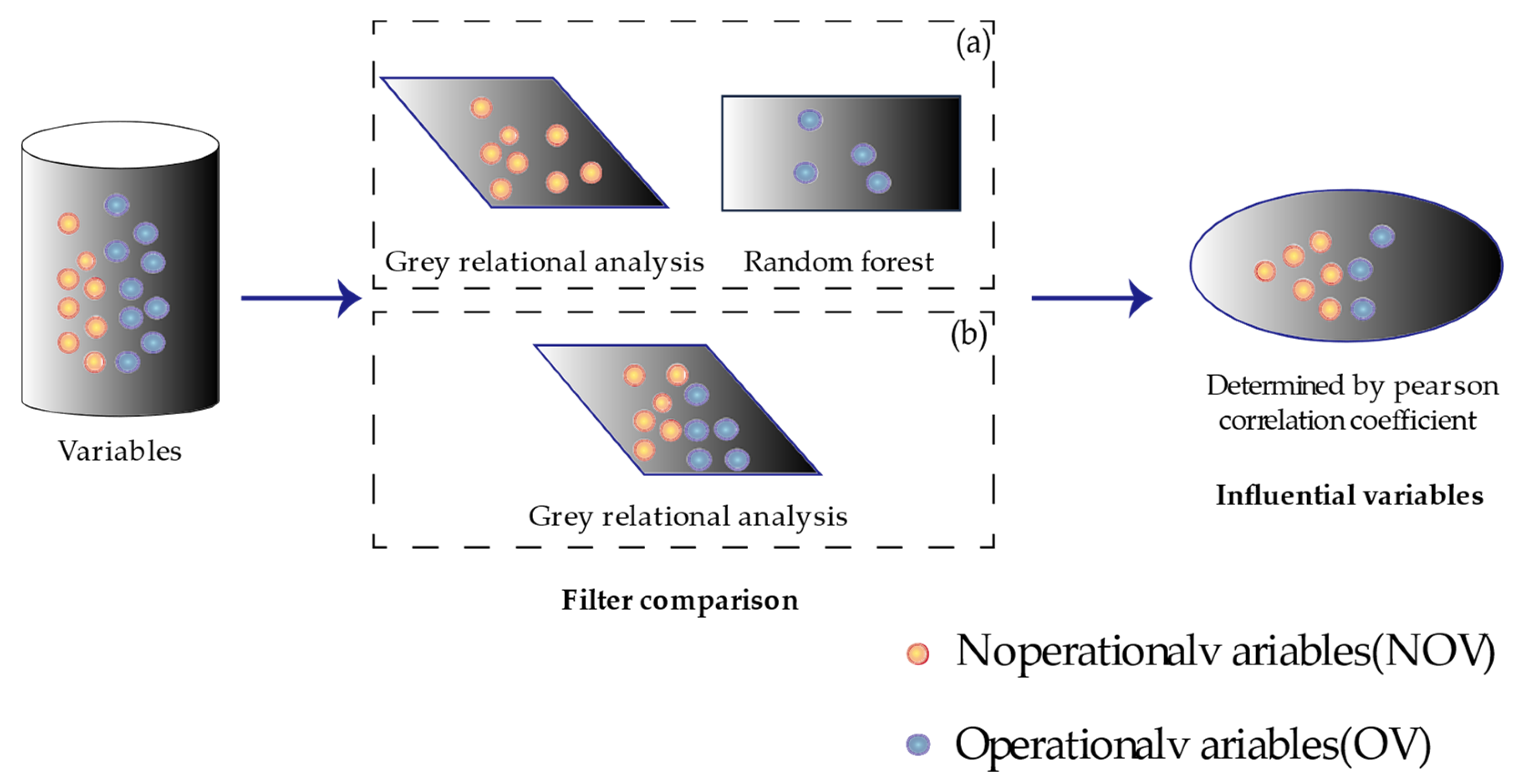
Figure 1. Schematic representation of two variable filtering methods, where the orange and blue spheres represent operational and non-operational variables, respectively. The upper rectangular box (a) represents the hybrid filtering method, and the lower rectangular box (b) shows the method using data filtered only by grey correlation analysis.
Sustainability 15 06571 g001
Figure 2. The topology diagrams of RBF (a) and BP (b) neural networks. Through the network connection, the output and input layers are connected in series to realize the mapping effect from the input layer to the output layer.
Sustainability 15 06571 g002
Figure 3. Flowchart of four different optimization methods for octane number models.
Sustainability 15 06571 g003
Figure 4. Results of non-operational variables that are highly correlated with product RON filtered by the random forest method, and the results were expressed as percentages.
Sustainability 15 06571 g004
Figure 5. Pearson coefficient diagram filtered by two methods introduced in Figure 1a,b. Coefficients near 1 indicate a higher level of correlation. (a,b) corresponding to the results of the hybrid filtering method and grey correlation analysis, respectively. The closer the color to red, the stronger the correlation between the objective and the variables.
Sustainability 15 06571 g005
Figure 6. Comparison results of four prediction methods. Comparison results of four prediction methods. (ad) are the prediction curves of RBF, BP, SVR and XGBoost, respectively. The blue points are all the data points, the red line is fitted by the blue points using the least square method, and the dotted line is the 100% prediction line (that is, the true value = predicted value, i.e., y = x). The greater the overlap between the red line and the dotted line, the more accurate the prediction.
Sustainability 15 06571 g006
Figure 7. Comparison of the results of the four optimization algorithms. (a) is the comparison of optimized values, (b) is the comparison of the stability of the optimized data.
Sustainability 15 06571 g007
Figure 8. Change of RON before and after optimization by SSA. The arrows show the path of the optimization change. The yellow bar chart represents the octane number of the raw materials, while the orange and blue bars represent the octane number of the products before and after optimization by SSA, respectively.
Sustainability 15 06571 g008
Table 1. Part of the data after abnormal and missing processing while the data dimension m is 325 and the sample size n is 326.
pRONSC(µg/g)rRONSaturated Hydrocarbon(v%)S-ZORB.FT_1504.DACA.PVS-ZORB.FT_1504.TOTALIZERA.PVS-ZORB.PC_1001A.PV
189.22188.0090.6053.231840.1439,608,7570.35
289.32169.0090.5052.301641.7339,389,2990.35
389.32177.0090.7052.301600.6839,312,616.50.35
32488.05271.4389.4047.19−10,846.1693,676.8−119.53
32588.12266.0089.4046.72−12,373.3569,836.8−120.05
32688.65266.0089.9046.72−13,900.5445,996.8−120.56
Table 2. Variable filtered by the grey correlation degree method.
Reference
Designator
Variable TypesRelevancyReference DesignatorVariable TypesRelevancy
pRONNOV0.894S-ZORB.TE_1105.PVOV0.768
S-ZORB.FT_9403.PVOV0.796S-ZORB.TE_5006.DACAOV0.767
S-ZORB.LC_1201.PVOV0.789S-ZORB.TE_1601.PVOV0.766
S-ZORB.FC_1203.PVOV0.784S-ZORB.TE_5002.DACAOV0.762
S-ZORB.FC_1201.PVOV0.783S-ZORB.FT_1003.PVOV0.762
S-ZORB.TE_2603.DACAOV0.778S-ZORB.TE_5003.DACAOV0.761
S-ZORB.FC_5202.PVOV0.775S-ZORB.PT_9401.PVOV0.760
S-ZORB.FT_2433.DACAOV0.774S-ZORB.FC_1005.PVOV0.760
S-ZORB.TC_3102.DACAOV0.768Bromine valueNOV0.759
S-ZORB.TE_1105.PVOV0.768S-ZORB.TE_5004.DACAOV0.759
S-ZORB.TE_5006.DACAOV0.767///
Table 3. Variables filtered by method (a), with 4 operational variables and 15 non-operational variables.
Reference DesignatorMinimumMaximumVariable Types
SC (µg/g)57.0392.0NOV
pRON87.291.7NOV
Saturated hydrocarbon (v%)43.263.4NOV
Olefins (v%)14.634.7NOV
S-ZORB.LC_1201.PV49.3850.29OV
S-ZORB.LC_1202.PV49.7050.86OV
S-ZORB.LT_1501.DACA−1.265−1.248OV
S-ZORB.TE_2005.PV412.26428.20OV
S-ZORB.PT_9403.PV0.98660.9985OV
S-ZORB.TE_2004.DACA411.85427.67OV
S-ZORB.RXL_0001.AUXCALCA.PV92.0897.30OV
S-ZORB.TE_2003.DACA411.85427.67OV
S-ZORB.TE_2002.DACA413.08429.49OV
S-ZORB.TE_1604.DACA407.04421.58OV
S-ZORB.TE_1102.DACA417.53432.74OV
S-ZORB.TE_1602.DACA404.67417.88OV
S-ZORB.TC_1606.PV403.25416.71OV
S-ZORB.TE_2103.PV415.82431.20OV
S-ZORB.TE_1603.DACA403.39419.55OV
Table 4. Performance results of the four prediction models, including test and training set performance, evaluated by RMSE and R2.
MethodData PartitionRMSER2
BPTraining set0.05660.9645
Testing set0.33210.9221
RBFTraining set0.06310.8911
Testing set0.84570.7039
XGboostTraining set0.01920.9996
Testing set0.21750.9475
SVRTraining set0.09730.9898
Testing set0.25340.9390
Table 5. List of key parameters defined in four prediction models.
ModelParameter NameParameter ValueModelParameter NameParameter Value
XGboostBase learnerDecision TreeRBFInput layer elements19
Number of base learners M75Hide Layer elements227
Learning Rate η0.1Output layer elements1
L1 Regular Terms λ0Expansion speed of RBF100
L2 Regular Terms γ1BPInput layer elements19
Maximum depth of tree10Hide Layer elements10
SVRLoss-function P0.1Output layer elements1
Kernel function typeRBFTraining algorithmLevenberg-Marquardt
Penalty factor4Learn Rate0.01
Radial basis function parameters0.8MERT0.00001
Disclaimer/Publisher’s Note: The statements, opinions and data contained in all publications are solely those of the individual author(s) and contributor(s) and not of MDPI and/or the editor(s). MDPI and/or the editor(s) disclaim responsibility for any injury to people or property resulting from any ideas, methods, instructions or products referred to in the content.