Flume Experiments and Numerical Simulation of a Barge Collision with a Bridge Pier Based on Fluid–Structure Interaction

Abstract

Bridges across waterways are susceptible to failure from ship collisions. Therefore, to provide a reference for bridge design and protection, reported here is a study of the response of a bridge pier during a collision with a barge. First, sphere–cylinder collision experiments were conducted in a water flume, and the fluid–structure interaction (FSI) method was implemented in the LS-DYNA software to simulate the collision process. The numerical and experimental values of the peak impact force agreed within 10%, thereby validating the FSI method for simulating the sphere–cylinder collision. Next, the FSI method was used to simulate the barge–pier collision process, in which the effects of barge mass, speed, collision angle, and location were considered. The simulated collision results of impact force, crush depth of barge bow, and displacement are summarized and discussed in detail. Unlike the constant added mass (CAM) method, the FSI method considers fluid–structure coupling and reproduces the collision phenomena whereby the barge stops upon collision and then goes into reverse. The water then propels the barge forward to collide with the pier repeatedly. Therefore, the FSI method is more effective for simulating barge–pier collisions.

1. Introduction

Bridges, as vital transportation hubs, are frequently threatened by hazards when there is much traffic; barge collisions are a significant unintentional load. There have been many accidents where ships have crashed into bridge piers and girders, causing bridges to collapse and killing people traveling on the bridge. In addition, the collision can have a serious impact on the sustainability of bridge and lead to a prolonged interruption of traffic on the bridge [1].

Barge–pier collision accidents are happening more frequently all over the globe [2,3]. Eight people were killed in a 2007 collision between a completely loaded sand barge and a pier of the Jiujiang Bridge in China, which led to the collapse of three piers [4]. Two staff members were killed and local traffic was disrupted in 2016 when a ship hotel with 180 guests collided with a bridge over the Main Danube Canal in Germany [5].

Numerous scientists have investigated the theory of ship–bridge collisions and conducted numerical collision analysis due to the high risk and severe repercussions of ship–bridge collisions. When ships are engaged in typical collision and grounding events, Spyros [6] present a technique that simulates the impact of strongly coupled fluid–structure interaction (FSI) effects on the dynamic response of the ships. The role of hydrodynamic restoring pressures is crucial. In order to develop a more accurate model of the impact of a barge on a wooden pier, Wang [7,8] used the finite element (FE) technique. Wang also suggested a novel approach that provides numerical results with acceptable accuracy. After performing a refined analysis using lab tests and numerical simulation, Hao [9] obtained numerical prediction results without considering FSI. Based on the AASHTO (American Association of Highway and Transportation Officials) model, Peng [10] obtained a time-sensitive dynamic prediction of the risk of barge collision using the FE technique. Sha [11] investigated the impact process and damage of a sand barge colliding with a single pier using the FE technique and taking material nonlinearity into account. Yuan [12] suggested a manual calculation method that considered the geometry of the bridge and piers, barge interaction, and impact duration compared to the AASTHO [13] recommendations. In order to demonstrate that the system dramatically lowers the peak impact force and lessens the severity of bridge damage, Jiang [14] introduced a floating steel fender system for protecting bridge piers and verified the numerical model with test results. In order to avoid discretizing the body and to use quick Cartesian grid solvers, immersed boundaries [15,16,17] are used to solve the fluid–solid interaction issue. On the other hand, the immersed formulations do not demand body-fitted discretization, avoiding the frequent grid regeneration that could otherwise be necessary for models requiring significant deformations and displacements.

The researchers above looked into the mechanism and process of barge-bridge collisions, assessed the effects of influencing factors using FE simulations, and investigated facilities and preventative measures for collisions that minimize bridge damage. Many scholars created FE models using the constant added mass (CAM) method, equating the water crashing to 3% to 7% of the barge’s mass. For a more accurate conclusion than the CAM method, the FSI method specifically considered the influence of the water, barge, and pier. However, because doing so takes a lot of time and processing power, only a few researchers have combined experiments with numerical simulations based on the FSI method [18]. Hence, a barge–pier collision FSI approach is urgently required to provide practical designs for various circumstances and improve the bridge sustainability such as decreasing the whole life costs, improving the level of operational capability.

In the study reported here, the barge–bridge collision process was simulated using an ALE algorithm, and flume experiments were conducted to validate the approach’s logic. The barge–bridge FE was developed and tested using LS-DYNA software. The barge’s bulk, speed, impact angle, and location were all considered when creating the simulation.

2. Collision Experiments in Flume

Several models were built for flume tests to examine the impact mechanism and loading of a barge crashing with a bridge pier without fenders. In the experimental channel of Southwest Jiaotong University, sphere collision experiments were carried out to model a barge collision with a bridge pier [19]. The entire experimental procedure was also simulated in LS-DYNA based on the ALE approach. The relevant collision simulation parameters were appropriate when compared to the experimental data. The pertinent information about the sphere collision experiments is described in the following subsections.

2.1. Experiment Model and Devices

In the experiment, there is a hollow sphere as the impactor, a bridge specimen, some measuring transducers, and a fixed steel frame.

Scaled replicas of the barge and the bridge pier were used in the experimental flume to imitate them by the third similitude theorem [20,21]. The material for the sphere and the pier were then taken into consideration. Since it has strong mechanical properties, polymethyl methacrylate (PMMA) is frequently used in model experiments, such as impact model tests [22]. PMMA has tensile and bending strengths between 50 and 70 MPa and 90 and 130 MPa, respectively, with a density between 1150 and 1190 kg/m³ [23]. Due to its lightweight and excellent rigidity, PMMA was chosen for the sphere and pier in the current flume trials.

As seen in Figure 1a, the impactor was built as a hollow sphere with a diameter of 250 mm, while the pier model was built as a hollow cylinder with a diameter of 300 mm and a height of 600 mm. The force-measuring balance fastened to the top end of the pier model and coupled to a stable steel frame served as the principal piece of apparatus in these experiments to measure the horizontal and longitudinal loads (see Figure 1b). An acoustic doppler velocimetry (ADV) was put in the steel frame to measure the water speed (see Figure 1b). The entire experiment was conducted in a flume with the following measurements: 5 m, 2 m, 1.8 m, reinforced glass side walls, and a wide, clear viewing area. Cartesian coordinates are utilized in the following, as indicated in Figure 2, where X represents the flume’s width, Y represents the longitudinal path from the circular cylinder to the hollow sphere, and Z represents the vertical (positive in the upward direction) direction [24]. The sphere was placed 3 m away from the pier model first; then, water was poured into the flume until it was halfway up the pier model.

Based on the ADV’s monitoring during the experiment, the water velocity in the flume was initially permitted to establish a stable condition. After being set free from its resting position, the hollow sphere sped to match the speed of the water before striking the bridge specimen. In order to rule out undesirable situations such as the impactor’s orientation being off or its speed not being adequate, we conducted multiple trials for the same scenario. The tests examined nine situations with various sphere masses and water velocities, all listed in

Table 1. Experimental cases with different sphere masses and water speeds.

Case	Sphere Mass (kg)	Water Speed (m/s)
1	0.65	0.2
2	0.65	0.3
3	0.65	0.4
4	1.00	0.2
5	1.00	0.3
6	1.00	0.4
7	2.00	0.2
8	2.00	0.3
9	2.00	0.4

.

2.2. FE Simulation

The LS-DYNA software created the FE model to simulate sphere collision experiments regarding impactor mass and impact speed. This FE model used the FSI algorithm as a coupling method with the multi-material ALE (Arbitrary Lagrangian–Eulerian) formulation [25]. The bridge–pier cylinder specimen, the air and water fields, two boundaries, and a hollow sphere were all components of the FE model for sphere collision, as shown in Figure 2. While the components of the air and water fields were solid, the hollow sphere and circular cylinder were shell components. Trial calculations led to the mesh sizes for the hollow sphere, circular cylinder, and air and water fields being determined to be 10 mm, 30 mm, and 50 mm, respectively. The contact keyword *CONTACT AUTOMATIC SURFACE TO SURFACE (CASTS) [26] was used between the hollow sphere and the circular cylinder. This article will use the term “failure” to refer to failure to complete a task. The ALE keyword *CONSTRAINED LAGRANGE IN SOLID [27] was used as a motion description technique between fields and structures. The displacements of the bottom nodes of the cylinder were constrained with PFAC = 0.1 to simulate the actual situation. In order to create an initial environment, the keywords *INITIAL HYDROSTATIC ALE and *INITIAL VOLUME FRACTION GEOMETRY were also used.

The keywords *EOS LINEAR POLYNOMIAL and *MAT_ Null were also used (see

Table 2. Material parameters (air).

Material	$\mathit{\rho }$ (kg/m3)	${\mathit{C}}_0,{\mathit{C}}_1,{\mathit{C}}_2,{\mathit{C}}_3,{\mathit{C}}_6$	${\mathit{C}}_4,{\mathit{C}}_5$	${\mathit{E}}_0$ (Pa)
Air	1.293	0	0.400	2.5 × 105

and Equations (1)–(4) for the air). Additionally, the keywords *MAT Null and *EOS GRUNEISEN were applied to the water (

Table 3. Material parameters (water).

Material	$\mathit{\rho }$ (kg/m3)	$\mathit{C}$	${\mathit{S}}_1$	${\mathit{S}}_2$	${\mathit{S}}_3$
Water	1000	1450	1.921	−0.096	0

and Equation (5), the water-specific Gruneisen equation). The sphere impactor and bridge specimen’s linear elasticity were modeled using the keyword* MAT ELASTIC for the models’ material properties (see

Table 4. Material parameters (sphere impactor and bridge specimen).

Material	$\mathit{\rho }$ (kg/m3)	$\mathit{E}$ (Pa)	$\mathit{\nu }$
Sphere impactor	1718.3	3.15 × 109	0.35
Bridge specimen	1190.0	3.15 × 109	0.35

):

$$P=C_0+C_1\mu +C_2{\mu }^2+C_3{\mu }^3+\left(C_4+C_5\mu +C_6{\mu }^2\right)E_0$$

(1)

$$\mu =\frac{\rho }{{\rho }_0}-1$$

(2)

Note that the air is supposed as an ideal gas and some parameters can be set:

$$C_0=C_1=C_2=C_3=C_6=0$$

(3)

$$C_4=C_5=\gamma -1$$

(4)

$$P=\frac{{\rho }_0{C}^2\mu \left[1+\left(1-\frac{{\gamma }_0}{2}\right)\mu -\frac{\alpha }{2}{\mu }^2\right]}{1-\left(S_1-1\right)\mu -S_2\frac{{\mu }^2}{\mu +1}-S_3\frac{{\mu }^3}{{\left(\mu +1\right)}^2}}$$

(5)

2.3. Comparison and Verification

The simulation and experimental results for the nine cases are compared in Figure 3, and the values of the maximum total impact force are listed in

Table 5. Comparison of maximum total impact force between experiments and simulations.

Case	Experiment (N)	Simulation (N)	Relative Error (%)
1	7.224	6.962	3.627
2	7.724	7.312	5.334
3	8.446	8.959	−6.074
4	8.956	8.508	5.002
5	10.552	9.813	7.003
6	12.027	12.335	−2.561
7	10.218	10.542	−3.171
8	12.461	11.434	8.242
9	13.578	13.319	1.907

Note: the relative error R was calculated as $R=\frac{T-S}{T}\times 100\%$, where T is the experimental value and S is the simulation value.

. The component of the impact force in the Y direction, $F_y$, is the combined impact of the sphere and water on the cylinder, while that in the X direction, $F_x$, is generated from the lateral pressure of the flow around the cylinder.

In both the simulation and the experimental data, as shown in Figure 3, a dramatic increase in force was seen during the sphere impact. Nevertheless, the peak’s length was brief, and the force quickly declined. Due to the contact and separation between the sphere and cylinder, this impact induced a sharp change. The water flow force causes future collisions to cause repeated increases and declines in collision force after the initial peak force. Moreover, the FSI-based simulation method replicated these numerous collision occurrences. Figure 3 also shows that the impact results were influenced significantly by the sphere mass and water velocity; with increases in both, $F_y$ increased while $F_x$ decreased.

The comparison of the simulation and experimental data in Figure 3 and Table 5 demonstrate accuracy with a low error rate. The simulation of the sphere colliding with the cylinder is feasible based on the ALE method and LS-DYNA keywords. It may be expanded to a larger-scale simulation of the barge–pier collision because the variations in peak force between simulation and experimental data are within 10% [28].

3. Simulation of Barge–Pier Collision

Further case simulations were conducted using the validated numerical technique to explore pier effects with various parameters, such as barge mass, velocity, barge impact angle, and barge impact site. The impact force, barge crush depth, and pier displacement were studied using numerical models.

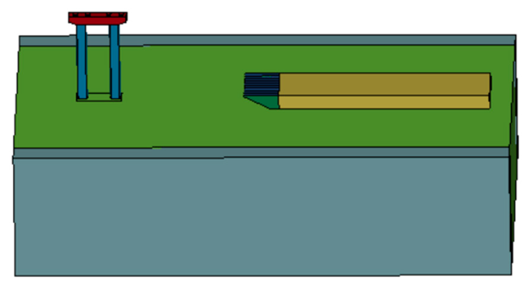
3.1. Barge–Pier Collision Model

The study context used here was a busy navigation channel close to inland waterways to model a barge–pier collision in the field. In this work, a pier with the proportions depicted in Figure 4 was taken into consideration, and the matching FE pier was modeled using 23,728 eight-node solid elements, as depicted in Figure 5. Four comparable blocks, a pier cap, two piers, two pile caps, and four piles comprised the pier. Similar blocks with limitations were placed on top of the pier cap to replicate the superstructure bridge mass. The double piers were topped with a pier cap that had the measurements 14 m by 2.6 m by 1.9 m, as illustrated in Figure 4. As piles connecting the pile tops, four circular piles with a diameter of 1.7 m and a height of 30.2 m were cast in Figure 4. The water rose 32.8 m above the bridge’s foundation in the area nearby. The bridge pier was believed to be fixed in all directions at the beginning of the study [29,30].

The simulations employ the popular JH barge model advised by AASHTO [13]; the JH barge’s relevant parameters are provided in Figure 6 left and

Table 6. Barge dimensions used in the present model.

Symbols	AASHTO 1991 (ft)	This Study (m)
$L_B$	195	59.4
$B_M$	35	10.8
$R_L$	20	8.4
$D_B$	13	4.0
$D_V$	12	3.8
$H_L$	2–3	0.6

. Moreover, LS-DYNA develops an FE barge model (see Figure 6 right). The bow portion and the barge hull behind the bow make up the barge model. Internal trusses and an exterior plate are present in the bow component and are intended to prevent material failures, deformations, and buckling in the bow portion [26]. A 200 mm numerical grid size is chosen for the bow portion based on trial calculations to assure calculation accuracy. The ship’s hull beyond the bow is depicted using a rough mesh because it is not immediately affected by the impact and is not bent, as seen in Figure 6 right. In order to duplicate the bending properties of the inside trusses and outside bow plates, the bow section with deformation is separated into 5921 shell components. There are 19,440 solid components that make up the hull portion. The water field is 120 m long, 50 m broad, and 32.8 m deep, as illustrated in Figure 7. The barge is 30 m in longitude from the bridge pier. In the same direction as the barge, the water is moving at 2 m/s. The water and air were modeled using the multi-material ALE technique, with 61,440 ALE elements in total.

The brittle-damage model *MAT BRITTLE DAMAGE [31], which considers steel and concrete, is used to represent the pier. It allows for the gradual deterioration of shear and tensile strengths along smeared cracks that began under tensile loadings. This model is helpful in impact simulations because it was created primarily to assess brittle concrete damage [32]. According to Table 6, the pier’s related specifications are based on reinforced concrete, where E is Young’s modulus, ν is Poisson’s ratio, and $\sigma$ is the yield stress. The Cowper–Symonds constants of C = 40 s⁻¹ [33] and P = 5 [34] are considered to simulate the effect of the strain rate. By altering the pier cap’s mass density, the bridge superstructure’s influence can be taken into account. The elastic–plastic model *MAT PLASTIC KINEMATIC is used to represent the bow portion because it allows for careful consideration of the isotropic and kinematic hardening plasticity and strain-rate effect [35] provided by Equation (6):

$$\frac{{\sigma }_y}{{\sigma }_s}=1+{\left(\frac{\dot{\epsilon }}{C}\right)}^{1/P}$$

(6)

Furthermore, because the hull component does not clash with the pier, it is modeled using the keyword *MAT ELASTIC.

Table 7. Material properties used in FE simulations.

Material	Input Parameter	Magnitude
Reinforced Concrete	concrete 𝜌	2500 kg/m3
	E	29.58 GPa
	𝜈	0.200
	FRA_RF	0.006
	steel 𝜌	7850 kg/m3
Barge bow	E	210 GPa
	$\nu$	0.270
	𝜎	310 GPa
	C	40
	P	5
Barge hull	$\nu$	0.270
	E	210 GPa

lists the characteristics of these two materials.

The FE model’s contact keyword CASTS was utilized during the collision process between the barge’s bow and the pier, with a dynamic and static friction coefficient of 0.2. With a dynamic and static friction coefficient of 0.3 [7], deformations may occur during the secondary contacts following the collision, which is why the contact term *CONTACT SINGLE SURFACE was utilized in the internal trusses. The contact keyword *CONTACT TIED SURFACE TO SURFACE was also used to connect each component of the pier in the current FE pier model.

3.2. Collision Results with Different Barge Masses

In LS-DYNA, the appropriate FE models were created to study the impact of the barge mass. Studying loading scenarios with barge masses of 500 tons, 750 tons, and 1000 tons involved changing the barge density. After being freed from rest, the barge traveled 3 m/s using the FSI algorithm before colliding with the bridge pier. Based on the barge’s speed and the distance between the pier and the barge, it should be noted that the collision happened at 20 s. In Figure 8, the simulation results for collisions between barges and piers of various masses are contrasted. Figure 9 shows an interval distance between the pier and the barge, where the negative value denotes collision seconds between the two, and the positive number shows their separation.

There are three overall collisions, comprising the first collision and subsequent collisions with various barge masses under the influence of water, as illustrated in Figure 8a. According to Figure 8b, the barge–first pier’s collision with the three distinct masses resulted in peak impact forces of 4.54 MN (20.10 s), 5.19 MN (20.35 s), and 5.56 MN (20.37 s). The outer plates colliding with the pier caused the impact force in the initial collision to increase quickly. The impact force decreases when the outer plates sag. The barge’s interior trusses then run into the pier at the bow. Ultimately, the barge separates from the pier and slows down, bringing the impact force to zero. The phenomenon shows that the barge moves away following the initial impact. This circumstance may be shown in Figure 9, where the positive distance denotes separation, and the negative distance denotes collision. For instance, Figure 10 illustrates the Von Mises stress of the 500-ton barge at 20.4 s, 22.2 s, and 32.9 s, illustrating the first collision, second collision, and separation situations. The phenomenon of secondary collision can be seen in the time series of impact force caused by the barge rocking and internal tissue deforming again, with peak impact forces of 1.25 MN (22.25 s), 1.75 MN (22.63 s), and 1.98 MN (22.75 s), respectively. This is due to the realistic reconstruction of the collision process via the FSI method, as shown in Figure 8a. Because water needs more time to propel bigger barges, the period between the initial collision and the following collisions with three distinct masses increases. The peak impact force and initial contact time rise with increasing barge mass.

The barge crush depth rises sharply to its peak, as depicted in Figure 11a, after which it will expand steadily. It should be noted that barge crush depth refers to the depth at which the barge bow pierces the pier. Before reaching its maximum value during the collision phase, the crush depth initially rises quickly and then falls slightly. The barge is isolated from the pier. Therefore, the depth drops quickly. The barge crush depth keeps rising until it reaches its maximum value as the barge is carried along by the water hitting the pier repeatedly. The maximum crush depth of the barge bow significantly rises with increasing barge mass, with values of 0.40 m, 0.89 m, and 1.38 m. Additionally, as shown in Figure 11b, the maximum displacements of the pier are 0.37, 0.62, and 0.90 m, respectively, illustrating a gradually increasing pattern. Because the barge accelerates the water surrounding the pier, the initial displacement is caused by the impact of water. In general, the mass of the barge can raise the collision index value. Because of the water movement, which results in several collisions between the barge and the pier, barge mass raises the index value of multiple collisions.

3.3. Collision Results with Different Barge Speeds

The barge speed was set to 3 m/s, 4 m/s, and 5 m/s with a mass of 500 tons, giving rise to barge–pier first-contact times of 20 s, 17.5 s, and 16 s, respectively, as shown in Figure 12a. The time coordinate shifts to 15 s to cope with the changes in collision time. The simulation results for barge–pier collisions with different barge speeds are summarized in Figure 12 and Figure 13.

As shown in Figure 12a, there are three overall collisions, including the first collision and subsequent collisions with different barge speeds under the action of water. As shown in Figure 12b, with barge speeds of 3 m/s, 4 m/s, and 5 m/s, the peak impact forces in the barge–pier collision is 4.54 MN (20.10 s), 4.91 MN (17.51 s), and 5.89 MN (16.28 s), respectively. The change in the value of the impact force curve is due to outer plates and internal trusses, as mentioned above. Clearly, as seen in Figure 12a, when increasing the barge speed from 3 m/s to 5 m/s, the phenomenon of secondary collision can be observed in the time series of impact force, with peak impact forces of 1.25 MN (22.25 s), 1.94 MN (21.34 s), and 2.78 MN (20.64 s). It is clear that the time interval between the first collision and the subsequent collision with three different speeds increases because water needs more time to consume the kinetic energy.

According to Figure 13a, the maximum barge crush depths for three barges traveling at three different speeds are 0.40 m, 0.55 m, and 0.66 m, respectively. When barge speed increases, the barge crush depth rises roughly linearly. Because the barge and the pier are separated before reaching the maximum value, the barge crush depth decreases marginally. Additionally, as the speed increases to 3 m/s, 4 m/s, and 5 m/s, the duration of the procedure shortens. Figure 13b displays the simulation outcomes for the displacement of the pier at various speeds. Following the barge’s collision with the pier, the displacement is altered. The maximum pier displacements are 0.37 m, 0.39 m, and 0.34 m for barge speeds of 3 m/s, 4 m/s, and 5 m/s, respectively. These findings suggest that the peak impact force and crush depth are more sensitive to barge speed changes than the pier bending moment and displacement.

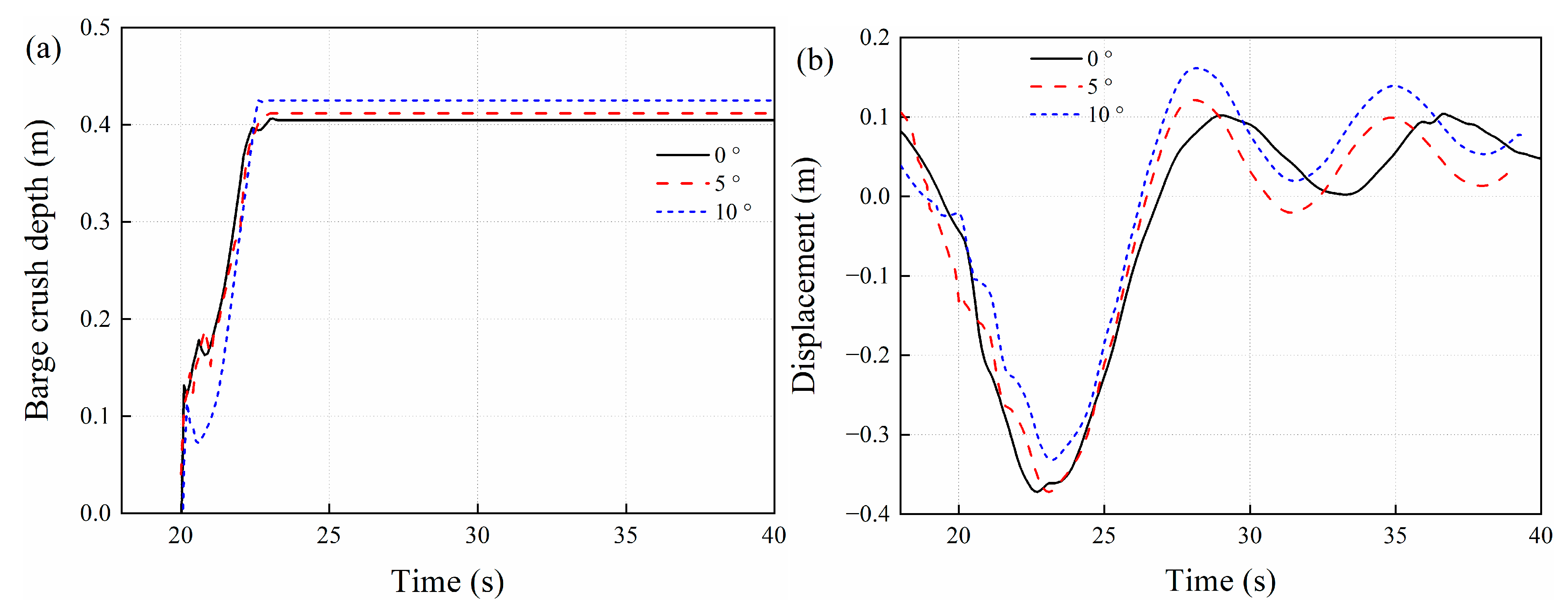
3.4. Collision Results with Different Barge Angles

In a barge–pier collision, the impact angle plays a significant role [36]. The angle formed by the water direction and barge route is known as the collision angle. The simulation results displayed in Figure 14 and Figure 15 correspond to collision angles of 0°, 5°, and 10°, which are used to study its impact. Additionally, 0°, 5°, and 10° denote the angle between the barge and the water.

The impact force time series at the various angles develop similarly, as illustrated in Figure 14a. As depicted in Figure 14b, the peak impact forces are 4.54 MN (20.10 s), 3.78 MN (20.14 s), and 3.75 MN (20.21 s), respectively, at 0°, 5°, and 10°, demonstrating a negative connection. The peak impact force is reduced by 17.6% from 0° to 10° of collision angle. The smaller impact force deforms the outer plates more gradually, causing varying curves in the impact force of 5° and 10°. The phenomena of secondary collision can be seen in the time series of impact force in Figure 14a, with peak impact forces of 1.25 MN (22.25 s), 1.16 MN (22.71 s), and 1.08 MN (23.32 s), respectively. This is due to the realistic reconstruction of the collision process via the FSI approach. Due to the barge’s increased contact area with the water at angles of 0°, 5°, and 10°, raising the collision angle also lengthens the time between the first and second collisions and increases the second impact force.

Concerning the three different impact angles, Figure 15 depicts the barge crush depth and pier displacement evolutions. The maximum barge crush depths of the barge bow in these three distinct scenarios, as shown in Figure 15a, are 0.40 m, 0.41 m, and 0.43 m, respectively. These times series of the barge crush depth indicate an initial quick increase followed by a minor decrease and a steady climb. The maximum pier displacements in these three scenarios are 0.37 m, 0.37 m, and 0.33 m, respectively, as illustrated in Figure 15b. These simulation findings demonstrate that the barge crush depth and pier displacement are mostly unaffected by the collision angle, with comparable evolutions and peaks. In conclusion, the larger the contact angle within the range of 0°–10°, the smaller the peak impact force. However, the depth and displacement of the barge crush are not noticeably impacted by the contact angle.

3.5. Collision Results with Different Collision Locations

Another important factor to take into consideration is the location of the collision on the barge bow. The barges were positioned 0 m, 0.5 m, and 1.0 m off the center line in the simulations. In Figure 16 and Figure 17, the simulation results for these scenarios are displayed.

The impact force time series at the various places develop similarly, as illustrated in Figure 16a. The peak impact forces at 0 m, 0.5 m, and 1 m, respectively, are 4.54 MN (20.10 s), 3.99 MN (20.27 s), and 3.87 MN (20.36 s), as shown in Figure 16b, which illustrates a negative correlation. With peak impact forces of 1.25 MN (22.25 s), 1.14 MN (23.89 s), and 1.05 MN (22.77 s), respectively, the phenomenon of secondary collision can be seen in the time series of impact force, according to the realistic reconstruction of the collision process using the FSI approach in Figure 16a.

As shown in Figure 17, with increasing collision distance from the barge bow’s center, the barge crush depth is 0.40 m, 0.46 m, and 0.55 m, respectively (see Figure 17a). This shows that as the collision position moves farther around the barge bow, the barge crush depth increases; however, the peak impact force of the first collision decreases, the first collision deflects the barge, and the peak force of the second collision is increased. An offset collision leads to more significant barge bow deformation for the collision locations of 0 m, 0.5 m, and 1.0 m. As shown in Figure 17b, the pier displacement is unchanged with the different collision locations.

4. Comparative Analysis of FSI and Added-Mass Methods

The CAM approach, which considers the influence of water speed by adding mass to the barge, is another method frequently used to simulate barge–pier collisions [37]. However, as the barge moves under actual circumstances, the water in the area will either hinder or facilitate the movement, changing the barge’s motion state. In a similar vein, the barge’s response will have an impact on the water in the area, changing its flow state. Compared to the CAM method, the FSI method successfully mimics the interaction between the barge and the water in nature. This section contrasts the FSI and CAM simulations of the barge–pier collision process. A constantly increased mass coefficient of 1.05 was used for the CAM approach to approximate hydrodynamic mass effects [38]. In order to simulate a bridge–pier collision, the barge’s hull is given an addition of 0.05 times the overall mass. At the same time, the remaining variables and material characteristics are left unchanged from those employed in the FSI approach described above. The CAM approach is employed for a collision simulation in two scenarios with a mass of 500 tons and 1000 tons.

We compare the impact force results in Figure 18. Peak impact force values for the initial collision with m = 500 tons and 1000 tons are 4.54 MN (20.10 s) and 5.56 MN (20.37 s) for the FSI approach and 4.59 MN (20.10 s) and 5.84 MN (20.10 s) for the CAM technique, respectively (20.56 s). The impact forces determined by the various calculating techniques are similar in magnitude. It is also shown that FSI and CAM methods can simulate the peak impact force of the first collision. The impact force alone provided by the FSI approach shows numerous peaks after the initial collision, each corresponding to a different collision. The barge bow may constantly be fracturing and failing, so the collision process has evident nonlinear characteristics. The FSI approach could simulate the collision phenomenon whereby:

• Before the collision, the barge is moving in the same direction as the water;
• Upon collision, the barge comes to rest and then goes into reverse;
• The water then propels the barge forward to collide with the pier again.

The FSI cannot be realized using the CAM approach, and the reconstruction of the collision process needs to be more accurate. Hence, the FSI approach works well for modeling barge–pier collisions.

5. Conclusions

In this study, a barge–bridge collision process was simulated using a combination of the FSI and FE methodologies, and the validity of this approach was confirmed using water flume tests. The impact of barge mass, speed, and collision angle and position on the simulation results were considered when creating and analyzing the barge–bridge model in the LS-DYNA program. A comprehensive summary and discussion of the simulation results for the impact force, the barge bow’s crush depth, and pier displacement was conducted. The following conclusions are taken from the findings:

(1)

With relative errors in the peak force of less than 10%, the simulation results and the experiment for sphere–cylinder collisions in the water flume were very consistent. This demonstrated that it was practical and logical to model a sphere colliding with a cylinder using the ALE approach and that this model could be expanded to model a barge–pier collision at a larger size.

(2)

The barge mass and speed considerably affect the dynamic response of the barge–pier collision, according to the general conclusions drawn from the barge–pier crash simulations performed using the FSI method. In contrast, the collision’s angle and position have negligible impacts. With increasing barge mass and speed, all peak values of impact forces, barge crush depth, and pier displacement significantly rose in contrast to fluctuating displacement with different speeds; with increasing collision angle and location offset, peak impact forces substantially dropped, while other index values were only marginally altered in comparison to growing depth with different collision sites.

(3)

The first collision’s maximum impact force could be replicated using the FSI and AM approaches. The FSI approach, in contrast to the CAM method, could replicate the collision phenomenon where (i) the barge moved in the same direction as the water prior to the collision, (ii) stopped after the impact and then reversed, and (iii) the water then forced the barge forward to crash with the pier again. As a result, the FSI approach is a useful tool for modeling barge–pier collisions.

References

1. Abdelkarim, O.I.; ElGawady, M.A. Performance of bridge piers under vehicle collision. Eng. Struct. 2017, 140, 337–352. [Google Scholar] [CrossRef]
2. Lee, G.C.; Mohan, S.; Huang, C.; Fard, B.N. A Study of US Bridge Failures (1980–2012); MCEER: Buffalo, NY, USA, 2013. [Google Scholar]
3. Knott, M.A. Vessel collision design codes and experience in the United States. In Ship Collision Analysis; Routledge: London, UK, 2017; pp. 75–84. [Google Scholar]
4. Knott, M.; Winters, M. Ship and barge collisions with bridges over navigable waterways. In Proceedings of the 34th PIANC World Congress, Panama City, Panama, 7–12 May 2018; pp. 1–16. [Google Scholar]
5. Gluver, H. Ship Collision Analysis. In Proceedings of the International Symposium on Advances in Ship Collision Analysis, Copenhagen, Denmark, 10–13 May 1998; Routledge: London, UK, 2017. [Google Scholar]
6. Sang, J.K.; Krgersaar, M.; Ahmadi, N.; Hirdaris, S. The influence of fluid structure interaction modelling on the dynamic response of ships subject to collision and grounding. Mar. Struct. 2021, 75, 102875. [Google Scholar]
7. Jiang, H.; Wang, J.; Chorzepa, M.G.; Zhao, J. Numerical investigation of progressive collapse of a multispan continuous bridge subjected to vessel collision. J. Bridge Eng. 2017, 22, 04017008. [Google Scholar] [CrossRef] [Green Version]
8. Song, Y.; Wang, J. Development of the impact force time-history for determining the responses of bridges subjected to ship collisions. Ocean Eng. 2019, 187, 106182. [Google Scholar] [CrossRef]
9. Sha, Y.; Hao, H. Laboratory tests and numerical simulations of barge impact on circular reinforced concrete piers. Eng. Struct. 2013, 46, 593–605. [Google Scholar] [CrossRef]
10. Peng, K. Dynamic ship-bridge collision risk decision method based on time-dependent AASHTO model. J. Inst. Eng. Ser. A 2021, 102, 305–313. [Google Scholar] [CrossRef]
11. Sha, Y.; Hao, H. Nonlinear finite element analysis of barge collision with a single bridge pier. Eng. Struct. 2012, 41, 63–76. [Google Scholar] [CrossRef]
12. Yuan, P.; Harik, I.E. Equivalent barge and flotilla impact forces on bridge piers. J. Bridge Eng. 2010, 15, 523–532. [Google Scholar] [CrossRef] [Green Version]
13. AASHTO. Guide Specification and Commentary for Vessel Collision Design of Highway Bridges; American Association of State Highway and Transportation Officials: Washington, DC, USA, 2009. [Google Scholar]
14. Jiang, H.; Chorzepa, M.G. Case study: Evaluation of a floating steel fender system for bridge pier protection against vessel collision. J. Bridge Eng. 2016, 21, 05016008. [Google Scholar] [CrossRef]
15. Karimnejad, S.; Delouei, A.A.; Başağaoğlu, H.; Nazari, M.; Shahmardan, M.; Falcucci, G.; Lauricella, M.; Succi, S. A Review on Contact and Collision Methods for Multi-body Hydrodynamic problems in Complex Flows. Commun. Comput. Phys. 2022, 32, 899–950. [Google Scholar] [CrossRef]
16. Afra, B.; Delouei, A.A.; Mostafavi, M.; Tarokh, A. Fluid-structure interaction for the flexible filament’s propulsion hanging in the free stream. J. Mol. Liq. 2021, 323, 114941. [Google Scholar] [CrossRef]
17. Bhalla, A.P.S.; Bale, R.; Griffith, B.E.; Patankar, N.A. A unified mathematical framework and an adaptive numerical method for fluid–structure interaction with rigid, deforming, and elastic bodies. J. Comput. Phys. 2013, 250, 446–476. [Google Scholar] [CrossRef]
18. Tao, P. Simulation Analysis and Model Experimental Study on Ship-Bridge Collision Force; Nanjing University of CAEronautics and Astronautics: Nanjing, China, 2012. (In Chinese) [Google Scholar]
19. Hong, J.; Wei, K.; Shen, Z.; Xu, B.; Qin, S. Experimental study of breaking wave loads on elevated pile cap with rectangular cross-section. Ocean Eng. 2021, 227, 108878. [Google Scholar] [CrossRef]
20. Yang, Q. Numerical Investigations of Scale Effects on Local Scour around a Bridge Pier; Florida State University: Tallahassee, FL, USA, 2005. [Google Scholar]
21. Tversky, A. Features of similarity. Psychol. Rev. 1977, 84, 327. [Google Scholar] [CrossRef]
22. Ali, U.; Karim, K.J.B.A.; Buang, N.A. A review of the properties and applications of poly (methyl methacrylate)(PMMA). Polym. Rev. 2015, 55, 678–705. [Google Scholar] [CrossRef]
23. Lee, M.; Koo, T.; Lee, S.; Min, B.H.; Kim, J.H. Morphology and physical properties of nanocomposites based on poly (methyl methacrylate)/poly (vinylidene fluoride) blends and multiwalled carbon nanotubes. Polym. Compos. 2015, 36, 1195–1204. [Google Scholar] [CrossRef]
24. Xu, B.; Wei, K.; Qin, S.; Hong, J. Experimental study of wave loads on elevated pile cap of pile group foundation for sea-crossing bridges. Ocean Eng. 2020, 197, 106896. [Google Scholar] [CrossRef]
25. Slavik, T.P. A coupling of empirical explosive blast loads to ALE air domains in LS-DYNA®. IOP Conf. Ser. Mater. Sci. Eng. 2010, 10, 012146. [Google Scholar] [CrossRef] [Green Version]
26. Consolazio, G.R.; Cook, R.A.; Biggs, C.A.E.; Cowan, D.R.; Bollmann, H.T. Barge impact testing of the St. George Island causeway bridge. In Phase II: Design of Instrumentation Systems; Bridge Superstructures; Department of Civil and Coastal Engineering, University of Florida: Gainesville, FL, USA, 2003. [Google Scholar]
27. Ziong, E.C. Finite Element Simulation Study on Circular Concrete Bridge Piers Subjected to Vehicle Collision; Universiti Teknologi Petronas: Seri Iskandar, Malaysia, 2014. [Google Scholar]
28. Zhang, X.; Wang, X.; Chen, W.; Wen, Z.; Li, X. Numerical study of rockfall impact on bridge piers and its effect on the safe operation of high-speed trains. Struct. Infrastruct. Eng. 2020, 17, 1–19. [Google Scholar] [CrossRef]
29. Gholipour, G.; Zhang, C.; Li, M. Effects of soil–pile interaction on the response of bridge pier to barge collision using energy distribution method. Struct. Infrastruct. Eng. 2018, 14, 1520–1534. [Google Scholar] [CrossRef]
30. Rudan, S.; Ćatipović, I.; Berg, R.; Völkner, S.; Prebeg, P. Numerical study on the consequences of different ship collision modelling techniques. Ships Offshore Struct. 2019, 14, 387–400. [Google Scholar] [CrossRef]
31. LSTC. LS-DYNA. In Keyword User’s Manual; Version 971; Livermore Software Technology Corporation: Livermore, CA, USA, 2007. [Google Scholar]
32. Abedini, M.; Zhang, C. Performance Assessment of Concrete and Steel Material Models in LS-DYNA for Enhanced Numerical Simulation, A State of the Art Review. Arch. Comput. Method Eng. 2020, 28, 2921–2942. [Google Scholar] [CrossRef]
33. Cowper, G.R.; Symonds, P.S. Strain-Hardening and Strain-Rate Effects in the Impact Loading of Cantilever Beams; Brown University: Providence, RI, USA, 1957. [Google Scholar]
34. Jones, N. Structural Impact; Cambridge University Press: Cambridge, UK, 2011. [Google Scholar]
35. Fan, W.; Xu, X.; Zhang, Z.; Shao, X. Performance and sensitivity analysis of UHPFRC-strengthened bridge columns subjected to vehicle collisions. Eng. Struc. 2018, 173, 251–268. [Google Scholar] [CrossRef]
36. Pedersen, P.T.; Chen, J.; Zhu, L. Design of bridges against ship collisions. Mar. Struct. 2020, 74, 102810. [Google Scholar] [CrossRef]
37. Förster, C.; Wall, W.A.; Ramm, E. Artificial constant added mass instabilities in sequential staggered coupling of nonlinear structures and incompressible viscous flows. Comput. Method Appl. M 2007, 196, 1278–1293. [Google Scholar] [CrossRef]
38. Kantrales, G.C.; Davidson, M.T.; Consolazio, G.R. Influence of Impact-Induced Relative Motion on Effective Barge Flotilla Mass. J. Bridge Eng. 2019, 24, 04019019. [Google Scholar] [CrossRef]
Figure 1. Experimental setup and instrumentation: (a) the impactor; (b) bridge specimen and testing instruments.
Sustainability 15 06445 g001
Figure 2. Finite element (FE) model of sphere collision experiments.
Sustainability 15 06445 g002
Figure 3. Comparison of components of impact force from simulations and experiments for the nine cases ( F s : impact composite force in simulation; Ft: impact composite force in the experiment).
Sustainability 15 06445 g003aSustainability 15 06445 g003b
Figure 4. Pier configurations (unit: m).
Sustainability 15 06445 g004
Figure 5. Details of FE pier (unit: m): (a) front view; (b) side view.
Sustainability 15 06445 g005
Figure 6. Dimension parameters and element definition of the hopper barge.
Sustainability 15 06445 g006
Figure 7. FE model for barge–pier collision.
Sustainability 15 06445 g007
Figure 8. Time series of (a) overall process and (b) red boxing process of impact force in collisions with different barge masses.
Sustainability 15 06445 g008
Figure 9. Interval distance of the pier and barge.
Sustainability 15 06445 g009
Figure 10. Von Mises stress of the 500-ton barge at different times; (a) time = 20.4 s, (b) time = 22.2 s, and (c) time = 32.9 s.
Sustainability 15 06445 g010
Figure 11. Time series of (a) barge crush depth and (b) pier displacement in collisions with different barge masses.
Sustainability 15 06445 g011
Figure 12. Time series of (a) overall process and (b) red boxing process of impact force in collisions with different barge speeds.
Sustainability 15 06445 g012
Figure 13. Time series of (a) barge crush depth and (b) pier displacement in collisions with different barge speeds.
Sustainability 15 06445 g013
Figure 14. Time series of (a) overall process and (b) red boxing process of impact force in collisions with different barge angles.
Sustainability 15 06445 g014
Figure 15. Time series of (a) barge crush depth and (b) pier displacement in collisions with different barge angles.
Sustainability 15 06445 g015
Figure 16. Time series of (a) overall process and (b) red boxing process of impact force in collisions with different collision locations.
Sustainability 15 06445 g016
Figure 17. Time series of (a) barge crush depth and (b) pier displacement in collisions with different collision locations.
Sustainability 15 06445 g017
Figure 18. Comparison of impact force between fluid–structure interaction (FSI) and constant added mass (CAM) methods.
Sustainability 15 06445 g018