Lithium-Ion Battery Remaining Useful Life Prediction Based on Hybrid Model

Abstract

Accurate prediction of the remaining useful life (RUL) is a key function for ensuring the safety and stability of lithium-ion batteries. To solve the capacity regeneration and model adaptability under different working conditions, a hybrid RUL prediction model based on complete ensemble empirical mode decomposition with adaptive noise (CEEMDAN) and a bi-directional gated recurrent unit (BiGRU) is proposed. CEEMDAN is used to divide the capacity into intrinsic mode functions (IMFs) to reduce the impact of capacity regeneration. In addition, an improved grey wolf optimizer (IGOW) is proposed to maintain the reliability of the BiGRU network. The diversity of the initial population in the GWO algorithm was improved using chaotic tent mapping. An improved control factor and dynamic population weight are adopted to accelerate the convergence speed of the algorithm. Finally, capacity and RUL prediction experiments are conducted to verify the battery prediction performance under different training data and working conditions. The results indicate that the proposed method can achieve an MAE of less than 4% with only 30% of the training set, which is verified using the CALCE and NASA battery data.

1. Introduction

Lithium-ion batteries are widely used in new-energy vehicles, communication equipment, and aerospace electronics owing to their fast-charging rate and long life [1]. However, with the accumulation of cycles, the performance of lithium-ion batteries inevitably deteriorates, leading to system failure and possibly even safety accidents [2,3]. Therefore, it is important to efficiently and accurately predict the Remaining Useful Life (RUL) of Li-ion batteries. During the long-term use of lithium-ion batteries, along with the increasing number of charge and discharge cycles, some irreversible chemical reactions occur inside the battery, resulting in increased internal resistance and performance degradation [4,5,6]. Reliable life prediction techniques not only allow for more efficient use of the battery but also reduce the incidence of failure [7]. RUL is the number of charge and discharge cycles from new to end of life (EOL) under certain operating conditions, with a typical 20% capacity degradation upon reaching EOL [8,9,10].

Currently, life prediction methods for lithium-ion batteries are mainly divided into model and data-driven methods [11,12]. Although the prediction accuracy of lithium-ion batteries based on the model method is high, it depends significantly on the modeling of the internal physical and chemical properties of the battery [13]. The data-driven method can explore the relationship between the external parameters and internal state of the battery without building a complex battery model. Babaeiyazdi et al. [14] designed a model with electrochemical impedance spectroscopy (EIS) and Gaussian process regression (GPR) to predict the state of charge. Ren et al. proposed the use of a convolutional neural network (CNN) and long short-term memory (LSTM) to improve the prediction accuracy of data-driven methods with insufficient degradation data [15]. Zhao et al. combined a broad learning system algorithm and LSTM to increase the size of the training data. The results demonstrated that the training data can be reduced to only 25% using a data-driven method [16]. Yao et al. [17] used particle swarm optimization to optimize (PSO) the parameters of an extreme learning machine (ELM) and effectively predict the RUL of lithium-ion batteries. However, it is difficult to accurately predict battery capacity using a data-driven method owing to the capacity regeneration phenomenon [18,19].

With the aim of tackling the problem of battery capacity regeneration, this study aims to eliminate the influence of regeneration capacity on global prediction. Cheng et al. [20] used Empirical Mode Decomposition (EMD) to decompose the original capacity into a series of intrinsic mode functions from high to low frequencies, thus reducing the impact of capacity regeneration. However, mode aliasing occurs during EMD decomposition, which interferes with the signal decomposition. Chen et al. [21] adopted an integrated empirical mode decomposition to add Gaussian white noise to the original signal to reduce modal mixing. However, EEMD may produce some false components in the process of adding noise to the signal, which affects subsequent signal analysis. CEEMDAN [22] was improved based on EEMD by adding pairs of Gaussian white noise in each decomposition. Averaging was then used to solve the problem of white noise transmission from high frequency to low frequency and to suppress the generation of modal aliasing and false components, which is more suitable for time-frequency analysis of nonlinear and non-stationary signals. The nonlinear and non-stationary characteristics of the battery capacity curve match the application range of the CEEMDAN algorithm [23,24,25]. Therefore, CEEMDAN was selected to extract the signal characteristics of battery capacity.

The judgment accuracy of a neural network depends excessively on the selection of weights and thresholds, which requires a large amount of training data. The operation is complex, and its stability is insufficient. The optimal threshold can easily be changed [26,27]. Ding et al. [28] proposed cuckoo search (CS) optimization to optimize the decomposition layer of variational model decomposition as the input of a gated recurrent unit (GRU). However, the IMF component decomposed by CEEMDAN has different signal frequencies and requirements for universality of neural networks [29]. Therefore, the grey wolf optimization (GWO) algorithm was used to optimize the network parameters and improve the adaptability of the network. The GWO algorithm was proposed by Mirjalili [30], based on the observation of predator hunting in nature. The grey wolf optimization algorithm model is simple and realizable, and its optimization performance in many fields is no less than that of other meta-heuristic swarm intelligence algorithms [31,32,33]. Owing to the shortcomings of the GWO algorithm in large-scale optimization problems, such as premature convergence, easy local optimization, and low convergence accuracy, many researchers have proposed various solutions from different aspects. Nadimi-Shahraki et al. [34] proposed an improved GWO based on dimension-learning-based hunting (DLH) to maintain the diversity of the wolf population. Long et al. [35] proposed a hybrid algorithm using GWO and CS to balance exploration and exploitation. Zhao et al. [36] used chaos-enhanced GWO for the overall search and the initial population of the wolf can be restricted to a certain range. However, this method only considers the diversity of the initial population and ignores the weight and position relationships of different wolf groups.

This study proposed a comprehensive RUL prediction method. First, the original capacity of the battery was decomposed using CEEMDAN to eliminate interference noise with low correlation. IGWO was used to optimize the parameters of the neural network. Finally, CALCE and NASA data were tested to verify the effectiveness and stability of this method. The following were achieved:

(1)

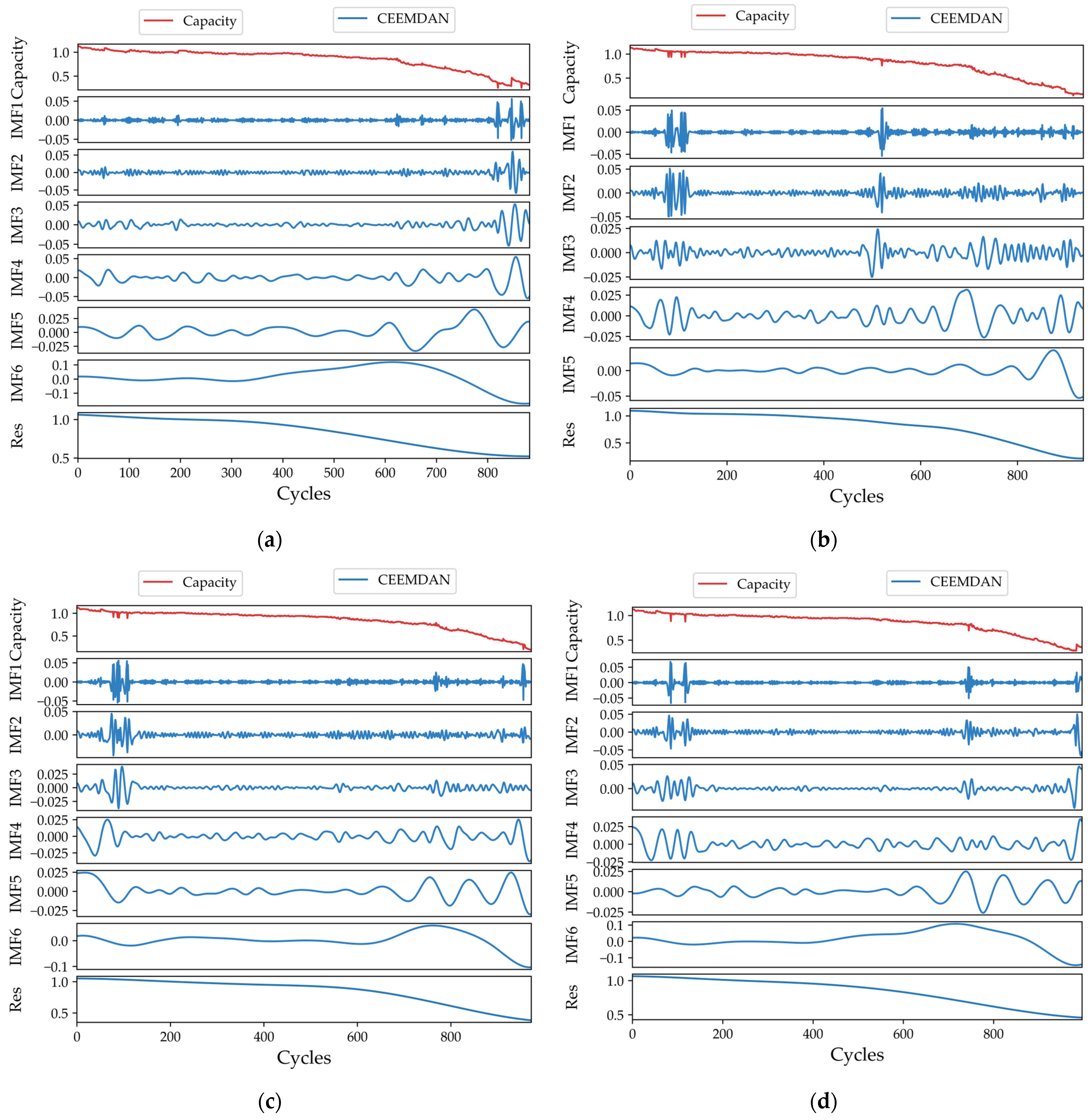
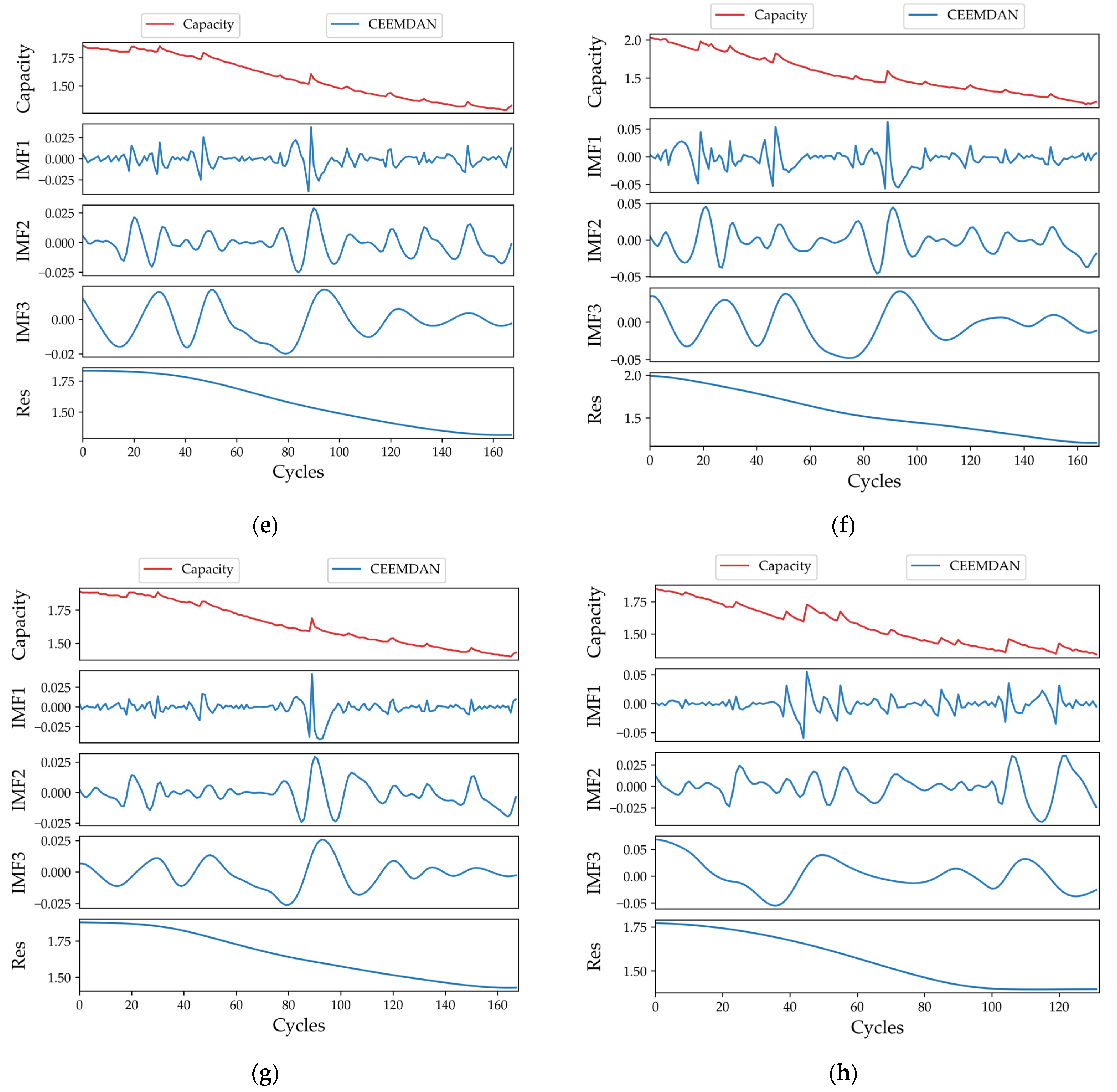
The regeneration of battery capacity was eliminated through CEEMDAN, and the accuracy of the prediction model was improved.

(2)

The weights of the initial population, control factor, and wolf group in the traditional GWO were improved to enhance the diversity and iteration speed of the population.

(3)

IGWO was used to improve the parameters of neurons, dropout rate, batch size, etc. in the neural network. The universality of RUL prediction was improved for IMF components at different frequencies.

2. Methodology

2.1. Battery Remaining Useful Life

The remaining life of a battery represents the number of battery cycles from its rated capacity to the end of its life [37]. The formula is as follows:

$$RUL=N_{eol}-N$$

(1)

where N_eol is the maximum number of battery cycles, and N represents the number of cycles of the battery.

2.2. Complete Ensemble Empirical Mode Decomposition with Adaptive Noise

CEEMDAN is an improved algorithm based on EEMD and EMD. It has the advantages of a good mode spectrum separation effect, fewer shielding iterations, and low calculation cost, and is often used to process non-stationary and nonlinear signals [38,39]. The specific steps of CEEMDAN are as follows:

Step 1: Add Gaussian white noise to the original capacity signal r₀. EMD is used to decompose the new signal to obtain the first IMF component. Then the first residual is calculated according to the following equations:

$$\overline{IM{F}_1}=\frac{1}{I}{\displaystyle \sum _{i=1}^{I}IM{F}_1}$$

(2)

$$r_1=r_0-\overline{IM{F}_1}$$

(3)

Step 2: Add adaptive white noise to the remaining signal of Equation (2) and decompose the second modal component obtained after EMD processing, using:

$$IM{F}_2=\frac{1}{n}{\displaystyle \sum _{i=1}^I{E}_1(r_1+{\epsilon }_1{E}_1({\omega }_i(t)))}$$

(4)

Step 3: Steps 2 and 3 are repeated to decompose the signal and t. The k residual and k+1 modal components are, respectively, as follows:

$$r_k=r_{k-1}-IM{F}_k$$

(5)

$$IM{F}_{k+1}=\frac{1}{I}{\displaystyle \sum _{i=1}^I{E}_1(r_k+{\epsilon }_k{E}_k({\omega }_i(t))})$$

(6)

where n denotes the total number of modal components. The final residual is:

$$r=x-{\displaystyle \sum _{i=1}^I\overline{IMF}}$$

(7)

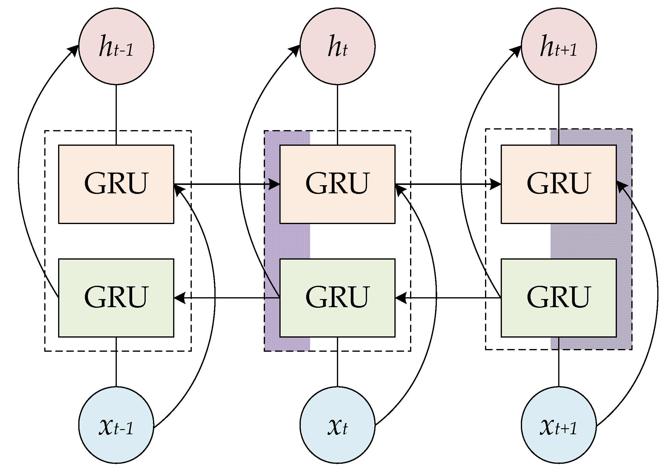
2.3. Bidirectional Gate Recurrent Unit

The remaining life of a battery represents the number of cycles of the battery from its rated capacity to the end of its life. The equation is as follows:

$$r_t=\sigma (W_r\cdot [h_{t-1},x_t])$$

(8)

$$z_t=\sigma (W_z\cdot [h_{t-1},x_t])$$

(9)

$$\widetilde{h_t}=\tan (W_{\widetilde{h_t}}\cdot [r_t\ast h_{t-1},x_t])$$

(10)

$$h_t=(1-z_t)\ast h_{t-1}+z_t\ast {\tilde{h}}_{t-1}$$

(11)

where r_t is the reset gate, z_t is the update gate, x_t denotes the current input, h_t−1 is the last-moment output, $\widetilde{h_t}$ is the current output, σ and tan are the activation functions, W_r and W_z are weight matrices, “·” is the dot product, and “∗” is the matrix product.

The classical GRU structure uses one-way propagation along the sequence transfer direction, and time is only related to the past time [40]. However, in some cases, feedback on the future sequence value at a certain time is considered when building the model. This information can be used to modify a model [41]. Therefore, a BiGRU model was constructed, as shown in Figure 1. The basic concepts are as follows. For each training sequence, two GRU models are established in the forward and reverse directions, and the hidden layer nodes of the two models are connected to the same output layer. This data-processing method can provide complete historical and future information for each time point in the input sequence of the output layer [42]. Therefore, the BiGRU network can learn the relationship between past and future load-influencing factors and the current load, which helps extract the characteristics of capacity data. The output is shown in Equations (12)–(14).

$${\overrightarrow{h}}_t=GRU(x_t,{\overrightarrow{h}}_{t-1})$$

(12)

$${\overleftarrow{h}}_t=GRU(x_t,{\overleftarrow{h}}_{t-1})$$

(13)

$$h_t=w_t{\overrightarrow{h}}_t+v_t\overleftarrow{h}+b_t$$

(14)

where ${\overrightarrow{h}}_t$ is the output of the forward hidden layer at time t; ${\overleftarrow{h}}_t$ is the output of the reverse hidden layer at time t; w_t and v_t, respectively, represent the forward hidden layer state ${\overrightarrow{h}}_t$ corresponding to the two-way GRU at time t and the reverse hidden state ${\overleftarrow{h}}_t$ corresponding weight, respectively; and b_t represents the offset corresponding to the hidden layer state at time t. The structure of the BiGRU is shown in Figure 1.

In the forward layer, the forward direction from time step 1 to time step t is calculated, and the output h of each forward hidden layer is obtained and saved in ${\overrightarrow{h}}_t$. In the reverse layer, a reverse calculation is performed from the current time step t to the previous time step t − 1, and the output h of each reverse hidden layer is obtained and saved in ${\overleftarrow{h}}_t$. Finally, the final output is obtained by combining the output results of the forward and reverse layers.

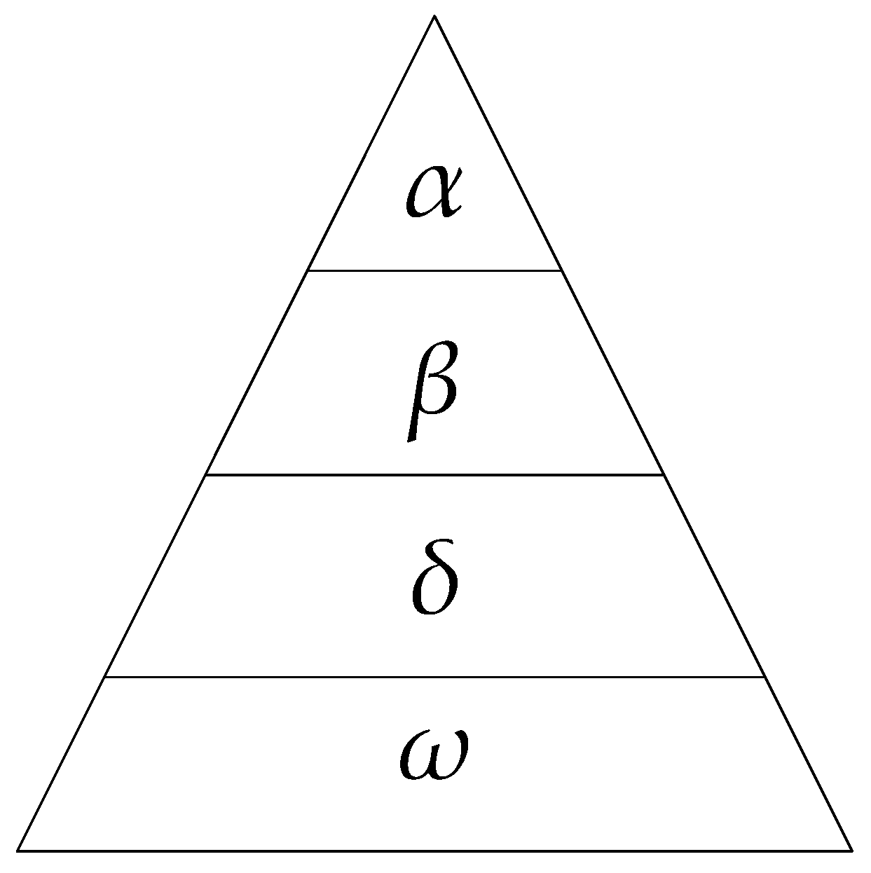
2.4. The Grey Wolf Optimizer

Swarm intelligence is a powerful branch of computational intelligence for solving optimization problems. The SI algorithm simulates and imitates natural social behaviors, such as fish schools, birds, and animals [43]. The GWO algorithm is inspired by the hunting behavior of grey wolves and is considered one of the fastest swarm intelligence algorithms.

In each group of grey wolves, there is a common social class that represents the power and dominance of each wolf, as shown in Figure 2. In the implementation process of the GWO algorithm, grey wolves attack prey based on fitness values and social levels. The main process of grey wolf hunting is to round up and attack [44]. The hunting technology and social level of grey wolves can be used to design mathematical models as follows:

Step 1: Surround the prey. The social class of the grey wolf was modeled and α was adopted as the best solution. The second and third best solutions were β and δ, respectively. The remaining candidate solutions are considered as ω.

$$\overrightarrow{X}={\overrightarrow{X}}_p-\overrightarrow{A}\times \overrightarrow{D}$$

(15)

$$\overrightarrow{D}=\left|\overrightarrow{C}\times {\overrightarrow{X}}_p-\overrightarrow{X}\right|$$

(16)

where D is the distance between the prey and wolf pack, A and C are the coefficient vectors, X_p is the position vector of the prey, X is the position vector of the grey wolf, and n is the current iteration number. Vectors A and C can be calculated separately.

$$\overrightarrow{A}=2\times \overrightarrow{\alpha }\times {\overrightarrow{r}}_1-\overrightarrow{\alpha }$$

(17)

$$\overrightarrow{C}=2\times {\overrightarrow{r}}_2$$

(18)

where r₁ and r₂ are the random vectors of [0, 1]. The parameter a is linear, as shown in Equation (19), and decreases from 2 to 0 during the iterations.

$$\overrightarrow{\alpha }=2\times \left(1-\frac{i}{I}\right)$$

(19)

where I is the maximum number of iterations.

Step 2: Attack prey. The grey wolf can identify and surround this position. It is typically composed of an α guidance. β and δ participated in occasional hunting. However, in the virtual search space, the location of the best prey is unknown. To simulate the hunting behavior of grey wolves mathematically, it was assumed that α was the best candidate solution. β and γ are the potential locations of the prey. Therefore, each grey wolf can be updated according to the best location, as shown in Equations (20)–(22).

$$\left\{\begin{array}{c}\overrightarrow{D_{\alpha }}=\left|\overrightarrow{C_1}\cdot \overrightarrow{X_{\alpha }}\right|-\overrightarrow{X}\\ \overrightarrow{D_{\beta }}=\left|\overrightarrow{C_2}\cdot \overrightarrow{X_{\beta }}\right|-\overrightarrow{X}\\ \overrightarrow{D_{\delta }}=\left|\overrightarrow{C_3}\cdot \overrightarrow{X_{\delta }}\right|-\overrightarrow{X}\end{array}\right.$$

(20)

$$\left\{\begin{array}{c}\overrightarrow{X_1}=\overrightarrow{X_{\alpha }}-\overrightarrow{A_1}\cdot \overrightarrow{D_{\alpha }}\\ \overrightarrow{X_2}=\overrightarrow{X_{\beta }}-\overrightarrow{A_2}\cdot \overrightarrow{D_{\beta }}\\ \overrightarrow{X_3}=\overrightarrow{X_{\delta }}-\overrightarrow{A_3}\cdot \overrightarrow{D_{\delta }}\end{array}\right.$$

(21)

$$\overrightarrow{X}(n+1)=\frac{1}{3}\times ({\overrightarrow{X}}_1+{\overrightarrow{X}}_2+{\overrightarrow{X}}_3)$$

(22)

2.5. Improved Grey Wolf Optimizer

In the GWO, α, β, and δ guide the ω wolf moves in the best direction. This behavior may lead to a locally optimal solution. The distribution of the initial wolves also yields a locally optimal solution for the algorithm. To overcome these problems, an improved grey wolf optimizer (IGWO) is proposed in this section. Improvements include a new search strategy associated with the selection and update steps. IGWO includes four stages: initialization, movement, selection, and update.

2.5.1. Population Initialization

Because the initial grey wolf population determines whether the optimal path can be found and the convergence speed, the diversity of the initial population helps prove the performance of the algorithm in finding the optimal path. The traditional GWO randomly initializes the location of the wolf group, which primarily affects the search efficiency of the algorithm. The initialized population needs to be distributed as evenly as possible in the initial space to improve the diversity of the initial wolf group and to prevent the algorithm from falling into the local optimal solution.

GWO usually generates an initialization population randomly. The more uniformly distributed the initial population in the search space, the better the optimization efficiency and accuracy of the algorithm. To improve population diversity, tent mapping was used to initialize the population. The tent map has a simple structure, uniform density distribution, and good ergodicity. The tent mapping is expressed as:

$$x_t=\left\{\begin{array}{cc}2x& 0\le x_t\le 0.5\\ 2(1-x)& 0.5<x_t\le 1\end{array}\right.$$

(23)

The initial wolf pack was randomly generated within the specified search range, as shown in Equation (24).

$$\begin{array}{cc}{X}_{ij}=L_b+x_t\cdot (U_b-L_b),& i\in [1,N],j\in [1,D]\end{array}$$

(24)

where x_t is a random value in the range [0, 1]; U_b and L_b are the upper and lower bounds of the component, respectively; X_ij is the position of the jth wolf in the ith iteration; N is the number of wolves; and D is the search dimension. The improved chaotic mapping of the wolf position can ensure a uniform distribution of the initial population.

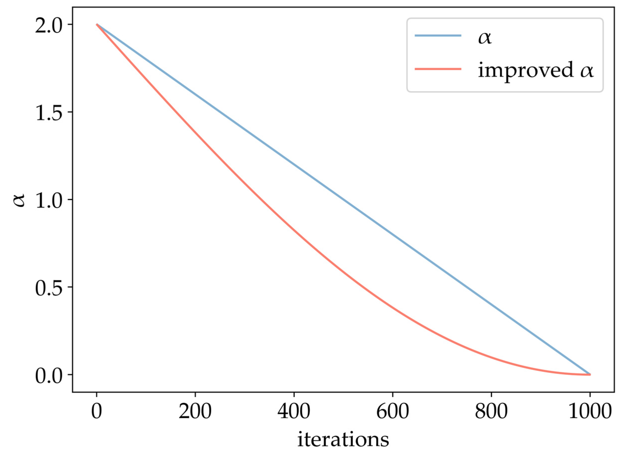
2.5.2. Optimize Control Parameters α

In Equation (17), the value of A in the traditional GWO algorithm is affected by α. The influence of this factor linearly decreased from 2 to 0. For such complex nonlinear problems, as the battery capacity declines, it is impossible to balance the local search and global search energy effectively. Therefore, this paper proposes a method for nonlinear control of the additional variable A.

$$\alpha =2[1-\sin (\frac{\pi }{2}\cdot \frac{i}{I})]$$

(25)

where i is the current iteration number of the α wolf and I denotes the maximum number of iterations. The improved iteration curve for A is shown in Figure 3.

2.5.3. Dynamic Weight

The traditional grey wolf algorithm is a one-way local search, and the position change cannot be changed. In this study, a two-way search was improved, and the selection of a random number control direction was introduced. The search formula is as follows:

$$w=w_{\max }-\frac{i}{I}(w_{\max }-w_{\min })$$

(26)

where w is the weight, w_max is the maximum weight, and w_min is the minimum weight. Generally, when the maximum weight is 0.9 and the minimum weight is 0.4, the algorithm can maintain the best performance [45]. In GWO, the original formula of the inertia weight to change the grey wolf position vector can be introduced on this basis.

$$\left\{\begin{array}{c}\overrightarrow{X_1}=w_{\alpha }\cdot \overrightarrow{X_{\alpha }}-\overrightarrow{A_1}\cdot \overrightarrow{D_{\alpha }}\\ \overrightarrow{X_2}=w_{\beta }\cdot \overrightarrow{X_{\beta }}-\overrightarrow{A_2}\cdot \overrightarrow{D_{\beta }}\\ \overrightarrow{X_3}=w_{\delta }\cdot \overrightarrow{X_{\delta }}-\overrightarrow{A_3}\cdot \overrightarrow{D_{\delta }}\end{array}\right.$$

(27)

$$\left\{\begin{array}{c}{w}_{\alpha }=0.7w_{\alpha }\\ w_{\beta }=0.5w_{\beta }\\ w_{\delta }=0.3w_{\delta }\end{array}\right.$$

(28)

$$X(n+1)=\frac{W_{\alpha }\cdot X_1+W_{\beta }\cdot X_2+W_{\omega }\cdot X_3}{W_{\alpha }+W_{\beta }+W_{\omega }}$$

(29)

where W_α, W_β, and W_δ represent the weights of the wolf population class.

3. Experiment

3.1. Data Sets

To verify the effectiveness and generalization of the method in this study, the datasets including NASA and CALCE were used [46,47]. For the CALCE battery dataset, CS2_35, CS2_36, CS2_37, CS2_38 were selected. The charging and discharging experimental data of the four batteries are used as the input data for the model. All batteries experienced the same charging and discharging modes. At room temperature of 25 °C, the samples were charged at a constant current of 0.5 C. When the voltage reached 4.2 V, they were charged at a constant voltage. When the charging current dropped to 0.05 A, they stopped. The discharge process used 1C current for constant current discharge and stopped when the voltage dropped to 2.7 V.

NASA battery data were selected from B0005, B0006, B0007, and B0018. Under the condition of 24 °C at room temperature, these were charged at a constant current of 1.5 A until the battery voltage reached 4.2 V, and then they were charged at a constant voltage (CV) mode until the charging current dropped to 20 mA. The discharge process was conducted at a constant current (CC) mode of 2 A until the voltage of batteries 5, 6, 7, and 18 dropped to 2.7 V, 2.5 V, 2.2 V, and 2.5 V.

Considering 70% of capacity as the end of life (EOL), NASA’s battery capacity was reduced from 2 Ah to 1.4 Ah. The discharge process was conducted at a constant current (CC) mode of 2 A until the voltage of batteries 5, 6, 7, and 18 dropped to 2.7 V, 2.5 V, 2.2 V, and 2.5 V. The experimental capacity of CACEL was reduced from 1.1 Ah to 0.77 Ah as EOL.

The experimental hardware is configured with Intel Core i5-11320H processor, 16 G RAM, NVIDIA 2070, Windows 11, Python 10.10, and TensorFlow 2.10. First, 50% of the data was used as the training set and test set. After that, 30% of the data was used as the training set, and 70% data was used as the test set to inspect the performance of the model.

3.2. Evaluation Criteria

To evaluate the performance of the prediction model, this paper introduces four evaluation indicators to evaluate the prediction results of the model, which are mean absolute error (MAE), absolute correlation coefficient (R²), and root mean square error (RMSE). MAE can effectively measure the prediction error of the model, and R² reflects the fitting effect of the model. The closer the result, the better the effect [48]. RMSE can measure the prediction accuracy of the model, and its calculation formula is as follows:

$$\mathrm{MAE}=\frac{1}{n}{\displaystyle \sum _{i=1}^n\left|y-\widehat{y}\right|}$$

(30)

$$\mathrm{MSE}=\frac{1}{n}{\displaystyle \sum _{i=1}^n{(y-\widehat{y})}^2}$$

(31)

$$\mathrm{RMSE}=\sqrt{\frac{1}{n}{\displaystyle \sum _{i=1}^n{(y-\widehat{y})}^2}}$$

(32)

$$R^2=1-\frac{{\displaystyle \sum _{i=1}^n{(y-\widehat{y})}^2}}{{\displaystyle \sum _{i=1}^n{(\overline{y}-\widehat{y})}^2}}$$

(33)

where n is the total number of cycles and y and $\hat{y}$ are the actual and predicted values of the battery capacity during the cycle.

In addition, the error calculation index of battery RUL is introduced, and e₁ and e₂ are used to measure the life prediction accuracy. The equation is as follows:

$$e_1=\left|P_{rul}-R_{rul}\right|$$

(34)

$$e_2=\frac{\left|P_{rul}-R_{rul}\right|}{R_{rul}}$$

(35)

In the formula, e₁ and e₂ represent the error and relative error between the actual value and the predicted value of battery RUL, respectively. R_rul represents the actual RUL value, and P_rul represents the predicted RUL value.

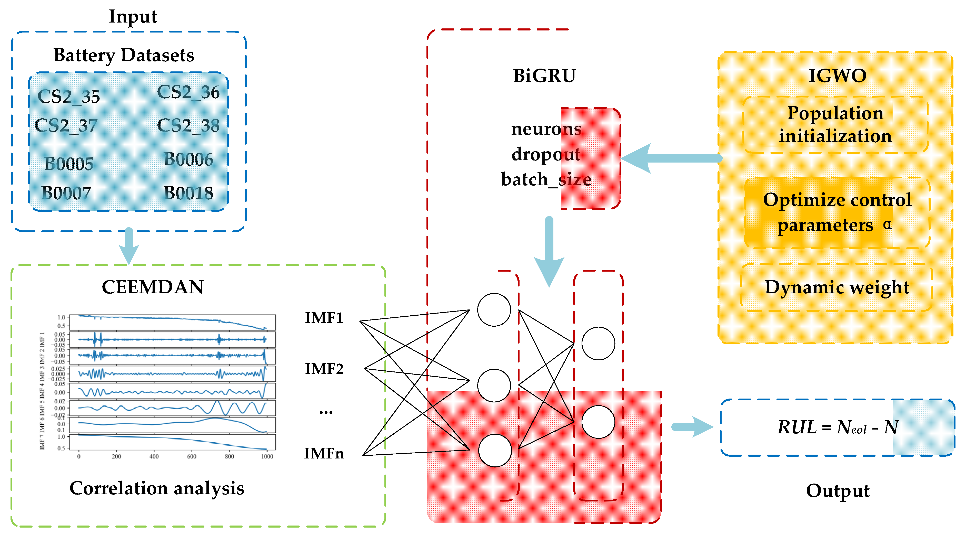
3.3. Structure of the RUL Prediction Model

Combining the advantages and disadvantages of CEEMDAN and BiGRU, the improved Grey Wolf algorithm is used to optimize the parameters of the BiGRU network, and an RUL prediction method based on the CEEMDAN–IGWO–BiGRU model is proposed. The model can reduce the probability of local optimization and over-fitting, and the model design has good robustness. The framework diagram of the RUL estimation is presented in Figure 4. The specific implementation steps are as follows:

Step 1: Collect the battery capacity data and use CEEMDAN to decompose the capacity data into multiple components according to Equations (2)–(7). Divide the training set and test set, and then normalize the data.

Step 2: Determine the number of inputs, output, and hidden layers of the BiGRU, and set parameters such as the number of IGWO populations and the number of iterations.

Step 3: The number of neurons in the input layer of the BiGRU model, number of training samples, and forgetting rate are taken as the individual searchers in the IGWO, and the root mean square error between the expected output of the training samples of the BiGRU model and the actual output is taken as the fitness value. Combined with the improved grey wolf optimization algorithm, the position is continuously updated, and the fitness value is calculated until the conditions are met.

Step 4: Input the obtained optimal weight threshold into the BiGRU model and obtain the IMF prediction results for capacity after training.

4. Results and Discussion

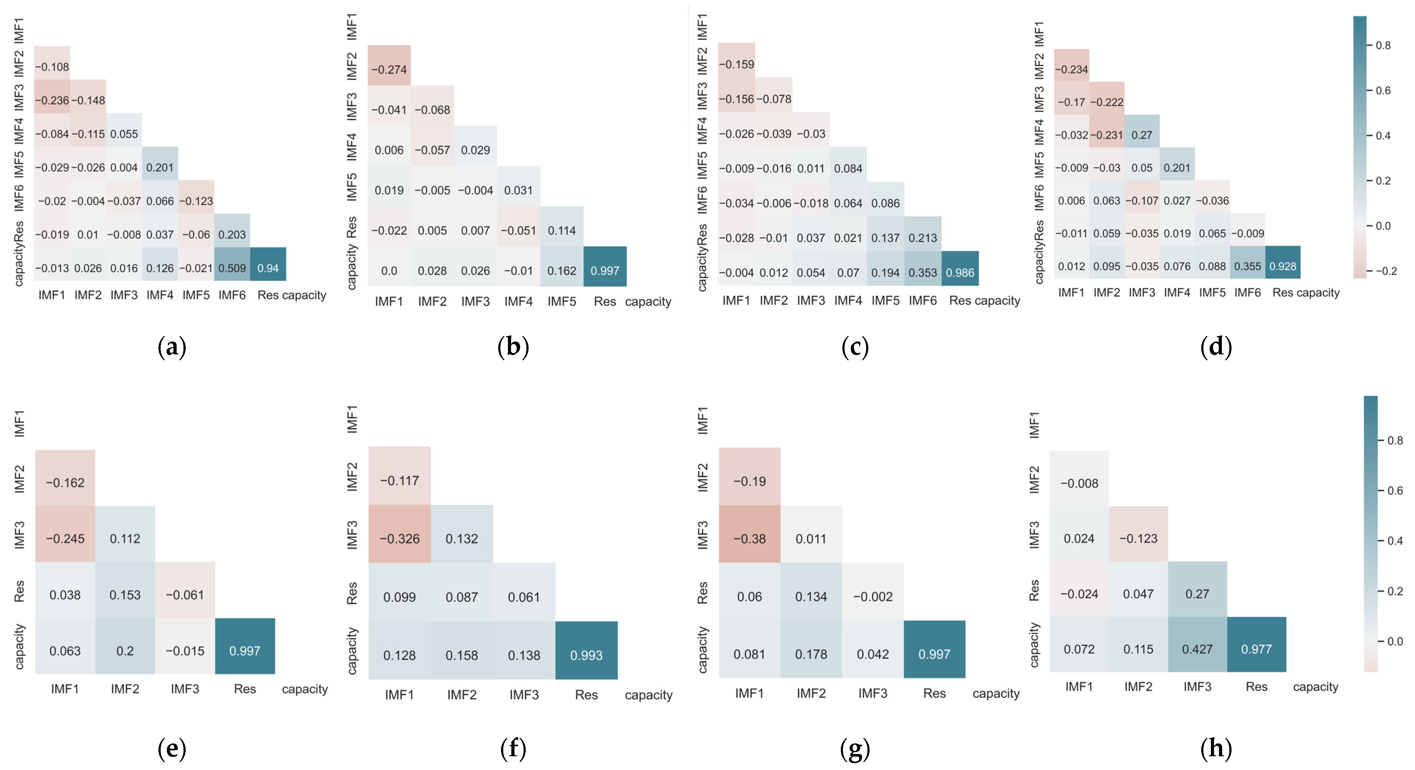
4.1. Results of CEEMDAN

From Figure 5, CEEMDAN can be used to analyze the current change trend and process. Except for CS2_36, other data are decomposed into six intrinsic mode function (IMF) components and one residual signal (Res) component using the CEEMDAN method. CS2_36 can be decomposed into five IMF components, as shown in Figure 5b, and arranged from high to low frequency compared to the degraded sequence of the decomposed modal components and the original capacity. Some modal classifications with low correlation can be discarded as noise.

The correlation between the decomposed variables and battery capacity was analyzed. As shown in Figure 6, the correlation between the original battery capacity and Res is higher than 90%, and Res can effectively reflect the long-term trend of the capacity decline. In addition, the correlation of IMF1, IMF2, and IMF3 in the CALCE dataset was less than 1%, which can be used for noise removal, and the rest of the IMF and Res were used as prediction objects together. In the NASA dataset, IMF components with a correlation greater than 12% are selected as prediction objects.

Decomposing each IMF component, it is difficult to accurately predict the trend of IMF components with low correlation. The signal fluctuation range was within 0.05, and there was no periodicity. After removing the components with less correlation according to the Pearson correlation coefficient, the short-term regeneration trend of the capacity is eliminated, but the overall prediction accuracy of the model can be significantly improved.

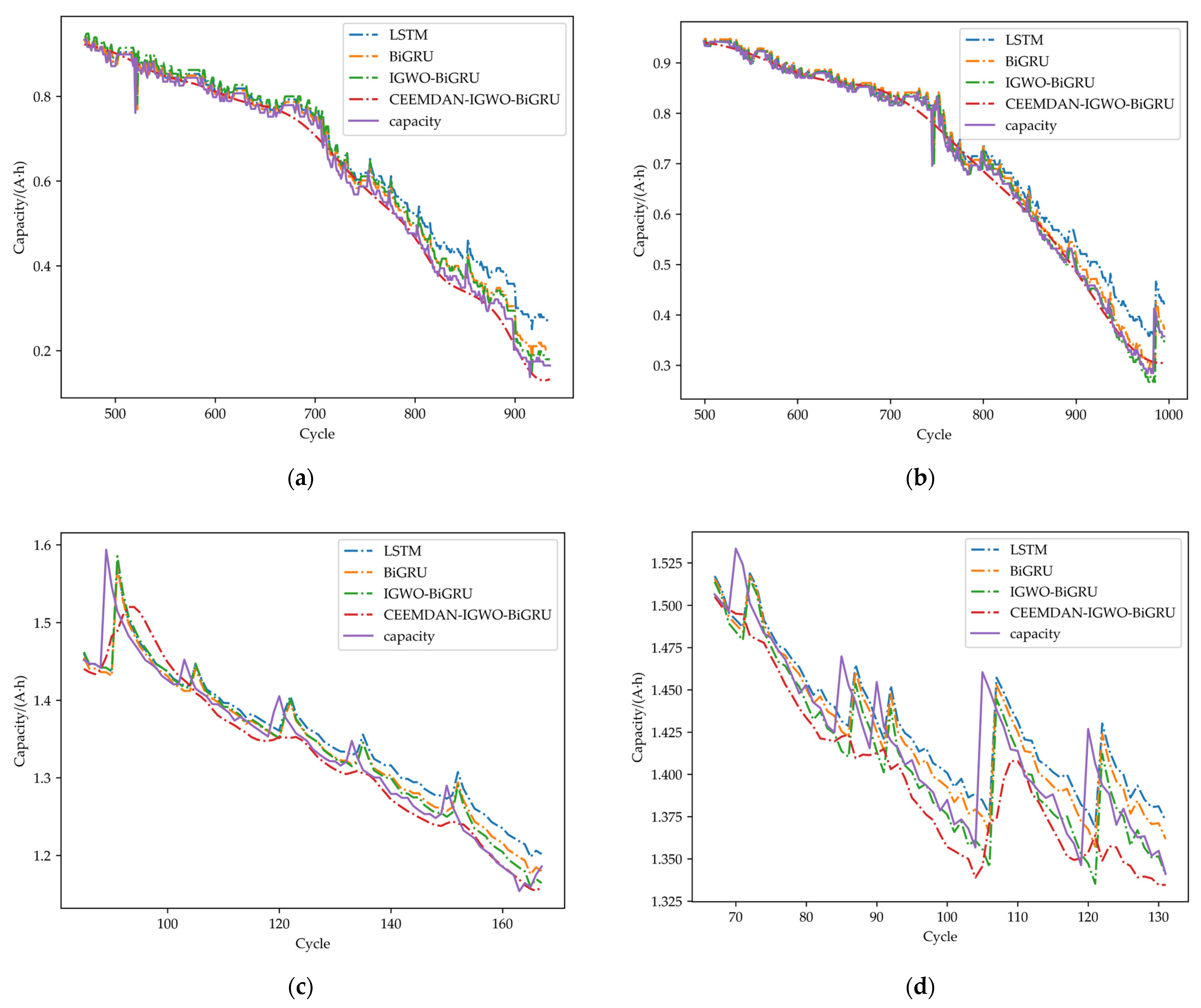
4.2. Results of IGWO–BiGRU

In this study, the IGWO algorithm was used to optimize the parameters of the BiLSTM network model. The BiLSTM in this model selects a sigmoid function as the activation function, including two bidirectional hidden layers. The default number of neurons is 128, the dropout rate is 0.15, the batch size is 128, and the number of iterations is 500. The optimizer is Adam. In the IGWO algorithm, the number of the grey wolf population is defined as 30, and the number of iterations is 5.

During training, 50% was used as the training set. The final prediction results are shown in Figure 7. Under the default parameters, the LSTM model predicts the short-term capacity data accurately. However, with an increase in the number of cycles, the prediction curve gradually deviates. Taking Figure 7b (CS2_38) as an example, the capacity decline trend of 38 batteries increased after 800 cycles. Although the fitting degree of the BiGRU is better than that of LSTM because the default parameters are consistent, there are also deviations for long-term capacity prediction. After using IGWO to optimize the initial parameters, the declining trend of capacity prediction can be consistent with the original value, and the CEEMDAN decomposed and combined curve can better fit the original capacity.

Take Figure 7c,d for example. Owing to the small number of cycles of the NASA dataset, the prediction results of LSTM and the BiGRU deviate laterally from the original capacity, indicating that the prediction method has a certain lag. After using CEEMDAN decomposition to eliminate noise, the reconstructed forecast data were consistent with the actual capacity trend. The combined algorithm can effectively fit the declining trend of the original capacity and avoid premature convergence of the network.

NASA has fewer datasets, and it was necessary to set the EOL to 80% of the capacity. The volume of CALCE data volume was sufficient and the EOL was set as 70% of the capacity for comparison between the models.

Table 1. Lithium battery life prediction error under 50% training set.

Battery	Model	MAE (%)	MSE (%)	RMSE (%)	R2 (%)	e1 (%)	e2 (%)
CS2_35	LSTM	5.63	0.60	7.73	88.92	11	1.74
	BiGRU	4.50	0.39	6.31	92.61	11	1.74
	IGWO–BiGRU	2.73	0.12	3.47	97.77	9	1.43
	CEEMDAN–IGWO–BiGRU	1.35	0.04	2.58	98.96	4	0.63
CS2_36	LSTM	3.91	0.26	5.12	95.20	2	0.38
	BiGRU	3.22	0.19	4.38	96.48	2	0.38
	IGWO–BiGRU	2.46	0.08	2.87	98.49	2	0.38
	CEEMDAN–IGWO–BiGRU	1.57	0.04	2.03	99.23	2	0.38
CS2_37	LSTM	4.19	0.33	5.72	93.12	18	2.57
	BiGRU	3.72	0.28	5.33	94.03	18	2.57
	IGWO–BiGRU	2.51	0.12	3.46	97.47	12	1.71
	CEEMDAN–IGWO–BiGRU	1.36	0.04	1.92	99.06	12	1.71
CS2_38	LSTM	3.00	0.17	4.10	96.96	2	0.27
	BiGRU	2.96	0.16	4.06	97.02	2	0.27
	IGWO–BiGRU	1.73	0.05	2.27	99.06	2	0.27
	CEEMDAN–IGWO–BiGRU	1.36	0.04	1.91	99.06	2	0.27
B0005	LSTM	4.24	0.24	4.91	87.64	78	12.36
	BiGRU	4.25	0.24	4.88	87.78	72	11.41
	IGWO–BiGRU	2.65	0.14	3.79	92.60	26	4.12
	CEEMDAN–IGWO–BiGRU	2.53	0.12	3.46	93.86	11	1.74
B0006	LSTM	4.05	0.20	4.9	85.71	25	41.67
	BiGRU	3.07	0.16	4.04	87.01	25	41.67
	IGWO–BiGRU	2.12	0.11	3.35	91.09	25	41.67
	CEEMDAN–IGWO–BiGRU	1.99	0.10	3.19	91.87	25	41.67
B0007	LSTM	4.05	0.24	4.95	85.71	4	3.25
	BiGRU	3.73	0.22	4.66	87.29	5	4
	IGWO–BiGRU	2.28	0.15	3.89	91.14	3	2.44
	CEEMDAN–IGWO–BiGRU	2.47	0.14	3.68	92.08	7	5.69
B0018	LSTM	4.93	0.30	5.49	64.55	1	1.35
	BiGRU	4.42	0.27	5.18	68.48	1	1.35
	IGWO–BiGRU	2.84	0.28	5.29	67.09	2	2.7
	CEEMDAN–IGWO–BiGRU	3.62	0.23	4.86	72.29	3	4.05

lists the evaluation indicators of the prediction results for the eight lithium-ion batteries under different algorithms. The smaller the RMSE and MAPE, the higher the prediction accuracy of the prediction model. Table 1 shows that the performance indicators predicted by the combined prediction model CEEMDAN–IGWO–BIGRU are superior to other methods, with high accuracy. In the CALCE dataset, the maximum RMSE was less than 2.6% and the maximum MAE was controlled within 1.6% in the NASA dataset. Owing to the lack of data, the model training was insufficient. Taking B0018 as an example, R² was lower than 73% in all the models. It can be observed from the observation of the original data that the sampling time of this battery was relatively discrete, and the number of cycles is 132, which was nearly a quarter less than the sampling data of other batteries, resulting in poor prediction accuracy of the model. In the prediction results of all batteries, the error e₂ of the combined model was controlled under 6%. It is proved that CEEMDAN decomposition and the IGWO algorithm can effectively improve the universality of the model in different application scenarios.

To predict the capacity decline trend in early life, the remaining service life of the lithium-ion battery was measured, and the prediction model was trained using a 30% dataset. The prediction results for the four models are shown in Figure 8.

Because the model training was insufficient, the CALCE dataset had a large deviation in the long-term capacity prediction trend. As shown in Figure 8a, when the number of forecast cycles in the figure was 700, the forecast models deviated from the original capacity curve. However, the CEEMDAN–IGWO–BiGRU model maintained the same declining trend as the original capacity. As shown in Figure 8c, the model proposed in this study is still within the trend of declining range of capacity with 30% training data. It can be seen that the prediction model can still fit the degradation trend of the battery well with less training data, and its stability is better than other algorithms.

Table 2. Lithium battery life prediction error under 30% training set.

Battery	Model	MAE (%)	MSE (%)	RMSE (%)	R2 (%)	e1 (%)	e2 (%)
CS2_35	LSTM	9.68	1.66	12.87	71.15	78	12.36
	BiGRU	9.68	1.66	12.89	71.06	72	11.41
	IGWO–BiGRU	6.02	0.60	7.74	89.55	26	4.12
	CEEMDAN–IGWO–BiGRU	2.45	0.12	3.44	97.94	11	1.74
CS2_36	LSTM	17.18	4.56	21.36	29.28	2	0.27
	BiGRU	15.58	4.11	20.27	36.29	2	0.27
	IGWO–BiGRU	9.44	1.48	12.15	77.11	2	0.27
	CEEMDAN–IGWO–BiGRU	3.74	0.22	4.73	96.54	2	0.27
CS2_37	LSTM	9.19	1.42	11.91	71.60	80	11.41
	BiGRU	8.12	1.23	11.09	75.36	80	11.41
	IGWO–BiGRU	5.05	0.44	6.61	91.25	59	8.42
	CEEMDAN–IGWO–BiGRU	3.98	0.20	4.53	95.90	50	7.13
CS2_38	LSTM	5.65	0.61	7.78	89.43	2	0.27
	BiGRU	5.54	0.58	7.61	89.89	2	0.27
	IGWO–BiGRU	3.74	0.27	5.18	95.33	2	0.27
	CEEMDAN–IGWO–BiGRU	2.56	0.10	3.13	98.29	2	0.27
B0005	LSTM	26.08	7.85	28.02	-47.88	2	2
	BiGRU	25.94	7.73	27.81	-45.60	1	1
	IGWO–BiGRU	17.89	3.71	19.25	30.21	0	0
	CEEMDAN–IGWO–BiGRU	3.45	0.41	6.16	89.24	0	0
B0006	LSTM	8.78	0.90	9.50	63.92	5	6.37
	BiGRU	8.39	0.84	9.18	66.34	5	6.37
	IGWO–BiGRU	5.53	0.38	6.18	84.73	2	3.1
	CEEMDAN–IGWO–BiGRU	2.88	0.12	3.46	95.20	2	3.1
B0007	LSTM	21.00	4.99	22.33	-13.33	7	5.69
	BiGRU	21.38	5.18	22.76	-17.70	5	4.07
	IGWO–BiGRU	13.00	1.92	13.86	56.33	3	2.44
	CEEMDAN–IGWO–BiGRU	5.27	0.33	5.73	92.54	3	2.44
B0018	LSTM	6.72	0.62	7.84	84.44	4	5.41
	BiGRU	6.39	0.58	7.62	85.31	4	5.41
	IGWO–BiGRU	5.10	0.43	6.54	89.20	2	2.7
	CEEMDAN–IGWO–BiGRU	3.57	0.40	6.30	89.97	2	2.7

summarizes the predicted performance indicators of all lithium-ion batteries in the 30% training set. It can be observed from Table 2 that the prediction effect of LSTM and the BiGRU is poor owing to the influence of the training data. The CALCE dataset exhibits capacity regeneration when reaching EOL, and the amplitude range is large. In CS2_37, the RUL error was significantly greater than those of the other three batteries, although the RMSE of the hybrid method was 4.53%. In addition, CEEMDAN–IGWO–BiGRU maintained a high accuracy rate, with a maximum MAE of less than 4%.

The MAE of B0005 and B0007 in the NASA battery set was up to 20%. The MAE of CEEMDAN–IGWO–BiGRU could still be maintained below 3.5. Owing to the small number of datasets, the relative error of the RUL could be controlled within 3.5%, showing strong robustness. The IGWO significantly improves the stability of the network prediction. The combined prediction algorithm fully trained the data, improved the prediction accuracy, and reduced the strong dependence on the data. In addition, in CS_ 38 and B0018, CEEMDAN had limited improvement in model accuracy. The main reason for this is that some IMF components with weak correlations were removed. Although the predicted capacity curve maintains the global declining trend after noise elimination, it cannot predict the change in capacity regeneration at high frequencies in the short term.

5. Conclusions

In this study, a CEEMDAN–IGWO–BiLSTM model was proposed to predict the capacity and RUL of lithium batteries. The following conclusions were drawn from previous research. The CEEMDAN algorithm is used to effectively solve the mode aliasing problem after the initial current data decomposition and to reduce the error caused by the current data instability in the prediction process. The CEEMDAN–BiGRU model, which uses the IMF component as the model input and capacity values as the output, is suitable for RUL prediction under various working conditions. The GWO algorithm was improved by the nonlinear control of variable A. Additionally, tent mapping improved the global search ability and convergence speed of the GWO algorithm. The improved GWO algorithm was used to optimize the weight and threshold of the BiGRU prediction model to obtain the best parameters. Through simulation and comparison with LSTM and BiGRU, the improved GWO algorithm can further explore the relationship between the IMF component of capacity and RUL. Both the MAE and RMSE were less than 6.3% when only 30% of the dataset was used. Moreover, the accuracy and stability of the RUL prediction of the battery were improved using the hybrid model. The relative error of the RUL was less than 7.13%.

References

1. Larcher, D.; Tarascon, J.M. Towards greener and more sustainable batteries for electrical energy storage. Nat. Chem. 2015, 7, 19–29. [Google Scholar] [CrossRef] [PubMed]
2. Mohamed, S.M.; Sanad, M.M.S.; Mattar, T.; El-Shahat, M.F.; Rossignol, C.; Dessemond, L.; Zaidat, K.; Obbade, S. The Structural, Thermal and Electrochemical Properties of MnFe1−x−yCuxNiyCoO4 Spinel Protective Layers in Interconnects of Solid Oxide Fuel Cells (SOFCs). J. Alloy. Compd. 2022, 923, 166351. [Google Scholar] [CrossRef]
3. Harbaoui, D.; Sanad, M.M.S.; Rossignol, C.; Hlil, E.K.; Amdouni, N.; Zaidat, K.; Obbade, S. Effect of Divalent Transition Metal Ions on Physical, Morphological, Electrical and Electrochemical Properties of Alluaudite Phases Na2M2 + 2Fe3+(PO4)3 (M = Mn, Co and Ni): Cathode Materials for Sodium-Ions Batteries. J. Alloys Compd. 2022, 901, 163641. [Google Scholar] [CrossRef]
4. Hannan, M.A.; Lipu, M.H.; Hussain, A.; Mohamed, A. A review of lithium-ion battery state of charge estimation and management system in electric vehicle applications: Challenges and recommendations. Renew. Sustain. Energy Rev. 2017, 78, 834–854. [Google Scholar] [CrossRef]
5. Jaguemont, J.; Boulon, L.; Dubé, Y. A comprehensive review of lithium-ion batteries used in hybrid and electric vehicles at cold temperatures. Appl. Energy 2016, 164, 99–114. [Google Scholar] [CrossRef]
6. Han, X.; Lu, L.; Zheng, Y.; Feng, X.; Li, Z.; Li, J.; Ouyang, M. A review on the key issues of the lithium ion battery degradation among the whole life cycle. ETransportation 2019, 1, 100005. [Google Scholar] [CrossRef]
7. Duan, J.; Tang, X.; Dai, H.; Yang, Y.; Wu, W.; Wei, X.; Huang, Y. Building safe lithium-ion batteries for electric vehicles: A review. Electrochem. Energy Rev. 2020, 3, 1–42. [Google Scholar] [CrossRef] [Green Version]
8. Chen, M.; Ma, X.; Chen, B.; Arsenault, R.; Karlson, P.; Simon, N.; Wang, Y. Recycling end-of-life electric vehicle lithium-ion batteries. Joule 2019, 3, 2622–2646. [Google Scholar] [CrossRef]
9. Makuza, B.; Tian, Q.; Guo, X.; Chattopadhyay, K.; Yu, D. Pyrometallurgical options for recycling spent lithium-ion batteries: A comprehensive review. J. Power Sources 2021, 491, 229622. [Google Scholar] [CrossRef]
10. Guha, A.; Patra, A. State of health estimation of lithium-ion batteries using capacity fade and internal resistance growth models. IEEE Trans. Transp. Electrif. 2017, 4, 135–146. [Google Scholar] [CrossRef]
11. Severson, K.A.; Attia, P.M.; Jin, N.; Perkins, N.; Jiang, B.; Yang, Z.; Braatz, R.D. Data-driven prediction of battery cycle life before capacity degradation. Nat. Energy 2019, 4, 383–391. [Google Scholar] [CrossRef] [Green Version]
12. Xiong, R.; Cao, J.; Yu, Q.; He, H.; Sun, F. Critical review on the battery state of charge estimation methods for electric vehicles. IEEE Access 2017, 6, 1832–1843. [Google Scholar] [CrossRef]
13. Sanad, M.M.; Meselhy, N.K.; El-Boraey, H.A.; Toghan, A. Controllable engineering of new ZnAl2O4-decorated LiNi0· 8Mn0· 1Co0· 1O2 cathode materials for high performance lithium-ion batteries. J. Mater. Res. Technol. 2023, 23, 1528–1542. [Google Scholar] [CrossRef]
14. Babaeiyazdi, I.; Rezaei-Zare, A.; Shokrzadeh, S. State of charge prediction of EV Li-ion batteries using EIS: A machine learning approach. Energy 2021, 223, 120116. [Google Scholar] [CrossRef]
15. Ren, L.; Dong, J.; Wang, X.; Meng, Z.; Zhao, L.; Deen, M.J. A data-driven auto-CNN-LSTM prediction model for lithium-ion battery remaining useful life. IEEE Trans. Ind. Inform. 2020, 17, 3478–3487. [Google Scholar] [CrossRef]
16. Zhao, S.; Zhang, C.; Wang, Y. Lithium-ion battery capacity and remaining useful life prediction using board learning system and long short-term memory neural network. J. Energy Storage 2022, 52, 104901. [Google Scholar] [CrossRef]
17. Yao, F.; He, W.; Wu, Y.; Ding, F.; Meng, D. Remaining useful life prediction of lithium-ion batteries using a hybrid model. Energy 2022, 248, 123622. [Google Scholar] [CrossRef]
18. Liu, K.; Shang, Y.; Ouyang, Q.; Widanage, W.D. A data-driven approach with uncertainty quantification for predicting future capacities and remaining useful life of lithium-ion battery. IEEE Trans. Ind. Electron. 2020, 68, 3170–3180. [Google Scholar] [CrossRef]
19. Zhou, D.; Li, Z.; Zhu, J.; Zhang, H.; Hou, L. State of health monitoring and remaining useful life prediction of lithium-ion batteries based on temporal convolutional network. IEEE Access 2020, 8, 53307–53320. [Google Scholar] [CrossRef]
20. Cheng, G.; Wang, X.; He, Y. Remaining useful life and state of health prediction for lithium batteries based on empirical mode decomposition and a long and short memory neural network. Energy 2021, 232, 121022. [Google Scholar] [CrossRef]
21. Chen, L.; Zhang, Y.; Zheng, Y.; Li, X.; Zheng, X. Remaining useful life prediction of lithium-ion battery with optimal input sequence selection and error compensation. Neurocomputing 2020, 414, 245–254. [Google Scholar] [CrossRef]
22. Cao, J.; Li, Z.; Li, J. Financial time series forecasting model based on CEEMDAN and LSTM. Phys. A: Stat. Mech. Its Appl. 2019, 519, 127–139. [Google Scholar] [CrossRef]
23. Yun, Z.; Qin, W.; Shi, W.; Ping, P. State-of-health prediction for lithium-ion batteries based on a novel hybrid approach. Energies 2020, 13, 4858. [Google Scholar] [CrossRef]
24. Meng, H.; Geng, M.; Xing, J.; Zio, E. A hybrid method for prognostics of lithium-ion batteries capacity considering regeneration phenomena. Energy 2022, 261, 125278. [Google Scholar] [CrossRef]
25. Qu, J.; Liu, F.; Ma, Y.; Fan, J. A neural-network-based method for RUL prediction and SOH monitoring of lithium-ion battery. IEEE Access 2019, 7, 87178–87191. [Google Scholar] [CrossRef]
26. Chen, G.; Tang, B.; Zeng, X.; Zhou, P.; Kang, P.; Long, H. Short-term wind speed forecasting based on long short-term memory and improved BP neural network. Int. J. Electr. Power Energy Syst. 2022, 134, 107365. [Google Scholar] [CrossRef]
27. Karijadi, I.; Chou, S.Y. A hybrid RF-LSTM based on CEEMDAN for improving the accuracy of building energy consumption prediction. Energy Build. 2022, 259, 111908. [Google Scholar] [CrossRef]
28. Ding, G.; Wang, W.; Zhu, T. Remaining Useful Life Prediction for Lithium-Ion Batteries Based on CS-VMD and GRU. IEEE Access 2022, 10, 89402–89413. [Google Scholar] [CrossRef]
29. Gao, B.; Huang, X.; Shi, J.; Tai, Y.; Zhang, J. Hourly forecasting of solar irradiance based on CEEMDAN and multi-strategy CNN-LSTM neural networks. Renew. Energy 2020, 162, 1665–1683. [Google Scholar] [CrossRef]
30. Mirjalili, S.; Mirjalili, S.M.; Lewis, A. Grey wolf optimizer. Adv. Eng. Softw. 2014, 69, 46–61. [Google Scholar] [CrossRef] [Green Version]
31. Dokeroglu, T.; Sevinc, E.; Kucukyilmaz, T.; Cosar, A. A survey on new generation metaheuristic algorithms. Comput. Ind. Eng. 2019, 137, 106040. [Google Scholar] [CrossRef]
32. Abualigah, L.; Diabat, A.; Mirjalili, S.; Abd Elaziz, M.; Gandomi, A.H. The arithmetic optimization algorithm. Comput. Methods Appl. Mech. Eng. 2021, 376, 113609. [Google Scholar] [CrossRef]
33. Altan, A.; Karasu, S.; Zio, E. A new hybrid model for wind speed forecasting combining long short-term memory neural network, decomposition methods and grey wolf optimizer. Appl. Soft Comput. 2021, 100, 106996. [Google Scholar] [CrossRef]
34. Nadimi-Shahraki, M.H.; Taghian, S.; Mirjalili, S. An improved grey wolf optimizer for solving engineering problems. Expert Syst. Appl. 2021, 166, 113917. [Google Scholar] [CrossRef]
35. Long, W.; Cai, S.; Jiao, J.; Xu, M.; Wu, T. A new hybrid algorithm based on grey wolf optimizer and cuckoo search for parameter extraction of solar photovoltaic models. Energy Convers. Manag. 2020, 203, 112243. [Google Scholar] [CrossRef]
36. Zhao, X.; Zhang, X.; Cai, Z.; Tian, X.; Wang, X.; Huang, Y.; Hu, L. Chaos enhanced grey wolf optimization wrapped ELM for diagnosis of paraquat-poisoned patients. Comput. Biol. Chem. 2019, 78, 481–490. [Google Scholar] [CrossRef]
37. Hu, X.; Xu, L.; Lin, X.; Pecht, M. Battery lifetime prognostics. Joule 2020, 4, 310–346. [Google Scholar] [CrossRef]
38. Meng, X.; Cai, C.; Wang, Y.; Wang, Q.; Tan, L. Remaining useful life prediction of lithium-ion batteries using CEEMDAN and WOA-SVR model. Front. Energy Res. 2022, 10, 1460. [Google Scholar] [CrossRef]
39. Qu, W.; Chen, G.; Zhang, T. An Adaptive Noise Reduction Approach for Remaining Useful Life Prediction of Lithium-Ion Batteries. Energies 2022, 15, 7422. [Google Scholar] [CrossRef]
40. Jiao, M.; Wang, D.; Qiu, J. A GRU-RNN based momentum optimized algorithm for SOC estimation. J. Power Sources 2020, 459, 228051. [Google Scholar] [CrossRef]
41. Bao, Z.; Jiang, J.; Zhu, C.; Gao, M. A new hybrid neural network method for state-of-health estimation of lithium-ion battery. Energies 2022, 15, 4399. [Google Scholar] [CrossRef]
42. Mellit, A.; Pavan, A.M.; Lughi, V. Deep learning neural networks for short-term photovoltaic power forecasting. Renew. Energy 2021, 172, 276–288. [Google Scholar] [CrossRef]
43. Heidari, A.A.; Mirjalili, S.; Faris, H.; Aljarah, I.; Mafarja, M.; Chen, H. Harris hawks optimization: Algorithm and applications. Future Gener. Comput. Syst. 2019, 97, 849–872. [Google Scholar] [CrossRef]
44. Mirjalili, S.; Saremi, S.; Mirjalili, S.M.; Coelho, L.D.S. Multi-objective grey wolf optimizer: A novel algorithm for multi-criterion optimization. Expert Syst. Appl. 2016, 47, 106–119. [Google Scholar] [CrossRef]
45. Yin, C.; Mao, S. Fractional multivariate grey Bernoulli model combined with improved grey wolf algorithm: Application in short-term power load forecasting. Energy 2023, 269, 126844. [Google Scholar] [CrossRef]
46. Liu, D.; Zhou, J.; Pan, D.; Peng, Y.; Peng, X. Lithium-ion battery remaining useful life estimation with an optimized relevance vector machine algorithm with incremental learning. Measurement 2015, 63, 143–151. [Google Scholar] [CrossRef]
47. Liu, D.; Luo, Y.; Liu, J.; Peng, Y.; Guo, L.; Pecht, M. Lithium-ion battery remaining useful life estimation based on fusion nonlinear degradation AR model and RPF algorithm. Neural Comput. Appl. 2014, 25, 557–572. [Google Scholar] [CrossRef]
48. Wang, C.; Lu, N.; Wang, S.; Cheng, Y.; Jiang, B. Dynamic long short-term memory neural-network-based indirect remaining-useful-life prognosis for satellite lithium-ion battery. Appl. Sci. 2018, 8, 2078. [Google Scholar] [CrossRef] [Green Version]
Figure 1. Structure of the BiGRU.
Sustainability 15 06261 g001
Figure 2. Hierarchy of grey wolves.
Sustainability 15 06261 g002
Figure 3. Changes in control parameter α.
Sustainability 15 06261 g003
Figure 4. The framework diagram of the RUL estimation.
Sustainability 15 06261 g004
Figure 5. Decomposition results of CALCE and NASA. (a) CS2_35. (b) CS2_36. (c) CS2_37. (d) CS2_38. (e) B0005. (f) B0006. (g) B0007. (h) B0018.
Sustainability 15 06261 g005aSustainability 15 06261 g005b
Figure 6. The correlation coefficient between the original capacity and the decomposed IMF. (a) CS2_35. (b) CS2_36. (c) CS2_37. (d) CS2_38. (e) B0005. (f) B0006. (g) B0007. (h) B0018.
Sustainability 15 06261 g006
Figure 7. 50% training set lithium-ion battery prediction results. (a) CS2_36. (b) CS2_38. (c) B0005. (d) B0018.
Sustainability 15 06261 g007
Figure 8. 30% training set lithium-ion battery prediction results. (a) CS2_36. (b) CS2_38. (c) B0005. (d) B0008.
Sustainability 15 06261 g008