Article

Design of a Telepresence Robot to Avoid Obstacles in IoT-Enabled Sustainable Healthcare Systems

by
Ali A. Altalbe
1,2,*,
Muhammad Nasir Khan
3,* and
Muhammad Tahir
4
1
Computer Engineering Department, Prince Sattam Bin Abdulaziz University, Al-Kharj 11942, Saudi Arabia
2
Faculty of Computing and Information Technology, King Abdulaziz University, Jeddah 21589, Saudi Arabia
3
Electrical Engineering Department, GC University Lahore, Lahore 54000, Pakistan
4
Software Engineering Department, Sir Syed University of Engineering and Technology, Karachi 75300, Pakistan
*
Authors to whom correspondence should be addressed.
Sustainability 2023, 15(7), 5692; https://doi.org/10.3390/su15075692
Submission received: 4 February 2023 / Revised: 6 March 2023 / Accepted: 12 March 2023 / Published: 24 March 2023
(This article belongs to the Special Issue IoT Quality Assessment and Sustainable Optimization)

Abstract

:
In the Internet of Things (IoT) era, telepresence robots (TRs) are increasingly a part of healthcare, academia, and industry due to their enormous benefits. IoT provides a sensor-based environment in which robots receive more precise information about their surroundings. The researchers work day and night to reduce cost, duration, and complexity in all application areas. It provides tremendous benefits, such as sustainability, welfare improvement, cost-effectiveness, user-friendliness, and adaptability. However, it faces many challenges in making critical decisions during motion, which requires a long training period and intelligent motion planning. These include obstacle avoidance during movement, intelligent control in hazardous situations, and ensuring the right measurements. Following up on these issues requires a sophisticated control design and a secure communication link. This paper proposes a control design to normalize the integration process and offer an auto-MERLIN robot with cognitive and sustainable architecture. A control design is proposed through system identification and modeling of the robot. The robot control design was evaluated, and a prototype was prepared for testing in a hazardous environment. The robot was tested by considering various parameters: driving straight ahead, turning right, self-localizing, and receiving commands from a remote location. The maneuverability, controllability, and stability results show that the proposed design is well-developed and cost-efficient, with a fast response time. The experimental results show that the proposed method significantly minimizes the obstacle collisions. The results confirm the employability and sustainability of the proposed design and demonstrate auto-MERLIN’s capabilities as a sustainable robot ready to be deployed in highly interactive scenarios.

1. Introduction

In the modern era, human–robot interaction is increasing in scope and demand in many application areas, including healthcare systems and military applications. This is due to the advancement and capability of robots to perform complex tasks in dangerous and/or prohibited environments. The evolution of the digital era and smart robotic designs continue to simplify daily routine tasks with fast response times and precision [1,2,3]. Researchers are working very hard to design such robots; nonetheless, they have many limitations in performing various functions. On the other hand, it has become necessary for humans to involve robots in tasks from remote locations or in harmful situations, e.g., COVID-19. Robots are controlled by human beings who execute scheduled tasks from remote locations [4,5,6]. These systems aim to capture the environment appropriately and to maneuver based on acquired knowledge [7,8,9,10,11].
This paper aims to analyze system identification parameters and robot behavior, and to stabilize the nonlinear behavior by designing a control system. This paper presents a design using system modelling and develops an analysis of stability. The challenge may be understood as investigating the feasibility of designing an autonomous robot with the capacity to plan its actions to accomplish specified tasks. For that purpose, we emphasized design aspects, including identification and stability analysis. Furthermore, verification will be made possible almost from implementation up to high-level mission specification, in which models based on state transition systems are used [1].
In the presented research work, a mobile robot based on the chassis of a vehicle model was developed. In particular, a microcontroller-based control was developed to control the robot’s behavior depending on user preferences and environmental influences and controls. The robot chassis was modified as per the designed control actuators and sensors [12,13,14,15]; it included small, necessary mechanical structures. We intend to develop a control program to evaluate the measured values of various sensors, and then to send appropriate control variables to the actuators. In addition, the controller was equipped with a communications interface, allowing it to coordinate with a superior level of control. A teleoperator directly operated the robot. It contained the user program, with which the user was able to parameterize the robot. The computer also had a wireless interface used to operate the robot wirelessly. This basic framework is necessary for the user program which executes the mini-computer.
Subsequently, the robot’s behavior was examined theoretically. From these findings, the most optimal settings were then determined for the robot. Finally, some test scenarios were run with the robot so that its real behavior could be determined, which were predicted to prove roughly similar to the desired behavior. This proposed approach differs from previous approaches [16,17] in many ways. The proposed approach is a controller-based approach, rather than one based on big data. The control method is very flexible and can be implemented for dynamic obstacles. The proposed self-localization procedure is very simple, giving a small error in orientations. There are many benefits of the proposed approach, as follows:
  • The method is more adaptable in terms of implementation;
  • The computational complexity is comparatively low compared to other machine learning methods;
  • By employing this technique, we can achieve virtual doctor–patient interactions in any difficult and hazardous situation.

2. Background

In the recent era, the social lives of human beings have depended on technology. Although technologies have greatly improved the lifestyle of human beings, including in the workplace and social gatherings, more investigation can be undertaken to achieve customer satisfaction and systematic analysis [18,19,20,21,22,23]. TRs and autonomous vehicles (AVs) might be attractive alternatives in the human social ecosystem. In [24], a remote manipulator, considered the pioneer robotic arm, was implemented. Implementing these TRs is useful in a COVID-19 or otherwise hazardous environment that is inaccessible to humans [25,26,27,28]. In [29], researchers developed TRs for offices, healthcare systems, and nursing homes. Another useful application is augmented virtual reality, which is useful to simulate the feeling of a human–robot interactive environment [30,31,32,33]. In [34], immersed virtual reality was developed to provide guidelines for user design. Many challenges remain, including the implementation of adjustable height [22], motion along the slope surface [35], system stability [36], and low-speed control [37,38,39,40,41].
The well-known application areas of mobile robots include ocean exploration, approaching the moon, implementation in nuclear plants [42,43,44,45], and, recently, COVID-19 [46,47,48,49,50]. It is often difficult to repair in such scenarios; therefore, the alternate approach of a mobile robot to accomplishing these tasks from a remote location is quite demanding. In addition, the negotiation with the end consumer is condensed to mission provisions, and then automating mobile robots’ communications with experts minimize it. Total operational autonomy is also required, especially in perception, decision, and control. However, the specificity of the application domain generates particular constraints which may sometimes be antagonistic, according to the relevant scientific discipline [36,37]. The trajectory control in the software architecture of TRs is presented by [22,50,51,52,53,54] in a dynamic traffic environment. Telepresence robots are utilized in many applications, and have shown tremendous results in human–robot interactions [49,50].
A more general architecture of the telepresence robot is presented in [26,37]. A telepresence robot comprises both software and hardware architectures. It contains hardware components, e.g., biosensors, which obtain information from the patient and send it to the consultant at a remote location using the available communication technology [6,10,38]. It also contains components which can produce the control inputs necessary for the robot to move in a stable position using the actuator connected to it. These actuators control the hardware actions, e.g., motion, speed, and position [39,40,41]. The presented work focuses on the identification and stabilization of the TR and the development of micro-controller-based architecture. The core responsibility of the design is to control the driving behavior and to avoid obstacles in the TR’s track The design also contains the module with the best driving path, called the decision-making module. The function of this module is to provide the best path and safe driving with obstacle avoidance control. The term “maneuver” is most likely utilized in the literature to describe path planning. Still, for clarity and consistency, the term “behavior” is employed to label the entire journey of the presented research article. According to the activities generated by the mini-computer in computing, this study also considered other independent attributes such as position, trajectory, orientation, and speed.
Much research has been conducted in the healthcare system using the methods outlined in [55,56,57,58]. The benefits of employing these approaches in the healthcare environment have been evident during the COVID-19 pandemic, when it was required that doctors keep physical distance from their patients to protect themselves. However, to further improve and diagnose the patient, doctors must interact with them; here, the demand for telepresence robots arises. To send robots to the patient ward, care must be taken to avoid collisions of the robots with various obstacles in the hospital environment. Researchers need to propose algorithms for the proper operation of telepresence robots. Each approach has its pros and cons, the proposed approach included, and the idea is to implant a telepresence robot into the hospital environment with fewer obstacles. Utilizing the proposed approach, the doctors help to obtain an initial interaction with the patient and the telepresence robot while maintaining a safe distance. The first try was conducted considering the parameters given in Table 1.
A review of the literature review found that most human–robot interactions were implemented efficiently, except for disconnection or delays [55]. The proposed approach is comparatively easy to implement, more flexible, and efficient. Further, various factors, e.g., design variations and human interaction deficiencies, were discussed in terms of the capability of object avoidance and new peripheral connection to exhibit better human-like behavior remotely.
The research gaps have been clearly mentioned and are now highlighted as:
  • There is a dire demand for a telepresence robot to be designed that could be utilized in the pandemic situation. A safe physical distance between the target and the transmitter is usually required.
  • The design of such a robot, capable of human–robot interaction, is a popular topic to explore, and is receiving much attention in academia, industry, and healthcare systems.
The telepresence robot is an extremely nonlinear system with a gearbox for power transmission, and its precise mathematical model is not simple to derive. Therefore, a system identification approach was implemented to find the approximate model of the system [59]. The root locus method was used to design a speed controller by introducing appropriate poles and zeros [59]. The results validated the identified model of the system. The results were also compared with the A* algorithm [60] to highlight the importance of the proposed work.
A more generalized diagram is shown in Figure 1, equipped with a telepresence robot (auto-MERLIN). The mobile robot aimed to equip auto-MERLIN to leave prescribed paths, navigate, detect obstacles, and avoid them. It required entirely new control electronics to be developed. The robot utilized the powerful direct current (DC) motor TruckPuller3 7.2 V for the drive and the powerful model-equipped servo motor HiTec HS-5745MG for steering [16]. The drive motor was equipped with an optical position encoder from the company M101B MEGATRON Elektronik AG & Co. [17], which the speed and direction can determine.
The TR is designed to maneuver around in dynamic environments (i.e., offices), encountering fixes and moving obstacles. It is worth underscoring the challenges for the telepresence robot while maneuvering in a distant place, controlled by a commanding user. There are various approaches which are worth mentioning. The background section can be further enhanced by adding the following approaches, with each approach’s limitation given in Table 2.
None of the previous studies considered a non-technologically-oriented controller to operate telepresence robots remotely. It is not possible for a telepresence robot to be used as a simple on–off to cover all behaviors displayed by remote telepresence robots. Despite a simple user controller technique, it appears that previous telepresence robot controllers had no control over expressive material, nor what we consider to be the need to rationalize the design to control telepresence robots. Our discussion and the above observation affect the number of new features that can be added to the telepresence robot, and the addition of some more specific controlling techniques is required.

3. System Design and Implementation

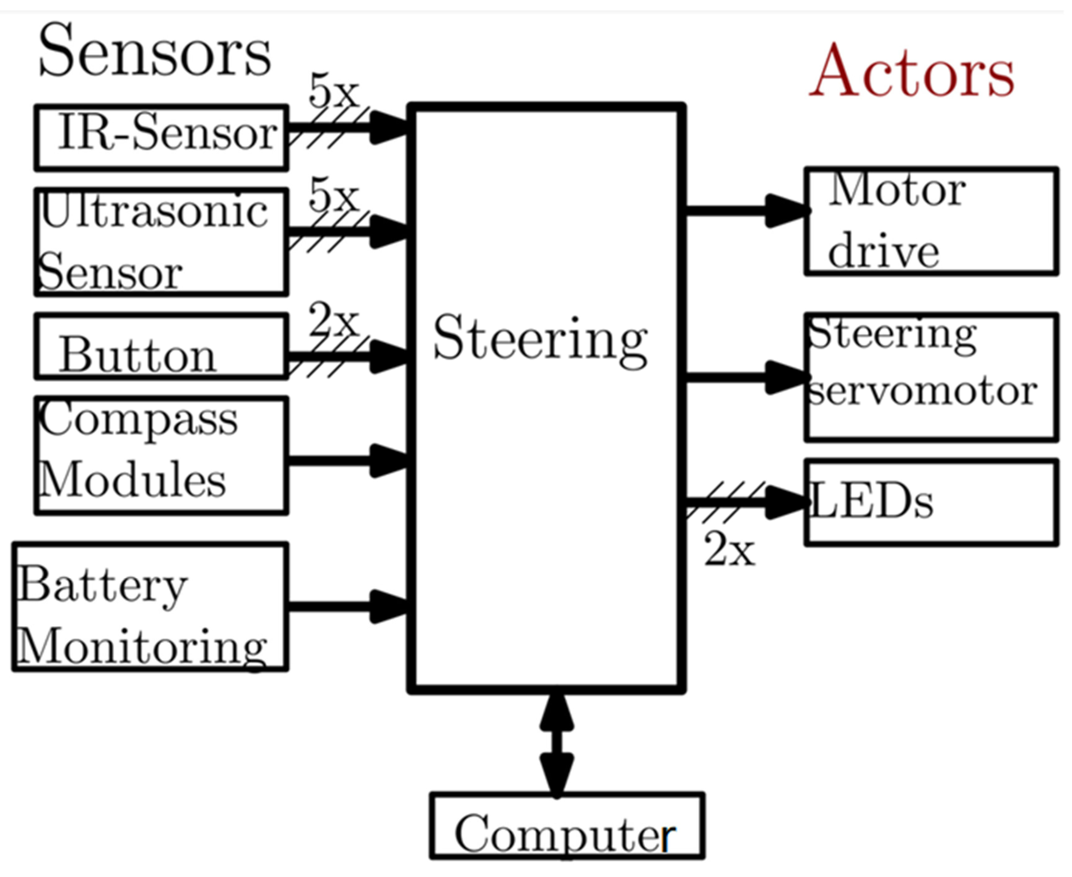
Before starting the hardware design, the mobile robot’s actuators and sensors operations are worth mentioning; they are the main actuators of the first two pre-built engines. First, the direct-current (DC) motor for driving TruckPuller2 of 7.2 V and the other in the longitudinal direction of the servo motor is used (HiTec HS-5745MG [13]) for steering. It is complemented by one red and one green light-emitting diode (LED) to indicate the state of the robot later. Sensors, which detect the robot’s state and environment, require much more input. The list begins with state detection sensors for the robot. The drive motor is already equipped with the position encoder M101B [14], so the exact engine speed and, thus, the approximate distance of the robot can be determined. The steering does not use a separate sensor to measure the steering angle. Herein, it is assumed that the built-in servo motor control for steering is precise. A compass module is used as an additional sensor, and can detect magnetic fields in all three spatial directions. Using the magnetic field measurements on the Earth’s magnetic field, the absolute orientation of the robot can be determined. The absolute position is elicited through the odometry method.
Now, the environmental sensors are to be measured at five discrete angles, each having an infrared sensor and an ultrasonic distance to an object. Using this distance measurement will later allow us to bypass obstacles. Two more buttons are provided, but in the context of this presented work, they have no meaning. Furthermore, this logic supplies the voltage of the battery and powers the drive, which is monitored by the controller. All of these actuators and sensors must be combined into one control device. Therefore, a separate control board was developed in the context of this work. This control board can communicate via an EIA-232 interface with a mini-computer. Figure 2 shows the structure of the sensors and actuators.
To keep undesirable parasitic inductances and capacitances as low as possible, the freewheeling diode of the switching regulator should be positioned close to the switching regulator integrated circuit (IC). Since the switching regulator’s large currents quickly switched to 260 kHz, the structure should be as compact as possible and immediately adjacent to the battery connector. In addition, a large area of the surface should be measured below the control to avoid directly derived disturbance. The switching regulator supplies 8 V and 40 V voltage on the input side. The minimum required output current of the controller for proper operation is 20 mA. The On/Off pin of the regulator ICs should not be connected to the controller and should be switched on permanently.

3.1. Sensors Modeling and Design

The analog inputs on the processor board, connected to a resistor–capacitor combination, are provided, with which a voltage adjustment to the reference voltage and, secondly, a simple analog filtering of the input signal can be carried out with a low-pass first order. The filter for input is shown in Figure 3. Figure 3a is composed of a voltage divider and filter with the components R o ,   R u , and C . The source voltage U a and the series resistance R represent the sensor, as it outputs a voltage and contains an internal resistance. The parallel resistance R e represents the input resistance of the analog/digital converter. The measuring voltage U m is the voltage from the analog/digital converter.
On the right side of Figure 3 are the internal resistance Ra and the upper divider resistor R o to the resistance R o = R a + R o and the input resistance R e and R u ; thus, the lower divider resistor to the resistance R u = R e | | R u is summarized.
First, the filter for quasi-static signals is considered. It forms the capacitor C , which has nearly infinite resistance, so the circuit simplifies to a simple voltage divider. According to the voltage divider rule, the measurement voltage U m ,
U m = R u R u + R o · U a .
If the input filter only acts as a voltage divider the capacitor C need not be fitted. To filter, on the other hand, one needs to know the effect of built-in capacitor C ; thus, quite a few calculations are needed. For this purpose, a mesh M circulation is considered, wherein the sensor voltage U a is assumed to be constant to make the calculation simple.
U a = R o · i t + u m t
The total current i t is composed of the partial currents i R t and i C t . These are the voltage drop of the measuring voltage U m to the associated (complex) resistance.
i C t = C · d u m t d t
i R t = u m t R u
This results in the total current i t , which is i C t , the sum of the partial currents, and for i R t :
i t = i C t + i R t = C · d u m t d t + u m t R u .
Substituting Equation (5) into Equation (2), we obtain
U a = R o · C · d u m t d t + u m t R u + u m t
The measured voltage U a derivatives then sort the differential equation’s right side.
U a = R o · C · d u m t d t + R o R u + 1 · u m t
Equation (8) is the first derivative of the normalized form brought back.
d u m t d t = R o + R u R o · R u · C · u m t + U a R o · C
The prefactor is as follows:
1 τ = R o + R u R o · R u · C
before measuring the voltage U m t is replaced by 1 / τ , because its inverse represents the time constant of the filter. Then, the individual summands are rearranged.
d u m t d t = 1 τ · u m t + U a R o · C
Now, the process for the solution of an ordinary, non-homogeneous first-order differential equation by [46] is applied.
Theorem 1.
The functions g , h are in the interval I = a ,   b , which is continuous. Furthermore, let ( x 0 ,   y 0 )   ϵ   R 2 with x 0   ϵ   I . Then, the initial value problem can be solved. Solution of an inhomogeneous first-order linear differential equation:
y = g x y + h x , y x 0 = y 0 y x = x 0 x h t e G t d t + y 0 e G x
with
G x = x 0 x g t d t .
Source: [46].
First, the variables must be substituted to apply this rate to the given problem:
x t y u m t .
If we introduce the Equations (10) and (46) compared with a coefficient, we obtain
g t = 1 τ
and
h t = U a R o · C .
The observed interval I is 0 ,   , all positive values. An initial value existing at the start voltage of the capacitor C as U C 0 is scheduled at time t = 0.
t 0 , U m 0 = 0 , U C 0 .
First, the antiderivative G t is determined according to [44].
G t = t 0 t g ξ d ξ = 0 t 1 τ d ξ = 1 τ · ξ ξ = 0 t = t τ
Then, the differential equation can be solved with [44],
u m t = t 0 t h ξ · e G ξ d ξ + U m 0 · e G t = 0 t U a R o · C · e ξ τ d ξ + U C 0 · e t τ
u m t = U a R o · C · 0 t e ξ τ d ξ · e t τ + U C 0 · e t τ = U a R o · C · τ · e ξ τ ξ = 0 t · e t τ + U C 0 · e t τ
u m t = U a · τ R o · C · e t τ 1 · e t τ + U C 0 · e t τ
Simplifying further and substituting τ as the first coefficient, one obtains
u m t = U a · R u R o + R u · 1 e t τ + U C 0 · e t τ .
The term R u / R o + R u again represents the voltage divider. The time constant of the filter is
τ = R o · R u · C R o + R u .
This corresponds to a simple R C filter of the first order, wherein the resistors R o and R u are connected in parallel. It must be noted, however, that these are not pure bridge resistors, but are involved in the internal resistance of the sensor and the input resistance of the analog/digital converter. Therefore, the latter two resistors can be estimated. For an infrared sensor of the type GP2D12 [47], the drop in the sensor voltage under load is measured with different resistors. When loading a load resistor, it is connected with the output terminal, and the mass is measured. Thus, we can now estimate the internal resistance of the sensor. The distance of the obstacle to the sensor is 26 cm, since the sensor generates a stable voltage in this case. The measured open circuit voltage in this attempt is U = 1.151 V. The internal resistance is obtained: First, the load resistance calculates the current I.
I = U R L a s t R L a s t
The voltage drop across the internal resistance is given by
U R i = U U R L a s t .
Since the internal resistance carries the same current as the load resistance, Ohm’s law can now be used to calculate the internal resistance.
R i = U R i I
Table 3 shows the measured values for two different load resistors. From this, it can be estimated that the infrared sensor’s internal resistance is about 75 Ω. The internal resistance of the analog/digital converter can be calculated from the data sheet’s [48] estimate of the microcontroller. The parameter DI51C gives the maximum current of a processor of connection pins provided for analog voltage measurements. This current is ±8 μA, which is quite high. If it is assumed that this current flow drops across the internal resistance of the supply voltage of the microcontroller, so does the input resistance.
R e = U V I a n a , m a x = 3.3   V 8   μ A 400   k Ω .
However, the internal resistance could be significantly lower when the maximum current flows.

3.2. Robot Chassis

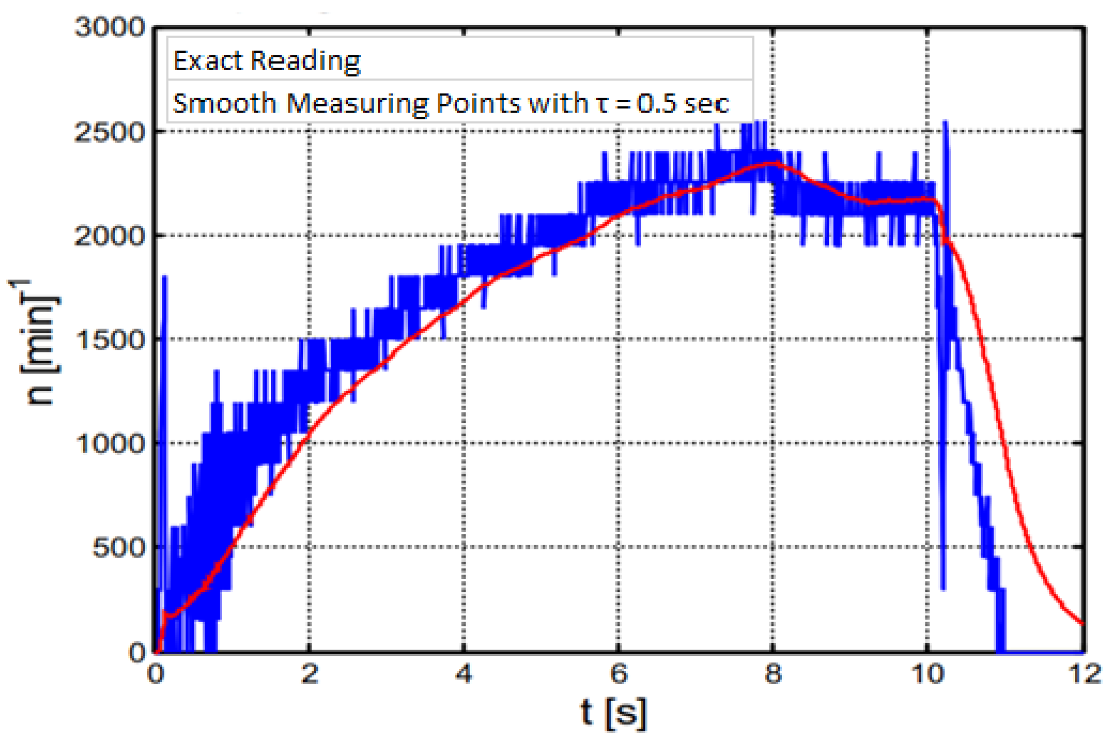
The robot chassis used herein is the RC truck company HPI Savage 2.1 [49]. This truck was fitted into the original equipment using a synchronous motor with a continuous output of about one kilowatt. However, as it had already been used in previous projects, this robot had undergone a few changes to the chassis, and the engine, through the brush DC motor TruckPuller2 7.2 V with 25 W output power, had been replaced. Therefore, a holder was made via which the motor was attached to the chassis. Using a gear with over a fourteen teeth, with module 1, the motor can exercise its power for the robot’s transmission. The reason for conversion is the easy controllability of the new engine at slow speeds. The original engine is designed for speeds up to 100 km/h. Slow movement with this synchronous motor is not essential for a mobile robot. However, it is clear that the new brushed motor is not far-reaching; its rated speed is 6500 revolutions per minute. The chassis offers so much resistance that the motor runs at a rated voltage of slightly more than 2000 revolutions per minute. It also does not reach the rated torque. In general, it can also barely create the engine in which to put the chassis without additional load on the straight and smooth surfaces in motion. Sometimes, however, something becomes stuck, so even the transmission does not succeed. The acceleration and deceleration of the robot using the TruckPuller2 7.2 V engine, with no additional load to the maximum speed as the step response, is shown in Figure 4. Here, the engine speeds were recorded with an incremental encoder, and the unit turns per minute were converted.
The diagram shows the encoder from the real measured values in blue. The quantization of the measured values is very pronounced. The red curve represents the measured values after having smoothed by a PT1 element with a time constant of 0.5 s. The manipulated variable, i.e., the motor’s input voltage, is not shown here. Ideally, the motor plate would turn on when the battery voltage was 7.2 V.
After 10 s, the voltage was switched off again. Unfortunately, even the recording of the step response of the discharged battery was quite strong. Therefore, the speed bowed to pressure at t = 8 s. However, other measurements showed a maximum speed of about 2300 revolutions per minute. Additionally, the slope of the step response in this recording corresponded to that of the other measurements.
There is still a very important factor to evaluate. Shortly after switching, the control variable is single, as seen in both cases as a clear peak in the measured values. It results from a game involving the gear and the connected mechanical power transmission components. The engine accelerates from a standstill, but the backlash is over. The information stored in the motor shaft rotational energy is abruptly transferred to the transmission at the moment the transmission is grabbed. With this setback, the robot is in motion and slowed down, and the drive motor is strong. However, transferring the bulk of the energy into the mass-spring-damper system of the bone and tires, the robot oscillates back, although not properly set off. This strong non-linearity, of course, complicates the controller’s design in terms of speed control.
After the digression on the shortcomings of the robot’s drive, a solution was reached and the problems were markedly reduced. In any case, the engine can be changed. Since brushless motors are available only for high speeds, either a transmission needs to be constructed or stronger and more brushed motors need to be installed. However, two additional brush motors were used, since having complete information is not trivial. It seems likely that the next, larger model of TruckPullers, namely the TruckPuller3 12 V, will have a speed of 6300 min−1 and a torque of 361 Nm, i.e., a 58% higher torque.

3.3. Steering

The existing steering system of the robot is suboptimal in many ways. Firstly, the steering linkage has a mechanical protection system called a servo saver, which protects the servo motor from excessive torque if the wheels are steered abruptly by an external force—for example, when the robot moves obliquely at high speed against a wall. The steering forces applied to the robot at low speeds were so great that these were recorded almost exclusively from this backup and did not extend to the edges. This resulted in driving in this state being almost impossible. In terms of the other needs, the steering servo HiTec HS-5745MG [13] was very powerful. The blocking current in the servo sheet varied from 4 to 4.8 A. In tests, it was shown that in the short term, the servo motor at 5 V supply voltage with fast back and forth movements certainly consumed more than 4 A. However, as it was originally built off the voltage regulator at higher currents than 4 A, it can ensure that the servo motor does not work properly with energy. A large electrolytic capacitor remedied a small issue in the supply branch. However, this is not always enough, so a new voltage regulator is needed.
Unfortunately, a direct connection of the servo motor to a battery of elimination which has since been reported on various Internet forums will hurt less than the maximum supply voltage of six volts to the servo motor. Therefore, this voltage regulator was specially developed. The setting of the servo saver is quite simple. To obtain the screw, however, some covers and brackets were removed. Then, the screw of the servo saver was turned until the spring was maximally stretched, allowing the complete compression of the spring. The servo saver was disabled, and the servo’s power was transmitted to the steering and vice versa. However, there was no longer a protective effect preventing the servo from excessive forces.

3.4. Modeling and Algorithms

This section develops and designs system control modeling for various control elements.

3.4.1. Digital PT1-Element

For smoothing input and state variables, including the sensors’ readings, a PT1 element was used. Since this smoothing was to be implemented in software, a digital representation was required, and it was derived. The starting point is a continuous PT1 element, as shown in Figure 5. Figure 5a represents the input and output behavior of the PT1 element, which is part of Figure 5b, and describes how it works using an integrator and two amplifiers.
First, the differential equation of the PT1 element is established as the right signal flow diagram. The inner signal x 1 t is calculated via the feedback:
x 1 t = u t 1 τ · x 2 t .
At the same time, however, the inner signal x 1 t is the derivative of the inner signal x 2 t .
x 1 t = d x 2 t d t
Now, equating the two Equations (25) and (26), we obtain:
d x 2 t d t = u t 1 τ · x 2 t .
The relationship between the inner signal x 2 t and the output signal y t is
x 2 t = τ · y   differentiating
d x 2 t d t = τ · d y d t .
Inserting this into Equation (27), we obtain:
τ · d y t d t = u t τ τ · y t .
The required differential equation of the continuous PT1 element results from normalization:
d y t d t + 1 τ · y t = u t τ .
It must now be discretized in time. For this purpose, the signals are sampled equi-temporally at times t k ,   k = 0 ,   1 ,   2 , etc. The differentials become differences, with only d y t represented as a difference. The differential d t becomes the time increment Δt. Thus, the following arises:
y k y k 1 Δ t + 1 τ · y k = u k τ .
By solving this equation for y k , ywe obtain:
y k = τ · y k 1 + Δ t · u k τ + Δ t .
If one assumes a structure-invariant PT1 element, this equation can be continued:
y k = a · y k 1 + b · u k
with the constants
a = τ τ + Δ t
and
b = Δ t τ + Δ t
If the constants are stored in memory, the calculation of the PT1 element requires only two multiplications and one addition in a single step. Another advantage of this formula is that due to its simplicity, it is also well suited for integer calculations with suitable normalization.

3.4.2. Digital PID Controller with Anti-Wind-Up Return

A quasi-continuous digital PID controller with first-order anti-wind-up feedback was developed. With the manipulated variable u t as the controller, the output is severely limited. Any limitations in the controlled system are not taken into account. Figure 6 shows the signal flow diagram of the continuous controller with anti-wind-up feedback.
u ¯ t = K p · e t + K i · 0 t e t + a t d t + K d · d e t d t
The manipulated variable error a t is the difference between the unlimited u t and the limited manipulated variable u t , multiplied by the K a w u feedback factor.
a t = K a w u · u t u ¯ t
Inserted into Equation (37), the result is
u ¯ t = K p · e t + K i · 0 t e t + K a w u · u t u ¯ t d t + K d · d e t d t .
This differential equation was then converted into a difference equation with the equi-temporal sampling period T . It was sampled at the points in time t k = k T , with k = 0 ,   1 ,   2 ,   etc. Here, the integral became a sum, whereby all values from the beginning up to the value of the last iteration were summed up.
0 t d t T · i = 0 k 1
The current iteration must not be included in the summation. Otherwise, its values would depend on this formula, and the formula would become transcendental. The difference equation is now
u ¯ k = K p · e k + K i · T · i = 0 k 1 e i + K a w u · u i u ¯ i + K d · e k e k 1 T .
The difference Δ u k of the unlimited manipulated variable from times k and k 1 is now considered.
Δ u ¯ k = K p · e k e k 1 + K i · T · i = 0 k 1 e i + K a w u · u i u ¯ i +                                                           K i · T · i = 0 k 2 e i + K a w u · u i u ¯ i + K d · e k e k 1 e k 1 + e k 2 T
The two sums cancel each other almost completely. Only the summand for the iteration step k 1 remains.
Δ u ¯ k = K p · e k e k 1 + K i · T e k 1 + K a w u · u k 1 u ¯ k 1 + K d · e k 2 · e k 1 + e k 2 T
Equation (43) is now sorted according to the sampling values of the control error e i .
Δ u ¯ k = K p + K d T · e k + K i · T K p 2 · K d T · e k 1 + K d T · e k 2 + + K i · T · K a w u · u k 1 u ¯ k 1
The first term of Equation (44) represents a change in the manipulated variable of a classic quasi-continuous digital PID controller. The second term describes the anti-wind-up feedback. In the case of a structure-invariant controller, the values before the control error samples and the manipulated variables merely represent coefficients that can be calculated in advance. This simplifies the equation to
Δ u ¯ k = a · e k + b · e k 1 + c · e k 2 + d · u d i f f k 1
with
a = K p + K d T ,
b = K i · T K p 2 · K d T ,
c = K d T ,
d = K i · T · K a w u
and
u d i f f k 1 = u k 1 u ¯ k 1 .
The current unlimited manipulated variable u k is made up of the addition of the unlimited manipulated variable from the last iteration u k 1 and the current increase in the manipulated variable Δ u k .
u ¯ k = u ¯ k 1 + Δ u ¯ k
If one inserts the increase in the manipulated variable Δ u k , one obtains
u ¯ k = u ¯ k 1 + a · e k + b · e k 1 + c · e k 2 + d · u d i f f k 1 .
To obtain the limited manipulated variable u k , which is also given to the controlled system, the limiter function l i m i t x must be applied to the unlimited manipulated variable u k . In the signal flow, it reads
l i m i t x = { m i n f ü r x < m i n x f ü r m i n x m a x m a x f ü r x > m a x .
The limited manipulated variable i therefore calculated as
u k = l i m i t u ¯ k .

3.4.3. Controller Control Concept

The proposed research work aimed to develop an autonomous mobile robot. For this, it was necessary to gain control over the kinematics of the robot. A total of three control circuits were used for this purpose which regulated the variables drive speed, robot position, and robot orientation. The last two variables can also be summarized under the term robot pose. First, the speed control loop was considered. Figure 7 shows the block diagram of the control loop.
The digital PID controller with anti-wind-up feedback was used here as the controller. The sensor system is an optical incremental rotary encoder that detects the rotational speed of the drive. Since its signal is subject to strong quantization noise, smoothing in the form of a PT1 element was provided in the feedback path. For the controllers, angular velocities and positions were considered because they are measured at the robot’s gearbox. However, a linear relationship was able to convert them into linear velocities and positions. Next came the position control loop, which was superimposed on the speed controller. The position controller’s manipulated variable represented the speed controller’s setpoint. Both controllers together formed a controller cascade. The control loop parameters are given in Table 4.
The most important property of the control loop is that its reference variable is no longer the time, but the distance covered, x. Roughly speaking, this is because a change in orientation is only possible when the robot moves forward or backward. This movement corresponds to a change in the distance traveled. However, since the controller algorithm continued to be executed at equi-temporal time intervals, it was only able to be designed as a PI controller, since a differential component would have led to singularities when the robot was at a standstill. The PI controller was designed as a simple parallel structure with proportional and integral parts. The integrator value had hard upper and lower limits in order to avoid the winding-up effects of an integral part. The equation for the digital controller is
u x k = K p · w ϕ x k + K i · i = 0 k 1 w ϕ x i · x i ,
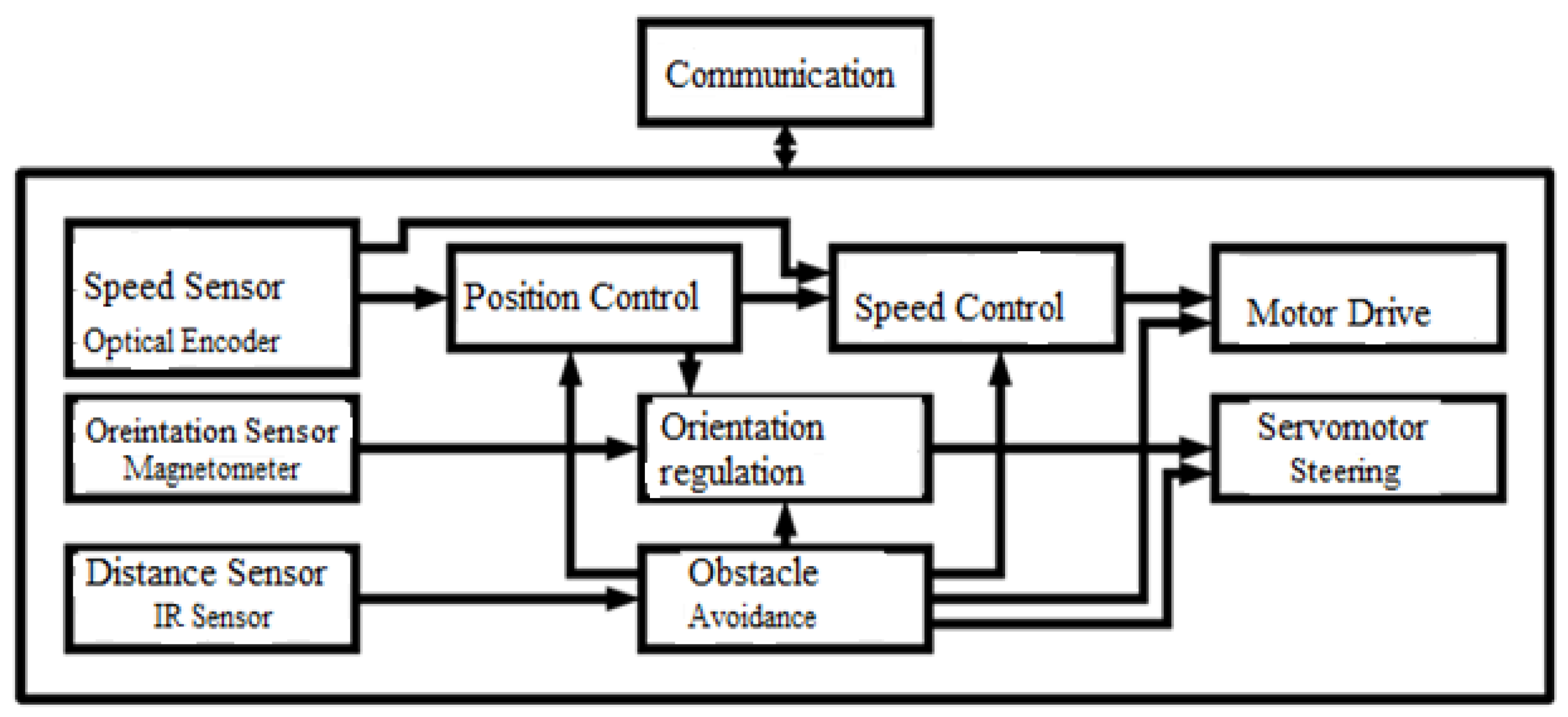
where x k represents the waypoints to be scanned. If the sum exceeded one of the limit values, m i n or m a x , it was limited to the limit value in each run of the sum in which this occurred. The system controlled the robot’s steering, including its subsequent integration, which generated the orientation ϕ from the steering angle θ of the front wheels. A magnetometer served as a sensor system with which the robot’s orientation concerning the Earth’s magnetic field, i.e., the magnetic north pole, was determined. The connections between the controllers are shown in Figure 8.
First, the speed sensor supplied the actual position and speed control values. These two controllers formed a cascade, and the speed controller generated the manipulated variable for the drive. The orientation sensor supplied the actual value for the orientation control. This control also used the target position of the position control to generate the target orientation. The orientation control provided the servomotor for steering. Obstacle avoidance was superimposed on the three controllers, receiving its information from the distance sensors. If an obstacle avoidance event occurred, the position and orientation controllers were switched off, and speed control was supplied using target values for obstacle avoidance. In addition, the obstacle bypass also had direct control over the actuators. The communication via which the controller was connected to a higher level was superimposed on everything.

4. Results and Discussion

4.1. Linearization of the IR Sensor Characteristic Curve

When driving autonomously, the mobile robot must constantly look for obstacles to avoid colliding. Two different types of sensors are used for this purpose: on the one hand, infrared sensors, with each sensor monitoring a very narrow line in space, and on the other hand, ultrasonic sensors, which scan larger spatial cones for obstacles. Our method presents how the characteristic curve of the sensor GP2D12 can be transformed in such a way that there is an almost linear relationship between the sensor’s output voltage and the measured distance. The linearization should be based exclusively on an integer calculation so the microcontroller can quickly process.
First, however, the functionality of the sensor will be briefly explained. The sensor has two lenses arranged side by side. An IR LED is hidden behind one lens, generating a modulated light beam. The lens bundles this light beam, generating a very small light cone. If this beam of light hits an object, it is reflected at a constant angle and returns to the sensor, traversing through the other lens. Behind this lens is a position-sensitive device (PSD), i.e., a single-line camera that detects the position of the light beam on the light-sensitive surface. The PSD, as well as a signal processor integrated with the sensor, convert this position into a voltage. The microcontroller can then measure this voltage.
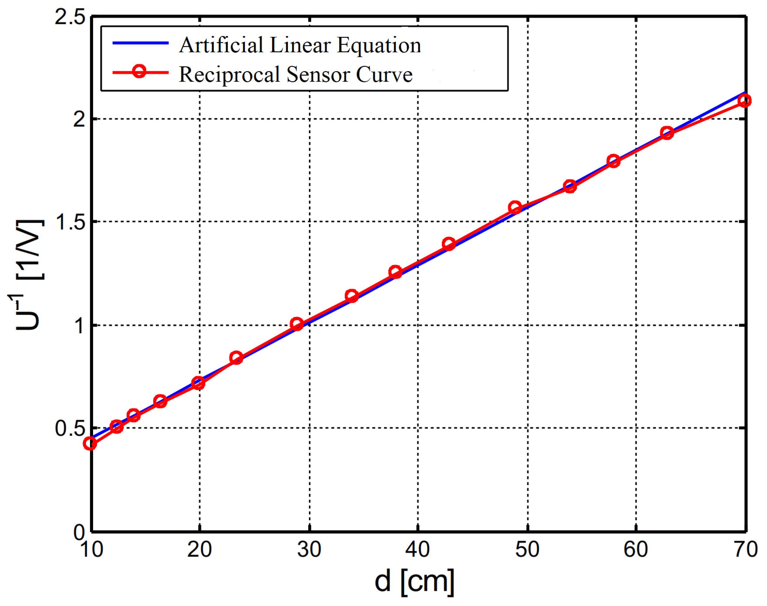
For linearization, an artificial linear Equation (55) was applied, with the distance d as the input variable and the reciprocal voltage U 1 as the output variable. In addition, m represents the slope of the straight line, and b its y-intercept.
U 1 = m · d + b
Using the parameters m and b , the artificial linear Equation (55) must now be brought into congruence with the curve U 1 d obtained from the characteristic curve. A spreadsheet is very well suited for this, since, according to formula (55), the reciprocal voltage U 1 is automatically calculated for the distance points d i and both curves can be displayed simultaneously in one diagram. In this way, the two curves can coincide quickly if the constants m and b are changed.
In the beginning, the U 1 intercept b should be set to zero, and the slope m changed until both lines are parallel. Then, both straight lines can be made to coincide by changing the U 1 axis intercept b .
The selective readout and the simulated straight line are shown in Figure 9. It can be seen that there are hardly any deviations over a large area. The deviations are only slightly larger at the edge areas. The support points ( d i | U i 1 ) of the sensor characteristic read are marked with circles.
Since the voltage U and the distance d are to be determined, Equation (55) is resolved at distance d .
d = U 1 b m
This is the simplest possible form of the equation sought in this study, which can later be calculated using integer numbers. Therefore, all variables and constants are used as little as possible to avoid deviation from the rounded values of their unit digits. The reciprocal voltage, U 1 , is shown again as a fraction, 1 / U , the y-intercept as b = 1 / b 1 , and the slope as m = 1 / m 1 .
This results in
d = 1 U 1 b 1 1 m 1 = m 1 · 1 U 1 b 1 .
Then, the difference in the brackets is written as a fraction bar.
d = m 1 · b 1 U U · b 1
Now, the break can be cleaved in a difference of two fractions. It can break into parts of any size to be reduced.
d = m 1 · b 1 U · b 1 m 1 · U U · b 1 = m 1 U m 1 b 1 = m 1 U b m
The subtrahend to the difference merely represents a constant which can be calculated in advance. It corresponds to an offset of the distance that the sensor always supplies. The sensor voltage in the unit volts was considered. The analog/digital converter of the microcontroller delivered, but the voltage was measured in unit digits, and corresponded to the largest representable digital value of the transducer A D C m a x with the reference voltage V R e f + . The scale of the transducer was linear. Accordingly, the results for the conversion of the voltage U of V in digits were:
U d i g i t s = A D C m a x V R e f + · U V .
Since the distance d is to be issued in centimeters and the original curve was also given in this unit, the length must not be converted. However, the voltage scaling must also be applied to the inverse of the slope m 1 . Thus arises the following:
m d i g i t s · c m 1 = A D C m a x V R e f + · m 1 / V · cm .
Considering the offset b / m , it can be found that this ratio was not adjusted for scaling the voltage, since the scaling of both arguments cancels each other again. Inputting Equations (60) and (61) into Equation (59), after shortening, we obtained:
d cm = m d i g i t s · cm 1 U d i g i t s b 1 / V m 1 / V · cm .
Since this formula is to be calculated only with integer numbers, the constants must be in single digits, with the round function rounded. When divided by the voltage, U is an integer division, i.e., the result is always rounded to the nearest digit, for the floor function. This ultimately results in the removal of integer arithmetic to d :
d cm , I n t e g e r = f l o o r r o u n d m d i g i t s · cm 1 U d i g i t s r o u n d b 1 V m 1 V · cm .
Finally, the formula for the parameters m and b was calculated. Here, the reference voltage of the analog/digital converter V R e f + is assumed to be 2.5 V, and the converter’s resolution to be 10 bits. A resolution of 10 bits results in the largest representable value of the converter being:
A D C m a x = 2 n 1 = 2 10 1 = 1023 .
The inverse slope m d i g i t s · cm 1 can now be calculated from this.
m d i g i t s · cm 1 = A D C m a x V R e f + · m 1 / V · cm = 1023 d i g i t s 2.5 V · 0.028 / V · cm = 14 , 614.29 d i g i t s
Thus, the value rounded to the ones digit is
r o u n d m d i g i t s · cm 1 = 14 , 614 d i g i t s .
Now, the offset is calculated.
b 1 / V m 1 / V · cm = 0.17 / V 0.028 / V · cm = 6.07
The rounded results are:
r o u n d b 1 V m 1 V · cm = 6 .
The function to be implemented in the microcontroller for calculating the measured distance d in centimeters is now:
d cm , I n t e g e r = 14 , 614 d i g i t s U d i g i t s 6 .
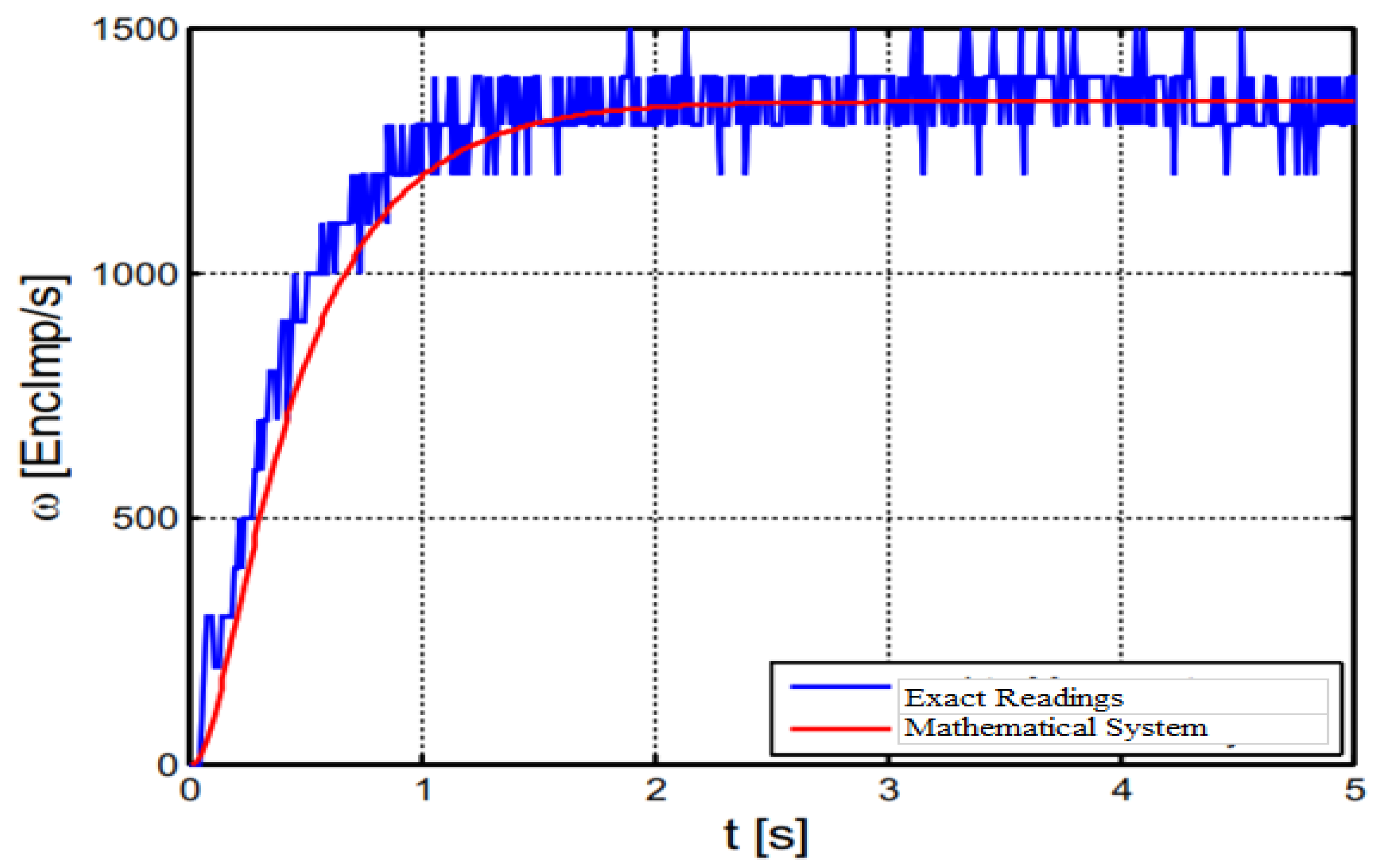
To adjust the control loop, a drive train model that is as precise as possible is required. As already mentioned, the drive is modeled by a PT2 element and a subsequent integrator. The parameters are determined by analyzing the robot’s step response. The distance covered is recorded by the robot as a function of time via the step response function. The step response shown in Figure 10 was carried out with two “TruckPuller3 12 V” drive motors with a battery voltage of 7.2 V and without a mounted PC. The blue characteristic shows the measured values. The quantization by the rotary encoder can be seen very well here. The red characteristic describes an ideal PT2 element with a gain of K S = 1350, and the time constants τ S 1 = 0.1 s and τ S 2 = 0.4 s. This element represents a fairly good approximation of the real system.

4.2. Speed Control Loop

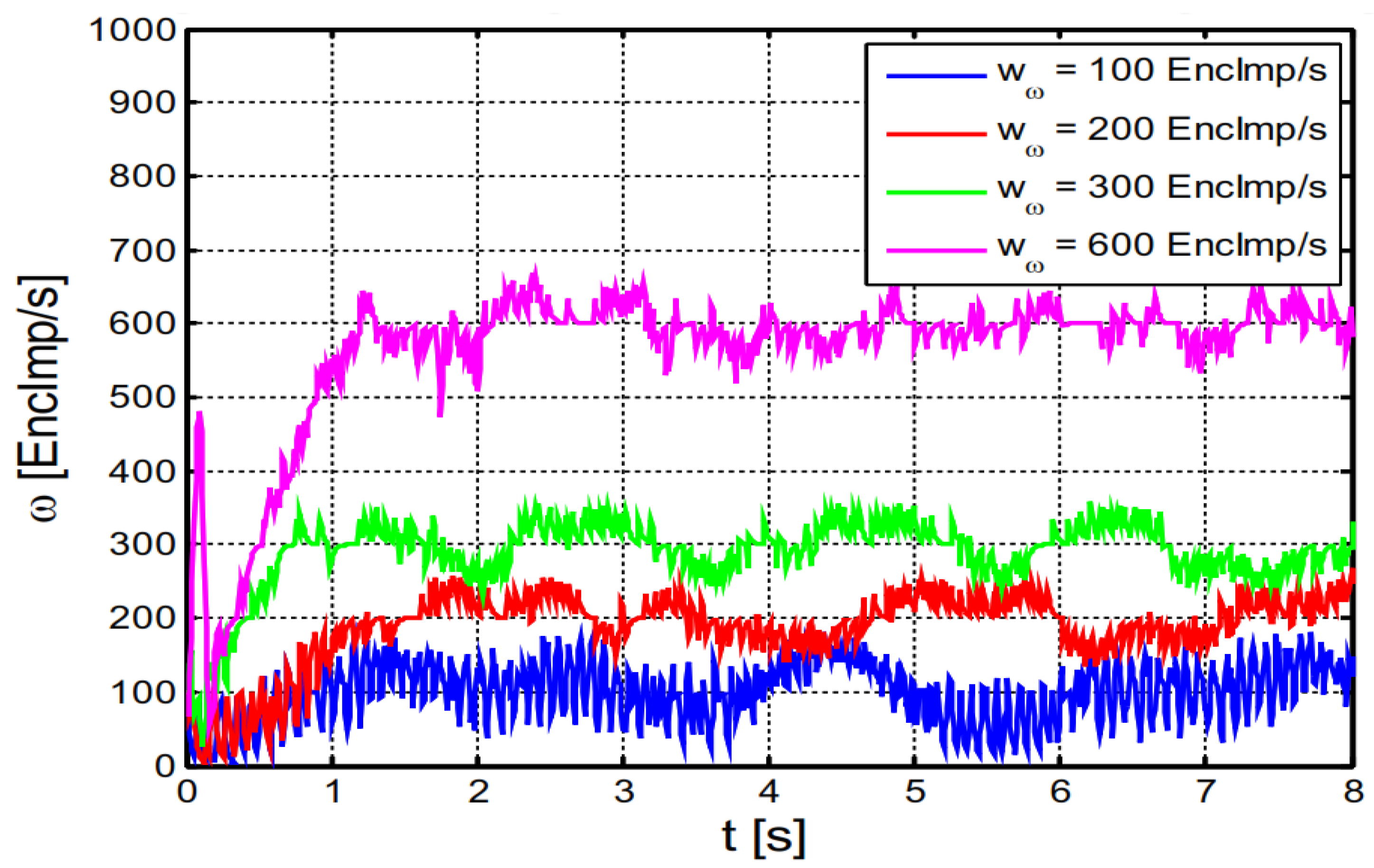
An experiment was conducted to analyze the speed controller. The rotary encoder created a 100 EncImp/s quantization of the actual speed. Different responses (i.e., 100, 200, 300 and 600 EncImp/s) of the closed speed were recorded, as shown in Figure 11. The step responses were recorded in the hallway of the EE building at the University of King Abdul Aziz. It is considered a reference-free environment because the ground is very flat. It is noted from Figure 11 that all step responses reached their final values after about one second, and then oscillated around it. A recorded deviation (i.e., around ±50 EncImp/s) of the slightly smoothed measured values is acceptable. The oscillating behavior probably results from many individual components. The deviation is comparable with the latest results [67,68].

4.3. Orientation Determination Using Magnetometers

This section aims to describe the theory behind determining the absolute orientation of an object using a magnetometer.
Determining the offset error and channel distortion due to the different sensitivities is easy. The magnetometer is rotated once in a circle. The smallest and largest measured values are saved for each channel, and the offset error for each channel is the mean between the minimum and maximum values.
O f f s e t i = B i , m i n + B i , m a x 2   with   i   =   x ,   y
Here, the B i measurements of magnetic field strength are given. The sensitivity correction for the x-channel can be determined from the difference between the minimum and maximum readings. It is given by
D i s t y / x = B y , m a x B y , m i n B x , m a x B x , m i n .
This results, accordingly, in the following corrected measured values:
B x , k o r r = D i s t y / x · B x O f f s e t x
and
B x , k o r r = B y O f f s e t y .
The arctangent-two function can determine the magnetic field direction from these corrected readings.
ϕ = a t a n 2 B y , k o r r , B x , k o r r .
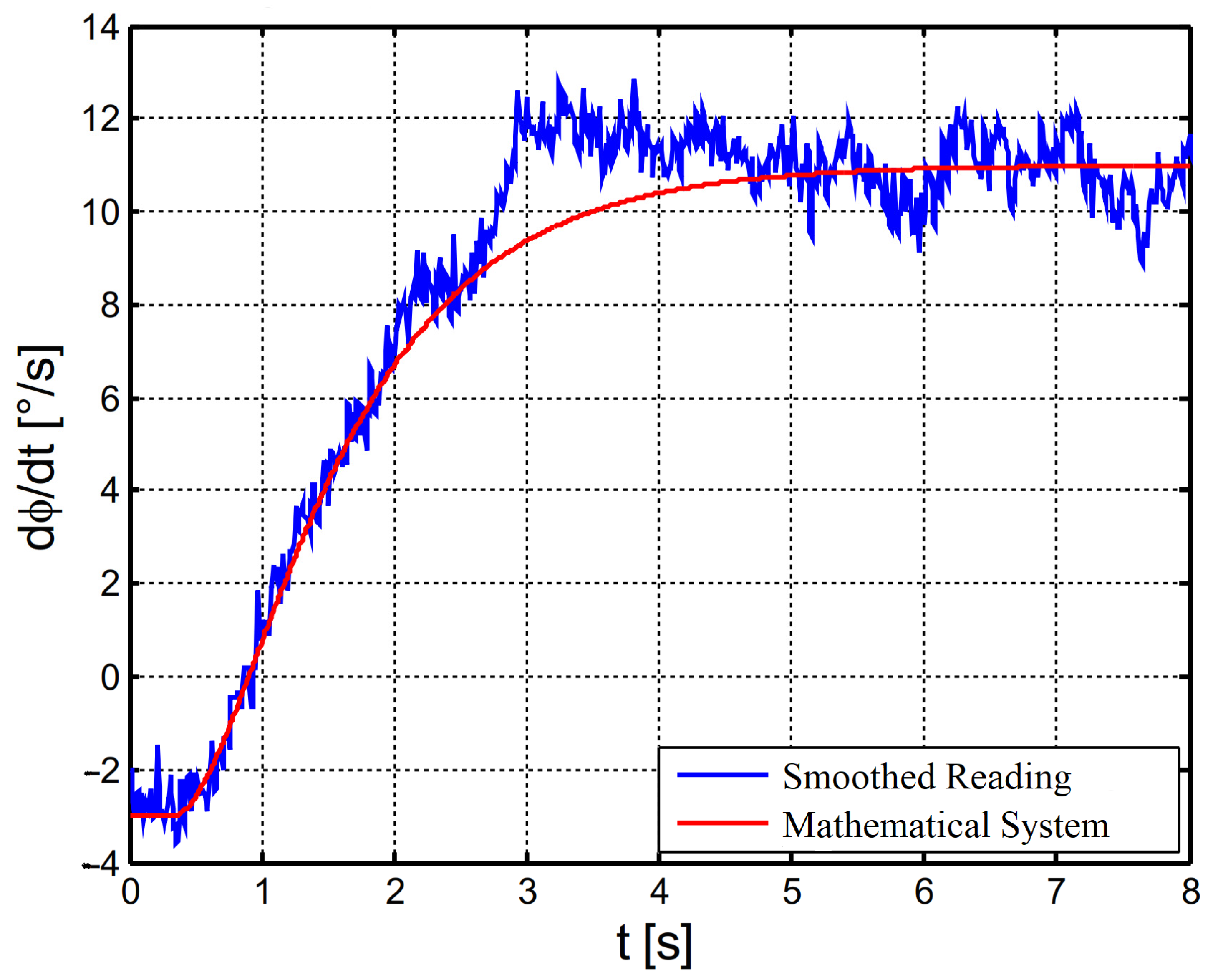
The CPMS09 magnetometer [48] has automatic tilt compensation, which is calculated using the accelerometer. The controller is programmed for a speed of 600 EncImp/s, and the corresponding step response is shown in Figure 12. A relatively large deviation exists between the measured step response and the mathematical model. First, the change in orientation does not start exactly at zero. The robot could not drive in an exact straight line due to the steering play, and it was blocked by metal objects. The magnetic field was slightly distorted. These two factors also explain why the measured amplification of the system of 11° − (−3°) = 14° deviated from the theoretical value of 9.32°. However, the order of magnitude agrees well. The results of the following observation are only guide values and should not be seen as an absolute limit. The orientation controller must be optimized by experimenting nonetheless.

4.4. Self-Localization

In this section, a self-localization test is described. The magnetometer was calibrated before the driving test. To perform the test drive, the robot was driven in both directions, clockwise and counter-clockwise. The flow measurement was recorded to determine the difference in each direction. Then, to capture the complete picture, both trajectories were finally superimposed onto a Google Maps aerial photograph. To visualize the fitness of the trajectories, their sizes were adjusted according to the EE building of the University. The results shown in Figure 13 demonstrate that the aspect ratio and orientation were retained.
The red trajectory, which runs clockwise, was recorded first. It can be seen that the calibration of the magnetometer was very good. The start and end points of the trajectory were the same. It can be seen that the tracks ran fairly parallel to the outline of the building.
An experiment was conducted to compare the proposed approach with the A* algorithm [60]. Various trials were conducted for different durations and at different time periods. The results showed that the proposed approach was better able to cover the distance from the doctor’s office to patient A’s room. The cumulative distance covered by each approach is noted in Table 5.

5. Conclusions

An IoT-enabled telepresence robot is attractive in many application areas of healthcare and industries where physical interaction with patients is impossible. For such situations, human–robot interaction becomes compulsory. A well-controlled robot would be useful for performing tasks in a future pandemic situation. This article’s objective was to provide a stable design for a robot able to move and communicate in a controlled environment. To this end, controlled test drives were undertaken, and the results were evaluated. The settings for the robot were then determined from these. Finally, the ideally adjusted robot was checked for its desired behavior.
Herein, we presented a control theory for the purpose of normalizing the integration process and offering a well-developed robot for the medical sciences. The research problem was developed and empirically tested following the proposed path toward the development of the robot. The results validate the proposed approach’s sustainability and usability, and present a ready robot for short and long-term bioengineering tasks. Our findings showed better results than a default system, particularly when deployed in highly interactive medicine scenarios.

Author Contributions

Conceptualization, A.A.A.; methodology, M.N.K. and M.T.; software, M.N.K.; validation, A.A.A. and M.N.K.; formal analysis, M.N.K.; investigation, M.N.K.; resources, A.A.A.; writing—original draft preparation, M.N.K. and M.T.; writing—review and editing, A.A.A.; supervision, M.N.K. and M.T.; funding acquisition, A.A.A. and M.T. All authors have read and agreed to the published version of the manuscript.

Funding

This work was supported by the Deanship of Scientific Research at Prince Sattam bin Abdulaziz University under the research project (PSAU/2023/01/23001).

Institutional Review Board Statement

Not applicable.

Informed Consent Statement

Not applicable.

Data Availability Statement

Not applicable.

Conflicts of Interest

The authors declare no conflict of interest.

References

  1. Guillén-Climent, S.; Garzo, A.; Muñoz-Alcaraz, M.N.; Casado-Adam, P.; Arcas-Ruiz-Ruano, J.; Mejías-Ruiz, M.; Mayordomo-Riera, F.J. A Usability Study in Patients with Stroke Using MERLIN, a Robotic System Based on Serious Games for Upper Limb Rehabilitation in the Home Setting. J. Neuroeng. Rehabil. 2021, 18, 41. [Google Scholar] [CrossRef] [PubMed]
  2. Alotaibi, Y. Automated Business Process Modelling for Analyzing Sustainable System Requirements Engineering. In Proceedings of the 2020 6th International Conference on Information Management (ICIM), London, UK, 27–29 March 2020; IEEE: Piscataway, NJ, USA, 2020. [Google Scholar] [CrossRef]
  3. Karimi, M.; Roncoli, C.; Alecsandru, C.; Papageorgiou, M. Cooperative Merging Control via Trajectory Optimization in Mixed Vehicular Traffic. Transp. Res. Part C Emerg. Technol. 2020, 116, 102663. [Google Scholar] [CrossRef]
  4. Kitazawa, O.; Kikuchi, T.; Nakashima, M.; Tomita, Y.; Kosugi, H.; Kaneko, T. Development of Power Control Unit for Compact-Class Vehicle. SAE Int. J. Altern. Powertrains 2016, 5, 278–285. [Google Scholar] [CrossRef]
  5. Alotaibi, Y.; Malik, M.N.; Khan, H.H.; Batool, A.; ul Islam, S.; Alsufyani, A.; Alghamdi, S. Suggestion Mining from Opinionated Text of Big Social Media Data. Comput. Mater. Contin. 2021, 68, 3323–3338. [Google Scholar] [CrossRef]
  6. Alotaibi, Y. A New Meta-Heuristics Data Clustering Algorithm Based on Tabu Search and Adaptive Search Memory. Symmetry 2022, 14, 623. [Google Scholar] [CrossRef]
  7. Rodríguez-Lera, F.J.; Matellán-Olivera, V.; Conde-González, M.Á.; Martín-Rico, F. HiMoP: A Three-Component Architecture to Create More Human-Acceptable Social-Assistive Robots. Cogn. Process. 2018, 19, 233–244. [Google Scholar] [CrossRef]
  8. Anuradha, D.; Subramani, N.; Khalaf, O.I.; Alotaibi, Y.; Alghamdi, S.; Rajagopal, M. Chaotic Search-And-Rescue-Optimization-Based Multi-Hop Data Transmission Protocol for Underwater Wireless Sensor Networks. Sensors 2022, 22, 2867. [Google Scholar] [CrossRef]
  9. Laengle, T.; Lueth, T.C.; Rembold, U.; Woern, H. A Distributed Control Architecture for Autonomous Mobile Robots-Implementation of the Karlsruhe Multi-Agent Robot Architecture (KAMARA). Adv. Robot. 1997, 12, 411–431. [Google Scholar] [CrossRef]
  10. Lakshmanna, K.; Subramani, N.; Alotaibi, Y.; Alghamdi, S.; Khalafand, O.I.; Nanda, A.K. Improved Metaheuristic-Driven Energy-Aware Cluster-Based Routing Scheme for IoT-Assisted Wireless Sensor Networks. Sustainability 2022, 14, 7712. [Google Scholar] [CrossRef]
  11. Atsuzawa, K.; Nilwong, S.; Hossain, D.; Kaneko, S.; Capi, G. Robot Navigation in Outdoor Environments Using Odometry and Convolutional Neural Network. In Proceedings of the IEEJ International Workshop on Sensing, Actuation, Motion Control, and Optimization (SAMCON), Chiba, Japan, 4–6 March 2019. [Google Scholar]
  12. Nagappan, K.; Rajendran, S.; Alotaibi, Y. Trust Aware Multi-Objective Metaheuristic Optimization Based Secure Route Planning Technique for Cluster Based IIoT Environment. IEEE Access 2022, 10, 112686–112694. [Google Scholar] [CrossRef]
  13. Subahi, A.F.; Khalaf, O.I.; Alotaibi, Y.; Natarajan, R.; Mahadev, N.; Ramesh, T. Modified Self-Adaptive Bayesian Algorithm for Smart Heart Disease Prediction in IoT System. Sustainability 2022, 14, 14208. [Google Scholar] [CrossRef]
  14. Anavatti, S.G.; Francis, S.L.; Garratt, M. Path-Planning Modules for Autonomous Vehicles: Current Status and Challenges. In Proceedings of the 2015 International Conference on Advanced Mechatronics, Intelligent Manufacture, and Industrial Automation (ICAMIMIA), Surabaya, Indonesia, 15–17 October 2015; IEEE: Piscataway, NJ, USA, 2015; pp. 205–214. [Google Scholar]
  15. Rae, I.; Venolia, G.; Tang, J.C.; Molnar, D. A framework for understanding and designing telepresence. In Proceedings of the 18th ACM Conference on Computer Supported Cooperative Work & Social Computing, Vancouver, WA, Canada, 14–18 March 2015; pp. 1552–1566. [Google Scholar]
  16. Tuli, T.B.; Terefe, T.O.; Rashid, M.U. Telepresence mobile robots design and control for social interaction. Int. J. Soc. Robot. 2020, 13, 877–886. [Google Scholar] [CrossRef] [PubMed]
  17. Alami, R.; Chatila, R.; Fleury, S.; Ghallab, M.; Ingrand, F. An Architecture for Autonomy. Int. J. Robot. Res. 1998, 17, 315–337. [Google Scholar] [CrossRef]
  18. Hitec HS-5745MG Servo Specifications and Reviews. Available online: https://servodatabase.com/servo/hitec/hs-5745mg (accessed on 28 November 2022).
  19. Optical Encoder M101|MEGATRON. Available online: https://www.megatron.de/en/products/optical-encoders/optoelectronic-encoder-m101.html (accessed on 28 November 2022).
  20. Singh, S.P.; Alotaibi, Y.; Kumar, G.; Rawat, S.S. Intelligent Adaptive Optimisation Method for Enhancement of Information Security in IoT-Enabled Environments. Sustainability 2022, 14, 13635. [Google Scholar] [CrossRef]
  21. Kress, R.L.; Hamel, W.R.; Murray, P.; Bills, K. Control Strategies for Teleoperated Internet Assembly. IEEE/ASME Trans. Mechatron. 2001, 6, 410–416. [Google Scholar] [CrossRef]
  22. Goldberg, K.; Siegwart, R. Beyond Webcams: An Introduction to Online Robots; MIT Press: Cambridge, MA, USA, 2002; ISBN 0-262-07225-4. [Google Scholar]
  23. Brito, C.G. Desenvolvimento de Um Sistema de Localização Para Robôs Móveis Baseado Em Filtragem Bayesiana Não-Linear. 2017. Available online: https://bdm.unb.br/bitstream/10483/19285/1/2017_CamilaGoncalvesdeBrito.pdf (accessed on 3 February 2023).
  24. Rozevink, S.G.; van der Sluis, C.K.; Garzo, A.; Keller, T.; Hijmans, J.M. HoMEcare ARm RehabiLItatioN (MERLIN): Telerehabilitation Using an Unactuated Device Based on Serious Games Improves the Upper Limb Function in Chronic Stroke. J. NeuroEngineering Rehabil. 2021, 18, 48. [Google Scholar] [CrossRef] [PubMed]
  25. Schilling, K. Tele-Maintenance of Industrial Transport Robots. IFAC Proc. Vol. 2002, 35, 139–142. [Google Scholar] [CrossRef] [Green Version]
  26. Srilakshmi, U.; Alghamdi, S.A.; Vuyyuru, V.A.; Veeraiah, N.; Alotaibi, Y. A Secure Optimization Routing Algorithm for Mobile Ad Hoc Networks. EEE Access 2022, 10, 14260–14269. [Google Scholar] [CrossRef]
  27. Sennan, S.; Kirubasri; Alotaibi, Y.; Pandey, D.; Alghamdi, S. EACR-LEACH: Energy-Aware Cluster-Based Routing Protocol for WSN Based IoT. Comput. Mater. Contin. 2022, 72, 2159–2174. (accessed on 29 April 2022). [Google Scholar] [CrossRef]
  28. Ahmad, A.; Babar, M.A. Software Architectures for Robotic Systems: A Systematic Mapping Study. J. Syst. Softw. 2016, 122, 16–39. [Google Scholar] [CrossRef] [Green Version]
  29. Sharma, O.; Sahoo, N.C.; Puhan, N.B. Recent Advances in Motion and Behavior Planning Techniques for Software Architecture of Autonomous Vehicles: A State-of-the-Art Survey. Eng. Appl. Artif. Intell. 2021, 101, 104211. [Google Scholar] [CrossRef]
  30. Ziegler, J.; Werling, M.; Schroder, J. Navigating Car-like Robots in Unstructured Environments Using an Obstacle Sensitive Cost Function. In Proceedings of the 2008 IEEE Intelligent Vehicles Symposium, Eindhoven, The Netherlands, 4–6 June 2008; IEEE: Piscataway, NJ, USA, 2008; pp. 787–791. [Google Scholar]
  31. González-Santamarta, M.Á.; Rodríguez-Lera, F.J.; Álvarez-Aparicio, C.; Guerrero-Higueras, Á.M.; Fernández-Llamas, C. MERLIN a Cognitive Architecture for Service Robots. Appl. Sci. 2020, 10, 5989. [Google Scholar] [CrossRef]
  32. Shao, J.; Xie, G.; Yu, J.; Wang, L. Leader-Following Formation Control of Multiple Mobile Robots. In Proceedings of the 2005 IEEE International Symposium on, Mediterrean Conference on Control and Automation Intelligent Control, Limassol, Cyprus, 27–29 June 2005; IEEE: Piscataway, NJ, USA, 2005; pp. 808–813. [Google Scholar]
  33. Faisal, M.; Hedjar, R.; Al Sulaiman, M.; Al-Mutib, K. Fuzzy Logic Navigation and Obstacle Avoidance by a Mobile Robot in an Unknown Dynamic Environment. Int. J. Adv. Robot. Syst. 2013, 10, 37. [Google Scholar] [CrossRef]
  34. Favarò, F.; Eurich, S.; Nader, N. Autonomous Vehicles’ Disengagements: Trends, Triggers, and Regulatory Limitations. Accid. Anal. Prev. 2018, 110, 136–148. [Google Scholar] [CrossRef]
  35. Gopalswamy, S.; Rathinam, S. Infrastructure Enabled Autonomy: A Distributed Intelligence Architecture for Autonomous Vehicles. In Proceedings of the 2018 IEEE Intelligent Vehicles Symposium (IV), Suzhou, China, 26–30 June 2018; IEEE: Piscataway, NJ, USA, 2018; pp. 986–992. [Google Scholar]
  36. Allen, J.F. Towards a General Theory of Action and Time. Artif. Intell. 1984, 23, 123–154. [Google Scholar] [CrossRef]
  37. Hu, H.; Brady, J.M.; Grothusen, J.; Li, F.; Probert, P.J. LICAs: A Modular Architecture for Intelligent Control of Mobile Robots. In Proceedings of the Proceedings 1995 IEEE/RSJ International Conference on Intelligent Robots and Systems. Human Robot Interaction and Cooperative Robots, Pittsburgh, PA, USA, 5–9 August 1995; IEEE: Piscataway, NJ, USA, 1995; Volume 1, pp. 471–476. [Google Scholar]
  38. Alami, R.; Chatila, R.; Espiau, B. Designing an Intelligent Control Architecture for Autonomous Robots; ICAR: New Delhi, India, 1993; Volume 93, pp. 435–440. [Google Scholar]
  39. Khan, M.N.; Hasnain, S.K.; Jamil, M.; Imran, A. Electronic Signals and Systems: Analysis, Design and Applications; River Publishers: Gistrup, Denmark, 2022. [Google Scholar]
  40. Kang, J.-M.; Chun, C.-J.; Kim, I.-M.; Kim, D.I. Channel Tracking for Wireless Energy Transfer: A Deep Recurrent Neural Network Approach. arXiv 2018, arXiv:1812.02986. [Google Scholar]
  41. Zhao, W.; Gao, Y.; Ji, T.; Wan, X.; Ye, F.; Bai, G. Deep Temporal Convolutional Networks for Short-Term Traffic Flow Forecasting. IEEE Access 2019, 7, 114496–114507. [Google Scholar] [CrossRef]
  42. Schilling, K.J.; Vernet, M.P. Remotely Controlled Experiments with Mobile Robots. In Proceedings of the Thirty-Fourth Southeastern Symposium on System Theory (Cat. No. 02EX540), Huntsville, AL, USA, 19 March 2002; IEEE: Piscataway, NJ, USA, 2002; pp. 71–74. [Google Scholar]
  43. Moon, T.-K.; Kuc, T.-Y. An Integrated Intelligent Control Architecture for Mobile Robot Navigation within Sensor Network Environment. In Proceedings of the 2004 IEEE/RSJ International Conference on Intelligent Robots and Systems (IROS)(IEEE Cat. No. 04CH37566), Sendai, Japan, 28 September–2 October 2004; IEEE: Piscataway, NJ, USA, 2004; Volume 1, pp. 565–570. [Google Scholar]
  44. Lefèvre, S.; Vasquez, D.; Laugier, C. A Survey on Motion Prediction and Risk Assessment for Intelligent Vehicles. Robomech J. 2014, 1, 1. [Google Scholar] [CrossRef] [Green Version]
  45. Behere, S.; Törngren, M. A Functional Architecture for Autonomous Driving. In Proceedings of the First International Workshop on Automotive Software Architecture, Montreal, QC, Canada, 4–8 May 2015; pp. 3–10. [Google Scholar]
  46. Carvalho, A.; Lefévre, S.; Schildbach, G.; Kong, J.; Borrelli, F. Automated Driving: The Role of Forecasts and Uncertainty—A Control Perspective. Eur. J. Control. 2015, 24, 14–32. [Google Scholar] [CrossRef] [Green Version]
  47. Liu, P.; Paden, B.; Ozguner, U. Model Predictive Trajectory Optimization and Tracking for On-Road Autonomous Vehicles. In Proceedings of the 2018 21st International Conference on Intelligent Transportation Systems (ITSC), Maui, HI, USA, 4–7 November 2018; IEEE: Piscataway, NJ, USA, 2018; pp. 3692–3697. [Google Scholar]
  48. Weiskircher, T.; Wang, Q.; Ayalew, B. Predictive Guidance and Control Framework for (Semi-) Autonomous Vehicles in Public Traffic. IEEE Trans. Control. Syst. Technol. 2017, 25, 2034–2046. [Google Scholar] [CrossRef]
  49. Zhou, X.; Xu, P.; Lee, F.C. A Novel Current-Sharing Control Technique for Low-Voltage High-Current Voltage Regulator Module Applications. IEEE Trans. Power Electron. 2000, 15, 1153–1162. [Google Scholar] [CrossRef]
  50. Gil, A.; Segura, J.; Temme, N.M. Numerical Methods for Special Functions; SIAM: Philadelphia, PA, USA, 2007; ISBN 0-89871-634-9. [Google Scholar]
  51. Milla, K.; Kish, S. A Low-Cost Microprocessor and Infrared Sensor System for Automating Water Infiltration Measurements. Comput. Electron. Agric. 2006, 53, 122–129. [Google Scholar] [CrossRef]
  52. Microchip Technology Inc. DSPIC33FJ32MC302-I/SO-16-Bit DSC, 28LD,32KB Flash, Motor, DMA,40 MIPS, NanoWatt-Allied Electronics & Automation, Part of RS Group. Available online: https://www.alliedelec.com/product/microchip-technology-inc-/dspic33fj32mc302-i-so/70047032/?gclid=Cj0KCQiA1ZGcBhCoARIsAGQ0kkqp_8dGIbQH-bCsv1_OMKGCqwJWGl9an18jsfWWs9DhtuKKYZec_aoaAheKEALw_wcB&gclsrc=aw.ds (accessed on 28 November 2022).
  53. #835 RTR Savage 25. Available online: https://www.hpiracing.com/en/kit/835 (accessed on 28 November 2022).
  54. Types of Magnetometers-Technical Articles. Available online: https://www.allaboutcircuits.com/technical-articles/types-of-magnetometers/ (accessed on 28 November 2022).
  55. Zhu, H.; Brito, B.; Alonso-Mora, J. Decentralized probabilistic multi-robot collision avoidance using buffered uncertainty-aware Voronoi cells. Auton. Robot. 2022, 46, 401–420. [Google Scholar] [CrossRef]
  56. Batmaz, A.U.; Maiero, J.; Kruijff, E.; Riecke, B.E.; Neustaedter, C.; Stuerzlinger, W. How automatic speed control based on distance affects user behaviours in telepresence robot navigation within dense conference-like environments. PLoS ONE 2020, 15, e0242078. [Google Scholar] [CrossRef] [PubMed]
  57. Xia, P.; McSweeney, K.; Wen, F.; Song, Z.; Krieg, M.; Li, S.; Du, E.J. Virtual Telepresence for the Future of ROV Teleoperations: Opportunities and Challenges. In Proceedings of the SNAME 27th Offshore Symposium, Houston, TX, USA, 22 February 2022. [Google Scholar]
  58. Dong, Y.; Pei, M.; Zhang, L.; Xu, B.; Wu, Y.; Jia, Y. Stitching videos from a fisheye lens camera and a wide-angle lens camera for telepresence robots. Int. J. Soc. Robot. 2022, 14, 733–745. [Google Scholar] [CrossRef]
  59. Fiorini, L.; Sorrentino, A.; Pistolesi, M.; Becchimanzi, C.; Tosi, F.; Cavallo, F. Living With a Telepresence Robot: Results From a Field-Trial. IEEE Robot. Autom. Lett. 2022, 7, 5405–5412. [Google Scholar] [CrossRef]
  60. Wang, H.; Lou, S.; Jing, J.; Wang, Y.; Liu, W.; Liu, T. The EBS-A* algorithm: An improved A* algorithm for path planning. PLoS ONE 2022, 17, e0263841. [Google Scholar] [CrossRef]
  61. Howard, T.M.; Green, C.J.; Kelly, A.; Ferguson, D. Statespace sampling of feasible motions for high-performance mobile robotnavigation in complex environments. J. Field Robot. 2008, 25, 325–345. [Google Scholar] [CrossRef]
  62. Wang, S. State Lattice-Based Motion Planning for Autonomous on-Roaddriving. PhD Thesis, Freie University, Berlin, Germany, 2015. [Google Scholar]
  63. Likhachev, M.; Ferguson, D.; Gordon, G.; Stentz, A.; Thrun, S. Any-time search in dynamic graphs. Artif. Intell. 2008, 172, 1613–1643. [Google Scholar] [CrossRef] [Green Version]
  64. Brezak, M.; Petrovi, I. Real-time approximation of clothoids withbounded error for path planning applications. IEEE Trans. Robot. 2014, 30, 507–515. [Google Scholar] [CrossRef]
  65. Lim, W.; Lee, S.; Sunwoo, M.; Jo, K. Hierarchical trajectoryplanning of an autonomous car based on the integration of a samplingand an optimization method. IEEE Trans. Intell. Transp. Syst. 2018, 19, 613–626. [Google Scholar] [CrossRef]
  66. Silver, D.; Lever, G.; Heess, N.; Degris, T.; Wierstra, D.; Riedmiller, M. Deterministic policy gradient algorithms. In Proceedings of the 31st International Conference on Machine Learning, Beijing, China, 21–26 June 2014. [Google Scholar]
  67. Naseer, F.; Khan, M.N.; Altalbe, A. Telepresence Robot with DRL Assisted Delay Compensation in IoT-Enabled Sustainable Healthcare Environment. Sustainability 2023, 15, 3585. [Google Scholar] [CrossRef]
  68. Schouten, A.P.; Portegies, T.C.; Withuis, I.; Willemsen, L.M.; Mazerant-Dubois, K. Robomorphism: Examining the effects of telepresence robots on between-student cooperation. Comput. Hum. Behav. 2022, 126, 1069800. [Google Scholar] [CrossRef]
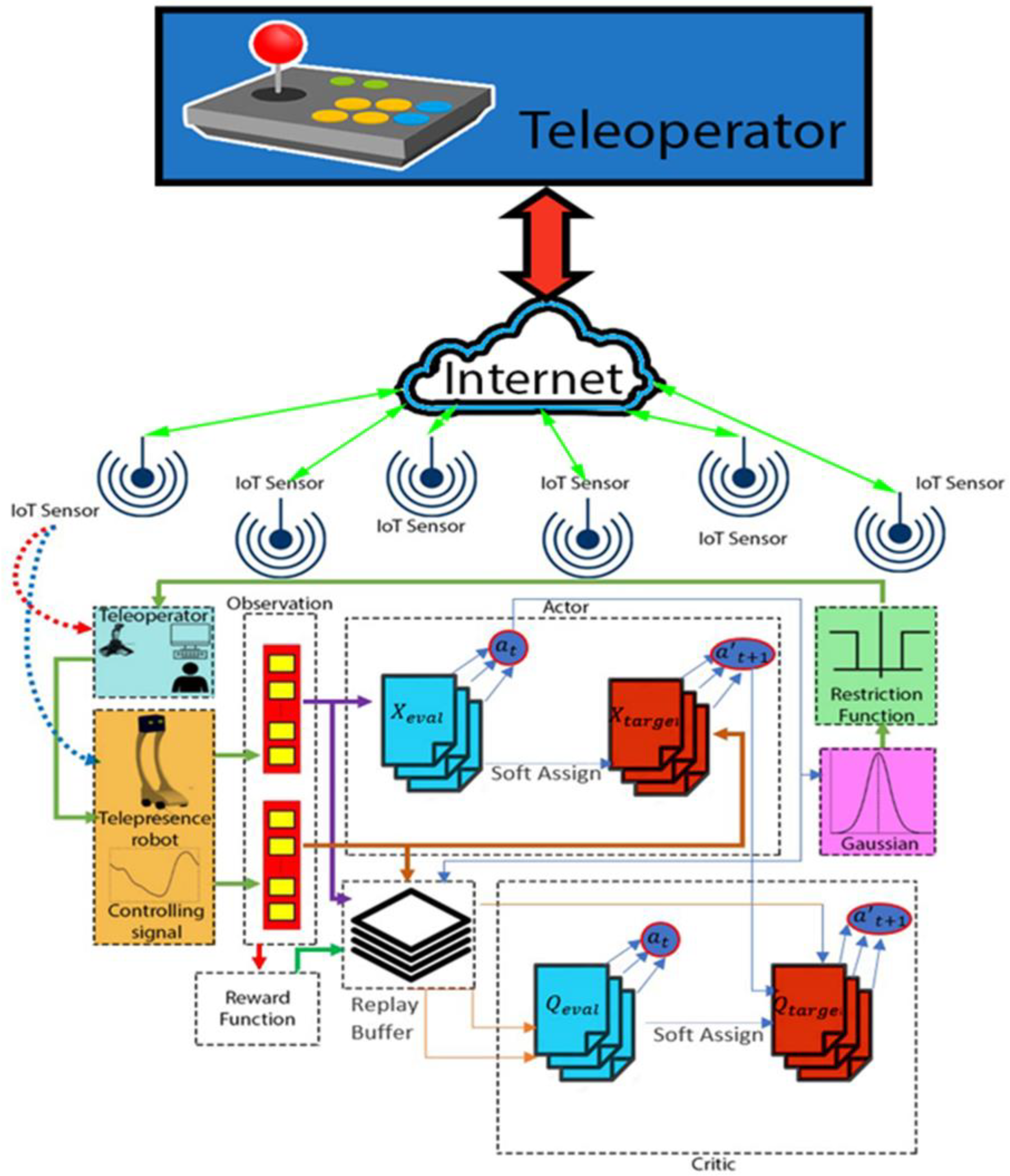
Figure 1. A generalized block diagram with telepresence robot attachment [59].
Sustainability 15 05692 g001
Figure 2. Structure diagram: sensor–actuator control.
Sustainability 15 05692 g002
Figure 3. (a) Voltage divider and filter composed of resistor and capacitor. (b) Input filter of an analog input measuring voltage.
Sustainability 15 05692 g003
Figure 4. Step response of the actuator of the robot with a 7.2 v TruckPuller2.
Sustainability 15 05692 g004
Figure 5. (a) Input and output behavior of the PT1 element. (b) Working on PT1 using an integrator and two amplifiers.
Sustainability 15 05692 g005
Figure 6. PID controller with anti-wind-up return.
Sustainability 15 05692 g006
Figure 7. Control concept of the speed controller.
Sustainability 15 05692 g007
Figure 8. Relationships between the controllers, including sensors and actuators.
Sustainability 15 05692 g008
Figure 9. Linearization of the characteristic curve of the sensor GP2D12.
Sustainability 15 05692 g009
Figure 10. The step response speed of the robot.
Sustainability 15 05692 g010
Figure 11. Different step responses of the closed speed controller.
Sustainability 15 05692 g011
Figure 12. Step response of the orientation controller with a steering value step from 0 to 75.
Sustainability 15 05692 g012
Figure 13. Self-localization results from Google Maps.
Sustainability 15 05692 g013
Table 1. Telepresence robot parameters.
ParametersUnitValue
Obstacles3 × 3 feet9 (fixed)
TrackCoiled1
Initial Point-Doctor’s Office
Termination Point-Patient Ward
Total Distance Meters130
Table 2. Different approaches with limitations.
AuthorsApproachesLimitations
T. M. Howard [61]This approach creates sensitive search spaces which showadditional benefits over existing approaches when steering in diverse paths. It digitizess the stroke and state space, and transforms the original control problem into a graph search problem, which permits the use of pre-computed motion.Utilizing this approach, it is easy to satisfy the environmental constraints when the planned trajectories are expressed in state space, but their dynamic probability cannot be easily guaranteed. It also requires a high amount of computational power.
S Wang [62]This approach utilizes the state lattice for the trajectories and chooses the optimum constraint based on the cost criteria. In this approach, it is simpler producing reasonable paths using the motion planner.This approach increases the chances of unnecessary shorts in a spatial horizon. For optimum work, it is recommended that a non-uniform sampling of the spatial horizon should be used to construct the state lattice.
M. Likhachev [63]Authors in this approach present an algorithm which solves the constrained sub-optimality.It requires superior a priori modelling of the environment. If the models are not precise, the algorithms give inaccurare results, which is also not recommended in a dynamic environment.
M. Brezak [64]This approach interpolates lines and circles, and conducts the path investigation over the continuous trajectory planning.The obtained results are not optimal, and the trajectories are not smooth.
W. Lim [65]These approaches implement numerical optimization, which is an extension of sampling and interpolation.Due to the additional optimization step, thecomplexity increases, and this approach not recommended for real-time applications in this case.
David Silver [66]Authors demonstrate a deterministic policy gradient algorithm with continuous actions.The implementation of this approach can result in rough-moving behavior. The cost function derivation becomes complex. It is also not recommended in an environment of moving obstacles.
F Naseer [67]The deep reinforcement learning (DRL)-based deep deterministic policy gradient (DDPG) enhances control over the TR in case of connectivity issues. It also suggests a proper approach to maneuver the TR in unknown scenarios.This method needs further enhancement in case of dynamic obstacles and further improvement for multi-robotic tasks. Its performance is worse in cases of moving obstacles and disconnectivity.
Table 3. Measurement of the internal resistance of the GP2D12 sensor.
R L a s t U R L a s t I U R i R i
2.5 kΩ1.119 V447.6 µA32 mV71.5 Ω
1 kΩ1.070 V1.07 mA81 mV75.7 Ω
Table 4. Position controller parameters.
ParameterSignificance
K d Gain of the differential component of the PID controller
K p Gain of the proportional component of the PID controller
K i Amplification of the integral component of the PID controller
K a w u Strengthening the anti-wind-up return
m i n The lower limit of the manipulated variable
m a x The upper limit of the manipulated variable
τ The time constant of the smoothing in the feedback branch in seconds
MaxErrValue in encoder pulses differentiate the target’s actual position from the target position. The robot’s actual position is at the end of a Teiltrajektorie in the interval [−MaxErr target position, target position MaxErr+], so the goal is reached and the robot is stopped.
MaxSpeedMaximum average speed in EncImp/Cyc at which the robot should accelerate
AccelAcceleration of the robot in EncImp/Cyc2
Table 5. Comparison of A* with the proposed approach.
AlgorithmsExamplesTrial 1Trial 2Trial 3Mean
Distance (m)/Time(s)Distance (m)/Time(s)Distance (m)/Time(s)Distance (m)/Time(s)
A*First trip8.85 m/91 s9.79 m/99 s9.15 m/95 s9.25 m/95 s
Second trip9.95 m/90 s9.15 m/87 s8.15 m/88 s9.10 m/88 s
Proposed FrameworkFirst trip8.15 m/84 s8.85 m/89 s7.75 m/85 s8.25 m/86 s
Second trip7.85 m/86 s7.55 m/87 s8.15 m/88 s7.85 m/87 s
Disclaimer/Publisher’s Note: The statements, opinions and data contained in all publications are solely those of the individual author(s) and contributor(s) and not of MDPI and/or the editor(s). MDPI and/or the editor(s) disclaim responsibility for any injury to people or property resulting from any ideas, methods, instructions or products referred to in the content.