Article

An Artificial-Intelligence-Based Renewable Energy Prediction Program for Demand-Side Management in Smart Grids

by
Vinothini Arumugham
1,*,
Hayder M. A. Ghanimi
2,
Denis A. Pustokhin
3,
Irina V. Pustokhina
4,
Vidya Sagar Ponnam
5,
Meshal Alharbi
6,
Parkavi Krishnamoorthy
1 and
Sudhakar Sengan
7
1
School of Computer Science and Engineering, Vellore Institute of Technology, Chennai 600127, Tamil Nadu, India
2
Biomedical Engineering Department, College of Engineering, University of Warith Al-Anbiyaa, Karbala 56001, Iraq
3
Department of Logistics, State University of Management, 109542 Moscow, Russia
4
Department of Entrepreneurship and Logistics, Plekhanov Russian University of Economics, 117997 Moscow, Russia
5
Department of Computer Science and Engineering, Koneru Lakshmaiah Education Foundation, Vaddeswaram 522302, Andhra Pradesh, India
6
Department of Computer Science, College of Computer Engineering and Sciences, Prince Sattam Bin Abdulaziz University, Alkharj 11942, Saudi Arabia
7
Department of Computer Science and Engineering, PSN College of Engineering and Technology, Tirunelveli 627152, Tamil Nadu, India
*
Author to whom correspondence should be addressed.
Sustainability 2023, 15(6), 5453; https://doi.org/10.3390/su15065453
Submission received: 14 February 2023 / Revised: 16 March 2023 / Accepted: 17 March 2023 / Published: 20 March 2023
(This article belongs to the Special Issue Security Issues in the Research and Application of Renewable Energy)

Abstract

:
Technology advancements have enabled the capture of Renewable Energy Sources (RES) on a massive scale. Smart Grids (SGs) that combine conventional and RES are predicted as a sustainable method of power generation. Moreover, environmental conditions impact all RES, causing changes in the amount of electricity produced by these sources. Furthermore, availability is dependent on daily or annual cycles. Although smart meters allow real-time demand prediction, precise models that predict the electricity produced by RES are also required. Prediction Models (PMs) accurately guarantee grid stability, efficient scheduling, and energy management. For example, the SG must be smoothly transformed into the conventional energy source for that time and guarantee that the electricity generated meets the predicted demand if the model predicts a period of Renewable Energy (RE) loss. The literature also suggests scheduling methods for demand-supply matching and different learning-based PMs for sources of RE using open data sources. This paper developed a model that accurately replicates a microgrid, predicts demand and supply, seamlessly schedules power delivery to meet demand, and gives actionable insights into the SG system’s operation. Furthermore, this work develops the Demand Response Program (DRP) using improved incentive-based payment as cost suggestion packages. The test results are valued in different cases for optimizing operating costs through the multi-objective ant colony optimization algorithm (MOACO) with and without the input of the DRP.

1. Introduction

Because of increased awareness of Energy Consumption (EC) and production worldwide, the market share of renewable sources has been increasing. Renewable Energy Sources (RES) are predicted to outperform fossil fuels in monthly power generation. There is a departure from the industry’s restraint and unsustainable resources, and consumers and energy providers have developed using 23% green power. However, the infrastructure operations are complicated, and utility companies and consumers are challenged due to the inconsistency of market demand and supply of extensive energy that RES and utility companies and consumers can meet. The energy company applied Smart Grid (SG) technology to stabilise the Green Energy Supply (GES) and make RE trustworthy and future-proof.
A traditional Distribution System (DS) supports the energy flow from suppliers to users. Energy transmission and distribution with SGs are performed using a SG as a one-way electrical interconnection system integrated with massive production points as the only energy source at multiple locations. The industries require multiple extra production points combined with the increased volume of smaller RE generation plants. The new paradigm could not be continued by the conventional method, which depends on the operator-enabled power system, and highly flexible operation management is allowed because a SG solution replaces it.
Future SG-based DSs will also be able to meet the increased use of renewable Wave Swell Energy (WSE) sources that behave in a standard method that repeats itself. The operation’s security may be endangered due to this [1]. There is a need for Advanced Measuring Infrastructure (AMI) [2] to guarantee the cost-efficient and secure operation of these systems and to use cutting-edge design for Distributed Energy Resources (DER) [3,4]. AMI provides smart meters, which have the features of remote control, monitoring, and readability, by creating bidirectional telecommunication between electricity companies and customers, embracing data collection and transmission by energy providers, information analysis and processing, and implementing EC management to ensure system reliability and balance supply and demand [5,6]. Since the environmental impact is reduced, the market situation, reliability, and service should be enhanced. An SG will incorporate information and Communications Technology (ICT) into each component, such as electricity generation, EC, and delivery. An SG makes the seamless integration of unreliable RES and the potential for efficient power distribution and delivery highly possible. The scale of SG adoption is the basis for efficiently incorporating RE into the energy sector, supporting technologies such as smart meters and the Internet of Things (IoT), and big data will drive it forward. While deploying RE systems, control is a complex aspect. For super-performance and reliable operations, WSE is required. By implementing digitally enabled SGs, such as the IoT, consumers and energy suppliers will be provided with advanced tools for monitoring and regulating SG performance. It is performed by controlling multiple devices at production points and households.
Vast IoT infrastructures are supported by adopting SG devices and facilitating leveraging skills for digital risk protection. There is more adaptability of the network to oversupplies or electricity shortages that the RES has in common with a conventional model integrated with grid-connected devices. The resource computer and the smart devices are connected, and the essential information is collected to cope with electricity usage and help stabilize the whole grid. Utility companies advance their operations by carefully analysing the data collected in the SG network. Data associated with operational device status, quality of power, self-test, smart meter, and consumption level are collected by advanced metering infrastructure.
Few data are considered for real-time processing due to edge computing and 5G adoption. Profound knowledge of performance skills, enhanced performance, and consumer behaviour is enhanced using big data. Energy providers enhance SG optimization and more customer engagement, along with data analytics. RES especially encourages the application of big data and predictive analytics. Because of it is unpredictability, sustainable electricity demands reasonable efforts due to its instability to incorporate it into the energy network based on homogeneous fuel. The suppliers can project energy generation and EC rates, mitigate risks, and make constructive decisions based on the processed data.
With the help of big data analytics, utility companies can improve the efficiency of SG based on how they use real-time data or how well they collected data in the past—continuous monitoring systems and improved energy production and distribution work to address the current challenges simultaneously. For the SG, it is predicted that the latest hike in variable wind and generation of SP will boost more Renewable Energy (RE) shares in the future in the cumulative generation portfolio, and challenges related to SG management make the task of predicting WP essential for the SG. The relevant balancing actions are getting more complicated, leading to greater variable WSE penetration.
The existing applicable methods’ inventory, including data from the meteorological department and power system, and disseminating this data, which requires the communication structure, are essential. The obtaining of accurate information that requires PMs, such as software and data, and the need for infrastructure to generate and communicate this information are included in the proposed model.
The unsureness in the behaviour of WSE is one of the significant demerits in RES management. Network operators always use energy storage local services to control manufacture shortages and balance EC and production before using WSE and the rest of the REs in the power system. Now, storage and finding a solution for solving this unsureness are more mandatory than ever with the emergence of WSE and the absence of certainty in production capabilities. Demand Response Program (DRP) usage is one of these solutions [7].
Recently, by conducting studies to implement better Demand-Side Management Programs (DSMP) and roles, a balance has been formed between EC and RE generation. A WSR-based SG is managed using a DRP [8]. To ignore the use of the pollution emission function to model the micro-grid management, the resolution for the proposed model is made through the Particle Swam Optimization (PSO) algorithm. To mitigate the cost of functioning and emissions, in [9], the evaluation of multi-objective operation planning in a SG distribution with WSR was performed as a probabilistic model; in Wind Power (WP) and Solar Power (SP), the variations are modelled with the help of Probability Density Functions (PDFs). This reference does not consider the corresponding generation of SP and WP modelling. On the other hand, there is an omission from the pollution function’s definition for elements such as Sulphur Dioxide (SO2) or Nitrogen Oxides (NOx) and for problem-solving the three-constraint method is used. Reference [10] discussed the same type of issue, which was solved using the scenario tree method; the researchers in this study ignored the SP modelling.
In the Mesh Adaptive Direct Search Method (MSDSM), the generation of RE that causes uncertainty was ignored [11]. A single objective function changes a multi-objective function, and a method called Mixed Integer Programming (MILP) is used to resolve the recommended method. To increase social welfare, [12] studied the DSMP in an SG’s application, assuming the generation of WP, i.e., a WPP and the improbability it caused. The authors do not consider the benefits of SP generation, and the incentive-based DRP, which motivates customers to participate, is not used in this research. In [13], the Monte-Carlo-Method-Based Stochastic Planning Approach (MCMBSPA) was suggested to model the wind and Demand Response (DR) stochastic behaviour in an energy market after considering the WP’s impact as operational storage.
To develop the DRP, the authors of [14] used incentive-based payments as cost-suggested packages. The simulation results are reviewed in three separate instances to optimize operating costs and productions with and without DR. Users in an SG-connected microgrid with energy storage used an independent and distributive DSMP based on Bayesian Game Theory (BGT) designed by [15]. Each user’s EC of shiftable loads is modelled as a noncooperative III-players game with partial data in which all users compete compared with the storage element and all other microgrid users.
A new method [16] has been developed for reducing residual demand to improve the mix and spatial distribution of WP and PV capacity in Europe. Micro-Grid Energy Management (MGEM) is described as mixed-integer linear programming [17] and presents a new multi-objective solution and DRP. DR is included in the optimization challenge to prove its impact on energy dispatch and their technological and commercial benefits.
A stochastic optimization framework for DR with dynamic pricing and Plug-in Electric Vehicles (PEVs) is by [18]. This paper proposes a stochastic optimization framework for demand response that considers dynamic pricing and PEVs. The limitations of this work are that it does not consider uncertainties in the energy stock market and the PEV charging behaviour. The proposed model in [19] is a dynamic Zonal Congestion Management (ZCM) model based on the DRP. The model uses power tracing techniques and sensitivity analysis to determine the congestion control zones based on an introduced Congestion Index (CI) that considers both the effectiveness of congestion alleviation and the responsibility for congestion creation. The proposed model does not consider integrating RE sources, which can impact congestion management in the long run as the distribution of RE in the energy mix increases.
Further, the model assumes that the system operator has perfect information about the power system, which may not always be true in practice. Inaccurate information can lead to ineffective congestion management.
An “Integrated Energy Management System (EMS) for Microgrids of building prosumers” was proposed by [20]. A microgrid EMS for building prosumers is the proposed design. It reduces microgrid operation costs for buildings, RES, ESS, and PEVs. However, the proposed EMS does not consider uncertainties in the energy market, such as fluctuating energy costs and unpredictable weather patterns that affect RE generation. Although the proposed optimization problem is designed to minimize a microgrids’ operation cost, it is unclear whether it can be scaled to larger microgrids or distribution networks. An optimal EMS for microgrids considering ESS, DR, and RE generation was proposed by [21]. The paper proposes a scenario-based EMS model for microgrids (MGs) in stand-alone mode that utilizes ESSs and demand-side flexibility to ensure autonomous power supply while maintaining stability. The potential limitation of this study is that it assumes perfect information, which may not be realistic in real-world scenarios. The study focuses on reducing network energy losses but does not consider other principal factors, such as environmental impacts or economic feasibility.
This paper optimizes the smart grid’s WP, SP prediction, and DRP to minimize energy costs and emissions. WP and SP prediction were tested using cutting-edge Deep Learning (DL) models. Further, the proposed DRP is implemented to base the DRP method on an incentive, as the participation of consumers in these programs is deemed voluntary. To provide DR packages, such as cost and storage, for commercial, industrial, and residential consumers based on their situations, consumers select one of the presented packages and contribute to a DRP. The Water Surface Pressure Gradient (WSPG) is modelled using Rayleigh and the beta Probability Density Function (PDF) proposed in this paper. Considering the fuzzy-mechanism-based Pareto criterion in integration with nonlinear sorting, the Multi-Objective Ant Colony Optimization (MOACO) method is used to optimize the DRP.
The paper is structured as follows: Section 2 presents the predictions of SP and WP generation, Section 3 presents the MOACO-based DRP model, Section 4 presents the result and discussion, and Section 5 concludes the work.

2. RES Prediction

2.1. Solar Power Prediction (SPP)

The model is initialized by integrating Numerical Weather Predictions (NWP) to start with an ideal stage. Weather satellites and ground weather stations provide these weather predictions. Because of huge-scale forces, the predicted weather modifications, such as SP, speed, and clouds, can be assessed using standard operational NWP models at national centres. However, the prediction of WP or SP resources, adapted to the WP or SP plant’s particular application and the WP or SP plant’s location, is permitted by personalized NWP. A chance to assimilate exclusive local observations at the neighbouring power plant is provided. NWP models vary in the model grid’s resolution and spatial model domain. The model grid’s conventional spatial resolutions of 50 km for the global and approximately 2 km for the region are integrated with the global PM, i.e., globally and regionally, with an area-restricted MESO scale to operate. Well-designed global PMs forecast large-scale synoptic weather patterns. However, with less than 10 km of horizontal resolution, the regional models’ current role is overtaken by the persistent hike in computer power.
NWP approaches have been introduced based on the application and related time scale. The short-term time scale, from minutes up to a few hours, has adequate time series models that use on-site measurements. The ground-based sky imagers are used to acquire high spatial and temporal resolution that enables intra-hour prediction. Cloud motion vectors from satellite-image-based forecasts show a reliable performance for the next 30 min to the next 6 h. Photovoltaic (PV)-SG requires a prediction of up to 2 days. The NWP models are the basis of this prediction.
This section provides the basic ideas and information needed to understand and make solar power predictions. Primary factors such as SP monitoring, performance assessment metrics, and solar PMs that need general inputs are used to measure the performance of predictions.

2.1.1. Components and Applications of Irradiance

With a difference of less than 0.1% per year [22], there is 1.36 kWm2 of extraterrestrial SP at the top of the atmosphere. How good a variable value depends on the local weather and where it is in ground-level SP. Global Horizontal Irradiance (GHI) is the absolute solar power that hits a horizontal ground surface. The GHI’s are classified as Diffuse Irradiance and Direct Normal Irradiance (DNI), where the energy from the ground level usually comes from the solar beam and contains a small volume of circumsolar energy [23]. Diffuse Horizontal Irradiance (DFI) energy propagates through the atmosphere. Equation (1)
HI = DNIcos θ z + DIF
The association between DNI, GHI, and DFI is where the solar zenith angle is θ z and the solar elevation angle θ e θ z + θ e = 90 is the balancing angle. DNI develops more sensitivity towards atmospheric cloud covers and aerosol concentrations when compared with GHI. For example, the DNI is dropped by moving clouds in a few seconds from hundreds of W m2 to 0 [24].
There is a considerable correlation between operational PV generation and GH. As a result, the increasing development of PV capacity has motivated future research on GHI resourcing and prediction. Alternatively, the real-time tracking of the SP results only in using DNI components by the Concentrated Solar Power (CSP) technologies. Thus, a powerful desire for researching and predicting DNI resourcing is stimulated by the latest increase in the development of global CSP systems.
The future power result, or SP, is the result of the solar PMs. This is the difference in the value of the PMs between models and choosing the values needed to make a PM. The following are the inputs commonly used in intra-hour solar prediction applications: local weather data, sky image features, and historical and current energy data.

2.1.2. Measured Irradiance Data

Solar PMs’ endogenous inputs and training targets represent clear-sky indices and irradiance measurements. The literature uses temporal resolutions of 1 to 5 min combined with lagged 30 to 60 min data for intra-hour forecast horizons. However, this is not enough for the solar ramps’ accurate prediction (caused by evolving clouds) to be performed by solar PM containing just endogenous inputs [25]. To the PM, there is a necessity for exogenous inputs to be predicted since they are important for plant management, operations of rapid distribution, and enabling inverter control by the solar ramp [26]. The accuracy that SP expects in predicting solar ramp measures is enhanced by exogenous inputs such as cloud cover information and weather data provided by sky images [27].

2.1.3. Meteorological Data

Table 1 contains the meteorological variables commonly used for deploying the intra-hour solar prediction. The meteorological data are received from the weather stations of neighbouring or local NWPs. In situ observations are chosen because they have a high temporal resolution. In the absence of in situ observations, high-resolution time series of NWP data from NWP are interpolated as global inputs [28]. Data normalization, a commonly used and effective method, improves the sturdiness and standardisation of data-driven models [29]. Data are normalized by increasing the certainty of NWP data, improving data stability, and simplifying object-to-data mapping. The Min–Max scaling score normalization method is frequently used to normalize the meteorological data in the solar prediction domain. The definition of Min–Max feature scaling normalization is as follows: Equation (2):
X normalized   = X X min X max X min
where a weather variable’s value is X, set the data at the MIN and MAX as X min ,   X max . The definition of the standard value of normalization is as follows: Equation (3)
X normalized   = X μ σ ,
where X’s mean and standard deviations are ‘m’ and ‘s’.

2.1.4. Local Sky Imaging Data

The use of cloud indices provided by NWPs every 6 to 12 h is permitted for intra-day and day-ahead solar prediction. However, to be used for intra-hour solar prediction, this is not sufficient [30]. So, sky imagers—the local sensing systems—provide information related to ground-detected clouds in integration with greater temporal and spatial resolution. Relevant studies obtain summarized statical features from sky images as exogenous inputs because millions of pixels are checked in a high-resolution sky image. Feature Extraction (FE) is performed using statistical RGB analysis or cloud detection methods. A complete sky image (FE) is presented in [31]. However, these image-based FE methods that minimise installation and transfer costs are usually performed manually.

2.1.5. Mathematical Modelling

The prediction problem is as follows: a time of historical climate data is given x 1 ;   x 2   .   .   .   x n and the number of weather inputs is represented by “n”. The following is a mapping function “f” between future solar PV and historical weather data defined to forecast day-ahead solar PV by Equation (4).
y ^ = f x 1 , x 2 , x n
The solar PV-PM with n = 6 weather inputs’ is shown in Figure 1.
As PV panels become more affordable, utilities are increasingly installing high potentials at Solar Power Plants (SPPs); later, the output power is regulated via an inverter to satisfy the guidelines of maximum capacity, commonly referred to as curtailment. However, especially during the winter, the day’s maximum power output mismatches with the sun’s position due to curtailment. As a result, in our work, the target values do not match the precise amount of energy generated by PV panels, which are more closely related to the sun’s location throughout the year. However, the target values include the power outputs of a regulated SPP that fails to track the sun’s position very precisely. This work assessed the optimal power generation curve daily for the inverter effect. We defined “ideally” as the volume of SPP electricity output generated in exceptionally sunny weather with no cloud cover but with curtailment.
Due to the extensive data, the true daily pattern is difficult to observe. On the other hand, the greatest values of the blue “lines” represent the highest daily power generation, which varies seasonally and monthly. Additionally, the red cosine of the sun’s zenith angle showed that maximum power outages would not occur daily. The monthly optimum condition of the day is defined in this work, i.e., the output of the optimum day’s power was determined for each month based on a historical day’s sample, wherein a set of circumstances contained the energy output.
SPP per day and hour can be the value of the daily sum and the monthly maximum sum s d , m = h P h d , m . A similar quantity for daily_max S m = M a x s d , m and monthly daily_max is computed as: m d , m = M a x ( P h d , m   and   M m = M a x m d , m .
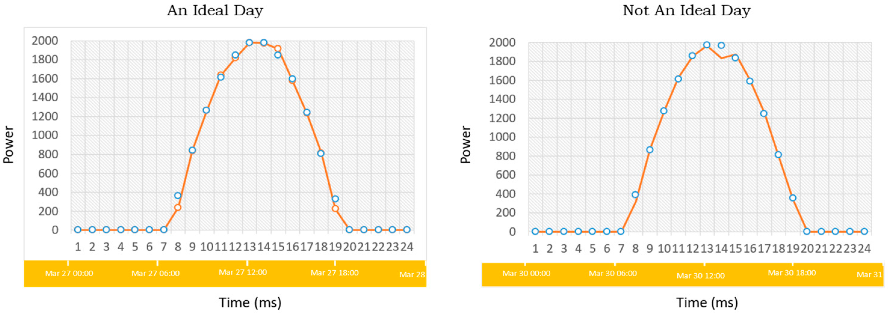
Algorithm 1 depicts the algorithm for selecting ideal days from historical data. To summarize, optimal days would have a daily sum and high output of more than enough compared with all previous days in that month. In addition, the optimum day will possess a smooth bell curve with no abrupt decrease in power production. Figure 2 depicts an ideal and a non-ideal day.
Algorithm 1 Ideal Days Selection Algorithm
Step 1: Initialize m 0 ,   d 0 , h 5   ;
Step 2: While d d m Do
Step 3: While m 12 do:
Step 4: I   S m × 0.9   ;
Step 5: J   M m × 0.95 ;
Step 6: If s d . m < I Then
Step 7: Ideal:= False;
Step 8: Else If m d . m < J Then
Step 9: Ideal:= False;
Step 10: Else
Step 11: While h 19 do:
Step 12: P   a v g p h 1 d , m , p h + 1 d , m × 0.9 ;
Step 13: If p h 1 d , m < P Then
Step 14: Ideal:= False;
Step 15: Break;
Step 16: Else If p h 1 d , m P < 200 Then
Step 17: Ideal:= False;
Step 18: Break;
Step 19: Else
Step 20: Ideal:= True;
Step 21: End If;
Step 22: End Do;
Step 23: End If;
Step 24: End Do;
Step 24: End Do;
Step 25: End
This work computes the “distance” or “similarity” between the actual and ideal power outputs. To summarize the method, for every training day, similarity metrics are determined. Next, the cumulative summary statistics of such a day’s weather are used for training a Support Vector Regression (SVR) model, which tends to forecast the similarity metrics at the time of forecast. The hourly SP output is then predicted using the predictable similarity metrics and hourly weather data.

2.1.6. Deep Learning Models

The weather condition’s temporal evolution is distributed, and its impact on SP output is investigated using the Temporal Convolutional Network (TCN)-based DL method proposed in this study. Each day has a set time, ranging from 5 a.m. to 8 p.m. for 16 h. On an hourly basis, the target SP output is measured, so each day contains 16 target values. Several methods exist for extending the network’s connectivity in the time dimension, which investigates the weather data’s spatiotemporal dimensions daily.
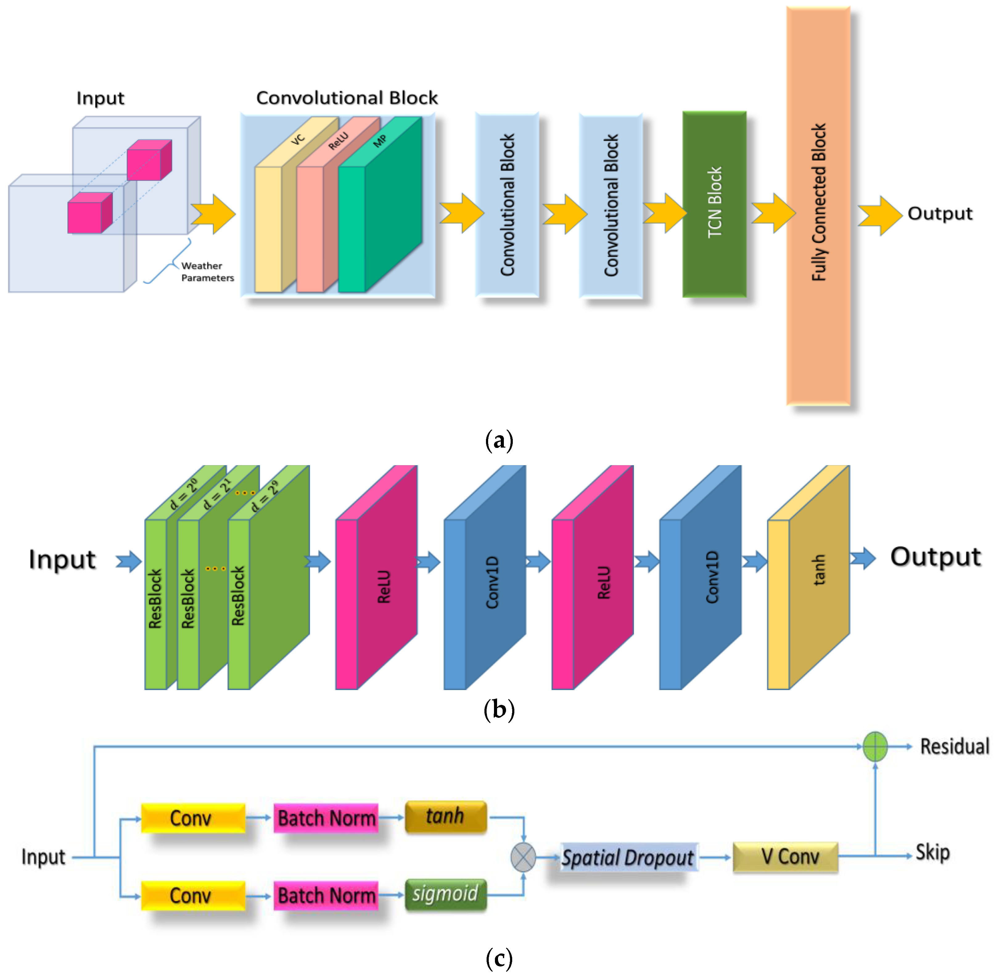
On the temporal dimension, connectivity is accomplished in phases. Figure 2 shows three temporal connection patterns evaluated: a single hour, a daily, and a hybrid model. With a weather-grid-data-based 4D tensor, the single-hour model solely considers inter-hour temporal connectedness. The daily model with NWP data assumes a 4D tensor containing NWP data for the previous 16 h and an output equivalent to 16 hourly solar outputs.
  • Single-Hour Model
The winning models and the tested networks are like the winning models in the ImageNet challenge: AlexNet and ResNet. This model deployed the TCN combined with the Volumetric Convolution Neural Network (VCNN) layer instead of the spatial convolution layer. On a multi-dimensional input tensor built with different weather inputs, a 4D convolution is applied by a volumetric convolution layer followed by TCN. The spatial dimensions in spatial convolution are where convolutions are exclusively applied. A 3D filter is convoluted to perform convolutions from the spatial and temporal dimensions in 4D-CNNs to extract spatial–temporal relation information automatically. The VCNN and TCN-based Neural Networks (NN) are depicted in Figure 3a–c. Throughout the temporal and spatial dimensions, the derived features are accessible to heterogeneous channels containing information about the weather using VCNN. As a result, it can recognise cloud movement patterns, which influence SP outputs.
The formal name for a unit’s value at location (t, x, y) is inside the feature map (i, j) with a layer v i j t x y , Equation (5).
v i j t x y = ReLU b i j + m r = 0 R i 1 p = 0 P i 1 q = 0 Q i 1 w i j m r p q v i 1 m t + r x + p y = q
where the Rectified Linear Unit is ReLU, which allows only definite outputs to be transmitted over the network, the bias of this feature map is bij, over the features from the (i-1) layer, ‘m’ indexes for the feature, the weight for value at the filter’s point r, p, q is W i j m r p q , the time, height, and filter size are R, P, Q. With more massive convolution strides, the output layer is generally smaller, Equations (6)–(8).
R i + 1 = R + 2 × p a d T R i / d T + 1
P i + 1 = P + 2 × p a d X P i / d X + 1
Q i + 1 = Q + 2 × p a d Y Q i / d Y + 1
(1) 
Model Shorthand Notation: A shorthand notation is used were
  • A volumetric convolutional layer with spatially sized R × P × Q filters as V C l , R ,   P , Q ;   d r ,   d p ,   d q , implied by stride V C   d r ,   d p ,   d q ;
  • As implied by stride V C d r ,   d p ,   d q , a volumetric max pooling with spatial size R × P × Q is specified M P R ,   P , Q ;   d r ,   d p ,   d q ;
  • The temporal convolutional layer has ‘n’ output nodes and is TC(n);
  • FC(n) denotes the fully connected layers of ‘n’ output nodes.
(2) 
Single-Hour Network Model: Through the shorthand notation, the whole framework for the network-constructed single-hour model is Equation (9).
V C 128 , 2 , 11 , 11 ; 1 , 4 , 4 M P 1 , 3 , 3 ; 1 , 2 , 2 V C 384 , 2 , 5 , 5 ; 1 , 1 , 1 M P 1 , 3 , 3 ; 1 , 2 , 2 V C 768 , 2 , 3 , 3 ; 1 , 1 , 1 V C 576 , 1 , 3 , 3 ; 1 , 1 , 1 V C 576 , 1 , 3 , 3 ; 1 , 1 , 1 M P 1 , 3 , 3 ; 1 , 2 , 2 T C 1000 F C 1 .
It is of value noting that a ReLU layer follows each volumetric convolution layer. The layer output of the last FC layer contains merely a number because our objective is a regression problem.
  • TCN
The proposed TCN block model is depicted in Figure 3b. TCNs often use fundamental convolutions in which the current and previous factors determine the output at a time “t”. Zero paddings are used to achieve this. To replicate the future knowledge utilization by bidirectional RNNs, this work generates the convolutions inside the TCN block in a non-casual way. In this method, apply d = 2 0 ,   2 1 , ,   2 9 dilation rates integrated with 10 residual blocks (ResBlocks). The ResBlock uses 256 filters of size 3 and a dilation rate of d incorporated 1-D dilated convolutions, as shown in Figure 2c. Unlike the ResBlock algorithm presented in [32], batch normalization is used after dilation convolutions. If necessary, the tanh and sigmoid activations embrace the normalized activations. Before the last convolutional layer, which has 256 filters of size 1, a spatial dropout with a 0.5 dropout rate is used. The output activations would be an end connection, and the original input is to generate the residual connection. The sum of all skip connections is given a ReLU activation. Ultimately, two convolution layers, each possessing a 128-sized filter, are fed with the output activations. When using TCNs, a more extensive set of variables and Multiply-and-Accumulate (MAC) operations are frequently required. However, then, the well-developed hardware accelerators have made it possible to realize such systems while lowering energy costs and the requirement of silicon area and memory space [33]. Because of the Convolutional Neural Network (CNN) accelerator’s structure, the accelerators try to accept three types of data reuse.
(i)
By design, the convolutional reuse allows using the same filter map activations and filter weights across the panel.
(ii)
The activation of the input feature map is used again because the same input feature map is hard to understand with different filters.
(iii)
The same filter weights are used on all input feature maps during batch processing.
Accelerating RNNs confronts two major tasks: For starters, because of its recurrent nature, including serial processing, it cannot exploit parallels ‘m’ properly. The second issue is that computations are data dependent. As a result, a customized accelerator is created that is tuned to the computation model.

2.2. Wind Power Forecasting (WPF)

When creating a PM, spatial scales are considered. Grid balancing requirements, on the other hand, must consider the availability of WP from all Wind Power Plants (WPPs), including utilities within their service region. Mutual information, as the name implies, denotes data distributed through two variables. The degree of improbability of all other variables to be assessed and predicted is called data entropy, which measures such a degree of dimensionless statistics when one of these variables remains less.
NWP factors fi with WP as P have mutual information as I, as Equations (10) and (11)
I f i , P = t , t T p f i = f i t , P = P t log p f i = f i t , P = P t p f i = f i t p P = P t
I f i , f j = t , t T p f i = f i t , f j = f j t log p f i = f i t , f j = f j t p f i = f i t p f j = f j t
The difference in probability between WP and P is p(.). The Mutual Information (I) among the ith NWP factor and WP and the “I” between the (i,j) factors of NWP are represented by I f i ,   P and I f i ,   f j . I = 0 if the two variables are independent. If the randomness of the two variables is the same ‘I’, their entropy is equal.

Minimum Redundancy and Maximum Relevance (mRMR)-Based Feature Selection

The mRMR algorithm [34] seeks to find an ideal set of SP-NWP factors that maximizes SP-NWP’s relevance to a response variable P. It reduces WP-NWP, which stands for SP-NWP redundancy, wherein SP-NWP and WP-NWP are defined by mutual information I: Equations (12) and (13)
V S M W P = 1 S N W p f i S M W P I f i , P
W S M W P = 1 S N W P 2 f i f j S M W P I f i , f j
Whereas SP-NWP is the number of factors within WP-NWP, a subset of the SP-NWP factors, WP-NWP is the number of factors in the NWP factors. For the mRMR Feature Selection (FS) method to work with temporal data, the data needs to be flattened into one matrix ahead of time. This could lead to the loss of crucial information within temporal data. This study uses the Modified Minimum Redundancy and Maximum Relevance (M-mRMR) method, which keeps the notion of the mRMR by maximizing the objective function, incorporating relevance and redundancy, yet adapts to control multivariate temporal data without flattening.
The temporal dataset with N cases is D = X i ,   c i i = 1 , , N . G pragmatic NWP variables are assessed at T time; for example, I is represented by X i     R G × T . The case “I” is represented by the class as c i     1 ,   ,   K . Call the N × T matrix of NWP data for the jth factor g j     R N × T , j = 1 ,   ,   G . This work constantly computes the F-statistic to represent the relevance of an NWP factor gi and then combines these inputs using a suitable aggregation operator, in this case, the arithmetic mean (Algorithm 2).
Algorithm 2 M-mRMR
Step 1: Initialize S A l l : = 1 , 2 , , G , S ,   S α ;
Step 2: While g j M N × T Do:
Step 3: The F-statistic values: F g j , c = 1 T t = 1 T F ( g j t , c ) ;
Step 4: End Do;
Step 5: R o u n d o f f α G ;
Step 6: while i < do:
Step 7: S α S α A r g m a x j   S A l l / S α F g j , c ;
Step 8: End Do;
Step 9: S   A r g m a x j   S A l l F g j , c ;
Step 10: For l e n S < m Do:
Step 11: While k   S α / S Do:
Step 12: S S k ;
Step 13: V S M W P = 1 S N W p f i S M W P I f i , P ;
Step 14: W S M W P = 1 S N W P 2 f i f j S M W P I f i , f j ;
Step 15: End While;
Step 16: S S a r g m a x k V F g k W d t w g k ;
Step 17: End For;
Step 18: Return S;
The top six weather factors are chosen as NWP factors because they have a strong link to power and are unlike other NWP elements.
This study employs CNN and physics-constrained LSTM as PMs, and the OWAWA operator is used to weigh the two models. CNNs, which are a popular Image Recognition Method (IRM), work well for dynamic methods that predict features. Because the LSTM is good at learning over time, it is reasonably accurately learning how to map NWP components to WP. Finally, using the OWAWA operator, a combination PM for short-term WPF is constructed.
  • The Ordered Weighted Averaging—Weighted Average (OWAWA) Operator
The class of average aggregation functions includes Ordered Weighted Averaging (OWA) functions. They differ from weighted means, considering how the weights are related to the magnitude of the inputs rather than the specific inputs. For example, all inputs are comparable, and the relevance of each input is defined by its value.
OWAWA’s operator is a new model that combines the OWA and weighted average operators into a single formula. Its key benefit is that it may unite both ideas while considering their relative relevance in the aggregate process. The following is a list of possible definitions.
An OWAWA operator of length ‘n’ is a mapping O W A W A : R n R   that has an associated weighting ‘W’ with w j   0 , 1 ; j = 1 n w j = 1   , Equation (14):
O W A W A a 1 , a 2 , , a n = j = 1 n v ˆ j b j
where bj is the jth greatest of the ai and each argument of the ai has an associated weight W A   v j with j = 1 n v j = 1   and v j ∈ [0, 1], v j ^ = β w j + 1 β v j with β     0 , 1 , where v j is the weight (WA) v i ordered according to b j , that is, the jth greatest of the ai. This work receives the OWA operator if β = 1 and the WA if   β = 0 . The OWAWA operator achieves features such as those of traditional aggregation operators. It is worth noting that this work distinguishes between ordered layers and extends them using mixture operators, among other things.
This method has become common recently and merges two WPF methods in this study. Traditional combination PMs have different weighted average coefficients, so each PM’s weighted average coefficient is stable throughout time points within that sample interval. The same PM may behave differently over time, with maximum prediction accuracy at one point and less prediction accuracy at another. A new integrated short-term WFM must be presented based on an OWA operator. Each PM is weighted in the combined model based on their prediction accuracy at each point in time. To some extent, the collective model avoids the problem of less prediction accuracy receiving more weight, whereas the method with maximum accuracy sometimes receives more weight.
  • Physics-Constrained LSTM Model (PC-LSTM)
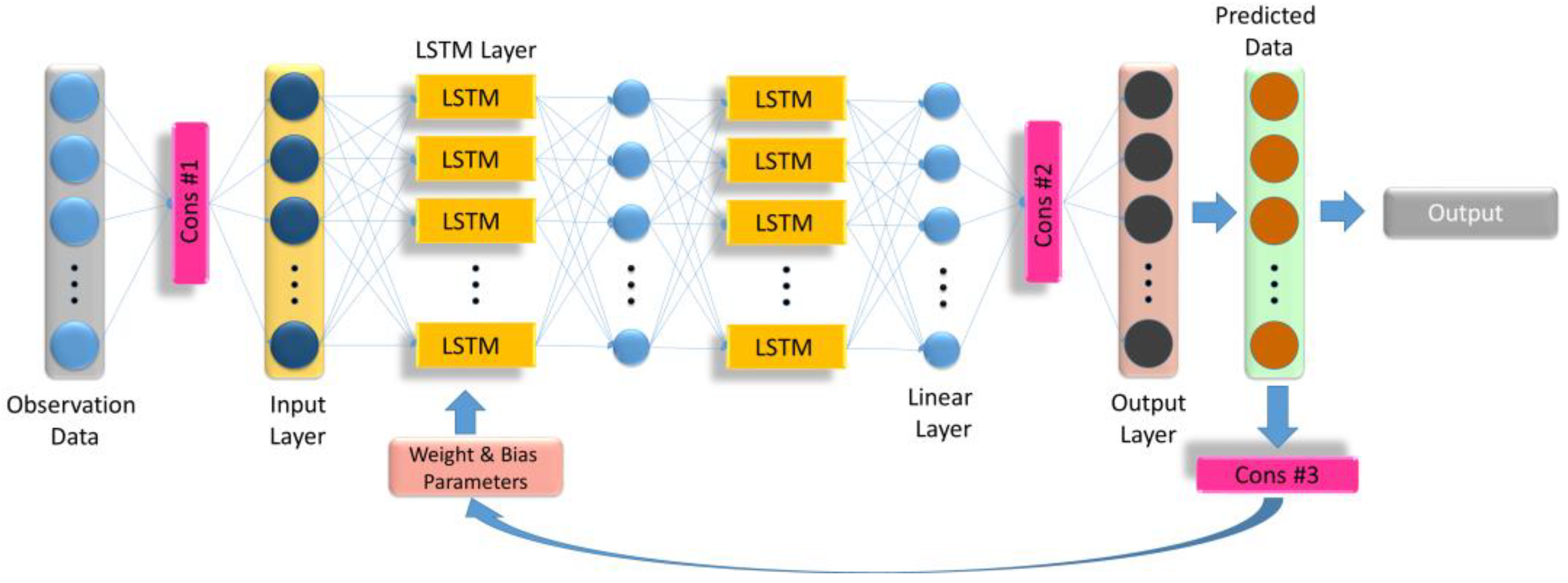
The PC-LSTM is designed using domain knowledge, and PV physical principles address the problems of modern Machine Learning (ML) algorithms, which are used on large amounts of data without taking physical laws into account (Figure 4). In creating the PC-LSTM, three types of restrictions (marked as Cons. #1, #2, #3) are used. The Data Filtering Module (DFM) is the initial module, and it divides the incoming data into distinct periods based on a flag variable. It filters training data to avoid physically improper forecasts, such as positive energy production at night, during training and testing. The PC-LSTM is based on global data or a basic concept of PV.
PV panels near the ground surface gather solar energy, which is crucial for power generation. As a result, it is critical to mark periods with positive SP on the ground. Using hourly Surface Energy (SE) values, the DFM does this automatically. During training, the model only uses data from the marked periods. In the prediction step, on the other hand, the resulting PV output will be computed correspondingly for periods when SE is predicted to be ‘0′. The efficiency of the PC-LSTM is increased to some extent by using fewer data points for model training. The Clipping Module (CM) is the second constraint included in the PC-LSTM; it is used to keep the model’s output within a tolerable range during training and testing. Using natural science to analyse PV avoids physical obstacles such as negative power generation. The model output should be positive because PV should be physically greater than ‘0′. As a result, the PC-LSTM output, y i , should satisfy the constraint in Equation (15).
y i ^ R e L U N N x i ; θ
A rectified linear unit function is ReLU(•). When ‘-ve’, the ReLU function returns ‘0′; when ‘+ve’, it returns the input value.
  • OWAWA-CNN-LSTM Forecasting Model
In this paper, the PC-LSTM and CNN-PM are applied. The generated value inside the OWAWA operator is the RMSE for such two models in different test cases (Figure 5). The formulation could remain unchanged from Equations (16)–(18):
P t wf   = OWAWA A W e PCLSTM , t , P PCLSTM , t , e CNN , t , P CNN , t = j = 1 2 w j P j , t
e PC - LSTM , t = P PC - LSTM , t P t P t
e CNN , t = P CNN , t P t P t
Pt is the measured WP at the time ‘t’, as megawatts (MW). P t wf   performs an OWAWA combined effectively with the WPF for point of time ‘t’. The WPF computed by the PCLSTM is P PC - LSTM , t , whereas the CNN model’s computation of WPF is P CNN , t . e PCLSTM , t and e CNN , t , are the flaws of these two PMs at point of time ‘t’. P j , t is the outcome of the WFM with the jth major error at point ‘t’. Solving the optimal control problem yields the weight values, w j . Min S W = t = 1 N P t P t w f 2 , Equation (19)
s . t .   j = 1 2 w j = 1 w j 0 , j = 1 , 2
As a principle for determining the weight constants, the size of squared errors (S/W) among Pt others P t w f is used.
The accuracy of other PMs, otherwise analysts, changes slightly the next day, as per [35]. The two models perform similarly when the weather is the same. The error dispersion of the two models differs when the current and predicted days have different weather classifications. As a result, the nearest day with the same weather type was selected instead of the previous day. The historical errors e PCLSTM , t and e CNN , t and values P PC - LSTM , t , P CNN   , t for an adjacent day are identified beneath each weather type.

3. Modelling MOACO-Based DRP

Residential, industrial, and commercial electricity customers are studied in this section, and the continuity equation demonstrates the modelling for their behaviour. Constraints show that each consumer’s total energy reduction per hour should be less than or equivalent to the highest number of its offerings, e.g., Equations (20)–(22)
R P r , t = R C r , t ζ r , t   , R C r , t R C t m a x
C P c , t = C C c , t ζ c , t   , C C c , t C C t m a x
I P i , t = I C i , t ζ i , t   , I C i , t I C t m a x
where the residential, profitable, and business consumers counts are ‘r’, ‘c’, and ‘i’; in period ‘t’, the proposal of energy load minimization by all consumers is R C r , t , in period ‘ t , C C c , t , and I C i , t are the load reduction proposed by all consumers. In time ‘ t , the proposal of maximum load minimization by all consumers is R C t max , C C t m a x , and I C t m a x ; the R P r , t ,   C P c , t , and I P i , t are denoted by ζ r , t , ζ c , t , and ζ i , t . For the proposed load reductions, the cost of load minimization for residential, marketable, and business users in period ‘t’ is reproduced.

3.1. Objective Functions

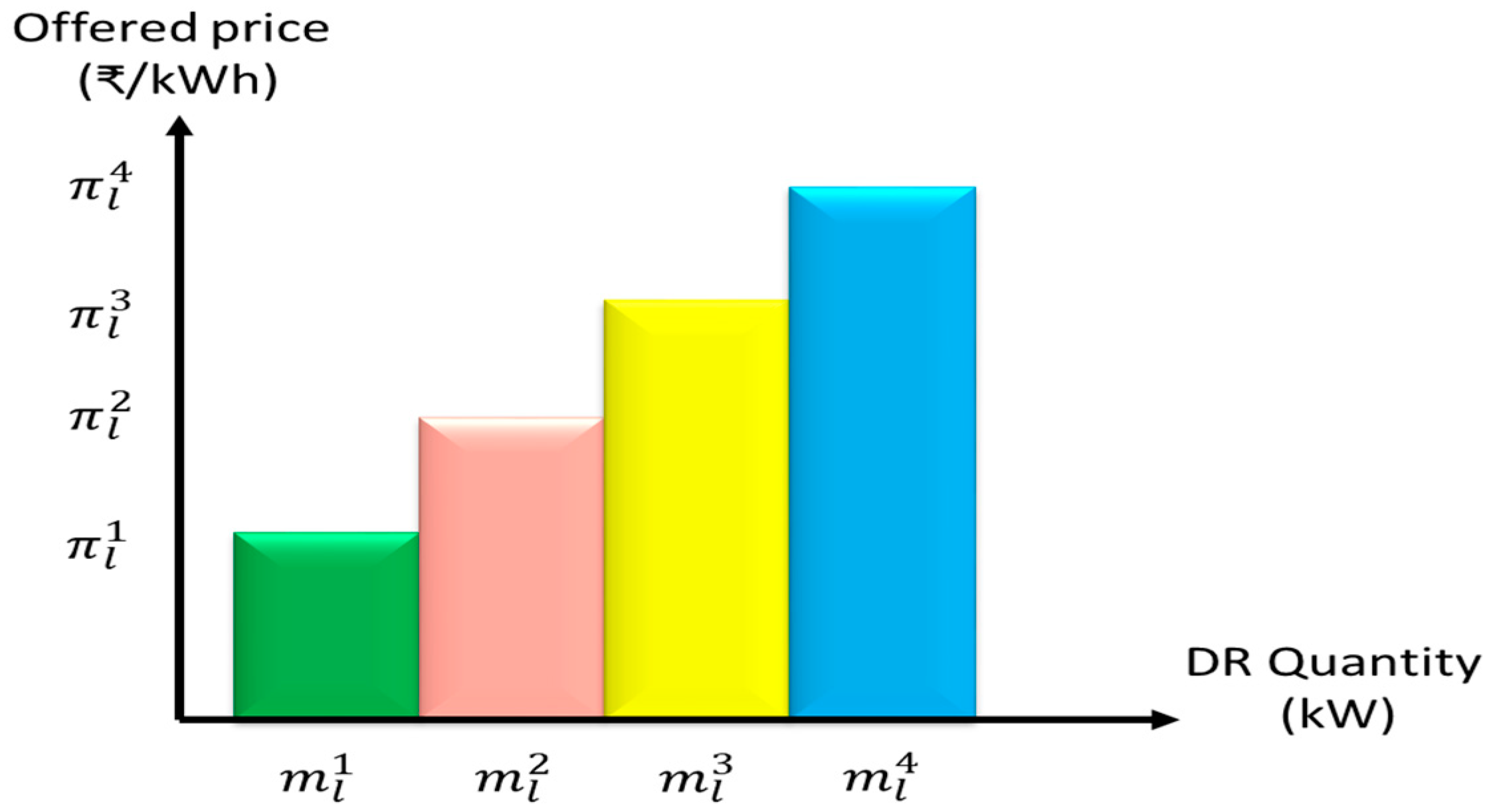
Price-and incentive-based DRP are the two types, with each group divided into subgroups depending on the consumer’s engagement in modifying their purchasing habits. Because incentive-based liability programmers deal with price signals and are therefore optional, assessing the DRP based upon incentive payments and modelling that on enabling retailers’ packages, given the lower quantity of requests, is shown in Figure 6.
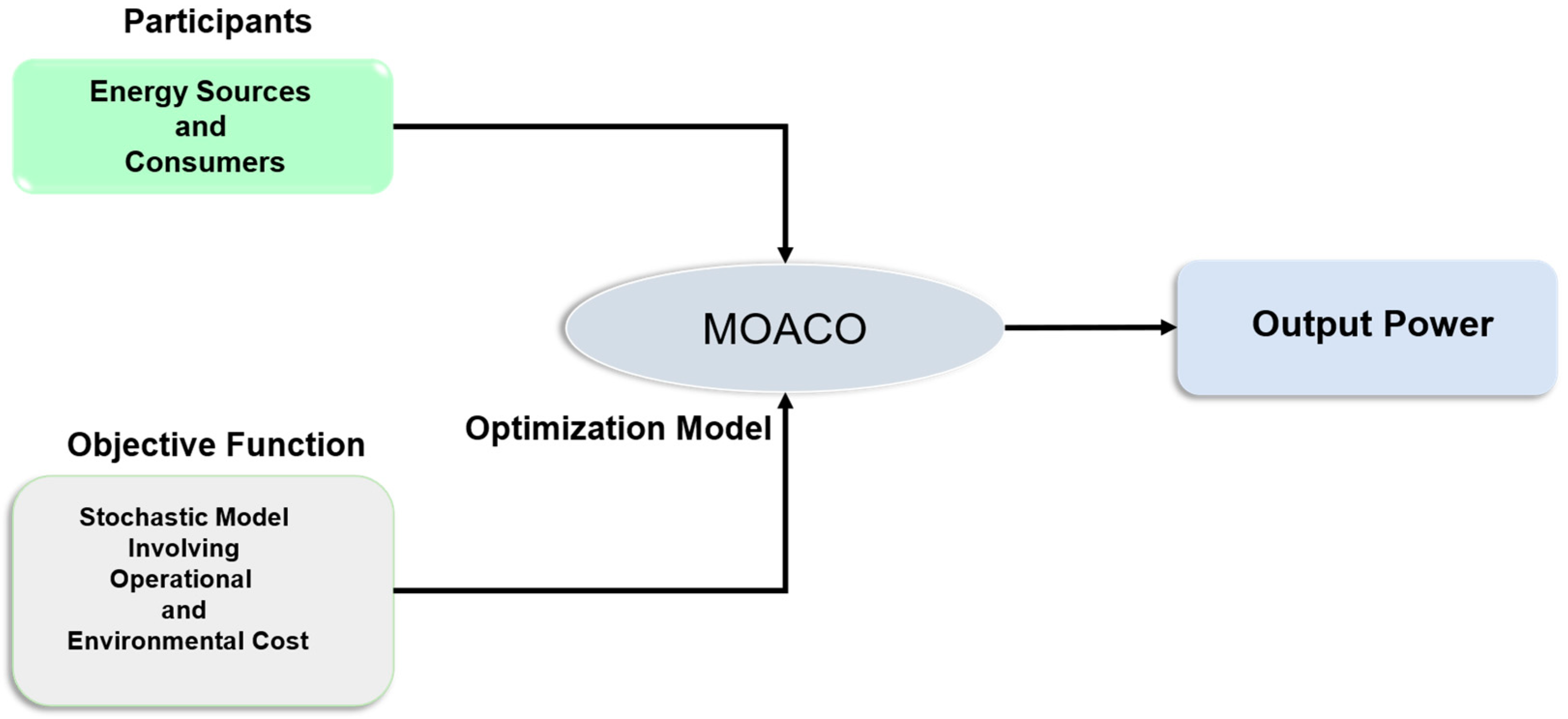
With scattered producing resources such as WP and SP, this study will use a Multi-Objective Stochastic Model (MOSM) to assess operation costs and emission levels. Furthermore, DRPs based on incentive-based payment will minimize the uncertainty caused by the unpredictability of WP and SP resource behaviour throughout a 24-h planning horizon. In these schemes, responding to demands is categorized as residential, industrial, or commercial. Figure 7 shows the proposed optimization model.

3.2. Operational Cost Function

Unpredicted operating costs are estimated by evaluating and understanding the chance for a scenario, Pr s , even in the ‘t’ period and the ‘s’ scenario that are prejudiced by the probabilistic. This component of an operational cost function comprises the cost of power savings due to DRP, and charges are linked to the Value of Lost Load (VOLL) and Expected Energy Not Served (EENS) to consumers.
M i n f 1 X = t = 1 T F C o s t t = t = 1 T C O C t + t = 1 T s = 1 S P r s × U O C s t  
wherein P r s is the possibility for scenario ‘s’. The operative costs, Equations (23) and (24), are confident and uncertain.
C O C t = i = 1 N D G P i t π i t I i t + S U i t I i t I i t 1 + R C i D G t + j = 1 J R C j D R t I B u y t P G r i d - B u y t π G r i d - B u y t I Sell   t P Grid - Sell   t π Grid - Sell   t U O C s t = i = 1 N D G C i , s D G t + j = 1 J C j , s D R t + E N S s t × V O L L t
where during the ‘t’ period, the output power and fixed cost for the ith unit’s amount are indicated by P i t and π i t ; during the tth period, the ON/OFF mode of the ith DG is represented by binary I i t ; during the tth period, the running and shut-off costs for the ith unit are represented by S U i t ; the ith DG and DRP for the jth load’s reserve costs are RC i DG and R C j D R ; in period ‘t’, the size of exchange power with utility is represented by P G r i d B u y t and P Grid - Sell t ; during the ‘t’ period, in the open electricity market the suggested cost for exchange power with utility is indicated by π G r i d - B u y t and π Grid - Sell   t ; during the tth period in the sth scenario, the ith DG unit’s running cost and the cost incurred for load minimization furnished by the jth DRPs are indicated by C i , s DG t and C j , s DR t . At the ‘t’ period and Value of Lost Load (VOLL) at the tth period, the Expected Energy Not Served (EENS) is E N S s t and   V O L L t . At each DG, the battery’s charge and discharge power and the switching of active power with the challenging grid produced by active power are included; X T = X 1 ,   X 2 ,   ,   X T is the variable’s state vector.
Regarding operational costs, DGs and DRP are reliable sources of reactive energy that make up for the lack of RE, SP, and WP. So, the DG is considered offline because its ground state is turned on to run standby power. As a result, the first part of the operating cost functions uses the fixed and start-up costs of DGs with a probability of one. In other words, when a situation in ON/OFF real-time mode happened, its DG stayed unchanged throughout the strategic planning process and power output was consumed only as per the day’s preset parameters. So, this reversing payment will not change in any real-time event of every scenario; therefore, the reserving cost is given a probability at the beginning of the objective function.

3.3. A Prototype of a Smart Grid System

The microgrid comprises DGs, energy reserves, and load systems that can run independently through the area’s main SG [36]. Its development remains a component of the SG notion; given the benefits of SG, such as lower energy costs and increased system dependability and safety, it is apparent that microgrids and SGs have common goals [37]. Furthermore, SG technologies are required for benefits such as green technology development and DRP microgrids. The SG analyses the following consumers: residential, business, marketable, and RES, such as Micro-Turbines (MT), Wind Turbines (WT), PV cells, Fuel Cells (FC), and battery and diesel generators. This SG transfers energy with the utility [38,39].

MOACO Algorithm

Equal inequalities and constraints should be solved concurrently in Multi-Objective Optimization Problems (MOOP) since there are many conflicting objective functions, Equation (25).
M i n   F X = [ f 1 X ,   f 2 X , , f n X ] T S u b j e c t   t o : g i X < 0                       i = 1 , 2 , , N u e q h i X = 0                       i = 1 , 2 , , N e q
where F(X) is an objective function and ‘X’ is an increment variable, fi(X) is the ‘i‘ objective function, gi(X) and hi(X) are equality and variation constraints, and ‘n’ is the number of objective functions. The possible solution for an MOOP is X or Y. The first solution will win, followed by the next, or none will control anything. As a result, if the two preceding conditions are met, one solution, ‘X’, will control the other in an optimization problem, Equation (26).
  j 1 , 2 , , n , f j X f j Y   k 1 , 2 , , n , f k X < f k Y
As a result, non-dominated search space results are used to find Pareto set solutions. Eventually, the solution is located among the non-dominated results in the collection (Algorithm 3).
Algorithm 3 MOACO
Input: Production volume, proposed energy price, DG operational and emission costs, the next day’s mean, and variance of WS and SP, and apply for demand from the daily load curve
Step 1: Obtaining the volume of WP and SP from the proposed statical model
Step 2: Set value parameters, number of ants (NA), and iterations (M)
Step 3: Generate a primary population as X T = X 1 ,   X 2 ,   ,   X T ;
Step 4: Calculate fitness function:
M i n f 1 X = t = 1 T F C o s t t = t = 1 T C O C t + t = 1 T s = 1 S P r s × U O C s t ;
Step 5: Initialize Pareto archive:= ;
Step 6: Identify and separate non-dominated results, and store them in the Pareto archive;
Step 7: Initialize all pheromone values to τ 0 ;
Step 8: While i < M Do:
Step 9: While j < N A Do:
Step 10: Identify new solution S using: j = arg max j S k i τ i , j ] α η i , j ] β   if   q q 0 J   otherwise     P k i , j = τ i , j ] α η i , j ] β w r k i τ i , u ] α η i , u ] β   if   j S k i 0   otherwise .  
Step 11: For each solution in the current ant population, measure the values of the corresponding objectives;
Step 12: Apply to update local rule using: τ i , j t = 1 ρ l τ i , j t 1 + ρ l τ 0 ;
Step 13: End Do;
Step 14: Update Pareto archive;
Step 15: While non-dominated solution Pareto archive Do:
Step 16: Apply to update global rule:   τ i , j t = 1 ρ g τ i , j t 1 + ρ g P S + C S S
Step 17: End Do;
Step 18: End Do;

4. NWP Simulation and Analysis

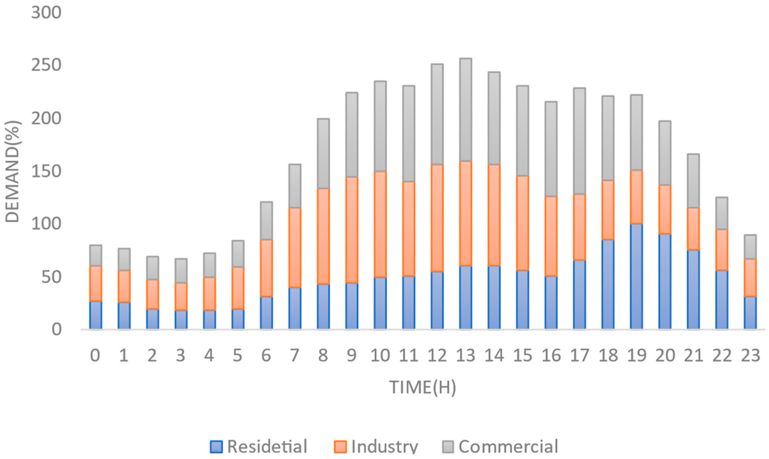
The SG taken into consideration is connected to the utility and includes three users: residential, industrial, and commercial, for which requirements and a daily load curve are provided (Figure 8). The prototype system has a total EC of 3246 kWh. The current market price for Indian Energy Exchange (IEX) is depicted in Figure 9. IEX initiated power trading in India and provided a digital platform for state electricity boards, power manufacturers, power traders, and open access consumers. The reserve cost of Conventional Energy (CE) sources is estimated to be 25% of the more profitable cost of energy generation. Hourly WS data are shown in Figure 10, sourced from the IMD Pune weather prediction website [40]. The solar cell in discussion seems to be a 30 kW Adani PV Module, made with P-type bifacial solar cells, characterised by 1000 and 200 W/m2 on the front and rear sides. Figure 11 depicts the average hourly SP sourced through the “Solar Energy Centre, Ministry of New and Renewable Energy, Government of India” [41].
With a power coefficient of 1, WT and PV systems adjust for reactive power locally by adding capacitors to related buses. The value of the lost load is estimated to be 1.54 V/kWh. A typical system with a 40 kWh battery charges from 10% to 100% of its capacity, with a 92% charge or discharge efficiency. Table 2 lists the DRP packages that are available. For DRP to be implemented, it is predictable that about 40% more consumers will enrol.
The problem is looked at differently to refer to how the energy level, reserve, and DR schedules affect operating costs and to clear up any confusion between WP and SP resources.
Case 1: Assuming the operational cost without DRP.
Case 2: Assuming the operational cost of DRP.
In all scenarios, power-producing units should be able to engage in the SG depending on their practical and commercial qualities, and in the presence of increased generation and demand, energy is exchanged only with the utility through a Point of Common Coupling (PCC). To verify the model’s effects, the proposed model was created using MATLAB R2022a software.
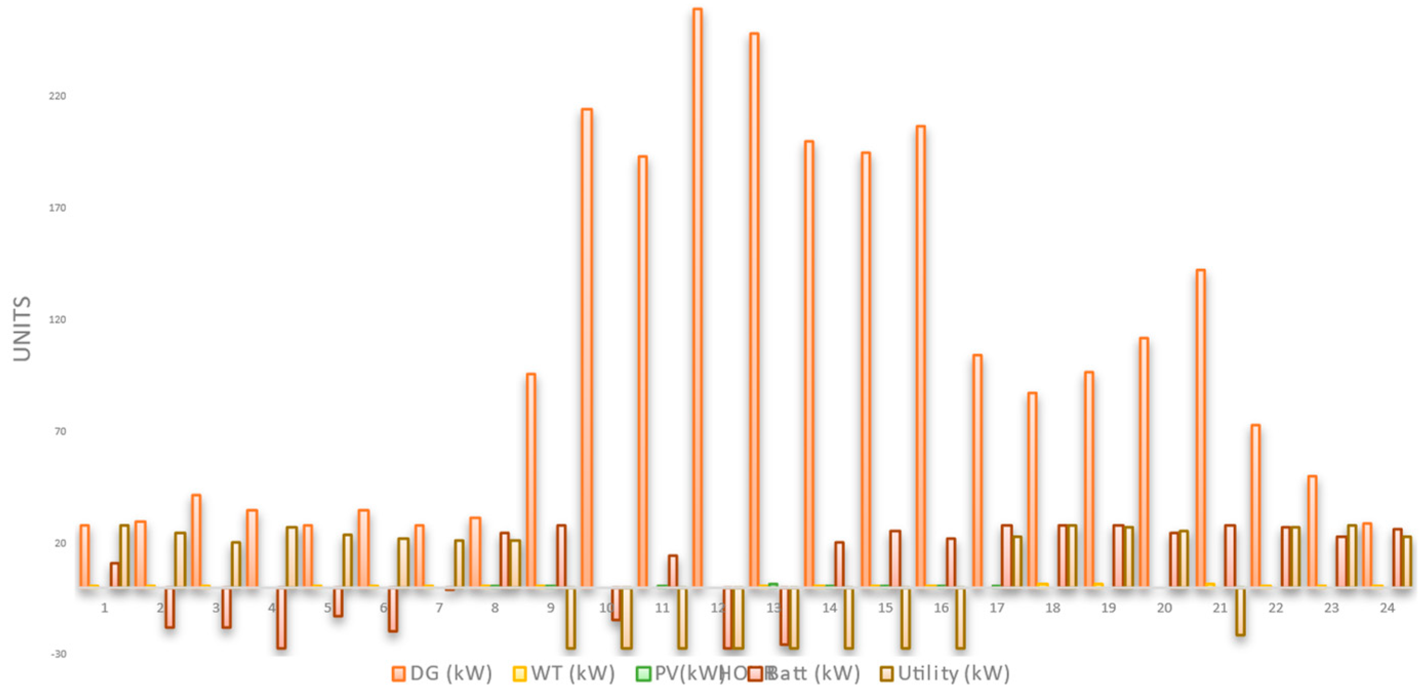
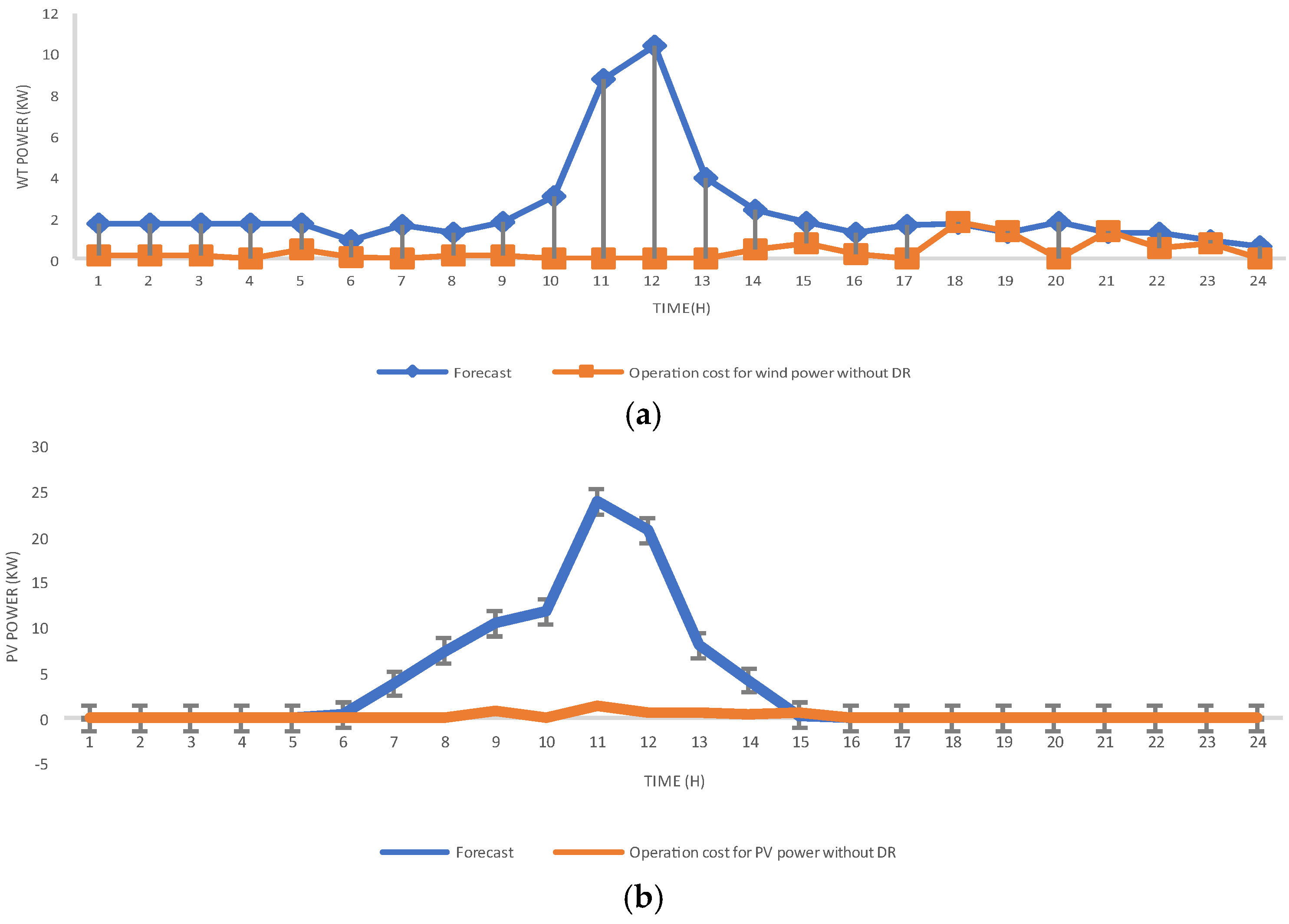
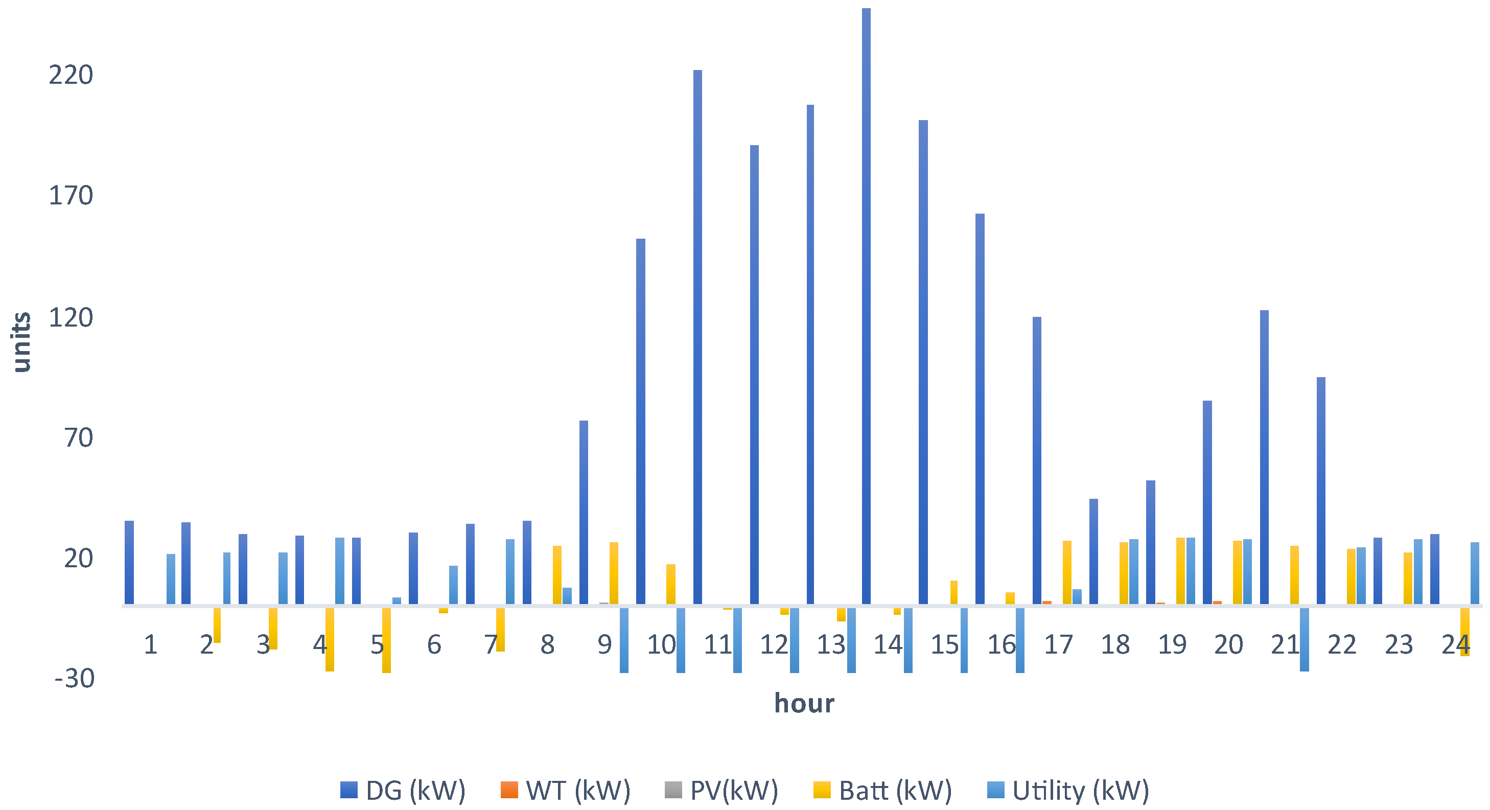
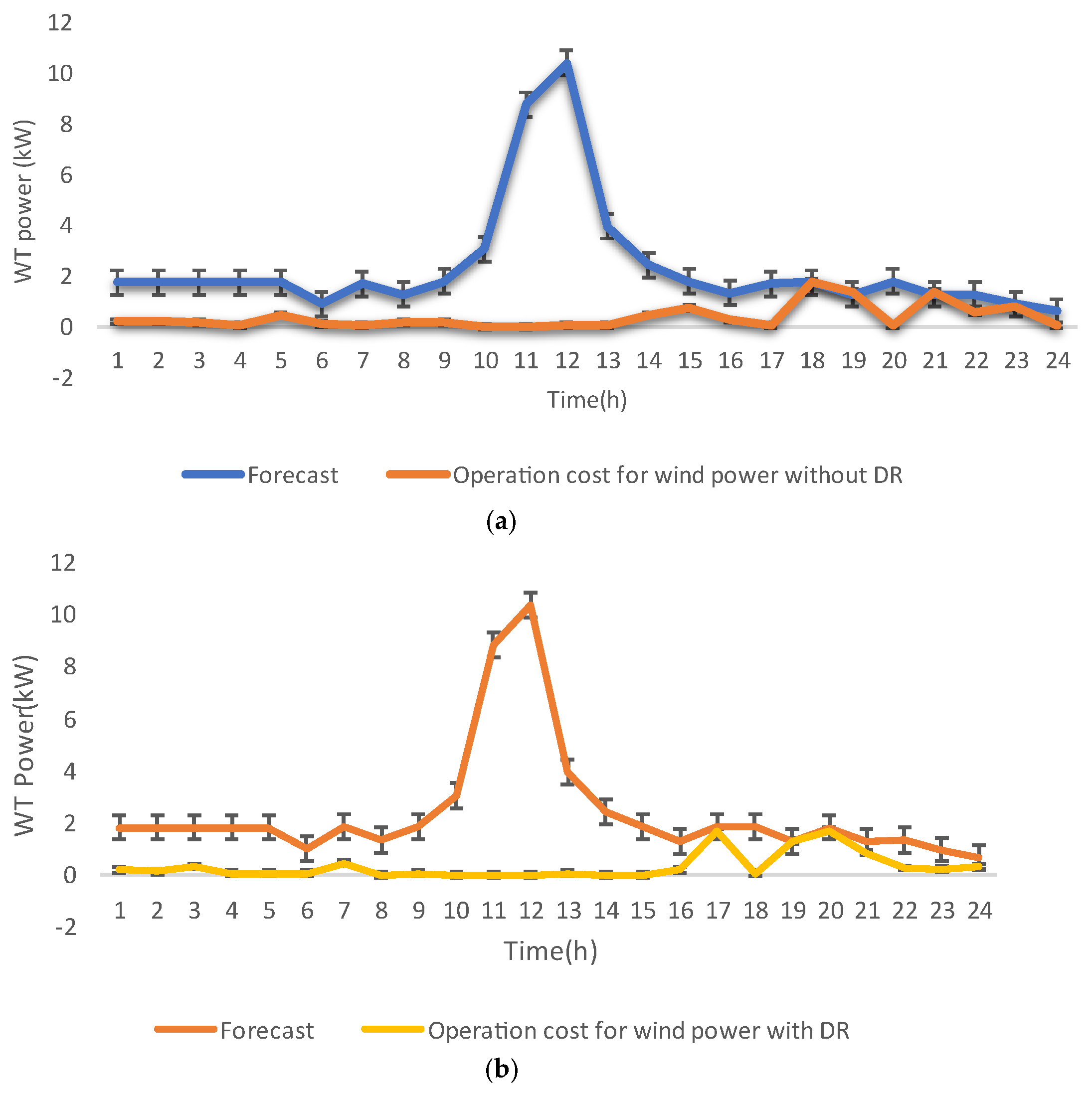
Case 1: Considering the cost of operations without the proposed DRP: From here, the operational costs are minimised independently without considering the DR. Figure 12 illustrates the best power generation allocation for lower operating costs. It shows that the battery begins to be charged early in the morning when energy costs are low, and whenever energy costs are high, the utility obtains energy from SG, wherein CEs prioritize power usage only at the lowest quoted price. The outcomes in Figure 13 show that the SG does not seek SP and WP. As a result, when evaluating the reasonable operational cost, they will not get much consideration.
Case 2: Costs and functionality of operations using DR: With the help of DR, operating costs are reduced independently. Figure 14 demonstrates the optimal power generation unit allocation for reducing operational costs. Although SP generation decreases from 4.54 to 3.15 kW, WP generation in the DRP decreases from 8.02 to 7.41 kW. These programs reduce SP and WP generation from 47.68 to 44.65 kW and 86.10 to 84.32 kW, respectively.
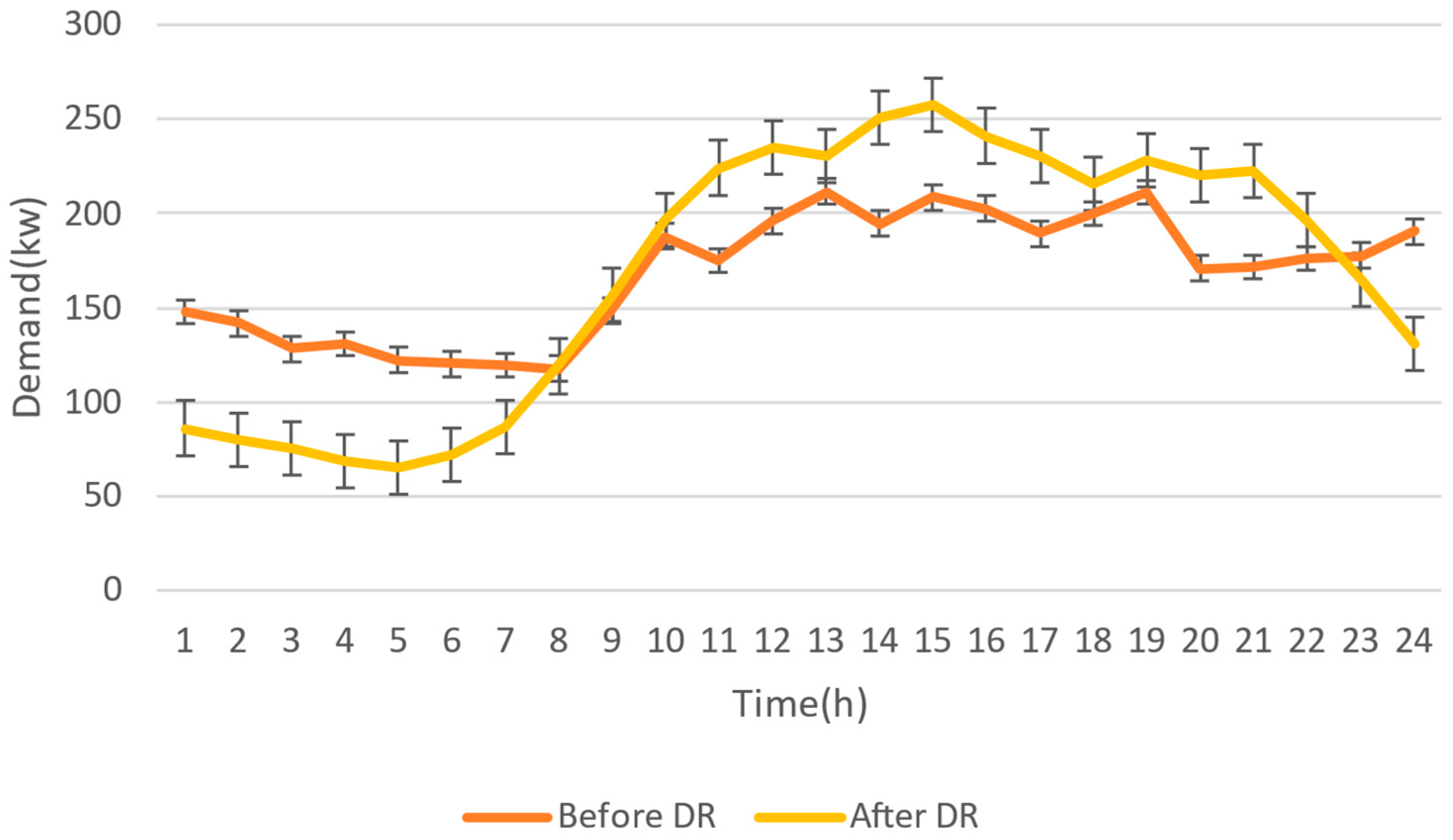
Figure 15 shows how much energy a WT and solar cell produce when operational costs and DR are considered. Figure 16 shows that using DRPs limits the amount of WT and solar cells that can be made while also shifting demand from peak to off-peak times. When consumers take part in the DRP and say they will use less power at a specific time, the system operator can lower the power of the generating units.
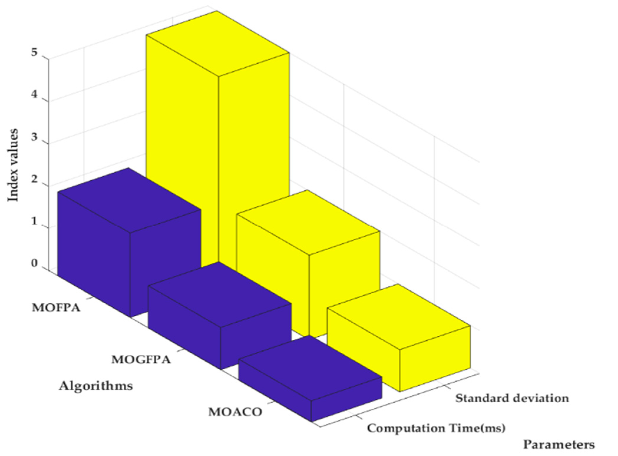
The performance evaluation of MOACO is shown through a comparison of standard deviation. Out of 50 runs, it has a minimal standard deviation of 1 unit. Additionally, the computational speed is faster, such as 0.5 ms.
To validate the results, two more algorithms in the literature have been taken to solve the problem as given in Table 3. We have implemented Multi-Objective Flower Pollination Algorithm (MOFPA) [23] and Multi-objective Golden Flower Pollination Algorithm (MOGFPA) [42] to validate the MOACO results. Comparatively, the standard deviation of MOACO is a lot less. At the same time, computation time is faster than the other two algorithms, as shown in the Figure 17.

5. Conclusions

The optimal demand-side management for the Smart Grid (SG) was implemented in this work by treating the Demand Response (DR) as the compensation for uncertainty produced by Wind Power (WP) and Solar Power (SP) generation in an optimization function with two conflicting goals. In numerous scenarios, the microgrid’s overall operational cost was assessed. Furthermore, Deep Learning (DL)-based Prediction Models (PM) for assessing WP and solar cell power generation were reported. The potential of energy exchange was envisaged for improved operation of the SG. Consumers are predicted to be engaged in DRPs based on incentive payments to manage consumption. To solve the given model and provide an optimal response, the MOACO method was applied. The simulations revealed that if customers employ DR and address production losses caused by uncertainty in WP and SP, it will reduce operating costs. In the future scope of research, this could be enriched with vehicle-to-grid techniques for optimal energy saving and management. Aggregator operations would also be considered for efficient operating conditions of the SG.

Author Contributions

Writing—review and editing, investigation, V.A.; validation, H.M.A.G.; Visualization, resources, Writing—review and editing D.A.P.; Supervision, I.V.P.; Project administration, V.S.P.; Software, Writing—review and editing M.A.; Writing—review and editing, P.K.; Conceptualization, methodology, writing—original draft preparation, S.S. All authors have read and agreed to the published version of the manuscript.

Funding

The authors also thank VIT management for supporting the APC for publication in this distinguished open access journal.

Institutional Review Board Statement

Not applicable.

Informed Consent Statement

Not applicable.

Data Availability Statement

Not applicable.

Conflicts of Interest

The authors declare no conflict of interest.

References

  1. Do Prado, J.; Qiao, W.; Qu, L.; Agüero, J. The Next-Generation Retail Electricity Market in the Context of Distributed Energy Resources: Vision and Integrating Framework. Energies 2019, 12, 491. [Google Scholar] [CrossRef]
  2. Johnson, J.; Quiroz, J.; Concepcion, R.; Wilches-Bernal, F.; Reno, M.J. Power System Effects and Mitigation Recommendations for DER Cyberattacks. IET Cyber-Phys. Syst. Theory Appl. 2019, 4, 240–249. [Google Scholar] [CrossRef]
  3. Strezoski, L.; Stefani, I. Utility DERMS for Active Management of Emerging Distribution Grids with High Penetration of Renewable DERs. Electronics 2021, 10, 2027. [Google Scholar] [CrossRef]
  4. Mina-Casaran, J.D.; Echeverry, D.F.; Lozano, C.A. Demand Response Integration in Microgrid Planning as a Strategy for Energy Transition in Power Systems. IET Renew. Power Gener. 2021, 15, 889–902. [Google Scholar] [CrossRef]
  5. Zhang, Y.; Huang, T.; Bompard, E.F. Big Data Analytics in Smart Grids: A Review. Energy Inform. 2018, 1, 8. [Google Scholar] [CrossRef]
  6. Regy, P.V.; Sarwal, R.; Stranger, C.; Fitzgerald, G.; Ningthoujam, J.; Gupta, A.; Singh, N. Turning around the Power Distribution Sector: Learnings and Best Practices from Reforms; NITI Aayog, RMI, and RMI India: New Delhi, India, 2021. [Google Scholar]
  7. Palaniappan, S.; Asokan, R.; Bharathwaj, S.; Sujaudeen, N. Automated Meter Reading System—A Study. Int. J. Comput. Appl. 2015, 116, 39–46. [Google Scholar] [CrossRef]
  8. Díaz Redondo, R.P.; Fernández-Vilas, A.; Fernández dos Reis, G. Security Aspects in Smart Meters: Analysis and Prevention. Sensors 2020, 20, 3977. [Google Scholar] [CrossRef]
  9. Khan, A.A.; Razzaq, S.; Khan, A.; Khursheed, F. Owais HEMSs and Enabled Demand Response in Electricity Market: An Overview. Renew. Sustain. Energy Rev. 2015, 42, 773–785. [Google Scholar] [CrossRef]
  10. Alavi, S.A.; Ahmadian, A.; Aliakbar-Golkar, M. Optimal Probabilistic Energy Management in a Typical Micro-Grid Based-on Robust Optimization and Point Estimate Method. Energy Convers. Manag. 2015, 95, 314–325. [Google Scholar] [CrossRef]
  11. Zakariazadeh, A.; Jadid, S.; Siano, P. Stochastic Multi-Objective Operational Planning of Smart Distribution Systems Considering Demand Response Programs. Electr. Power Syst. Res. 2014, 111, 156–168. [Google Scholar] [CrossRef]
  12. Zakariazadeh, A.; Jadid, S.; Siano, P. Economic-Environmental Energy and Reserve Scheduling of Smart Distribution Systems: A Multiobjective Mathematical Programming Approach. Energy Convers. Manag. 2014, 78, 151–164. [Google Scholar] [CrossRef]
  13. Rezaei, N.; Kalantar, M. Smart Microgrid Hierarchical Frequency Control Ancillary Service Provision Based on Virtual Inertia Concept: An Integrated Demand Response and Droop Controlled Distributed Generation Framework. Energy Convers. Manag. 2015, 92, 287–301. [Google Scholar] [CrossRef]
  14. Cicek, N.; Delic, H. Demand Response Management for Smart Grids With Wind Power. IEEE Trans Sustain. Energy 2015, 6, 625–634. [Google Scholar] [CrossRef]
  15. Afshar, K.; Shokri Gazafroudi, A. Application of Stochastic Programming to Determine Operating Reserves with Considering Wind and Load Uncertainties. J. Oper. Autom. Power Eng. 2007, 1, 96–109. [Google Scholar]
  16. Ininahazwe, H.; Muriithi, C.M.; Kamau, S. Optimal Demand-Side Management for Smart Micro Grid with Storage. J. Power Energy Eng. 2018, 6, 38–58. [Google Scholar] [CrossRef]
  17. Aghajani, G.R.; Shayanfar, H.A.; Shayeghi, H. Demand Side Management in a Smart Micro-Grid in the Presence of Renewable Generation and Demand Response. Energy 2017, 126, 622–637. [Google Scholar] [CrossRef]
  18. Trujillo, D.; Garcia Torres, E.M. Demand Response Due to the Penetration of Electric Vehicles in a Microgrid through Stochastic Optimization. IEEE Lat. Am. Trans. 2022, 20, 651–658. [Google Scholar] [CrossRef]
  19. Dehnavi, E.; Akmal, A.A.S.; Moeini-Aghtaie, M. Developing a Novel Zonal Congestion Management Based on Demand Response Programs Considering Dynamic Transmission Ratings. Int. J. Electr. Power Energy Syst. 2023, 146, 108779. [Google Scholar] [CrossRef]
  20. Farinis, G.Κ.; Kanellos, F.D. Integrated Energy Management System for Microgrids of Building Prosumers. Electr. Power Syst. Res. 2021, 198, 107357. [Google Scholar] [CrossRef]
  21. Erenoğlu, A.K.; Şengör, İ.; Erdinç, O.; Taşcıkaraoğlu, A.; Catalão, J.P.S. Optimal Energy Management System for Microgrids Considering Energy Storage, Demand Response and Renewable Power Generation. Int. J. Electr. Power Energy Syst. 2022, 136, 107714. [Google Scholar] [CrossRef]
  22. Zappa, W.; van den Broek, M. Analysing the Potential of Integrating Wind and Solar Power in Europe Using Spatial Optimisation under Various Scenarios. Renew. Sustain. Energy Rev. 2018, 94, 1192–1216. [Google Scholar] [CrossRef]
  23. De, M.; Das, G.; Mandal, K.K. An Effective Energy Flow Management in Grid-Connected Solar–Wind-Microgrid System Incorporating Economic and Environmental Generation Scheduling Using a Meta-Dynamic Approach-Based Multiobjective Flower Pollination Algorithm. Energy Rep. 2021, 7, 2711–2726. [Google Scholar] [CrossRef]
  24. Coddington, O.; Lean, J.L.; Pilewskie, P.; Snow, M.; Lindholm, D. A Solar Irradiance Climate Data Record. Bull. Amer. Meteor. Soc. 2016, 97, 1265–1282. [Google Scholar] [CrossRef]
  25. Blanc, P.; Espinar, B.; Geuder, N.; Gueymard, C.; Meyer, R.; Pitz-Paal, R.; Reinhardt, B.; Renné, D.; Sengupta, M.; Wald, L. Direct Normal Irradiance Related Definitions and Applications: The Circumsolar Issue. Sol. Energy 2014, 110, 561–577. [Google Scholar] [CrossRef]
  26. Chu, Y.; Pedro, H.T.C.; Coimbra, C.F.M. Hybrid Intra-Hour DNI Forecasts with Sky Image Processing Enhanced by Stochastic Learning. Sol. Energy 2013, 98, 592–603. [Google Scholar] [CrossRef]
  27. Florita, A.; Hodge, B.-M.; Orwig, K. Identifying Wind and Solar Ramping Events. In Proceedings of the 2013 IEEE Green Technologies Conference (GreenTech), Denver, Colorado, 4–5 April 2013; IEEE: Piscataway, NJ, USA, 2013; pp. 147–152. [Google Scholar]
  28. Chu, Y.; Urquhart, B.; Gohari, S.M.I.; Pedro, H.T.C.; Kleissl, J.; Coimbra, C.F.M. Short-Term Reforecasting of Power Output from a 48 MWe Solar PV Plant. Sol. Energy 2015, 112, 68–77. [Google Scholar] [CrossRef]
  29. Marquez, R.; Coimbra, C.F.M. Intra-Hour DNI Forecasting Based on Cloud Tracking Image Analysis. Sol. Energy 2013, 91, 327–336. [Google Scholar] [CrossRef]
  30. Du, P. Ensemble Machine Learning-Based Wind Forecasting to Combine NWP Output With Data From Weather Station. IEEE Trans Sustain. Energy 2019, 10, 2133–2141. [Google Scholar] [CrossRef]
  31. Jo, J.-M. Effectiveness of Normalization Pre-Processing of Big Data to the Machine Learning Performance. J. Korea Inst. Electron. Commun. Sci. 2019, 14, 547–552. [Google Scholar]
  32. Inman, R.H.; Pedro, H.T.C.; Coimbra, C.F.M. Solar Forecasting Methods for Renewable Energy Integration. Prog. Energy Combust. Sci. 2013, 39, 535–576. [Google Scholar] [CrossRef]
  33. Pedro, H.T.C.; Coimbra, C.F.M.; Lauret, P. Adaptive Image Features for Intra-Hour Solar Forecasts. J. Renew. Sustain. Energy 2019, 11, 036101. [Google Scholar] [CrossRef]
  34. Rethage, D.; Pons, J.; Serra, X. A Wavenet for Speech Denoising. In Proceedings of the 2018 IEEE International Conference on Acoustics, Speech and Signal Processing (ICASSP), Calgary, AB, Canada, 15–20 April 2018; IEEE: Piscataway, NJ, USA, 2018; pp. 5069–5073. [Google Scholar]
  35. Sze, V.; Chen, Y.-H.; Yang, T.-J.; Emer, J.S. Efficient Processing of Deep Neural Networks: A Tutorial and Survey. Proc. IEEE 2017, 105, 2295–2329. [Google Scholar] [CrossRef]
  36. Peng, H.; Long, F.; Ding, C. Feature Selection Based on Mutual Information Criteria of Max-Dependency, Max-Relevance, and Min-Redundancy. IEEE Trans. Pattern Anal. Mach. Intell. 2005, 27, 1226–1238. [Google Scholar] [CrossRef] [PubMed]
  37. Yager, R.R.; Filev, D.P. Induced Ordered Weighted Averaging Operators. IEEE Trans. Syst. Man Cybern. Part B (Cybernetics) 1999, 29, 141–150. [Google Scholar] [CrossRef]
  38. Mazzola, S.; Astolfi, M.; Macchi, E. A Detailed Model for the Optimal Management of a Multigood Microgrid. Appl. Energy 2015, 154, 862–873. [Google Scholar] [CrossRef]
  39. Kanchev, H.; Lu, D.; Colas, F.; Lazarov, V.; Francois, B. Energy Management and Operational Planning of a Microgrid with a PV-Based Active Generator for Smart Grid Applications. IEEE Trans. Ind. Electron. 2011, 58, 4583–4592. [Google Scholar] [CrossRef]
  40. The website belongs to Ministry of New and Renewable Energy (MNRE), Government of India. Available online: https://mnre.gov.in/ (accessed on 8 March 2023).
  41. Climate Research & Services. Data Supply Portal, Version 4.0. Available online: https://Dsp.Imdpune.Gov.In/ (accessed on 1 March 2019).
  42. Swaminathan, D.; Rajagopalan, A. Multi-Objective Golden Flower Optimization Algorithm for Sustainable Reconfiguration of Power Distribution Network with Decentralized Generation. Axioms 2023, 12, 70. [Google Scholar] [CrossRef]
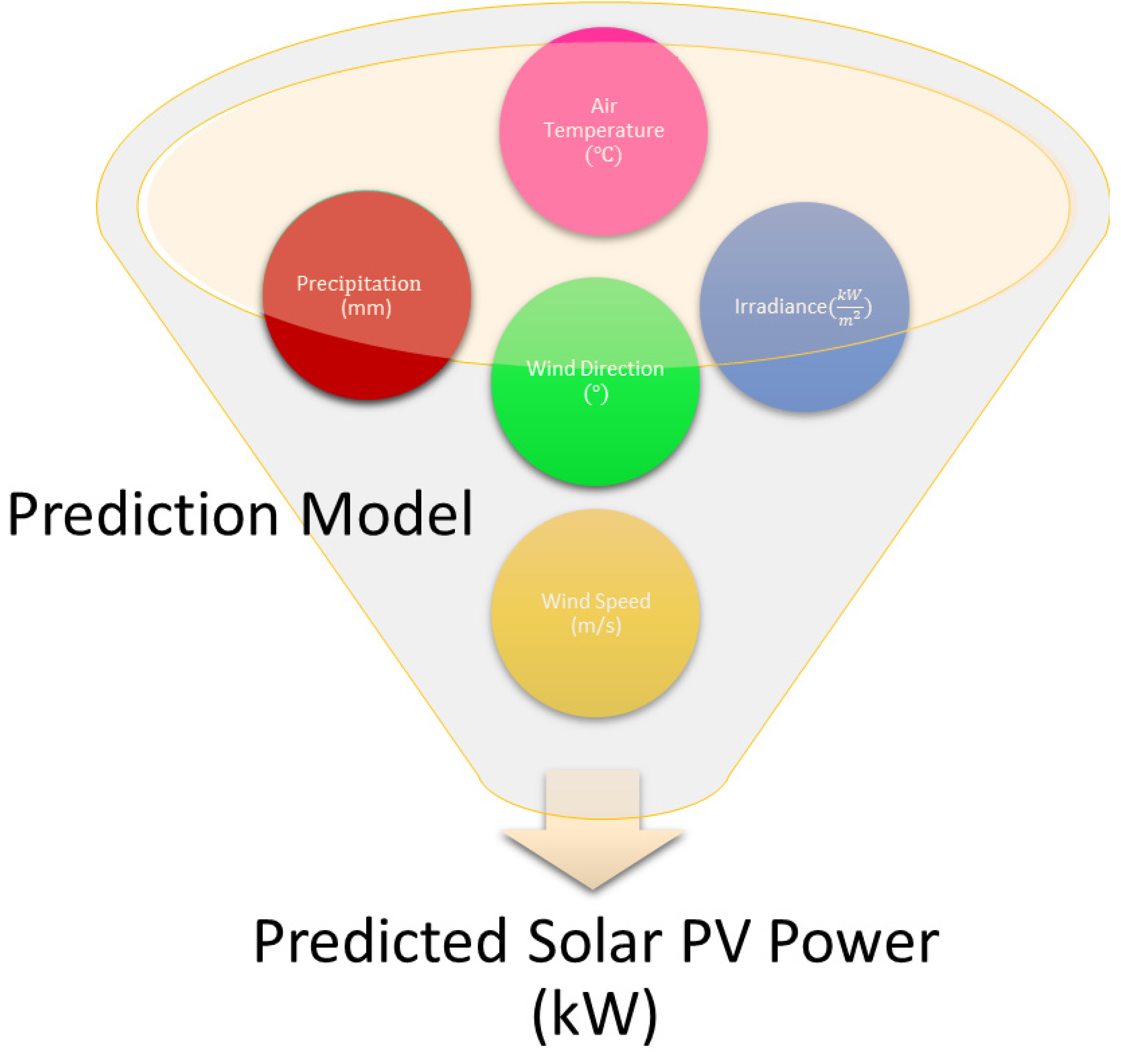
Figure 1. Solar PV-PM.
Sustainability 15 05453 g001
Figure 2. Illustration of an optimum day chosen on the left and a non-ideal day on the right (with a minor decrease at noon).
Sustainability 15 05453 g002
Figure 3. (a) VCNN and TCN-based Neural Network. (b) TCN Block Architecture. (c) ResBlock Architecture.
Sustainability 15 05453 g003
Figure 4. PC-LSTM architecture with three constraints.
Sustainability 15 05453 g004
Figure 5. The OWAWA-CNN-PCLSTM integrated WPF model.
Sustainability 15 05453 g005
Figure 6. The Package of DRP’s Offers.
Sustainability 15 05453 g006
Figure 7. The Optimization Model.
Sustainability 15 05453 g007
Figure 8. Daily load curves for different customers.
Sustainability 15 05453 g008
Figure 9. IEX market price in real-time (monthly chart).
Sustainability 15 05453 g009
Figure 10. Hourly WS forecast.
Sustainability 15 05453 g010
Figure 11. Hourly SP forecast.
Sustainability 15 05453 g011
Figure 12. Energy resource scheduling without DR.
Sustainability 15 05453 g012
Figure 13. Output power (a) WP; (b) PV power estimate without DR.
Sustainability 15 05453 g013
Figure 14. The operation cost of objective energy resource scheduling with DR.
Sustainability 15 05453 g014
Figure 15. Output power (a) Wind power estimate without DR; (b) Wind power estimate with DR; (c) PV power estimate with DR.
Sustainability 15 05453 g015aSustainability 15 05453 g015b
Figure 16. Pre- and post-DR load demand.
Sustainability 15 05453 g016
Figure 17. Comparative results of MOACO performance evaluation.
Sustainability 15 05453 g017
Table 1. Input variables for prediction applications.
ClassVariables
SPGHI, DNI, DIF, open-sky indices, spectrum energy, and neighbour energy.
Weather DataConditions such as pressure, temperature, humidity, Wind Speed (WS), wind direction, rainfall, aerosol optical depth, and cloud cover
Features of Sky ImagesCloud movement vector, cloud cover ratio, image features.
OtherSolar zenith, azimuth, local time, solar time
Table 2. Offered price package for DRP.
DRP-1kW0–1010–3030–6060–100
₹/kWh1.51.82.154.5
DRP-2kW0–1010–4040–6060–80
₹/kWh1.251.63.24.75
Table 3. Validation of MOACO with other algorithms.
AlgorithmsComputation Time (ms)Standard Deviation
MOFPA25
MOGFPA12
MOACO0.51
Disclaimer/Publisher’s Note: The statements, opinions and data contained in all publications are solely those of the individual author(s) and contributor(s) and not of MDPI and/or the editor(s). MDPI and/or the editor(s) disclaim responsibility for any injury to people or property resulting from any ideas, methods, instructions or products referred to in the content.