


Day-to-Day Dynamic Traffic Flow Assignment Model under Mixed Travel Modes Considering Customized Buses
Abstract
1. Introduction
2. Research Scope and Overview of Existing Studies
2.1. Smart Mobility
2.2. Day-to-Day Traffic Flow Assignment Model
2.3. Link Impedance Function
3. Characteristics of Different Travel Modes
3.1. Characteristics in Right-of-Way
3.2. Characteristics in Route Choice
3.3. Characteristics in Conversion of Travel Demand
4. Day-to-Day Dynamic Traffic Flow Assignment Model under Mixed Travel Modes Considering Customized Bus
- (1)
- Traffic flows considered in this paper include cars, conventional buses and customized buses.
- (2)
- Travelers have inertia in the travel mode selection, so the traffic flows of each travel mode remain stable in the evolution process.
- (3)
- Travelers consider travel time as travel costs in route selections, ignoring fuel and ticket costs.
- (4)
- Bus companies have enough conventional buses and customized buses to meet travelers’ travel demand.
4.1. Link Impedance Functions under Mixed Travel Modes
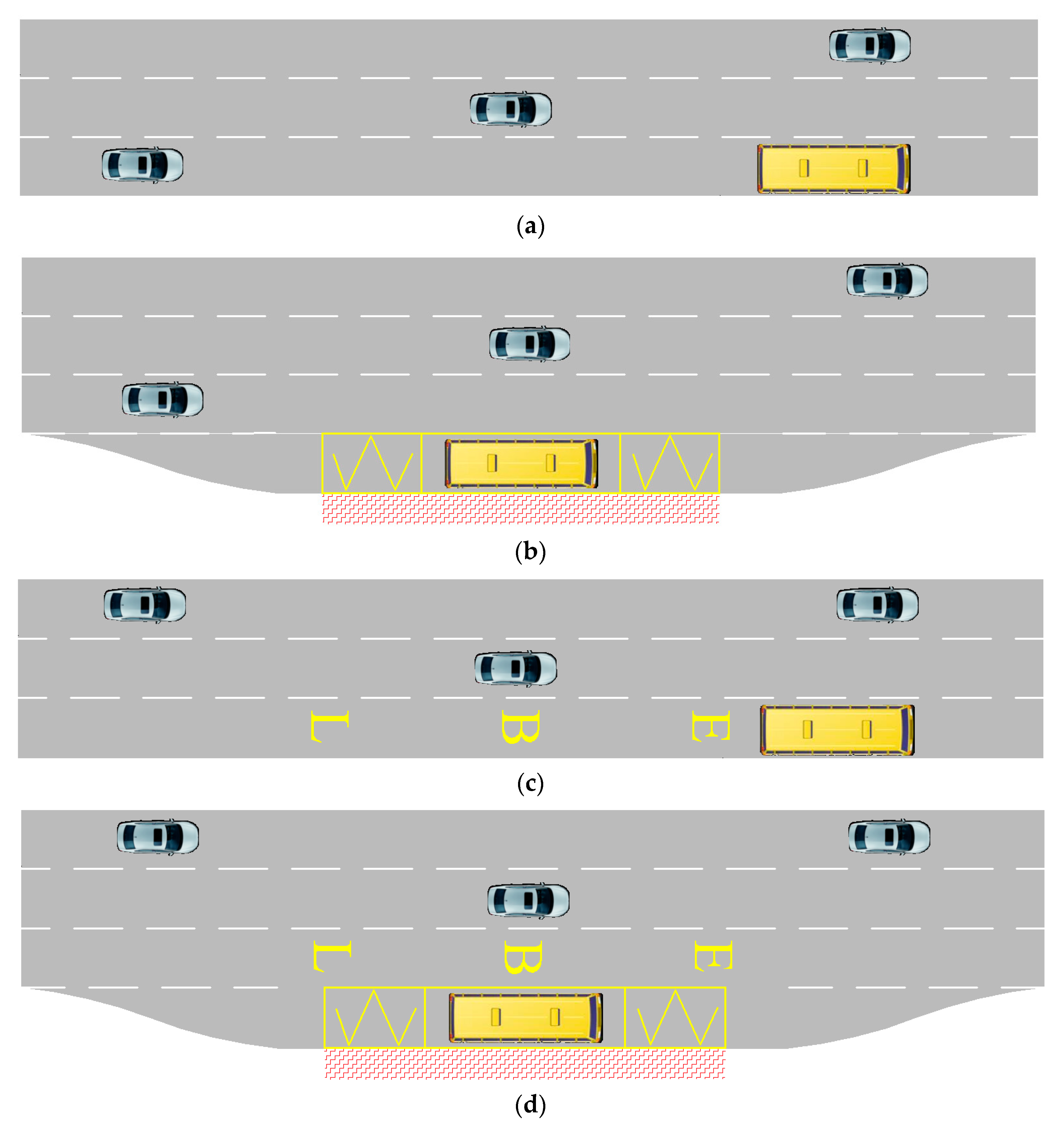
4.1.1. Classification of Links
4.1.2. Link Impedance Functions of the Car
4.1.3. Link Impedance Functions of the Conventional Bus
4.1.4. Link Impedance Functions of the Customized Bus
4.1.5. Correction of Actual Link Travel Time
4.2. Day-to-Day Traffic Flow Assignment Model Based on Routes
4.2.1. Statistics of Traffic Flows
4.2.2. Route Selection Model
4.2.3. Day-to-Day Updating Model of Travelers’ Perceived Travel Time
4.3. Algorithm for Solving the Model
5. Numerical Case Studies
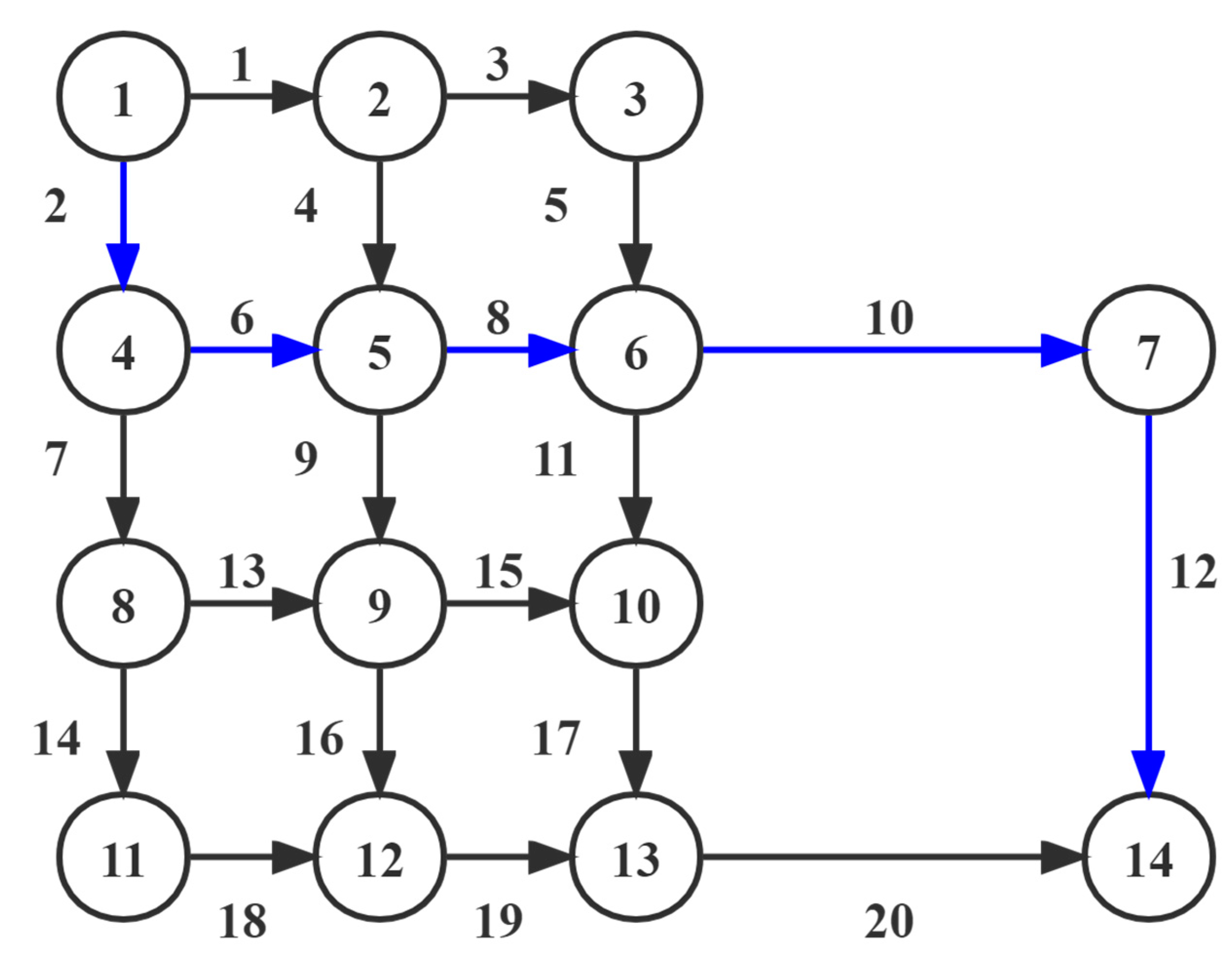
5.1. Network Introduction
5.2. Result Analysis
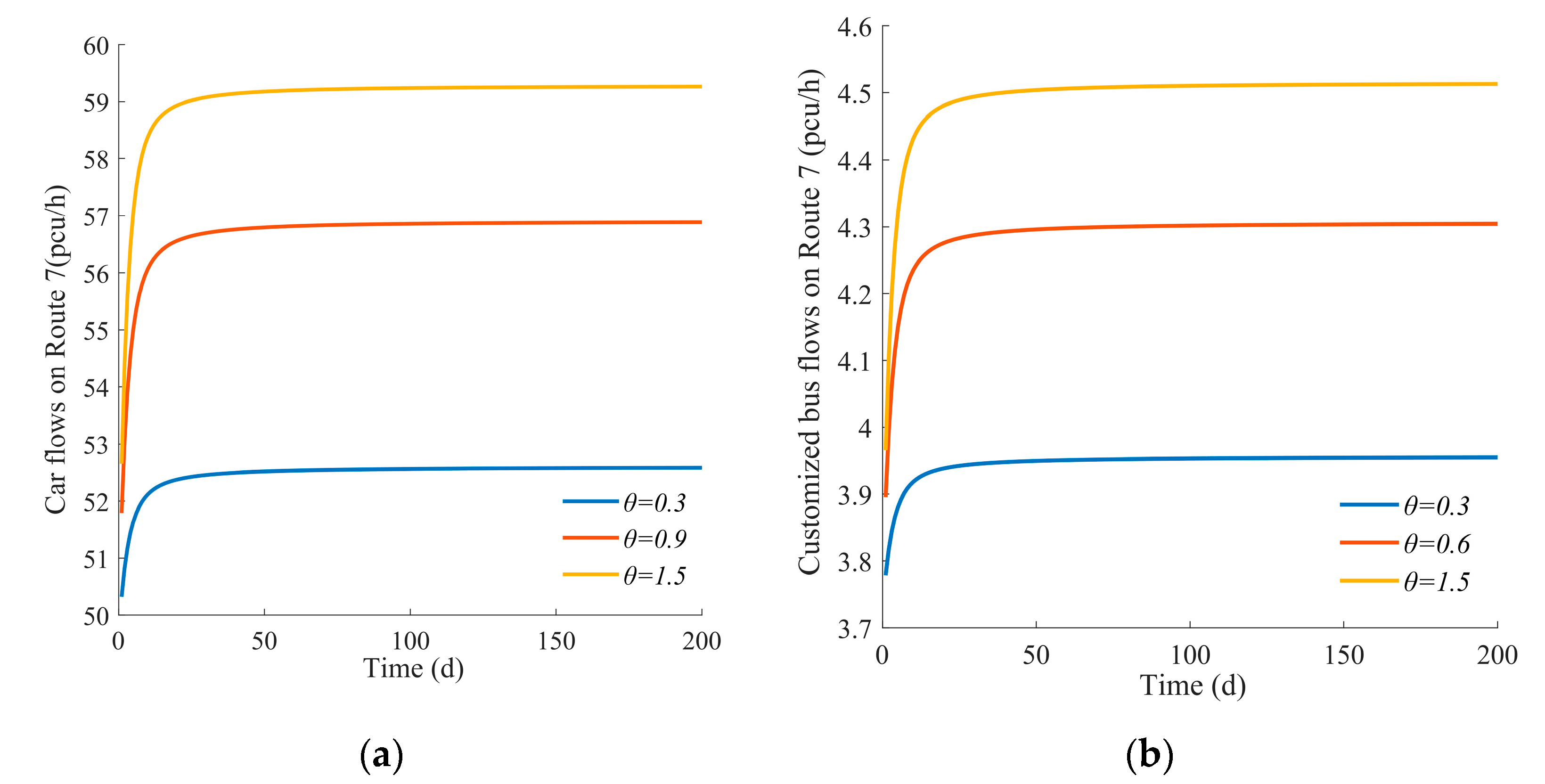
5.2.1. Study on the Influence of on Traffic Flow Evolution
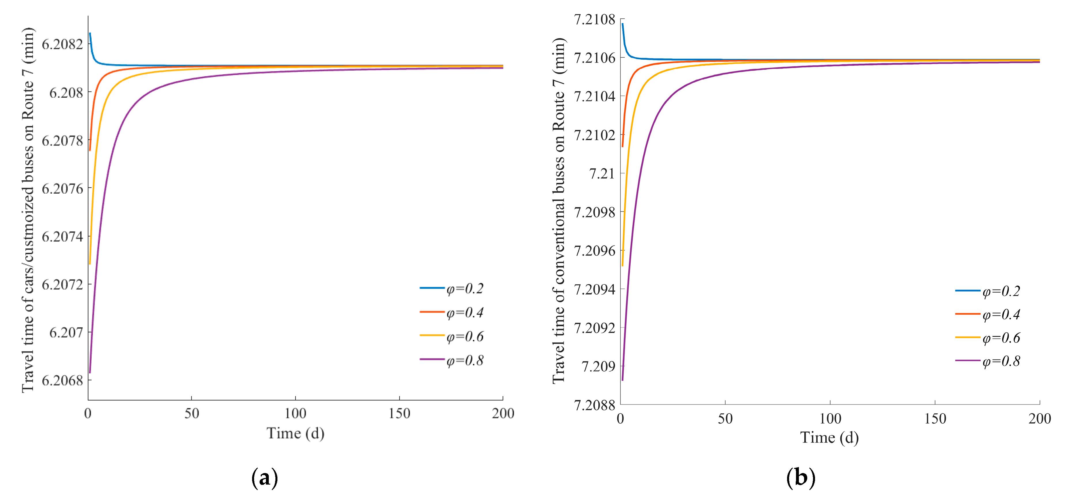
5.2.2. Study on the Influence of on Actual Travel Time
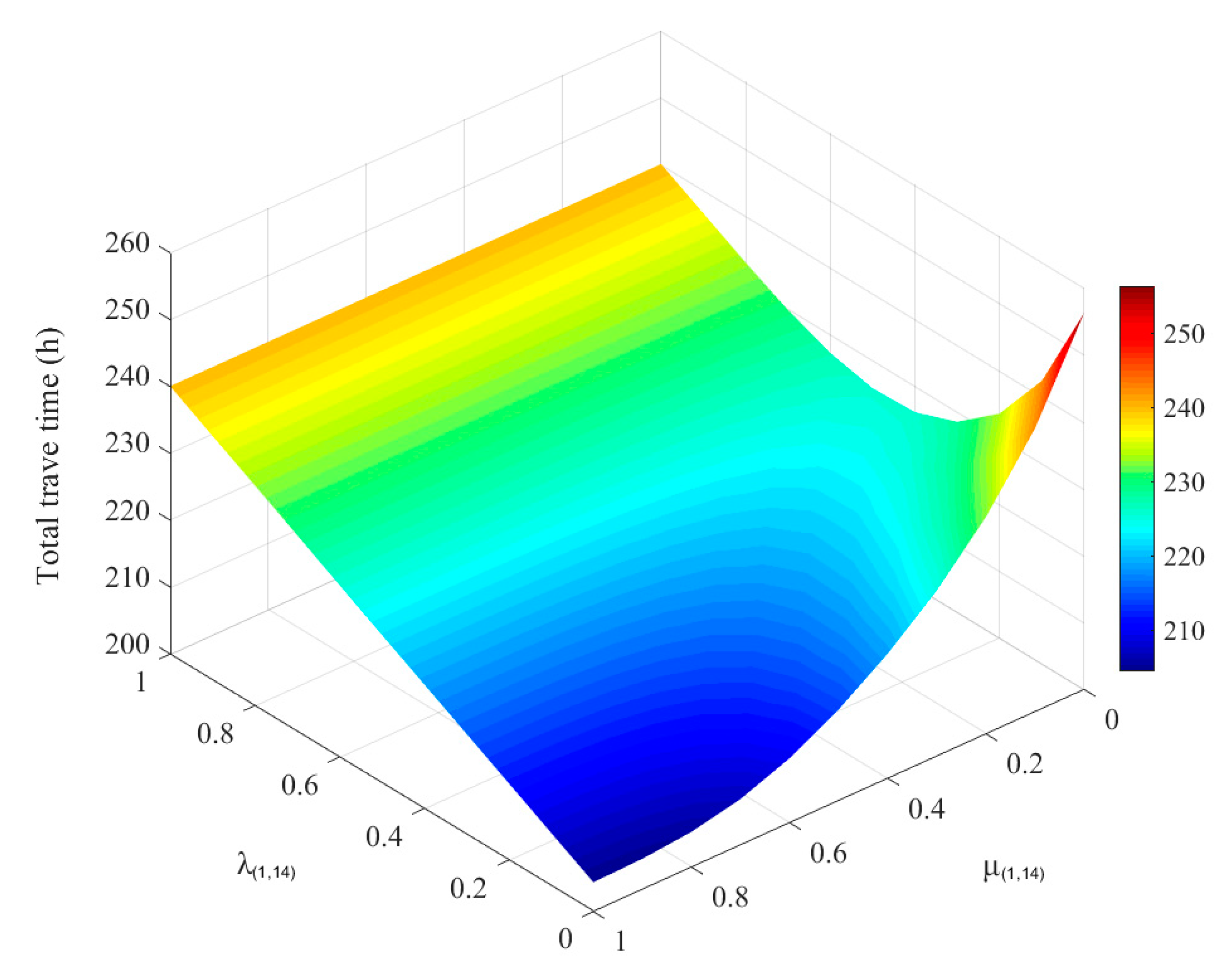
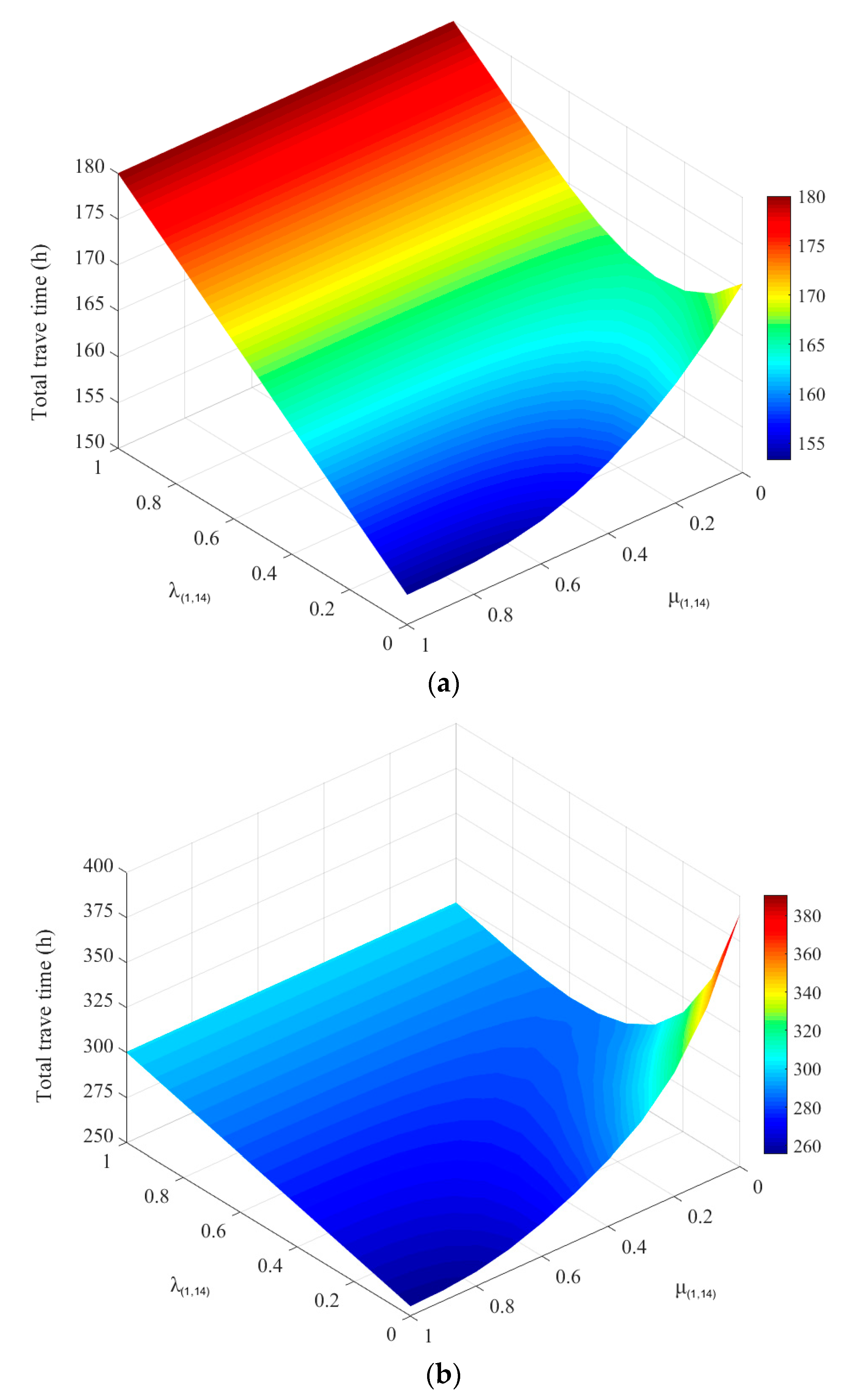
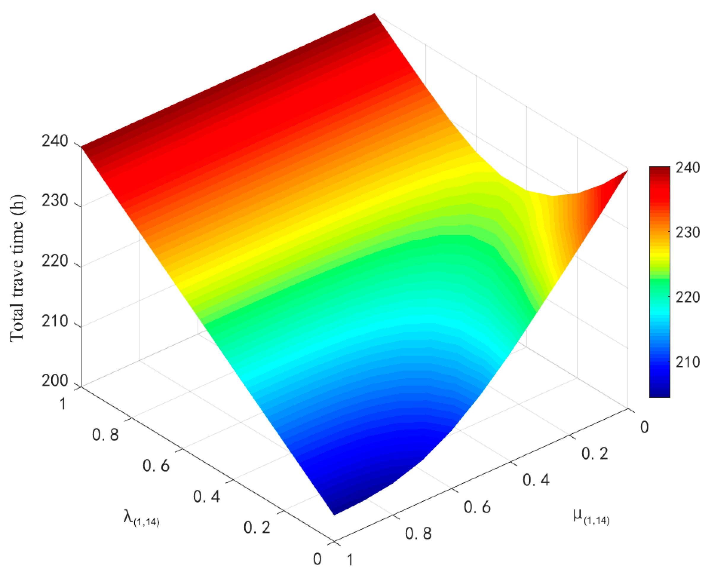
5.2.3. Study on the Influence of , and EBLs on the Total Travel Time of All Travelers
6. Conclusions and Suggestions
- (1)
- Whether the traffic network can finally reach an equilibrium state under mixed travel modes, and what kind of user equilibrium state it can reach, mainly depend on θ. When θ increases, the evolution speeds of network traffic flows increase, and the final state of the traffic network moves from SUE to DUE.
- (2)
- Trends of the actual travel time evolution of different travel modes are closely related to φ. The value of φ can not only influence the value of actual travel time, but also influence the evolution in direction of the actual travel time.
- (3)
- Conventional buses have higher transportation efficiency than cars, but if too many people choose conventional buses, the route conventional buses run on will become crowded, and the link resources in other links cannot be well utilized, which will make the total travel time increase in some circumstances. Customized buses not only have higher transportation efficiency than cars, but also can freely choose travel routes. The larger proportion of car travelers attracted by customized bus is always beneficial to reduce the total travel time.
- (4)
- When travel demands increase, the proportion of travelers who choose PT is required to increase to achieve the minimum total travel time.
- (5)
- Although the setting of EBLs can realize PT priority, the EBLs are not always beneficial, from the perspective of the whole traffic network in any case. When the traffic flows of conventional buses and customized buses are too light, EBLs have a negative effect on reducing the total travel time of all travelers in the traffic network. In fact, it is recommended to set EBLs when conventional buses and customized bus flows are heavy, which can be judged based on the model established in this paper.
- (1)
- The models in this paper assume that travelers have inertia in travel mode selection. The traffic flows of each travel mode remain stable in the evolution process. We only consider the traffic flow evolution caused by the route selection. In real life, some travelers may adjust their travel modes due to changes in the route travel time of different travel modes, which can be further considered.
- (2)
- As well as most studies, this paper considers travel time as well as travel cost. In fact, the travel cost in the broad sense may include many factors such as ticket price, oil price, comfort degree, and so on. These factors are considered by travelers when choosing travel modes and travel routes. Thus, various forms of travel cost should be considered in practical application.
Author Contributions
Funding
Institutional Review Board Statement
Informed Consent Statement
Data Availability Statement
Conflicts of Interest
References
- Zhao, F.; Zeng, X. Optimization of User and Operator Cost for Large-Scale Transit Network. J. Transp. Eng. 2007, 133, 240–251. [Google Scholar] [CrossRef]
- Liu, K.; Liu, J.; Zhang, J. Heuristic approach for the multiobjective optimization of the customized bus scheduling problem. IET Intell. Transp. Syst. 2022, 16, 277–291. [Google Scholar] [CrossRef]
- Yao, J.; Shi, F.; An, S.; Wang, J. Evaluation of exclusive bus lanes in a bi-modal degradable road network. Transp. Res. Part C Emerg. Technol. 2015, 60, 36–51. [Google Scholar] [CrossRef]
- Zheng, F.; Chen, J.; Wang, H.; Liu, H.; Liu, X. Developing a dynamic utilisation scheme for exclusive bus lanes on urban expressways: An enhanced CTM-based approach versus a microsimulation-based approach. IET Intell. Transp. Syst. 2020, 14, 1657–1664. [Google Scholar] [CrossRef]
- Yigitcanlar, T.; Han, H.; Kamruzzaman, M.; Ioppolo, G.; Sabatini-Marques, J. The making of smart cities. Land Use Policy 2019, 88, 104187. [Google Scholar] [CrossRef]
- Butler, L.; Yigitcanlar, T.; Paz, A. How Can Smart Mobility Innovations Alleviate Transportation Disadvantage? Assembling a Conceptual Framework through a Systematic Review. Appl. Sci. 2020, 10, 6306. [Google Scholar] [CrossRef]
- Flusberg, M. An Innovative Public Transportation System for a Small City: The Merrill, Wisconsin, Case Study. J. Transp. Res. Rec. 1976, 606, 54–59. Available online: https://trid.trb.org/view/52874 (accessed on 22 February 2023).
- Zhang, B.; Zhong, Z.; Zhou, X.; Qu, Y.; Li, F. Optimization Model and Solution Algorithm for Rural Customized Bus Route Operation under Multiple Constraints. Sustainability 2023, 15, 3883. [Google Scholar] [CrossRef]
- Han, S.; Fu, H.; Zhao, J.; Lin, J.; Zeng, W. Modelling and simulation of hierarchical scheduling of real-time responsive customised bus. IET Intell. Transp. Syst. 2020, 14, 1615–1625. [Google Scholar] [CrossRef]
- Montenegro, B.D.G.; Sörensen, K.; Vansteenwegen, P. A large neighborhood search algorithm to optimize a demand-responsive feeder service. Transp. Res. Part C Emerg. Technol. 2021, 127, 103102. [Google Scholar] [CrossRef]
- Antonio, P.; Marino, L.; Alessandro, F.; Chiara, P. Comparing Route Deviation Bus Operation with Respect to Dial-a-Ride Service for a Low-Demand Residential Area. In Proceedings of the Seventh International Conference on Data Analytics, DATA ANALYTICS, Athens, Greece, 18–22 November 2018; Available online: https://www.semanticscholar.org/paper/Comparing-Route-Deviation-Bus-Operation-with-to-for-Pratelli-Lupi/64aebff811a15fb28fe82b074ceb28582b098e33 (accessed on 22 February 2023).
- Alexandra, K.; Jan, G. From Public Mobility on Demand to Autonomous Public Mobility on Demand–Learning from Dial-A-Ride Services in Germany; Mobility in a Globalised World 2016; University of Bamberg Press: Bamberg, Germany, 2017; Available online: https://www.researchgate.net/publication/318982439_From_public_mobility_on_demand_to_autonomous_public_mobility_on_demand_-_Learning_from_dial-a-ride_services_in_Germany (accessed on 22 February 2023).
- An, J.Y.; Song, R.; Bi, M.K. Optimization flexible route design for high-speed railway station feeder bus. J. Transp. Syst. Eng. Inf. Technol. 2019, 19, 150. Available online: http://www.tseit.org.cn/EN/Y2019/V19/I5/150 (accessed on 22 February 2023).
- Wang, Z.; Luo, W.; Xu, S.; Yan, Y.; Huang, L.; Wang, J.; Hao, W.; Yang, Z. Electric Vehicle Lithium-Ion Battery Fault Diagnosis Based on Multi-Method Fusion of Big Data. Sustainability 2023, 15, 1120. [Google Scholar] [CrossRef]
- Xiong, R.; Yu, Q.; Shen, W.; Lin, C.; Sun, F. A Sensor Fault Diagnosis Method for a Lithium-Ion Battery Pack in Electric Vehicles. IEEE Trans. Power Electron. 2019, 34, 9709–9718. [Google Scholar] [CrossRef]
- Pan, F.W.; Gong, D.L.; Gao, Y.; Xu, W.M.; Ma, B. Current sensor fault diagnosis based on linearized model of lithium-ion battery. J. Jilin Univ. 2021, 51, 435–441. [Google Scholar] [CrossRef]
- Pan, F.W.; Ma, B.; Gao, Y.; Xu, M.; Gong, D. Parity space method for electric vehicle lithium-ion battery sensor fault diagnosis. Automot. Eng. 2019, 41, 831–838. [Google Scholar] [CrossRef]
- Schmid, M.; Gebauer, E.; Endisch, C. Structural Analysis in Reconfigurable Battery Systems for Active Fault Diagnosis. IEEE Trans. Power Electron. 2021, 36, 8672–8684. [Google Scholar] [CrossRef]
- Yang, N.; Xu, C.; Fang, R.; Li, H.; Xie, H. Capacity failure prediction of lithium batteries for vehicles based on large data. In Proceedings of the Second International Conference on Optoelectronic Science and Materials (ICOSM 2020), Hefei, China, 25–27 September 2020; Volume 11606, p. 1160609. [Google Scholar] [CrossRef]
- Zhao, X.; Wang, L.; Wang, X.; Sun, Y.; Jiang, T.; Li, Z.; Zhang, Y. Reliable Life Prediction and Evaluation Analysis of Lithium-ion Battery Based on Long-Short Term Memory Model. In Proceedings of the IEEE 19th International Conference on Software Quality, Reliability and Security Companion (QRS-C), Sofia, Bulgaria, 22–26 July 2019; pp. 507–510. [Google Scholar] [CrossRef]
- Zhao, J.; Ling, H.; Wang, J.; Burke, A.F.; Lian, Y. Data-driven prediction of battery failure for electric vehicles. iScience 2022, 25, 104172–104193. [Google Scholar] [CrossRef]
- Xue, Q.; Li, G.; Zhang, Y.; Shen, S.; Chen, Z.; Liu, Y. Fault diagnosis and abnormality detection of lithium-ion battery packs based on statistical distribution. J. Power Sources 2020, 482, 228964–228976. [Google Scholar] [CrossRef]
- Zhang, K.; Qu, D.; Song, H.; Wang, T.; Dai, S. Analysis of Lane-Changing Decision-Making Behavior and Molecular Interaction Potential Modeling for Connected and Automated Vehicles. Sustainability 2022, 14, 11049. [Google Scholar] [CrossRef]
- Qu, D.-Y.; Hei, K.-X.; Guo, H.-B. Game Behavior and Model of Lane-Changing on the Internet of Vehicles Environment. J. Jilin Univ. 2021, 1, 101–109. [Google Scholar] [CrossRef]
- Nilsson, J.; Silvlin, J.; Brannstrom, M.; Coelingh, E.; Fredriksson, J. If, When, and How to Perform Lane Change Maneuvers on Highways. IEEE Intell. Transp. Syst. Mag. 2016, 8, 68–78. [Google Scholar] [CrossRef]
- Guo, H.-B.; Qu, D.-Y.; Hong, J.-L. Vehicle Lane Changing Interaction Behavior and Decision Model Based on Utility Theory. Sci. Technol. Eng. 2020, 20, 12185–12190. [Google Scholar] [CrossRef]
- Moradi, M.; Assaf, G.J. Designing and Building an Intelligent Pavement Management System for Urban Road Networks. Sustainability 2023, 15, 1157. [Google Scholar] [CrossRef]
- Ma, L.; Li, Y.; Li, J.; Tan, W.; Yu, Y.; Chapman, M.A. Multi-Scale Point-Wise Convolutional Neural Networks for 3D Object Segmentation from LiDAR Point Clouds in Large-Scale Environments. IEEE Trans. Intell. Transp. Syst. 2019, 22, 821–836. [Google Scholar] [CrossRef]
- Tan, W.; Qin, N.; Ma, L.; Li, Y.; Du, J.; Cai, G.; Yang, K.; Li, J. Toronto-3D: A large-scale mobile LiDAR dataset for semantic segmentation of urban roadways. In Proceedings of the IEEE/CVF Conference on Computer Vision and Pattern Recognition Workshops, Seattle, WA, USA, 14–19 June 2020; pp. 202–203. [Google Scholar] [CrossRef]
- Shakhan, M.R.; Topal, A.; Sengoz, B. Data Collection for Implementation of the Mechanistic-Empirical Pavement Design Guide (MEPDG) in Izmir, Turkey. Tek. Dergi 2020, 36, 2021. [Google Scholar] [CrossRef]
- Tsai, Y.J.; Wu, Y.-C. Developing a Comprehensive Pavement Condition Evaluation System for Rigid Pavements in Georgia; Georgia Department of Transportation: Atlanta, GA, USA, 2019. Available online: https://rosap.ntl.bts.gov/view/dot/40264 (accessed on 22 February 2023).
- Singh, V.; Sahana, S.K.; Bhattacharjee, V. Nature-Inspired Cloud–Crowd Computing for Intelligent Transportation System. Sustainability 2022, 14, 16322. [Google Scholar] [CrossRef]
- Jovanovi’c, A.; Stevanovi’c, A.; Dobrota, N.; Teodorovi’c, D. Ecology based network traffic control: A bee colony optimization approach. Eng. Appl. Artif. Intell. 2022, 115, 105262. [Google Scholar] [CrossRef]
- Mohamed, S.A.E.; AlShalfan, K.A. Intelligent Traffic Management System Based on the Internet of Vehicles (IoV). J. Adv. Transp. 2021, 2021, 1–23. [Google Scholar] [CrossRef]
- Shi, Y.; Qi, Y.; Lv, L.; Liang, D. A Particle Swarm Optimisation with Linearly Decreasing Weight for Real-Time Traffic Signal Control. Machines 2021, 9, 280. [Google Scholar] [CrossRef]
- Mohamed, N.E.; Radwan, I.I. Traffic light control design approaches: A systematic literature review. Int. J. Electr. Comput. Eng. (IJECE) 2022, 12, 5355–5363. [Google Scholar] [CrossRef]
- Lin, H.; Han, Y.; Cai, W.; Jin, B. Traffic Signal Optimization Based on Fuzzy Control and Differential Evolution Algorithm. IEEE Trans. Intell. Transp. Syst. 2022, 23, 1–12. [Google Scholar] [CrossRef]
- Hosseinzadeh, M.; Sinopoli, B.; Kolmanovsky, I.; Baruah, S. MPC-Based Emergency Vehicle-Centered Multi-Intersection Traffic Control. IEEE Trans. Control. Syst. Technol. 2022, 31, 166–178. [Google Scholar] [CrossRef]
- Xiang, F.; Cheng, H.; Wang, Y. Exploring the Smart Street Management and Control Platform from the Perspective of Sustainability: A Study of Five Typical Chinese Cities. Sustainability 2023, 15, 3438. [Google Scholar] [CrossRef]
- Bagloee, S.A.; Sarvi, M.; Patriksson, M.; Rajabifard, A. A Mixed User-Equilibrium and System-Optimal Traffic Flow for Connected Vehicles Stated as a Complementarity Problem. Comput. Civ. Infrastruct. Eng. 2017, 32, 562–580. [Google Scholar] [CrossRef]
- Lou, X.-M.; Cheng, L.; Chu, Z.-M. Modelling travellers’ en-route path switching in a day-to-day dynamical system. Transp. B Transp. Dyn. 2017, 5, 15–37. [Google Scholar] [CrossRef]
- Zhou, B.; Xu, M.; Meng, Q.; Huang, Z. A day-to-day route flow evolution process towards the mixed equilibria. Transp. Res. Part C Emerg. Technol. 2017, 82, 210–228. [Google Scholar] [CrossRef]
- Yu, Y.; Han, K.; Ochieng, W. Day-to-day dynamic traffic assignment with imperfect information, bounded rationality and information sharing. Transp. Res. Part C Emerg. Technol. 2020, 114, 59–83. [Google Scholar] [CrossRef]
- Zhang, C.; Liu, T.-L.; Huang, H.-J.; Chen, J. A cumulative prospect theory approach to commuters’ day-to-day route-choice modeling with friends’ travel information. Transp. Res. Part C Emerg. Technol. 2018, 86, 527–548. [Google Scholar] [CrossRef]
- Huang, H.-J.; Liu, T.-L.; Yang, H. Modeling the evolutions of day-to-day route choice and year-to-year ATIS adoption with stochastic user equilibrium. J. Adv. Transp. 2008, 42, 111–127. [Google Scholar] [CrossRef]
- Li, K.; Wang, S.; Cong, R. Game dynamics of route choice in heterogenous population. Phys. Lett. A 2022, 421, 127775. [Google Scholar] [CrossRef]
- Sun, C.; Chu, Z.; Zhang, P.; Chang, Y.L. Day-to-day traffic user equilibrium model considering influence of intelligent highways and advanced traveler information systems. J. Cent. South Univ. 2022, 29, 1376–1388. [Google Scholar] [CrossRef]
- Fu, X.; Lam, W.H.; Chen, B.Y. A reliability-based traffic assignment model for multi-modal transport network under demand uncertainty. J. Adv. Transp. 2014, 48, 66–85. [Google Scholar] [CrossRef]
- Guo, R.-Y.; Huang, H.-J. Day-to-day dynamics in a duopoly ride-sourcing market. Transp. Res. Part C Emerg. Technol. 2022, 135, 103528. [Google Scholar] [CrossRef]
- Wu, J.; Ji, Y.; Sun, X.; Xu, Y. Guidance Optimization of Travelers’ Travel Mode Choice Based on Fuel Tax Rate and Bus Departure Quantity in Two-Mode Transportation System. J. Adv. Transp. 2020, 2020, 4190632. [Google Scholar] [CrossRef]
- Wang, Y.-Q.; Zhou, C.-F.; Jia, B.; Zhu, H.-B. Reliability analysis of degradable networks with modified BPR. Mod. Phys. Lett. B 2017, 31, 1750353. [Google Scholar] [CrossRef]
- US Bureau of Public Roads. Office of Planning. Urban Planning Division. In Traffic Assignment Manual for Application with a Large, High Speed Computer (Vol.2); US Department of Commerce: Washington, DC, USA, 1964; Available online: https://searchworks.stanford.edu/view/3216118 (accessed on 22 February 2023).
- Müller, S.; Schiller, C. Improvement of the volume-delay function by incorporating the impact of trucks on traffic flow. Transp. Plan. Technol. 2015, 38, 878–888. [Google Scholar] [CrossRef]
- Lu, Z.; Meng, Q.; Gomes, G. Estimating link travel time functions for heterogeneous traffic flows on freeways. J. Adv. Transp. 2016, 50, 1683–1698. [Google Scholar] [CrossRef]
- Thomas, J.; Srinivasan, K.K.; Arasan, V.T. Vehicle Class Wise Speed-Volume Models For Heterogeneous Traffic. Transport 2012, 27, 206–217. [Google Scholar] [CrossRef]
- Zhang, X.; Waller, S.T. Link performance functions for high occupancy vehicle lanes of freeways. Transport 2018, 33, 657–668. [Google Scholar] [CrossRef]
- Kim, D.; Schonfeld, P. Integrated Analysis of Toll Lanes and Bus Priority Lanes. Transp. Res. Rec. J. Transp. Res. Board 2008, 2076, 70–80. [Google Scholar] [CrossRef]
- Tranhuu, M.; Montgomery, F.; Timms, P. Modeling Bus Lane Priorities in a Motorcycle Environment Using SATURN. Transp. Res. Rec. J. Transp. Res. Board 2007, 2038, 167–174. [Google Scholar] [CrossRef]
- Mesbah, M.; Sarvi, M.; Currie, G.; Saffarzadeh, M. Policy-Making Tool for Optimization of Transit Priority Lanes in Urban Network. Transp. Res. Rec. J. Transp. Res. Board 2010, 2197, 54–62. [Google Scholar] [CrossRef]
- Sun, C.; Chang, Y.; Luan, X.; Tu, Q.; Tang, W. Origin-Destination Demand Reconstruction Using Observed Travel Time under Congested Network. Netw. Spat. Econ. 2020, 20, 733–755. [Google Scholar] [CrossRef]
- Wardrop, J.G. Some theoretical aspects of road traffic research. Proc. Inst. Civ. Eng. 1952, 1, 325–362. [Google Scholar] [CrossRef]
- Sun, C.; Zhang, P.; Shi, Y.; Chang, Y. Sensor Location Strategy and Scaling Rate Inference for Origin-Destination Demand Estimation. IEEE Trans. Intell. Transp. Syst. 2020, 22, 3455–3467. [Google Scholar] [CrossRef]
- Ministry of Housing and Urban-Rural Development of the People’s Republic of China. CJJ 37-90, Code for Design of Urban Road Engineering; China Architecture & Building Press, Beijing Municipal Engineering Research Institute: Beijing, China, 2006; Available online: https://max.book118.com/html/2016/0229/36381972.shtm (accessed on 22 February 2023).


| Type | EBL | Bus Stop |
|---|---|---|
| I | × | × |
| II | × | √ |
| III | √ | × |
| IV | √ | √ |
| Route No. | Relevant Links |
|---|---|
| 1 | 1→3→5→10→12 |
| 2 | 1→3→5→11→17→20 |
| 3 | 1→4→8→10→12 |
| 4 | 1→4→8→11→17→20 |
| 5 | 1→4→9→15→17→20 |
| 6 | 1→4→9→16→19→20 |
| 7 | 2→6→8→10→12 |
| 8 | 2→6→8→11→17→20 |
| 9 | 2→6→9→15→17→20 |
| 10 | 2→6→9→16→19→20 |
| 11 | 2→7→13→15→17→20 |
| 12 | 2→7→13→16→19→20 |
| 13 | 2→7→14→18→19→20 |
| Links No. | Type | Free-Flow Travel Time (min) | Capacity (pcu/min) | Capacity of the EBL (pcu/min) |
|---|---|---|---|---|
| 1 | I | 0.9 | 5 | 0 |
| 2 | II | 0.9 | 15 | 0 |
| 3 | I | 0.8 | 5 | 0 |
| 4 | I | 0.8 | 5 | 0 |
| 5 | I | 0.6 | 5 | 0 |
| 6 | III | 0.9 | 15 | 5 |
| 7 | I | 0.9 | 10 | 0 |
| 8 | IV | 0.9 | 20 | 10 |
| 9 | I | 0.9 | 5 | 0 |
| 10 | III | 1.7 | 30 | 15 |
| 11 | I | 0.9 | 5 | 0 |
| 12 | IV | 1.8 | 15 | 5 |
| 13 | I | 0.9 | 5 | 0 |
| 14 | 1 | 0.8 | 10 | 0 |
| 15 | I | 0.9 | 5 | 0 |
| 16 | I | 0.9 | 5 | 0 |
| 17 | I | 0.9 | 5 | 0 |
| 18 | I | 0.9 | 15 | 0 |
| 19 | I | 0.6 | 15 | 0 |
| 20 | I | 1.9 | 10 | 0 |
| θ | Car Flows on Route 7 within 200 Days | Customized Bus Flows on Route 7 within 200 Days | ||
|---|---|---|---|---|
| Mean (pcu/h) | Standard Deviation (pcu/h) | Mean (pcu/h) | Standard Deviation (pcu/h) | |
| 0.3 | 52.48 | 0.26 | 3.95 | 0.02 |
| 0.9 | 56.71 | 0.56 | 4.29 | 0.05 |
| 1.5 | 59.06 | 0.70 | 4.49 | 0.06 |
| λ(1,14) | 0 | 0.1 | 0.2 | 0.3 | 0.4 | 0.5 | 0.6 | 0.7 | 0.8 | 0.9 | 1 | |
|---|---|---|---|---|---|---|---|---|---|---|---|---|
| µ(1,14) | ||||||||||||
| 0 | 0 | 0 | 0 | 0 | 0 | 1 | 1 | 1 | 1 | 1 | 1 | |
| 0.1 | 0 | 0 | 0 | 0 | 1 | 1 | 1 | 1 | 1 | 1 | 1 | |
| 0.2 | 0 | 0 | 0 | 0 | 1 | 1 | 1 | 1 | 1 | 1 | 1 | |
| 0.3 | 0 | 0 | 0 | 1 | 1 | 1 | 1 | 1 | 1 | 1 | 1 | |
| 0.4 | 0 | 0 | 0 | 1 | 1 | 1 | 1 | 1 | 1 | 1 | 1 | |
| 0.5 | 0 | 0 | 1 | 1 | 1 | 1 | 1 | 1 | 1 | 1 | 1 | |
| 0.6 | 0 | 1 | 1 | 1 | 1 | 1 | 1 | 1 | 1 | 1 | 1 | |
| 0.7 | 1 | 1 | 1 | 1 | 1 | 1 | 1 | 1 | 1 | 1 | 1 | |
| 0.8 | 1 | 1 | 1 | 1 | 1 | 1 | 1 | 1 | 1 | 1 | 1 | |
| 0.9 | 1 | 1 | 1 | 1 | 1 | 1 | 1 | 1 | 1 | 1 | 1 | |
| 1 | 1 | 1 | 1 | 1 | 1 | 1 | 1 | 1 | 1 | 1 | 1 | |
Disclaimer/Publisher’s Note: The statements, opinions and data contained in all publications are solely those of the individual author(s) and contributor(s) and not of MDPI and/or the editor(s). MDPI and/or the editor(s) disclaim responsibility for any injury to people or property resulting from any ideas, methods, instructions or products referred to in the content. |
© 2023 by the authors. Licensee MDPI, Basel, Switzerland. This article is an open access article distributed under the terms and conditions of the Creative Commons Attribution (CC BY) license (https://creativecommons.org/licenses/by/4.0/).
Share and Cite
Chang, Y.; Wang, Y.; Sun, C.; Zhang, P.; Xu, W. Day-to-Day Dynamic Traffic Flow Assignment Model under Mixed Travel Modes Considering Customized Buses. Sustainability 2023, 15, 5440. https://doi.org/10.3390/su15065440
Chang Y, Wang Y, Sun C, Zhang P, Xu W. Day-to-Day Dynamic Traffic Flow Assignment Model under Mixed Travel Modes Considering Customized Buses. Sustainability. 2023; 15(6):5440. https://doi.org/10.3390/su15065440
Chicago/Turabian StyleChang, Yulin, Yijie Wang, Chao Sun, Peng Zhang, and Wenqian Xu. 2023. "Day-to-Day Dynamic Traffic Flow Assignment Model under Mixed Travel Modes Considering Customized Buses" Sustainability 15, no. 6: 5440. https://doi.org/10.3390/su15065440
APA StyleChang, Y., Wang, Y., Sun, C., Zhang, P., & Xu, W. (2023). Day-to-Day Dynamic Traffic Flow Assignment Model under Mixed Travel Modes Considering Customized Buses. Sustainability, 15(6), 5440. https://doi.org/10.3390/su15065440