
Modeling, Simulation, and Experimental Validation of a Novel MPPT for Hybrid Renewable Sources Integrated with UPQC: An Application of Jellyfish Search Optimizer


 ,
,  ,
,  , , and
Abstract
1. Introduction
- It presents an MPPT for a hybrid system of PV, wind, and FC during different operation circumstances.
- It utilizes conventional and intelligent optimization approaches for estimating MPPT.
- It employs UPQC for mitigating PQ problems.
- It experimentally validates the simulation results.
2. Hybrid Energy System
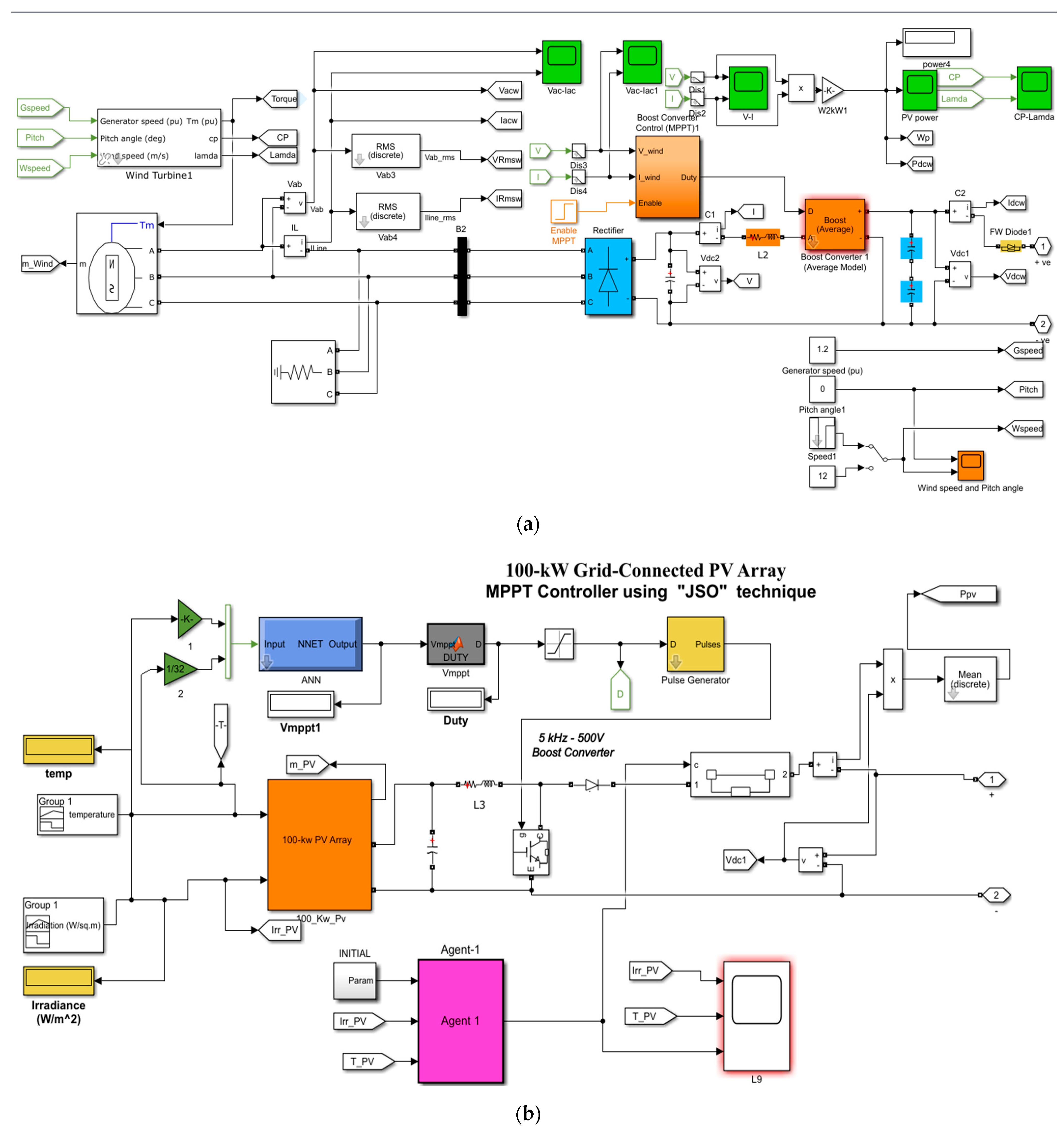
2.1. Modeling of PV System
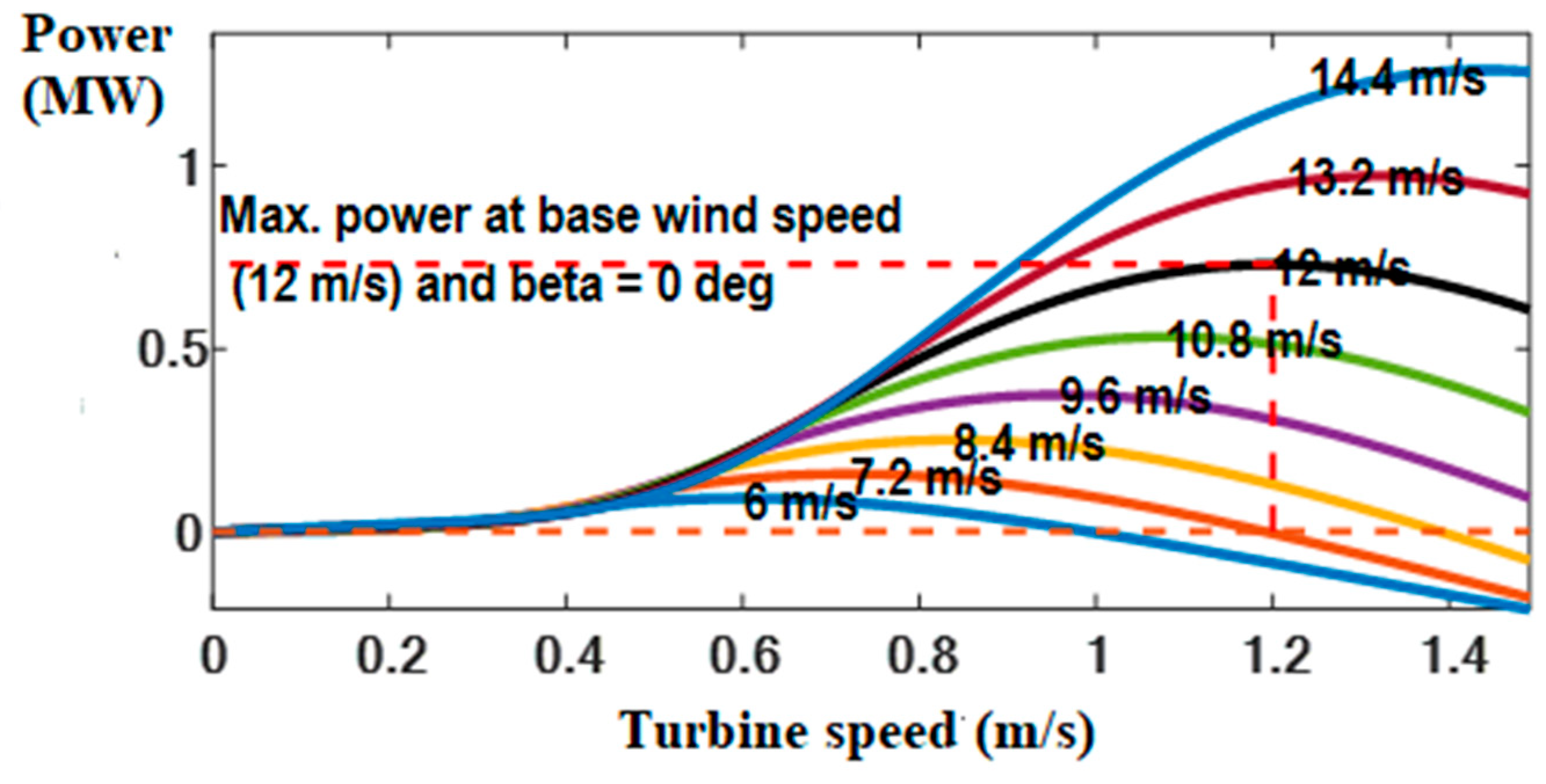
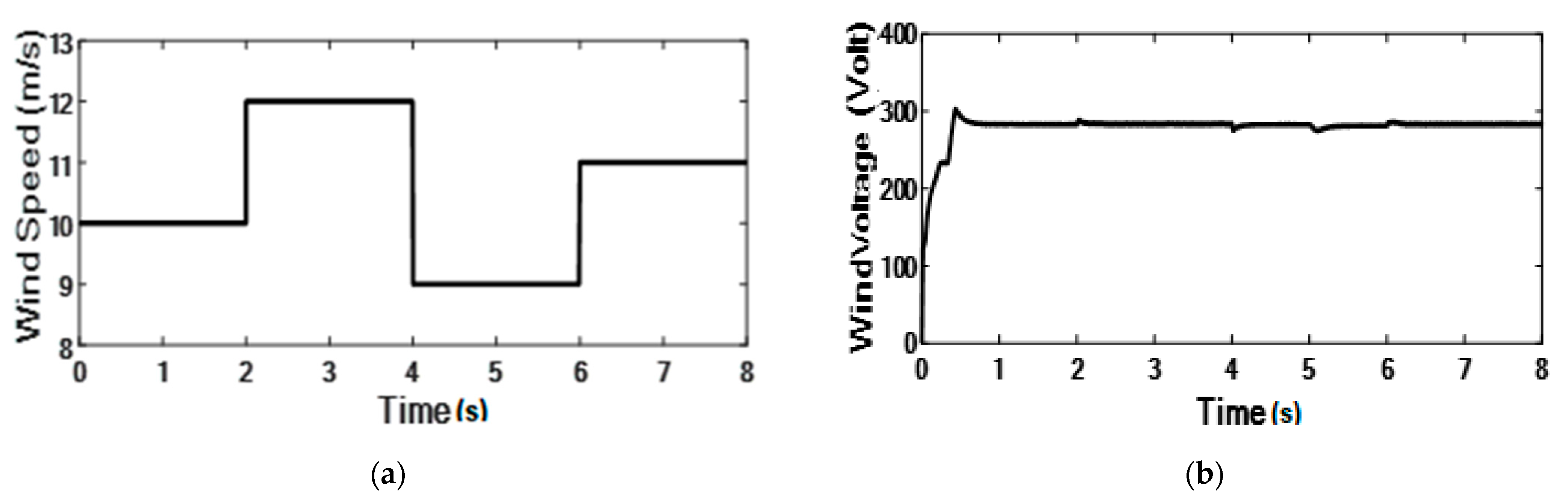
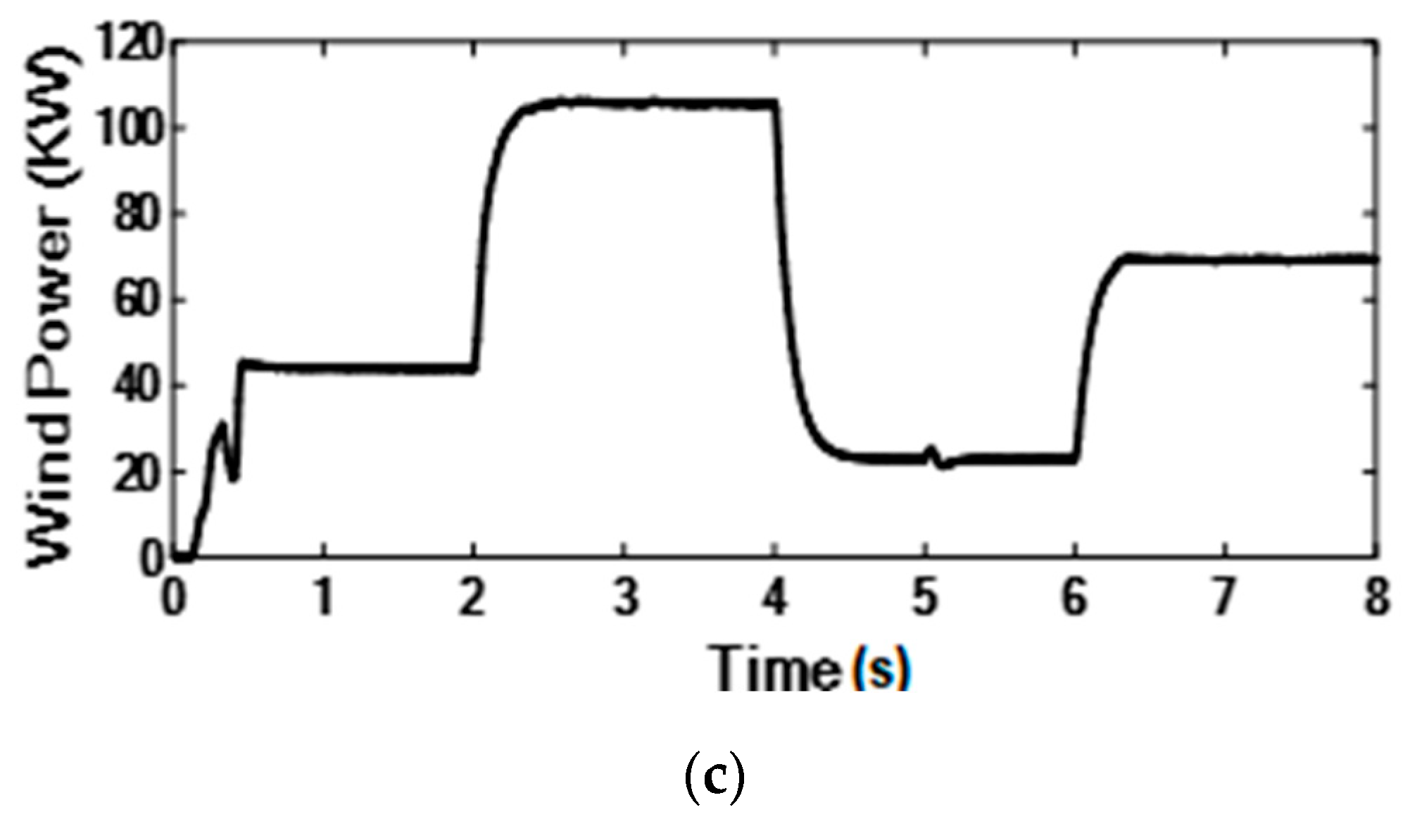
2.2. Modeling of the Wind System
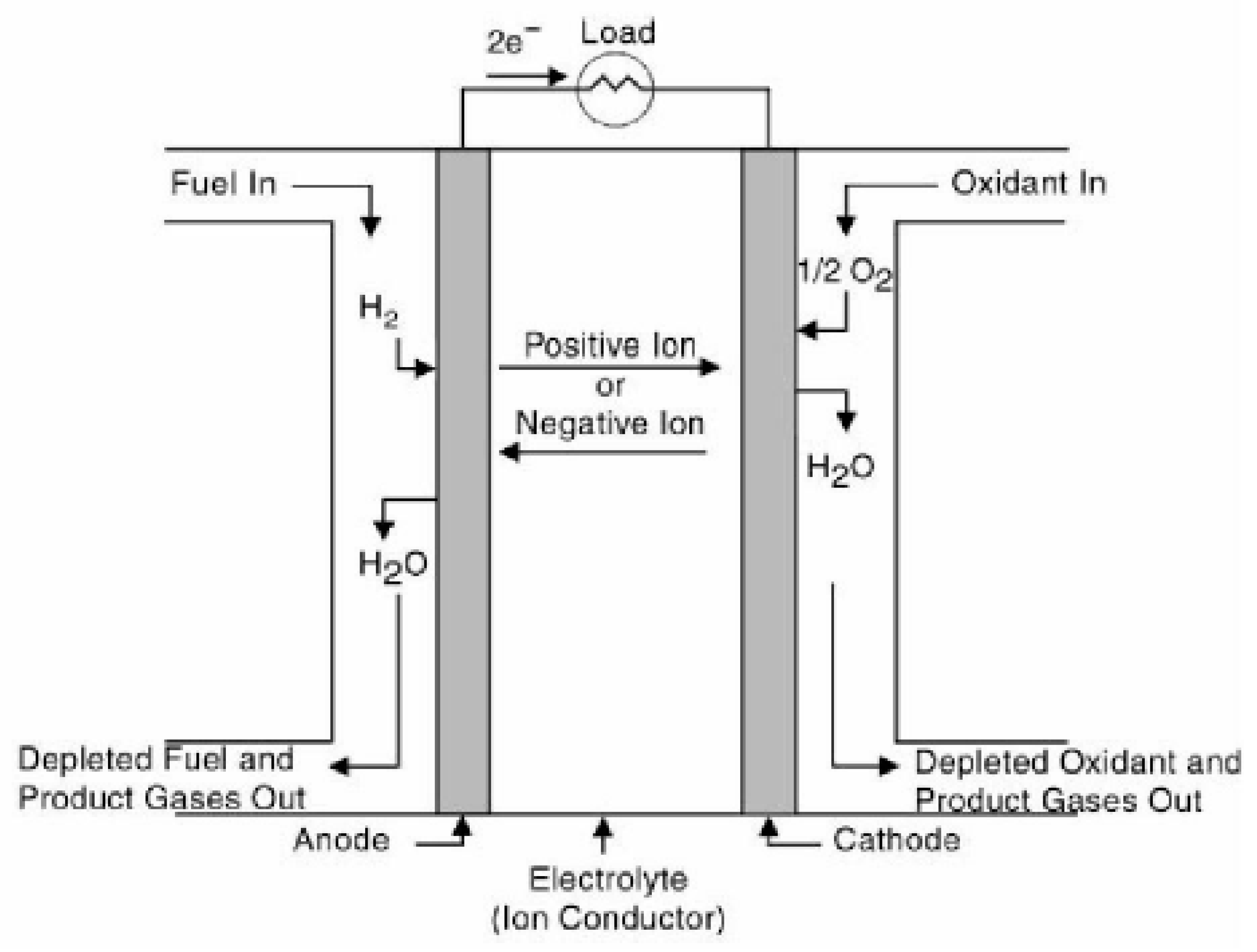
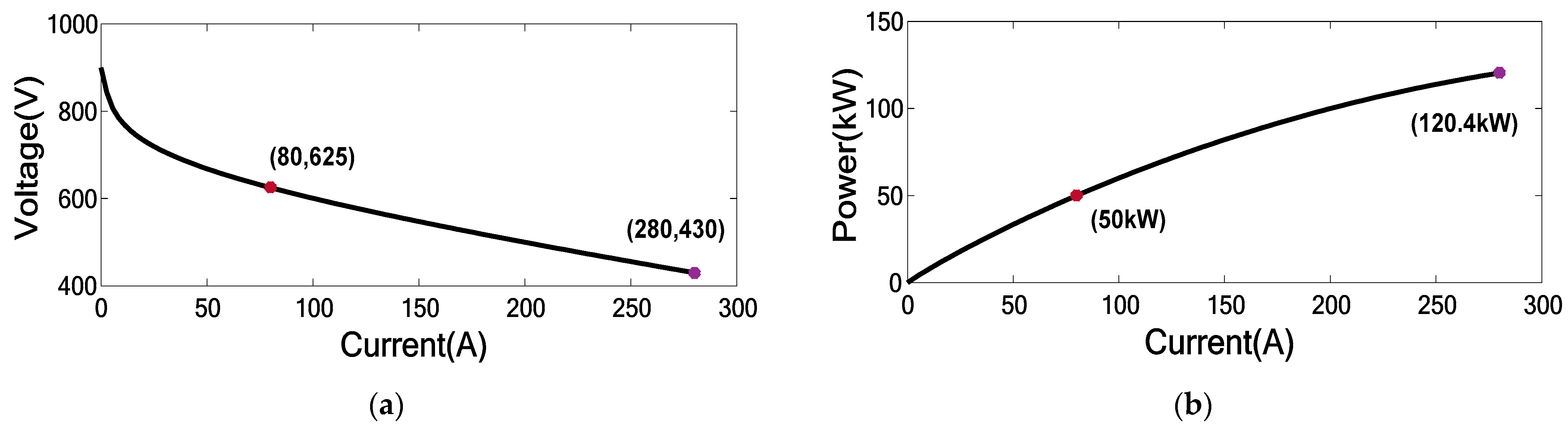
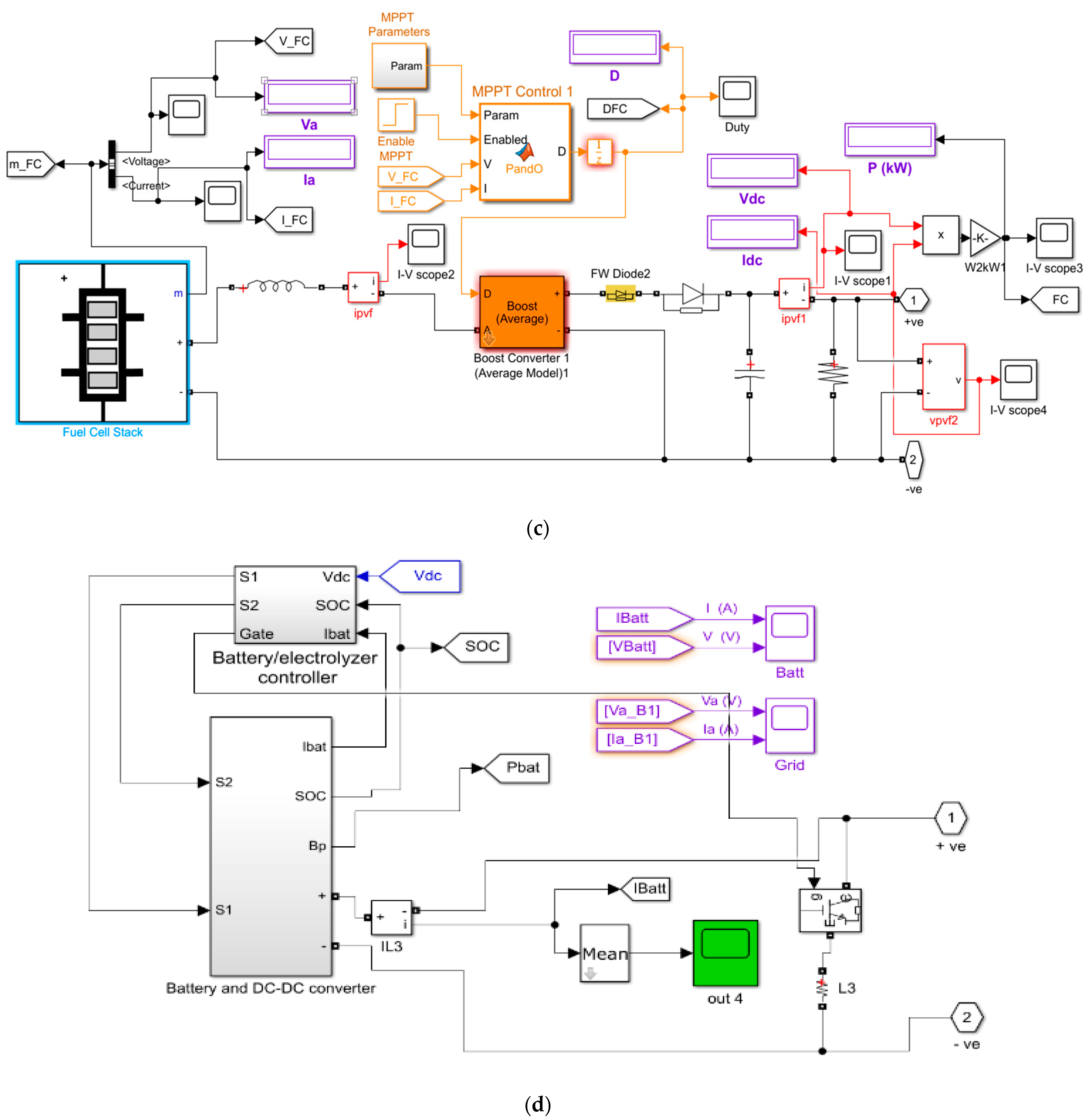
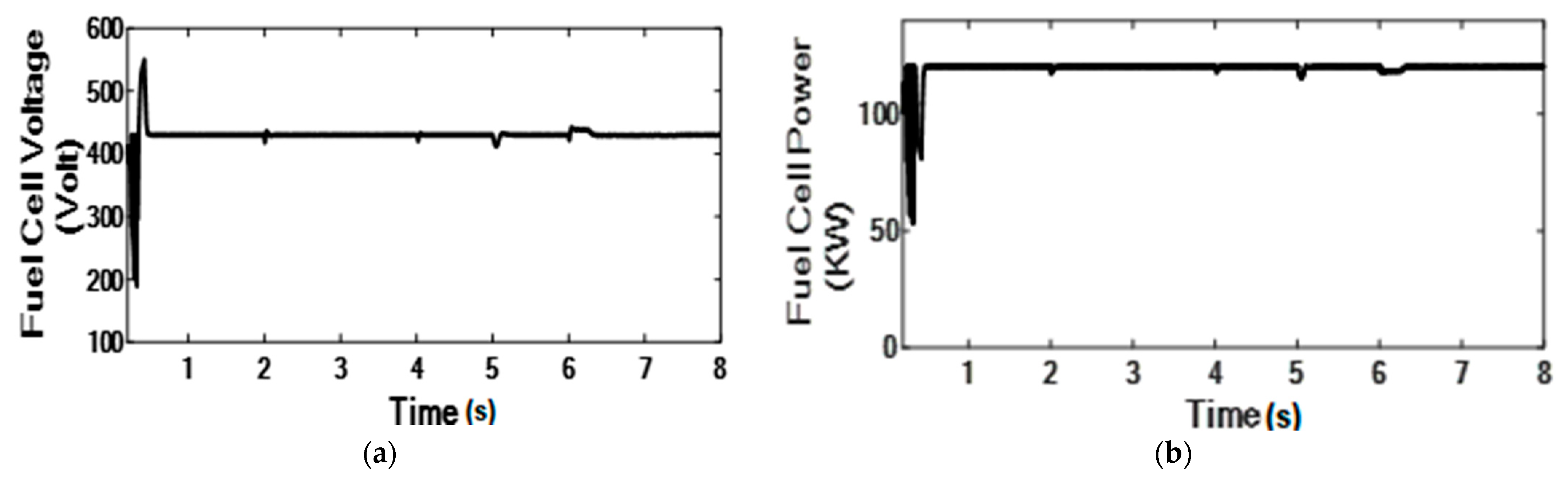
2.3. Modeling of FC System
2.4. Modeling of the DC/DC Converter
3. Control Strategies
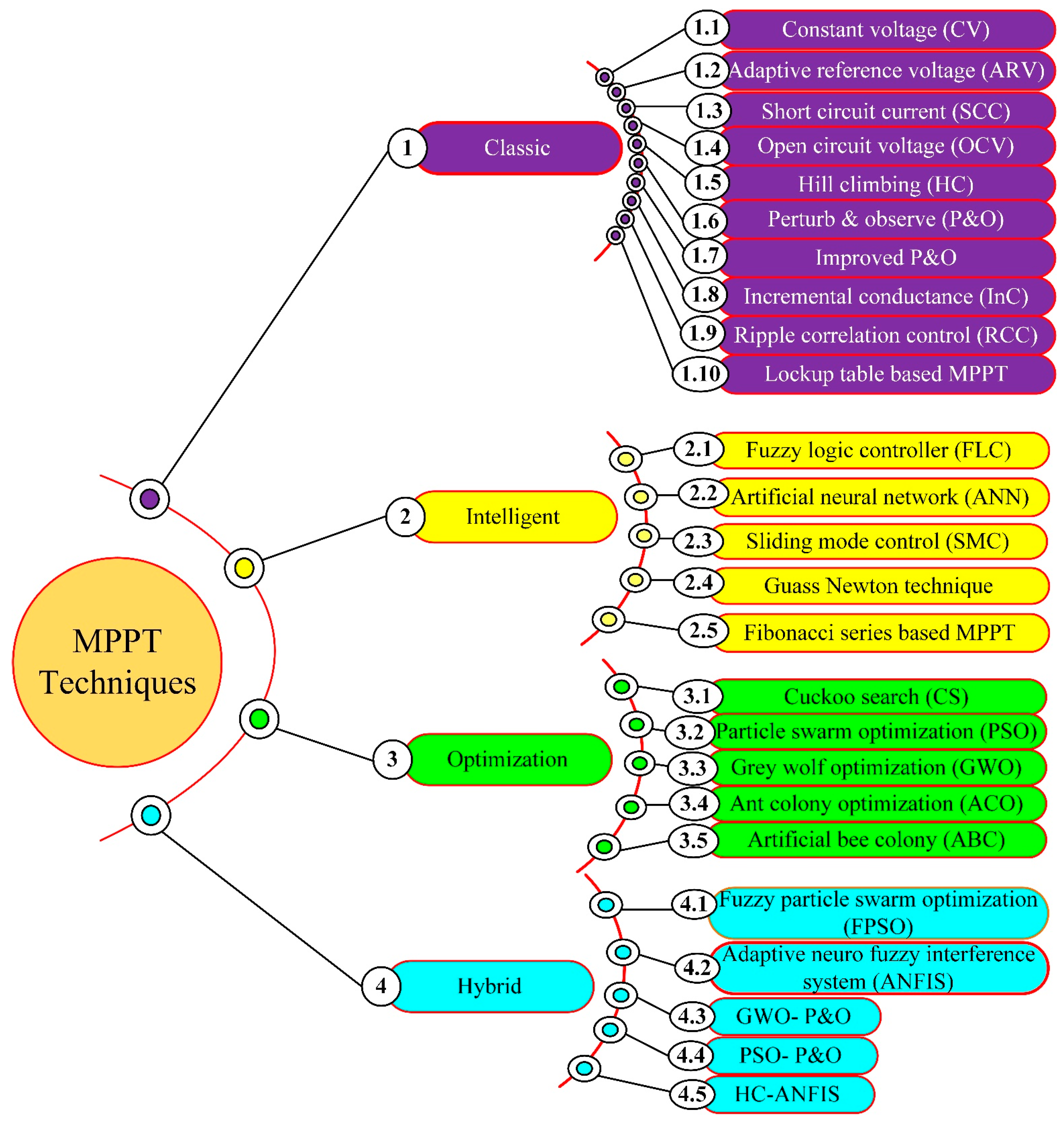
3.1. MPPT Techniques of RES
- A.
- Perturb and observe (P and O) technique
- B.
- Incremental conductance technique (inc. cond.)
- C.
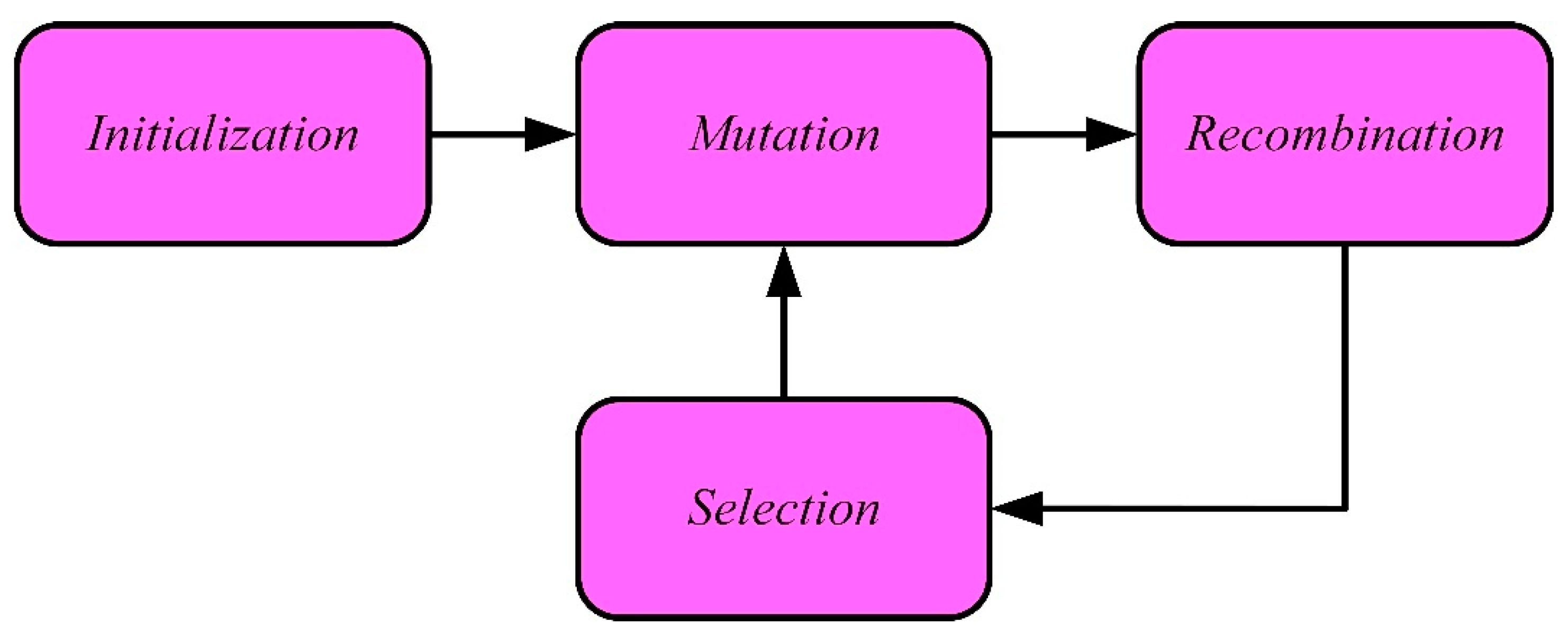
- Differential evolution technique
- D.
- Antlion optimization technique
- E.
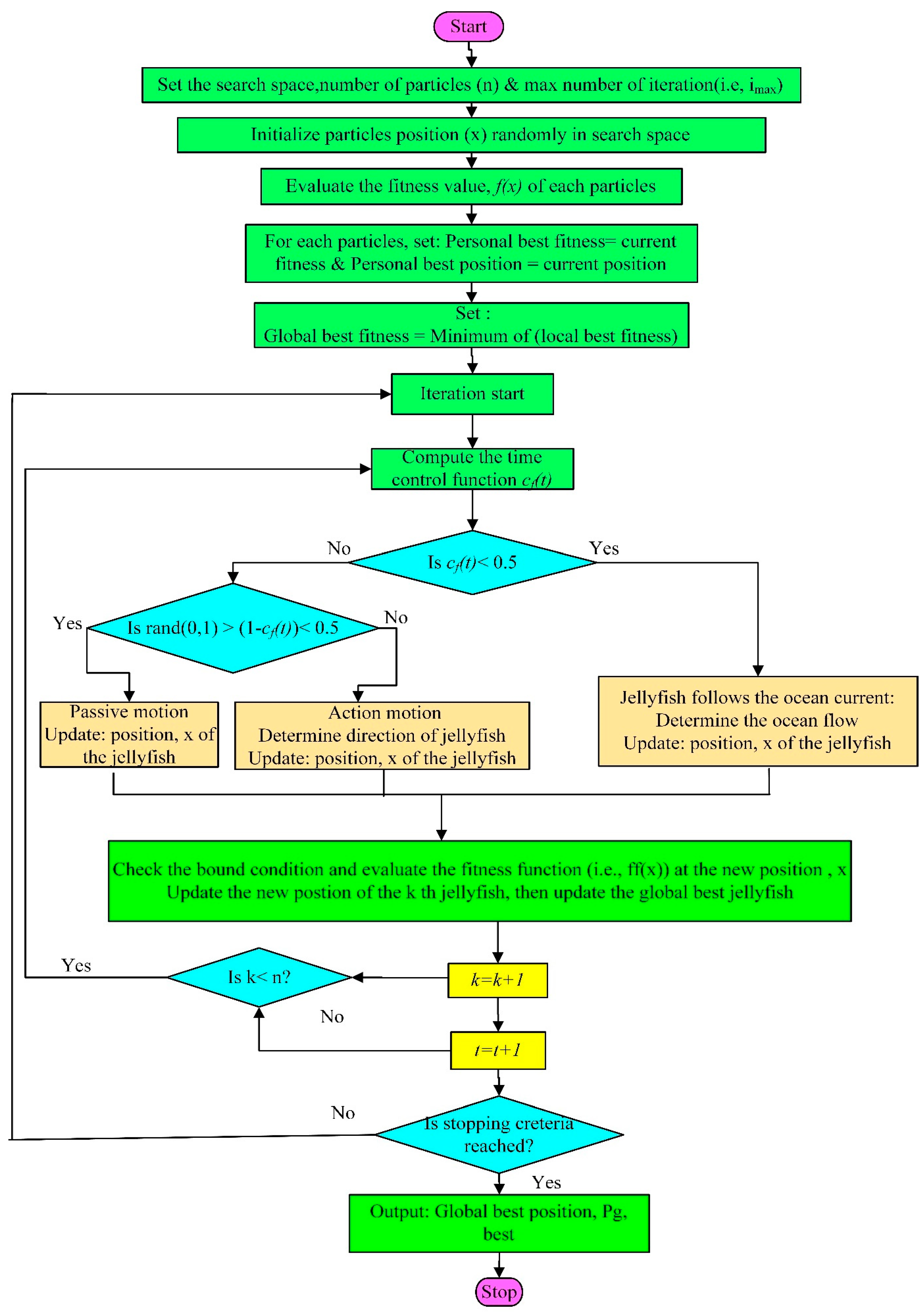
- Bio-inspired jellyfish search optimization
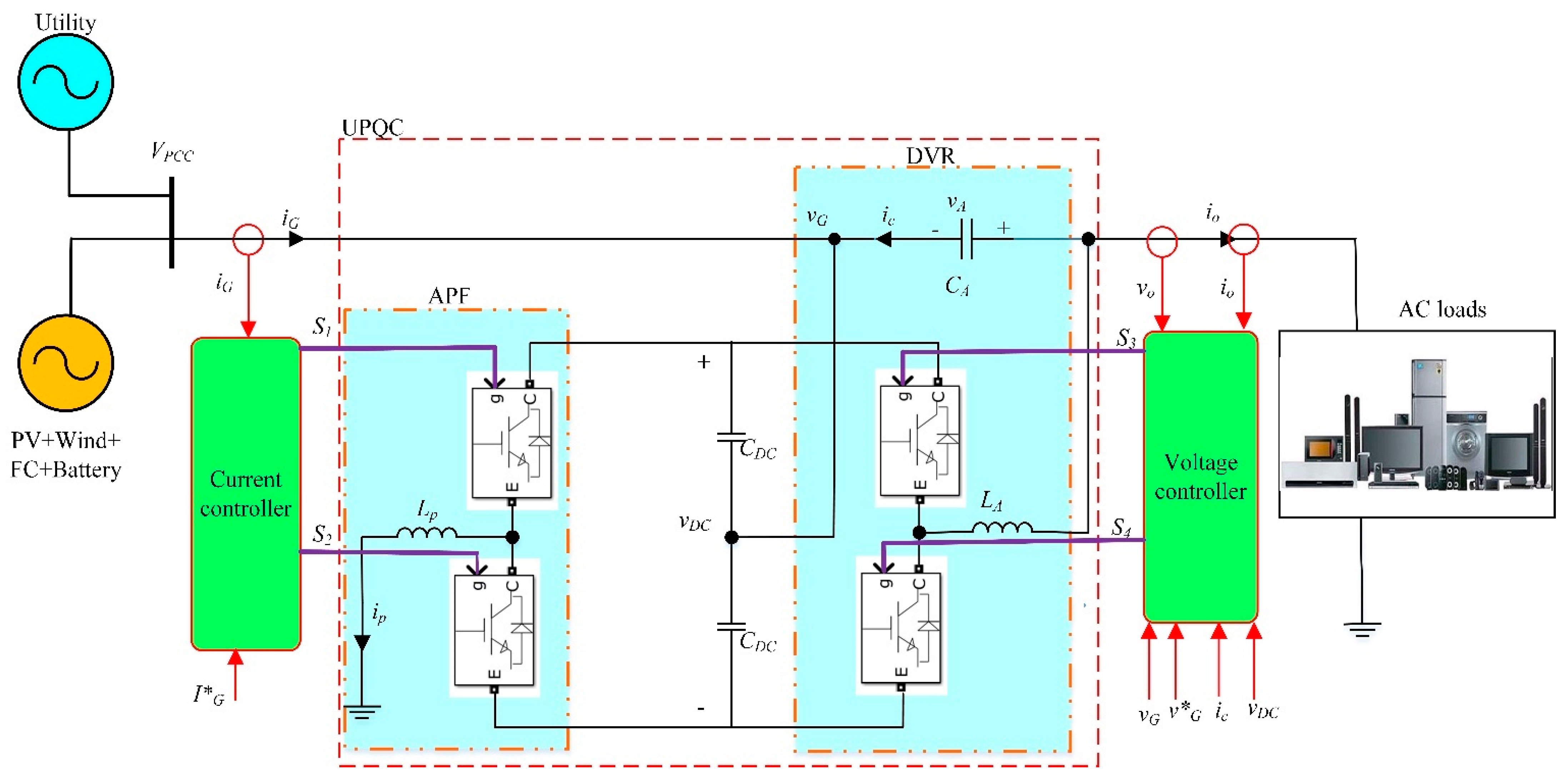
3.2. The Proposed UPQC Topology
- The output voltage controller maintains a constant amplitude sinusoidal output voltage and quickly responds to transients such as grid voltage fluctuations.
- The input current controller maintains the sinusoidal and in-phase grid current.
- The DC-link voltage controller maintains the DC-link voltage between two VSCs, ensuring an optimal balance between input power and output power.
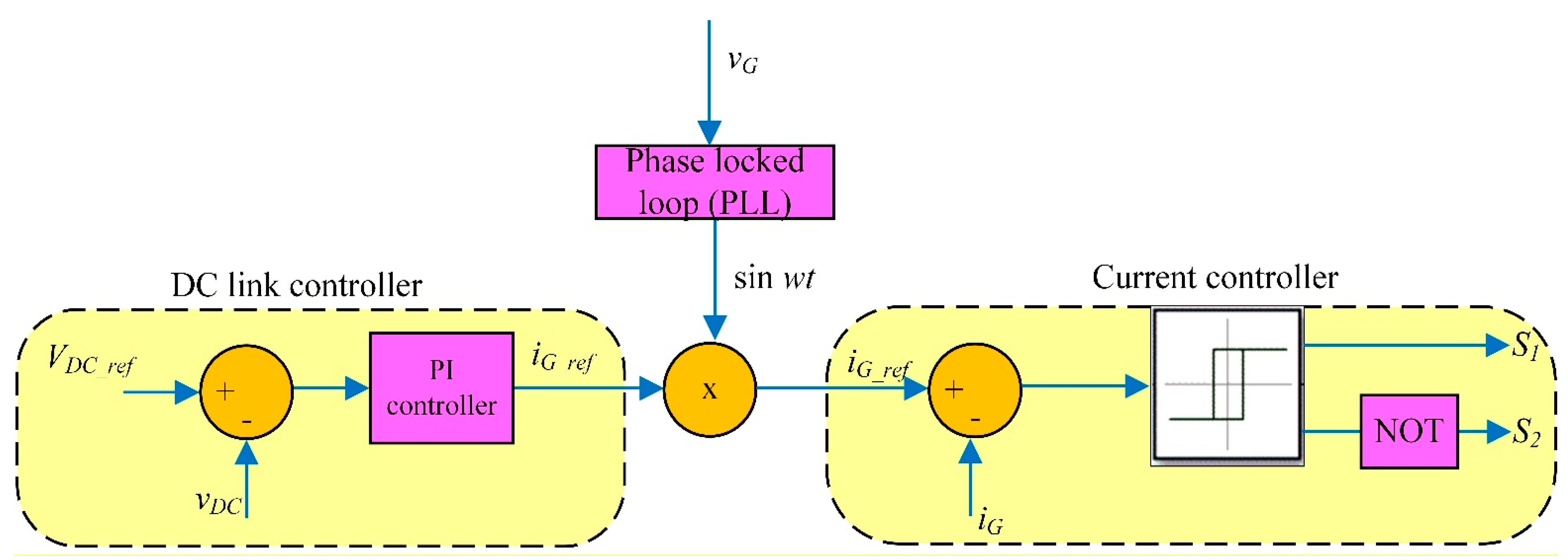
3.2.1. Control Method of APF
3.2.2. Control Method of DVR
4. Simulation Results
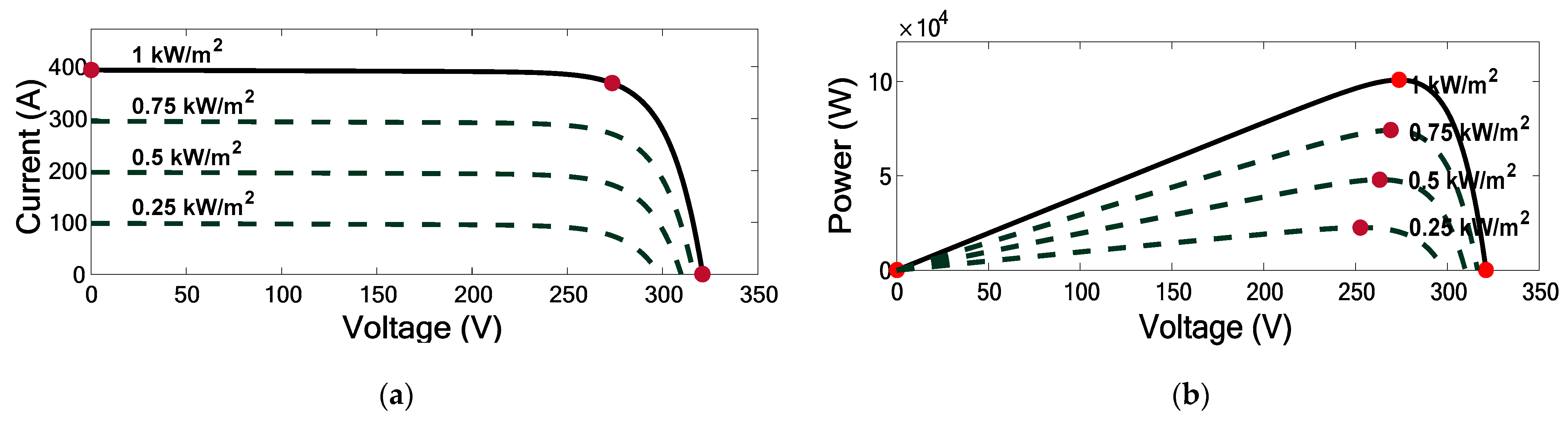
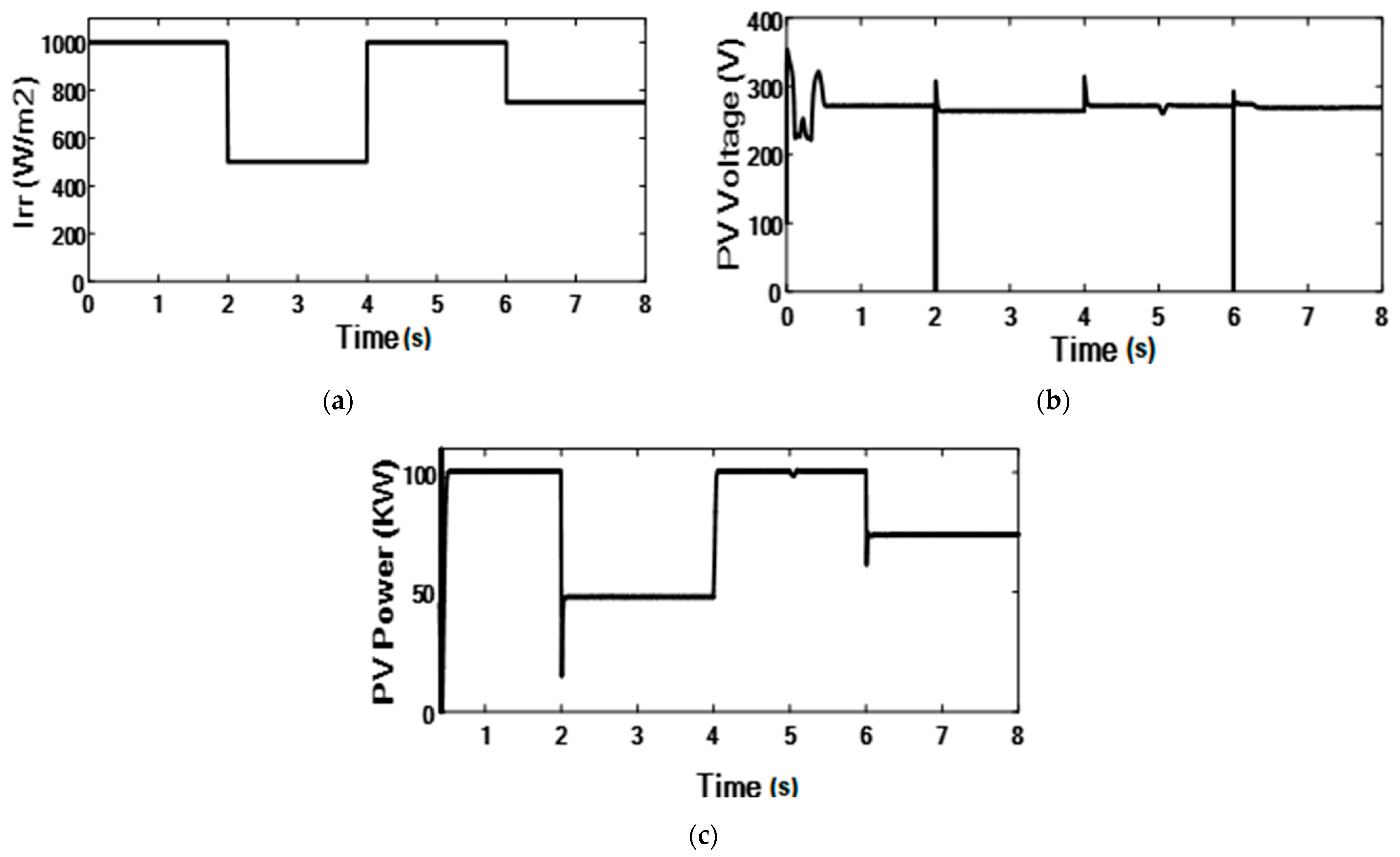
4.1. Reliability and Feasibility of the MPPT Technique during Changes in Climate Conditions
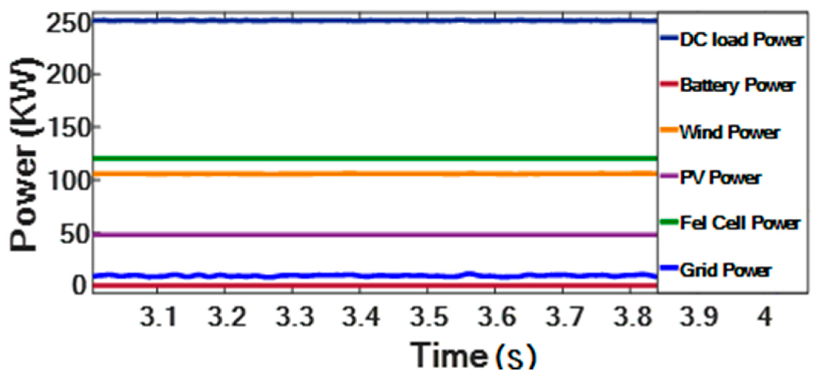
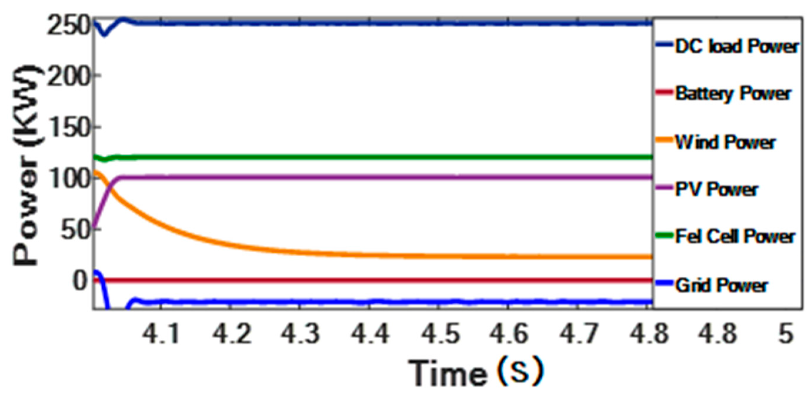
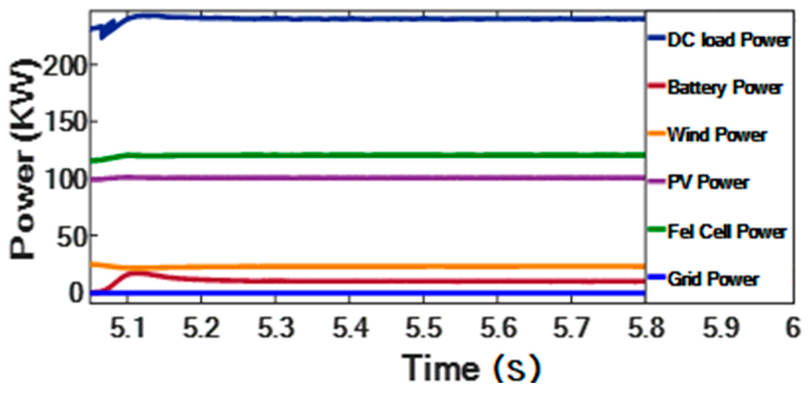
4.2. Dynamic Response of the Proposed Scheme
- (A)
- First sample during the time interval from 3 to 4 s
- (B)
- Second sample during the time interval from 4 to 5 s
- (C)
- Third sample during the time interval from 5 to 6 s
- (D)
- Comparative study
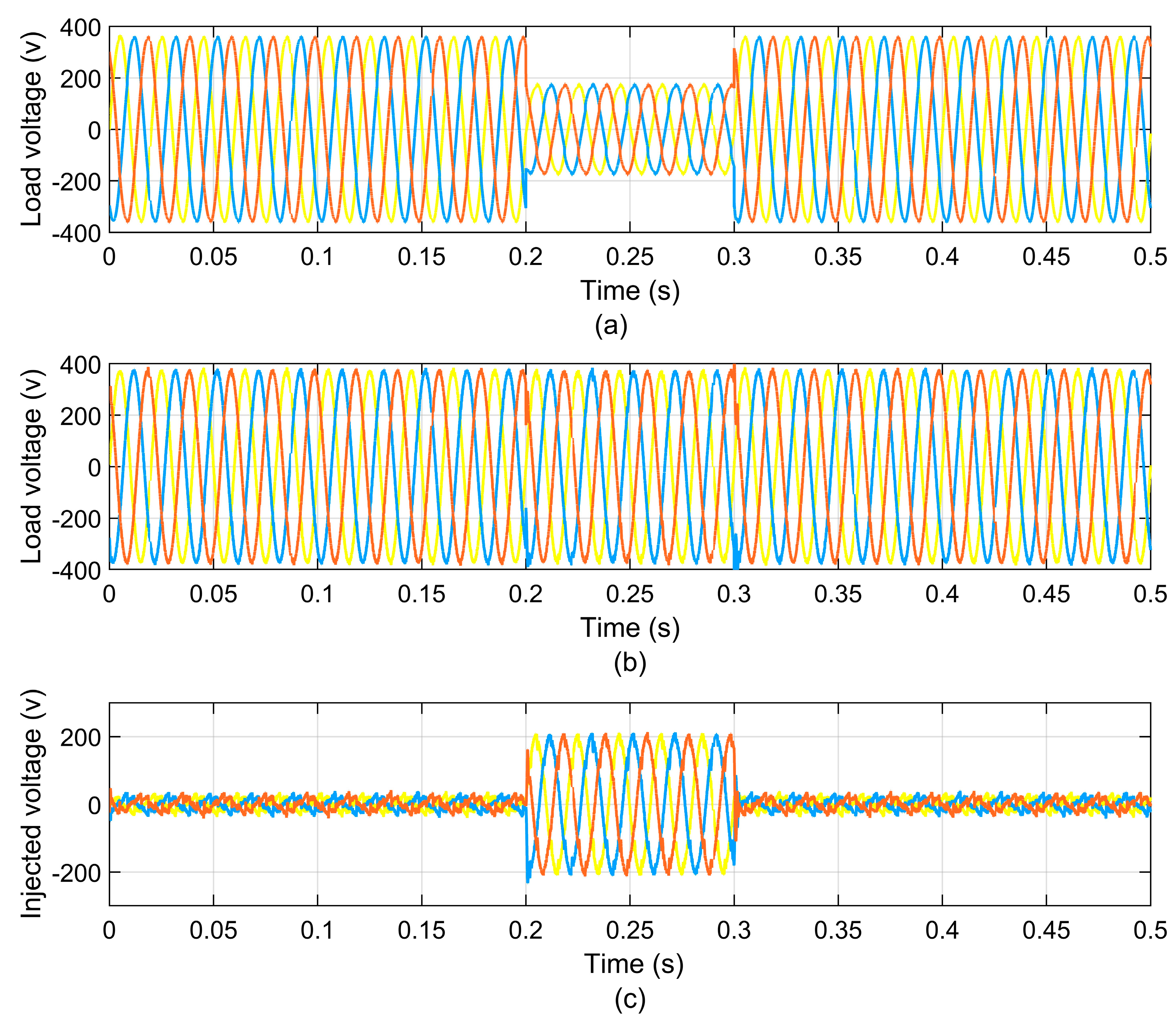
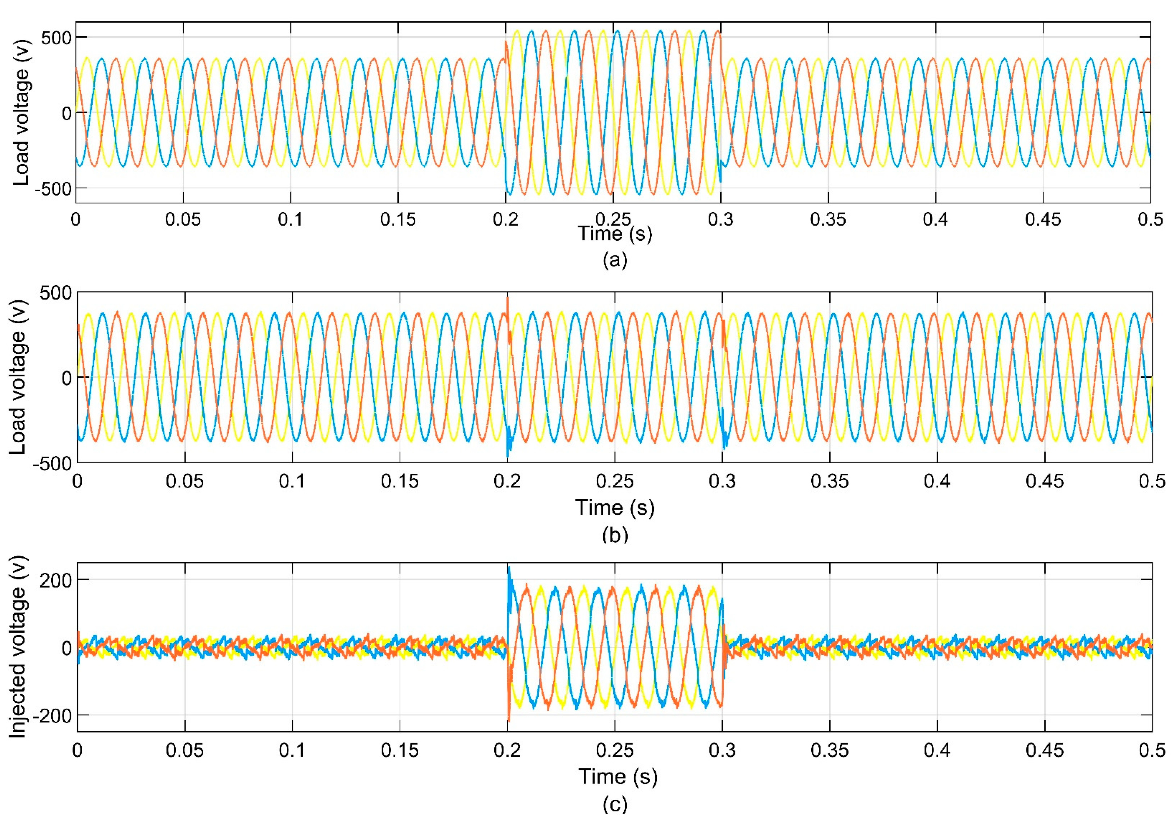
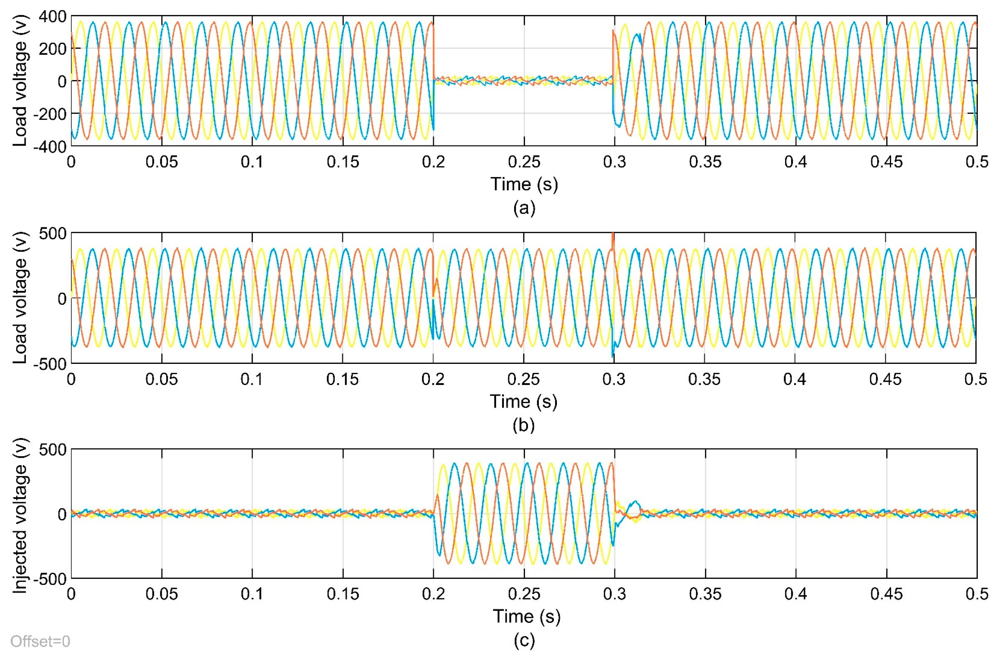
4.3. UPQC Case Studies
- (A)
- Case I: Voltage sag
- (B)
- Case II: Voltage swell
- (C)
- Case III: Three-phase fault
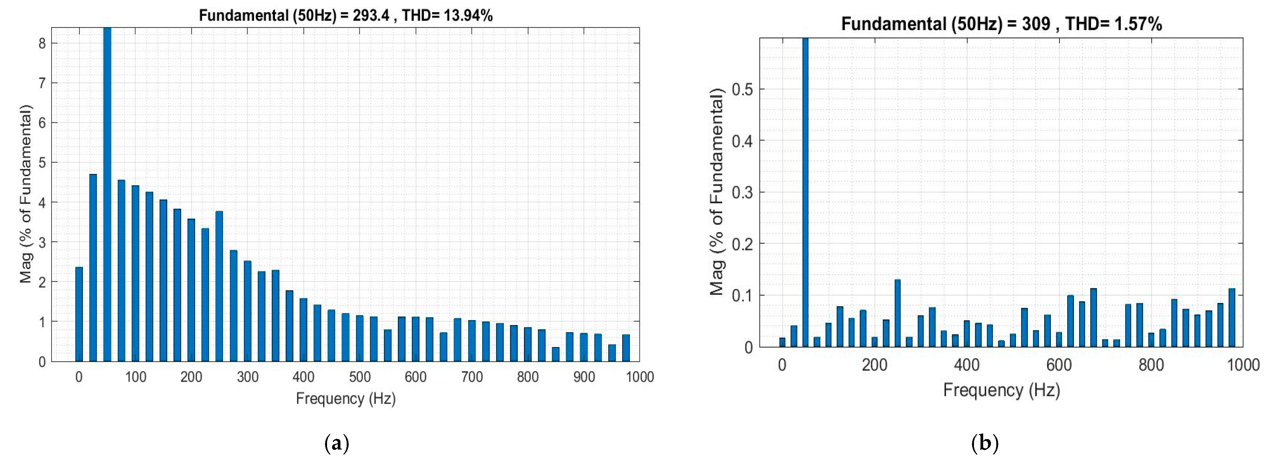
- (D)
- Case IV: Analysis of harmonic distortion
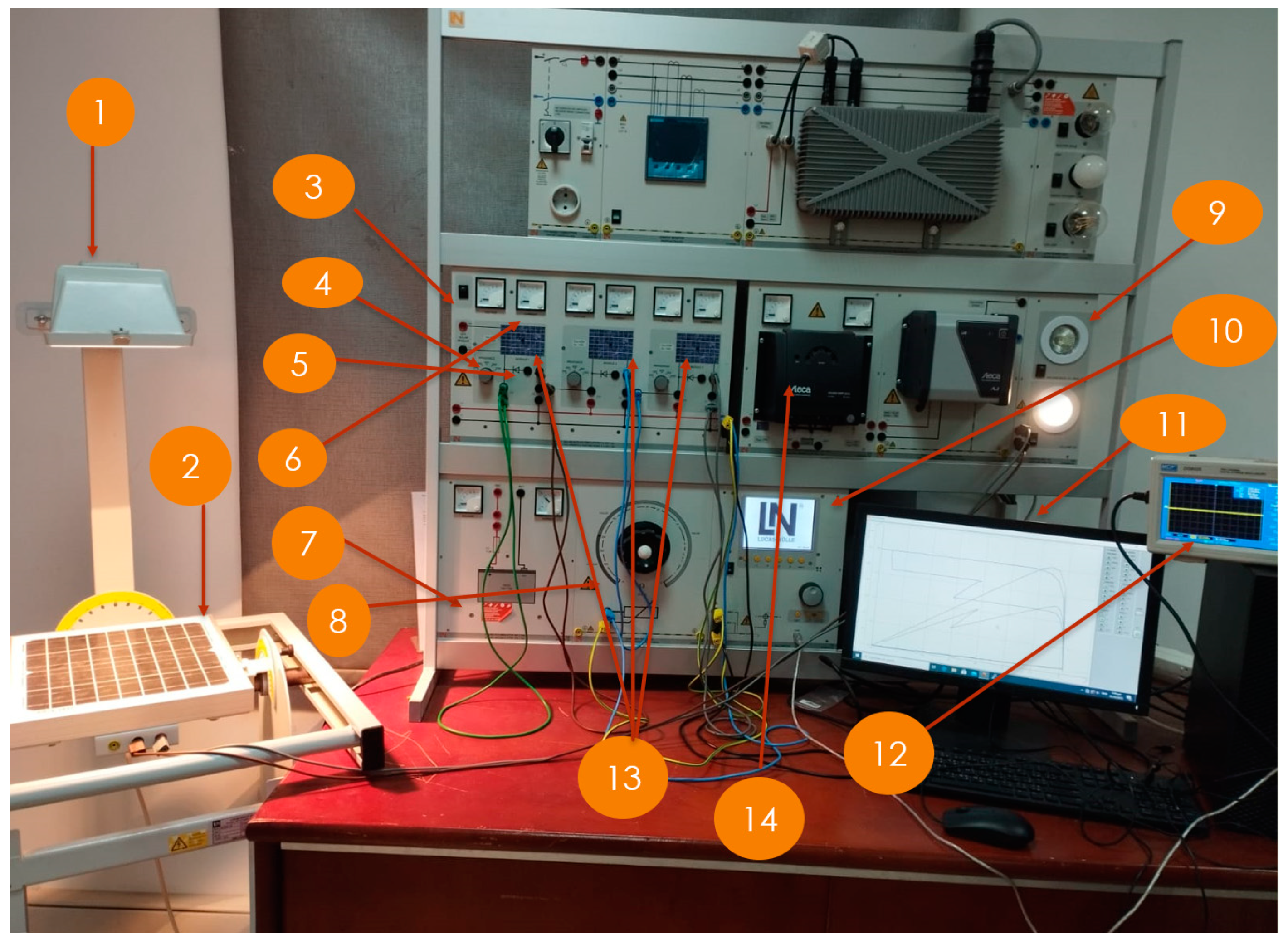
5. Experimental Setup
6. Conclusions
Author Contributions
Funding
Data Availability Statement
Acknowledgments
Conflicts of Interest
References
- Holechek, J.L.; Geli, H.M.E.; Sawalhah, M.N.; Valdez, R. A Global Assessment: Can Renewable Energy Replace Fossil Fuels by 2050? Sustainability 2022, 14, 4792. [Google Scholar] [CrossRef]
- Mahmoud, M.M.; Atia, B.S.; Abdelaziz, A.Y.; Aldin, N.A.N. Dynamic Performance Assessment of PMSG and DFIG-Based WECS with the Support of Manta Ray Foraging Optimizer Considering MPPT, Pitch Control, and FRT Capability Issues. Processes 2022, 12, 2723. [Google Scholar] [CrossRef]
- Halkos, G.E.; Gkampoura, E.C. Reviewing Usage, Potentials, and Limitations of Renewable Energy Sources. Energies 2020, 13, 2906. [Google Scholar] [CrossRef]
- Mahmoud, M.M.; Atia, B.S.; Esmail, Y.M.; Bajaj, M.; Eutyche, D.; Wapet, M.; Ratib, M.K.; Hossain, B.; Aboras, K.M. Evaluation and Comparison of Different Methods for Improving Fault Ride-Through Capability in Grid-Tied Permanent Magnet Synchronous Wind Generators. Int. Trans. Electr. Energy Syst. 2023, 2023, 7717070. [Google Scholar] [CrossRef]
- Al-Majidi, S.D.; Abbod, M.F.; Al-Raweshidy, H.S. A Novel Maximum Power Point Tracking Technique Based on Fuzzy Logic for Photovoltaic Systems. Int. J. Hydrogen Energy 2018, 43, 14158–14171. [Google Scholar] [CrossRef]
- Shafiul Alam, M.; Al-Ismail, F.S.; Salem, A.; Abido, M.A. High-Level Penetration of Renewable Energy Sources into Grid Utility: Challenges and Solutions. IEEE Access 2020, 8, 190277–190299. [Google Scholar] [CrossRef]
- Fateh, D.; Eldoromi, M.; Moti Birjandi, A.A. Uncertainty Modeling of Renewable Energy Sources. In Scheduling and Operation of Virtual Power Plants: Technical Challenges and Electricity Markets; Zangeneh, A., Moeini-Aghtaie, M.B.T.-S., Oof, V.P.P., Eds.; Elsevier: Amsterdam, The Netherlands, 2022; pp. 193–208. ISBN 9780323852685. [Google Scholar]
- Fan, F.; Zhang, R.; Xu, Y.; Ren, S. Robustly Coordinated Operation of an Emission-Free Microgrid with Hybrid Hydrogen-Battery Energy Storage. CSEE J. Power Energy Syst. 2022, 8, 369–379. [Google Scholar] [CrossRef]
- Yoo, Y.; Jung, S.; Jang, G. Dynamic Inertia Response Support by Energy Storage System with Renewable Energy Integration Substation. J. Mod. Power Syst. Clean Energy 2020, 8, 260–266. [Google Scholar] [CrossRef]
- Younis, R.A.; Ibrahim, D.K.; Aboul-Zahab, E.M.; El’Gharably, A. Power Management Regulation Control Integrated with Demand Side Management for Stand-Alone Hybrid Microgrid Considering Battery Degradation. Int. J. Renew. Energy Res. 2019, 9, 1912–1923. [Google Scholar] [CrossRef]
- Aazami, R.; Heydari, O.; Tavoosi, J.; Shirkhani, M.; Mohammadzadeh, A.; Mosavi, A. Optimal Control of an Energy-Storage System in a Microgrid for Reducing Wind-Power Fluctuations. Sustainability 2022, 14, 6183. [Google Scholar] [CrossRef]
- Elmetwaly, A.H.; ElDesouky, A.A.; Omar, A.I.; Attya Saad, M. Operation Control, Energy Management, and Power Quality Enhancement for a Cluster of Isolated Microgrids. Ain Shams Eng. J. 2022, 13, 101737. [Google Scholar] [CrossRef]
- Elmetwaly, A.H.; Eldesouky, A.A.; Sallam, A.A. An Adaptive D-FACTS for Power Quality Enhancement in an Isolated Microgrid. IEEE Access 2020, 8, 57923–57942. [Google Scholar] [CrossRef]
- Mahmoud, M.M. Improved Current Control Loops in Wind Side Converter with the Support of Wild Horse Optimizer for Enhancing the Dynamic Performance of PMSG- Based Wind Generation System. Int. J. Model. Simul. 2022, 1–15. [Google Scholar] [CrossRef]
- Li, X.; Wang, Q.; Wen, H.; Xiao, W. Comprehensive Studies on Operational Principles for Maximum Power Point Tracking in Photovoltaic Systems. IEEE Access 2019, 7, 121407–121420. [Google Scholar] [CrossRef]
- Mao, M.; Cui, L.; Zhang, Q.; Guo, K.; Zhou, L.; Huang, H. Classification and Summarization of Solar Photovoltaic MPPT Techniques: A Review Based on Traditional and Intelligent Control Strategies. Energy Rep. 2020, 6, 1312–1327. [Google Scholar] [CrossRef]
- Hanzaei, S.H.; Gorji, S.A.; Ektesabi, M. A Scheme-Based Review of MPPT Techniques with Respect to Input Variables Including Solar Irradiance and PV Arrays’ Temperature. IEEE Access 2020, 8, 182229–182239. [Google Scholar] [CrossRef]
- Verma, D.; Nema, S.; Shandilya, A.M.; Dash, S.K. Maximum Power Point Tracking (MPPT) Techniques: Recapitulation in Solar Photovoltaic Systems. Renew. Sustain. Energy Rev. 2016, 54, 1018–1034. [Google Scholar] [CrossRef]
- Chen, P.C.; Chen, P.Y.; Liu, Y.H.; Chen, J.H.; Luo, Y.F. A Comparative Study on Maximum Power Point Tracking Techniques for Photovoltaic Generation Systems Operating under Fast Changing Environments. Sol. Energy 2015, 119, 261–276. [Google Scholar] [CrossRef]
- Bhukya, L.; Kedika, N.R.; Salkuti, S.R. Enhanced Maximum Power Point Techniques for Solar Photovoltaic System under Uniform Insolation and Partial Shading Conditions: A Review. Algorithms 2022, 15, 365. [Google Scholar] [CrossRef]
- Hadji, S.; Gaubert, J.P.; Krim, F. Theoretical and Experimental Analysis of Genetic Algorithms Based MPPT for PV Systems. Energy Procedia 2015, 74, 772–787. [Google Scholar] [CrossRef]
- Ahmad, R.; Murtaza, A.F.; Sher, H.A. Power Tracking Techniques for Efficient Operation of Photovoltaic Array in Solar Applications—A Review. Renew. Sustain. Energy Rev. 2019, 101, 82–102. [Google Scholar] [CrossRef]
- Islam, H.; Mekhilef, S.; Shah, N.B.M.; Soon, T.K.; Seyedmahmousian, M.; Horan, B.; Stojcevski, A. Performance Evaluation of Maximum Power Point Tracking Approaches and Photovoltaic Systems. Energies 2018, 11, 365. [Google Scholar] [CrossRef]
- Podder, A.K.; Roy, N.K.; Pota, H.R. MPPT Methods for Solar PV Systems: A Critical Review Based on Tracking Nature. IET Renew. Power Gener. 2019, 13, 1615–1632. [Google Scholar] [CrossRef]
- Seyedmahmoudian, M.; Horan, B.; Soon, T.K.; Rahmani, R.; Than Oo, A.M.; Mekhilef, S.; Stojcevski, A. State of the Art Artificial Intelligence-Based MPPT Techniques for Mitigating Partial Shading Effects on PV Systems—A Review. Renew. Sustain. Energy Rev. 2016, 64, 435–455. [Google Scholar] [CrossRef]
- Fathi, M.; Parian, J.A. Intelligent MPPT for Photovoltaic Panels Using a Novel Fuzzy Logic and Artificial Neural Networks Based on Evolutionary Algorithms. Energy Rep. 2021, 7, 1338–1348. [Google Scholar] [CrossRef]
- Belay Kebede, A.; Biru Worku, G. Comprehensive Review and Performance Evaluation of Maximum Power Point Tracking Algorithms for Photovoltaic System. Glob. Energy Interconnect. 2020, 3, 398–412. [Google Scholar] [CrossRef]
- Ibrahim, A.W.; Shafik, M.B.; Ding, M.; Sarhan, M.A.; Fang, Z.; Alareqi, A.G.; Almoqri, T.; Al-Rassas, A.M. PV Maximum Power-Point Tracking Using Modified Particle Swarm Optimization under Partial Shading Conditions. Chin. J. Electr. Eng. 2020, 6, 106–121. [Google Scholar] [CrossRef]
- Zhao, Z.; Zhang, M.; Zhang, Z.; Wang, Y.; Cheng, R.; Guo, J.; Yang, P.; Lai, C.S.; Li, P.; Lai, L.L. Hierarchical Pigeon-Inspired Optimization-Based MPPT Method for Photovoltaic Systems Under Complex Partial Shading Conditions. IEEE Trans. Ind. Electron. 2022, 69, 10129–10143. [Google Scholar] [CrossRef]
- Zhang, X.; Gamage, D.; Wang, B.; Ukil, A. Hybrid Maximum Power Point Tracking Method Based on Iterative Learning Control and Perturb & Observe Method. IEEE Trans. Sustain. Energy 2021, 12, 659–670. [Google Scholar] [CrossRef]
- Mohapatra, A.; Nayak, B.; Das, P.; Mohanty, K.B. A Review on MPPT Techniques of PV System under Partial Shading Condition. Renew. Sustain. Energy Rev. 2017, 80, 854–867. [Google Scholar] [CrossRef]
- Nazaripouya, H.; Mehraeen, S. Modeling and Nonlinear Optimal Control of Weak/Islanded Grids Using FACTS Device in a Game Theoretic Approach. IEEE Trans. Control Syst. Technol. 2016, 24, 158–171. [Google Scholar] [CrossRef]
- Ochoa-Giménez, M.; García-Cerrada, A.; Zamora-Macho, J.L. Comprehensive Control for Unified Power Quality Conditioners. J. Mod. Power Syst. Clean. Energy 2017, 5, 609–619. [Google Scholar] [CrossRef]
- Bouloumpasis, I.; Vovos, P.; Georgakas, K.; Vovos, N.A. Current Harmonics Compensation in Microgrids Exploiting the Power Electronics Interfaces of Renewable Energy Sources. Energies 2015, 8, 2295–2311. [Google Scholar] [CrossRef]
- Tey, K.S.; Mekhilef, S.; Seyedmahmoudian, M.; Horan, B.; Oo, A.T.; Stojcevski, A. Improved Differential Evolution-Based MPPT Algorithm Using SEPIC for PV Systems Under Partial Shading Conditions and Load Variation. IEEE Trans. Ind. Inform. 2018, 14, 4322–4333. [Google Scholar] [CrossRef]
- Balamurugan, M.; Sahoo, S.K.; Sukchai, S. Maximum Power Extraction Using Ant Lion Optimization Technique for Photovoltaic System. In Proceedings of the 3rd IEEE International Virtual Conference on Innovations in Power and Advanced Computing Technologies, i-PACT 2021, Kuala Lumpur, Malaysia, 27–29 November 2021; pp. 1–8. [Google Scholar]
- Chou, J.-S.; Molla, A. Recent Advances in Use of Bio-Inspired Jellyfish Search Algorithm for Solving Optimization Problems. Sci. Rep. 2022, 12, 19157. [Google Scholar] [CrossRef] [PubMed]
- Boutasseta, N.; Bouakkaz, M.S.; Fergani, N.; Attoui, I.; Bouraiou, A.; Neçaibia, A. Solar Energy Conversion Systems Optimization Using Novel Jellyfish Based Maximum Power Tracking Strategy. Procedia Comput. Sci. 2021, 194, 80–88. [Google Scholar] [CrossRef]
- Alam, A.; Verma, P.; Tariq, M.; Sarwar, A.; Alamri, B.; Zahra, N.; Urooj, S. Jellyfish Search Optimization Algorithm for Mpp Tracking of Pv System. Sustainability 2021, 13, 11736. [Google Scholar] [CrossRef]
- Abdel Mohsen, S.E.; Ibrahim, A.M.; Elbarbary, Z.M.S.; Omar, A.I. Unified Power Quality Conditioner Using Recent Optimization Technique: A Case Study in Cairo Airport, Egypt. Sustainability 2023, 15, 3710. [Google Scholar] [CrossRef]


| Equipment | Position | Values |
|---|---|---|
| Transformer (T1) | Between Vg and Vpcc | 1.6/12 kV, 10 MVA |
| FC | Vb | 625 V and 120 kW |
| Battery storage | Vb | 625 V and 5000 Ah |
| PV | Vb | 625 V and 1 MVA |
| Wind turbine | Vb | 1.6 kV and 0.5 MVA |
| AC loads | Vpcc | Linear: 1.6 kV, 675 kW, and 386 kVar |
| Nonlinear: 1.6 kV, 135 kW, and 75 kVar | ||
| DC loads | Vb | 1.6 kV and 185 kW |
| System Powers (kW) | ||||||
|---|---|---|---|---|---|---|
| t (s) | PV | Wind | FC | Load | Battery | Grid |
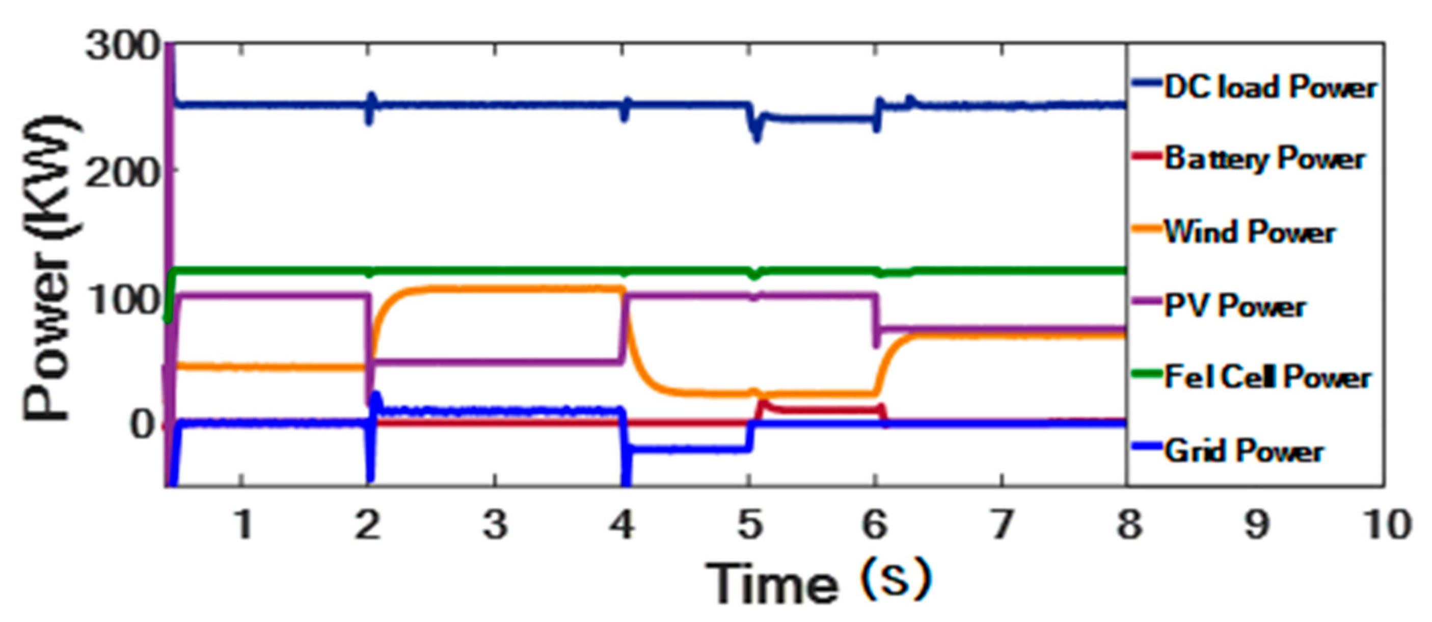
| [3,4] | 48 | 105.3 | 120.3 | 250 | 0 | 10 |
| 273.6 | ||||||
| System Powers (kW) | ||||||
|---|---|---|---|---|---|---|
| t (s) | PV | Wind | FC | Load | Battery | Grid |
| [4,5] | 100.6 | 23.1 | 120.3 | 250 | 0 | −21 |
| 244 | ||||||
| System Powers (kW) | ||||||
|---|---|---|---|---|---|---|
| t (s) | PV | Wind | FC | Load | Battery | Grid |
| [5,6] | 100.6 | 23.1 | 120.3 | 240 | 10 | 0 |
| 244 | ||||||
| Irradiance (kW/m2) | MP (kW) from Figure 3 | P and O | Inc. Cond. | DE | ALO | Proposed JSO | |||||
|---|---|---|---|---|---|---|---|---|---|---|---|
| Power (kW) | Eff. | Power (kW) | Eff. | Power (kW) | Eff. | Power (kW) | Eff. | Power (kW) | Eff. | ||
| 1 | 100.7 | 100.1 | 99.4 | 100.5 | 99.8 | 100.5 | 99.8 | 100.6 | 99.9 | 100.65 | 99.9 |
| 0.75 | 74.2 | 73.7 | 99.4 | 74 | 99.7 | 74 | 99.7 | 74.1 | 99.8 | 74.2 | 99.8 |
| 0.5 | 48.1 | 47.8 | 99.3 | 47.9 | 99.5 | 47.8 | 99.3 | 48 | 99.7 | 48.1 | 99.9 |
| Wind Speed (m/s) | MP (kW) from Figure 4 | P and O | Inc. Cond. | DE | ALO | Proposed JSO | |||||
|---|---|---|---|---|---|---|---|---|---|---|---|
| Power (kW) | Eff. | Power (kW) | Eff. | Power (kW) | Eff. | Power (kW) | Eff. | Power (kW) | Eff. | ||
| 12 | 105.4 | 104.8 | 99.4 | 105 | 99.6 | 104.8 | 99.4 | 105.3 | 99.9 | 105.4 | 99.9 |
| 11 | 68.4 | 67.8 | 99.1 | 67.9 | 99.2 | 67.8 | 99.1 | 68.1 | 99.5 | 68.2 | 99.6 |
| 10 | 44.4 | 43.9 | 98.8 | 44 | 99 | 44 | 99 | 44.1 | 99.4 | 44.3 | 99.8 |
| 9 | 23.2 | 22.8 | 98.4 | 22.8 | 98.9 | 23 | 99.1 | 23.1 | 99.4 | 23.1 | 99.4 |
| MP from Figure 6 | P and O | Inc. Cond. | DE | ALO | Proposed JSO | |||||
|---|---|---|---|---|---|---|---|---|---|---|
| Power | Eff. | Power | Eff. | Power | Eff. | Power | Eff. | Power | Eff. | |
| 120.4 | 120.2 | 99.8 | 120.2 | 99.8 | 120.2 | 99.8 | 120.3 | 99.9 | 120.3 | 99.9 |
| Algorithm | Energy Source | Algorithm Complexity | Memory Requirement | Convergence Speed | Response to Climate Changes |
|---|---|---|---|---|---|
| P and O | PV Wind FC | Less Less Less | Less Less Less | Less Moderate Less | Less Moderate Less |
| Inc. Cond. | PV Wind FC | Less Less Less | Less Less Less | Less Moderate Less | Less Moderate Less |
| DE | PV Wind FC | High High High | High High High | High High High | High High High |
| ALO | PV Wind FC | High High High | High High High | High High High | High High High |
| Proposed JSO | PV Wind FC | High High High | High High High | High High High | High High High |
| Specifications | Values |
|---|---|
| Nominal AC- and DC-link voltages | 400 V, 50 Hz |
| 10 mH | |
| 3.4 mH | |
| 14.1 μF | |
| 1500 μF |
Disclaimer/Publisher’s Note: The statements, opinions and data contained in all publications are solely those of the individual author(s) and contributor(s) and not of MDPI and/or the editor(s). MDPI and/or the editor(s) disclaim responsibility for any injury to people or property resulting from any ideas, methods, instructions or products referred to in the content. |
© 2023 by the authors. Licensee MDPI, Basel, Switzerland. This article is an open access article distributed under the terms and conditions of the Creative Commons Attribution (CC BY) license (https://creativecommons.org/licenses/by/4.0/).
Share and Cite
Elmetwaly, A.H.; Younis, R.A.; Abdelsalam, A.A.; Omar, A.I.; Mahmoud, M.M.; Alsaif, F.; El-Shahat, A.; Saad, M.A. Modeling, Simulation, and Experimental Validation of a Novel MPPT for Hybrid Renewable Sources Integrated with UPQC: An Application of Jellyfish Search Optimizer. Sustainability 2023, 15, 5209. https://doi.org/10.3390/su15065209
Elmetwaly AH, Younis RA, Abdelsalam AA, Omar AI, Mahmoud MM, Alsaif F, El-Shahat A, Saad MA. Modeling, Simulation, and Experimental Validation of a Novel MPPT for Hybrid Renewable Sources Integrated with UPQC: An Application of Jellyfish Search Optimizer. Sustainability. 2023; 15(6):5209. https://doi.org/10.3390/su15065209
Chicago/Turabian StyleElmetwaly, Ahmed Hussain, Ramy Adel Younis, Abdelazeem Abdallah Abdelsalam, Ahmed Ibrahim Omar, Mohamed Metwally Mahmoud, Faisal Alsaif, Adel El-Shahat, and Mohamed Attya Saad. 2023. "Modeling, Simulation, and Experimental Validation of a Novel MPPT for Hybrid Renewable Sources Integrated with UPQC: An Application of Jellyfish Search Optimizer" Sustainability 15, no. 6: 5209. https://doi.org/10.3390/su15065209
APA StyleElmetwaly, A. H., Younis, R. A., Abdelsalam, A. A., Omar, A. I., Mahmoud, M. M., Alsaif, F., El-Shahat, A., & Saad, M. A. (2023). Modeling, Simulation, and Experimental Validation of a Novel MPPT for Hybrid Renewable Sources Integrated with UPQC: An Application of Jellyfish Search Optimizer. Sustainability, 15(6), 5209. https://doi.org/10.3390/su15065209