Gap Filling Method and Estimation of Net Ecosystem CO₂ Exchange in Alpine Wetland of Qinghai–Tibet Plateau

Abstract

The net ecosystem CO₂ exchange (NEE) and water and energy fluxes at the alpine ecosystem level were obtained through the eddy covariance technique in an alpine wetland of the Longbao Region, Qinghai–Tibet Plateau. Our research used the NEE as the research object combined with meteorological factors. The NEE prediction model was constructed using Reddyproc and machine learning. Moreover, the effects of the data and features on the models and the selection of the model parameters were discussed. The results revealed the following information: (1) After removing the NEE outliers according to the friction wind speed thresholds of the different seasons, the NEE interpolation accuracy (R²) reached 0.65. Additionally, the NEE data dispersion decreased after removing the outliers, and the data quality improved effectively. (2) The decision coefficients (R²) of the eight kinds of combined machine learning algorithm models varied from 0.22 to 0.62, and the root mean square error (RMSE) ranged from 2.10 to 2.99 μmol s⁻¹ m⁻². Additionally, the multilayer perceptron (MLP) model had the best stability and the best interpolation effect. (3) There was a seasonal difference between the estimated values of Reddyproc and the estimated values of MLP. The monthly mean values of January, February, March, and October were lower than the monthly mean values of the latter, while the monthly mean values from April to September were higher than the monthly mean values of the latter, indicating that the prediction of the machine learning algorithm tends towards the carbon source in the cold season (nongrowing season) and tends towards the carbon sink in the warm season (growing season). (4) Reddyproc detected the outliers through the relationship between the night NEE and frictional wind speed, which made it possible to accurately estimate the nighttime flux under the condition of determining the threshold of the night frictional wind speed, thus obtaining a better NEE estimate with fewer input parameters. Before the training and prediction of the MLP model, the NEE was detected for the time series outliers, and the prediction accuracy was significantly improved, indicating that the elimination of the time series outliers is essential for NEE model training and further indicating that the understanding of the potential mechanism of the NEE is of great significance for the prediction model.

1. Introduction

The carbon cycle of terrestrial ecosystems is the core of the material and energy cycles of these ecosystems and is the key process driving ecosystem change [1]. Hence, the quantitative assessment of the carbon budget is an important task in the study of ecosystems and global climate change [2,3]. Net ecosystem exchange (NEE) refers to the change in ecosystem carbon storage caused by plant photosynthesis, the carbon storage in the canopy air, and the carbon emissions from both biotic and abiotic respiration. It mainly reflects the carbon budget of an ecosystem and determines the transition process of the “Sink-source” or “Source-sink” of a surface ecosystem from the perspective of flux observation [4]. As an important part of the Earth’s ecosystem, terrestrial ecosystems are not only the foundation of human survival and development but also play an important role in the global carbon cycle [5]. An accurate assessment of the carbon budget of terrestrial ecosystems not only provides a theoretical basis for understanding and predicting global climate change but also provides a scientific basis for the government to make relevant decisions to reduce greenhouse gas emissions and promote social sustainable development.

The Qinghai–Tibet Plateau ecosystems grow in extremely harsh environments characterized by a low annual average temperature and low rainfall, a high solar radiation and wind speed, a limited availability of soil nutrients and water, and short growing seasons. Therefore, these alpine ecosystems are extremely fragile and sensitive to climate change. Accurately measuring and estimating the carbon flux of the alpine ecosystems in the Qinghai–Tibet Plateau under the background of climate change is crucial for the study of the ecosystem carbon balance.

With the development of energy exchange and mass transfer and the urgent demand for carbon emission reduction, the observation of the NEE has been paid more attention by scholars through research. The vorticity covariance method is one of the most effective methods for measuring the carbon budget between the atmosphere and various ecosystems since the 1980s [6,7]. It has been widely used to measure the exchange of matter and energy between the atmosphere and the Earth’s surface [6,7]. However, in the course of observation, due to various reasons (rainfall, instrument failure, human error operation, etc.) and due to part of the observation data going missing, the CO₂ flux data measured by the flux towers have a high rate of deletion [8]. Nearly 17–50% of the observed data is deleted in a year [8], which brings difficulties to the application of the flux tower data. How to establish an effective and reasonable data interpolation method to form the complete and reliable data integration of CO₂ flux data is a problem to be solved.

Currently, FLUXNET and the European flux network of Carbon Europe use the marginal distribution sampling (MDS) of the mean interpolation method for the interpolation of missing flux data and apply it to the FLUXNET 2015 dataset [9]. OzFlux, the Australian National Ecosystem Research Network, employs an artificial neural network algorithm to interpolate missing flux data [10,11]. However, up to now, the interpolation methods for missing flux data have not been unified among flux networks, and most of them are for the net ecosystem exchange. For example, Moffat [12] systematically discussed the effectiveness of 15 data interpolation methods in the calculation of net ecosystem exchange annual accumulation using 10 sets of observational data from 6 forest sites. The results showed that the selection of an interpolation method has a significant influence on the calculation of annual NEE cumulants and that the uncertainty is about ±25 g·C·m⁻²·y⁻¹. The generalized regression neural network (GRNN) and the extreme learning machine (ELM) proposed by Xianming Dou [13] have a strong nonlinear processing ability to simulate and predict the carbon and water fluxes in terrestrial ecosystems. These models have achieved the highest simulation accuracy in the assessment of the carbon and water fluxes in evergreen coniferous forests and deciduous broad-leaved forests but have given fewer satisfying simulations in cropland ecosystems. Xiaobo Zhu [14] compared the performance of three machine learning models based on a backpropagation artificial neural network (BP-ANN), support vector regression (SVR), and random forests (RF) to estimate the ecosystem respiration (Reco) of the grassland ecosystems in northern China. Among the three models, the SVR model had the highest estimation performance followed by the RF model. The BP-ANN model had the lowest estimation performance. At the same time, the research showed that the estimation performance of the three machine learning models in alpine grasslands was better than that in temperate grasslands. Shaoying Wang [1] used RF, SVR, and an ANN to interpolate the NEE flux sequence of the Zoige alpine wetland ecosystem research station in 2016. The results showed that the simulation ability of the RF algorithm was better than that of the SVR and ANN algorithms. The simulation ability of the three machine learning algorithms was relatively weak at night, sunrise, and sunset during winter and spring. The selection of an interpolation method can cause a difference of −42 g C·m⁻² in the annual accumulation of the NEE.

Since there is no standard filling method, this study evaluated the performance of the two selected gap filling methods, including the Reddyproc algorithm in R language and an author-developed machine learning algorithm, combined with meteorological factors, including the shortwave downward radiation (RG, WM⁻²), vapor pressure deficit (VPD, hPa), air temperature (Tair, °C), relative humidity (RH, %), soil temperature (Soil_T, °C), soil heat flux (Soil_G, WM⁻²), soil moisture content (Soil_VWC, %), and wind velocity (WS, MS⁻¹). We constructed two NEE estimation models, discussed the influence of the data and features on each model and the selection of the model parameters, and verified the accuracy of the interpolation results. Our results provide a scientific basis for the standardization of the data processing of the flux observatory/flux network and the establishment of high-quality and representative databases. Meanwhile, it provides a reference and data support for the study of the carbon and water cycles in an alpine wetland of the Qinghai–Tibet Plateau.

2. Materials and Methods

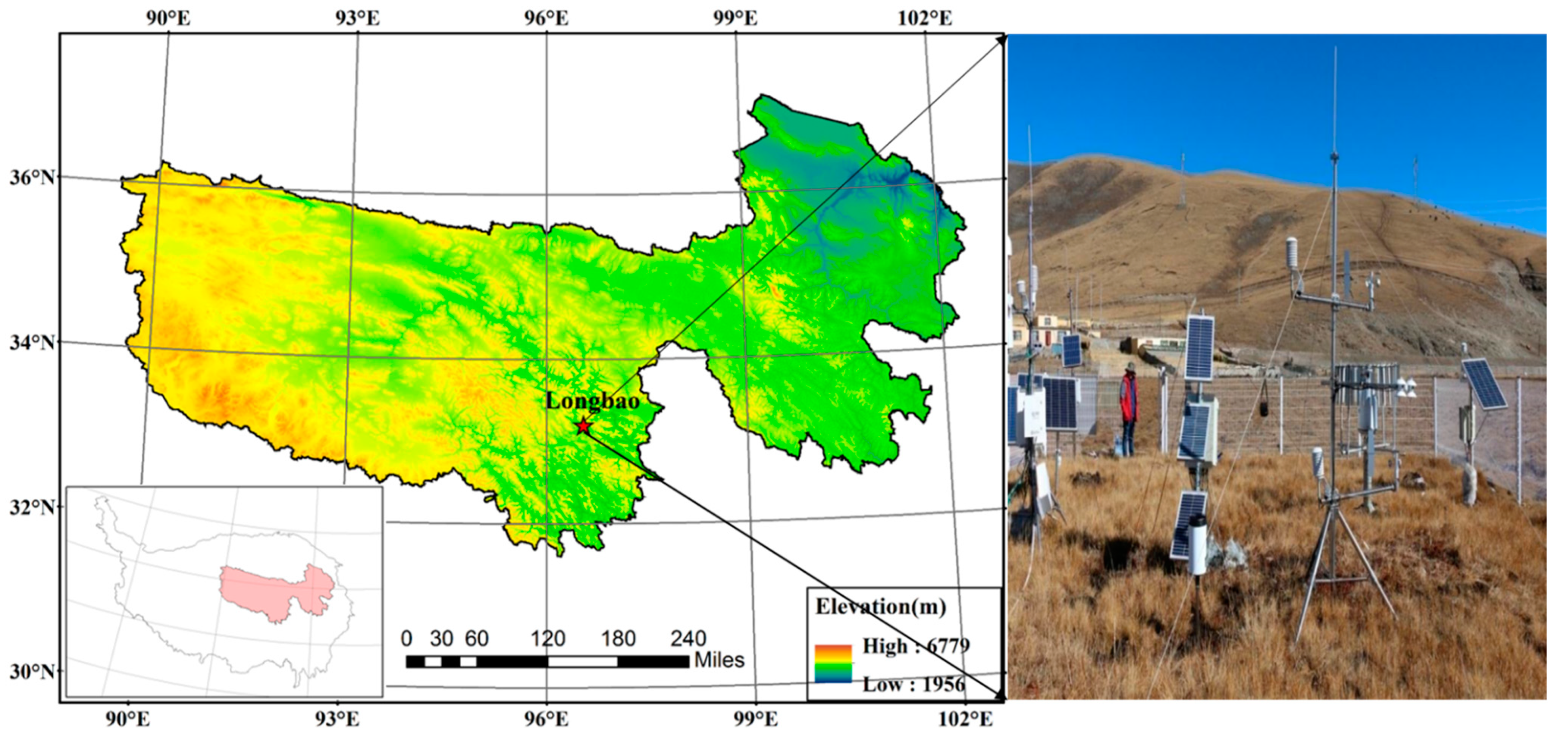
2.1. Sampling Site and Data Survey

The experimental site was located at the Longbao Experimental Station (Longbao Station for short) at the Qinghai China Meteorological Administration cold ecological meteorological field science experimental base (Figure 1). Longbao Station is located in the Longbao Wetland Nature Reserve, which is northwest of Yushu City, Yushu Prefecture, Qinghai Province, China. It is 4167 m above mean sea level and is located at 96.55° E, 33.2° N, with an annual mean temperature of −0.4°C and an annual precipitation of 731 mm [15]. The underlying vegetation type is typical alpine wetland. Kobresia Tibetica, K. pygmaea, and K. humilis are the main herbage species in the plot. Kobresia Tibetica accounts for 60–70% of forage species [15], and the soil type of the plot is mainly alpine marshland [15].

The Longbao Experimental Station was built in 2011, and its micrometeorological observation system was put into operation after the station was built in 2011. The vorticity flux observation equipment was built and put into operation in July 2018. A high observation tower of 2.5 m was set up at Longbao Station, and an open-circuit eddy correlation system (Li-7500A, Li-cor, Logan, Lincoln, NE, USA) was installed to measure three-dimensional wind speed and carbon dioxide and water vapor concentrations at 10 Hz. To process raw data collection, the half-hour mean value of NEE and evapotranspiration (ET) were calculated after removing peaks, two-dimensional coordinate rotation, time-lag compensation, and density fluctuation correction using open-source software Eddypro 6.0 [16,17]. The observation program also included micrometeorological forcings, including air pressure, four-component radiation (1.5 m), photosynthetic effective radiation (1.5 m), wind speed and wind direction of two layers (1 m/2 m), soil temperature and humidity of five layers (0.05/0.1/0.2/0.3/0.4 m), two soil heat fluxes (8 cm/10 cm), precipitation (0.75 m), and air temperature and humidity of two layers (1 m/2 m). The parameters of the power supply and data acquisition accessories were three 20 W solar panels, a 65 AH colloid cell, a CR1000 data acquisition device, and an AM16/32B Expansion Panel. The eddy correlation observation system was equipped with three 80 W solar panels, one 100 AH colloidal cell, and one 120 AH colloidal cell. The data were CR3000 and CR1000.

The data from Longbao Station were selected from the original data observed by the vorticity correlation system from January to October in 2019; data quality levels were chosen with QC = 0 and QC = 1 (QC of 0 indicates the highest data quality, 1 is average, and 2 is poor). The data missing from the NEE observations are shown in

Table 1. Statistical table showing the absence of observed NEE in the study area.

Station Name	Percentage of Level 0	Percentage of Level 1	Percentage of Level 2	Missing Rate
Longbao	47.22	24.26	10.60	17.92

, with a missing data rate of 17.92 percent in 2019. Among them, 47.22% were grade 0 quality data, 24.26% were grade 1 quality data, and 10.60% were grade 2 quality data.

2.2. Studying Methods

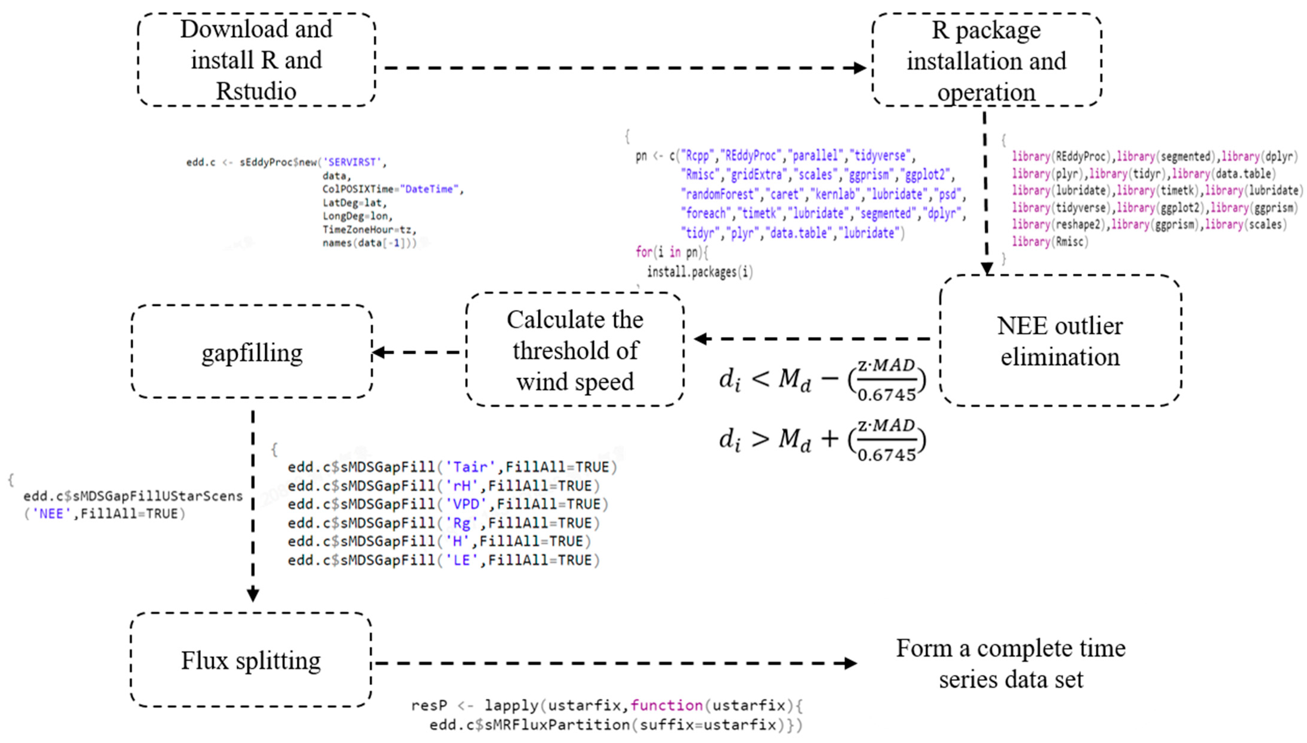
2.2.1. Reddyproc Algorithm

The Reddyproc algorithm first performed quality checks and filters based on the relationship between measured flux and friction velocity to discard biased data [2]. Second, we filled in data gaps based on information from environmental conditions [18]. Finally, the net flux of carbon dioxide was divided into its total flux into and out of the ecosystem through night-based and day-based methods [19]. The core algorithm included four points: First, median absolute deviation (MAD) was used to detect and eliminate the NEE outliers. Second, the night friction wind speed threshold was calculated. The frictional wind speed decreased, and the NEE measured with eddy correlation system was underestimated when the atmospheric turbulence was weak at night [20,21]. To avoid systematic bias in nighttime NEE data [2], it is usually necessary to determine the frictional wind velocity threshold, thereby excluding NEE below the frictional wind velocity threshold [22]. Third, NEE was interpolated. Filtered flux data with time series gaps and missing data need to be interpolated using existing flux data and meteorological measurements after filtering NEE data according to different seasonal friction wind speed thresholds. The interpolation step used three kinds of meteorological data, e.g., RG, Tair, and VPD. (1) If all three meteorological data were missing, lookup table (Lut) was used. (2) If Tair or VPD were missing, only RG was used. (3) If all three meteorological data were missing, mean diurnal course (MDC) was used. Finally, the flux was divided according to the relationship between total primary productivity (GPP), ecosystem respiration (Reco), and NEE (NEE = Reco − GPP) [18]. The nighttime NEE data splitting method assumes that Reco is only related to temperature change and that nighttime vegetation is only respirable. Therefore, the Reco change of daytime vegetation can be inferred from the response curve of nighttime NEE to temperature, and the GPP can be calculated according to the above relationship. The daytime NEE data splitting approach assumes the relationship between daytime NEE and total radiation to be a composite of the effect of RG and VPD on GPP and the effect of temperature on Reco [23,24]. These total fluxes are essential for understanding land–air interactions.

Lookup tables (LUT) were created for each site so that missing values of NEE could be looked up based on the environmental conditions associated with the missing data. Tables were created to represent changing environmental conditions based on either six bimonthly periods or four seasonal periods. In mean diurnal course (MDC), a missing observation was replaced by the mean for that time period (half hour) based on adjacent days. The methods for derivation of mean diurnal pattern of bin-averaged (half-) hourly measurements differed mainly in the length of the time interval of averaging (window size of usually 4–15 days) (Figure 2). R and Rstudio from https://cloud.r-project.org/ and https://www.rstudio.com/ (April 2020).

2.2.2. Machine Learning Algorithm

The interpolation effect of machine learning algorithm was studied using the effective meteorological factors of 30 min and NEE observations. The shortwave downward radiation, saturated water pressure, air temperature, relative humidity, soil temperature, soil heat flux, soil water content, and wind speed were measured with the micrometeorological observation system for 30 min from January to October 2019. Using them as input variables, the NEE observations of the corresponding time periods were taken as output variables. Additionally, 80% of the observations were taken as training sets, and 20% were taken as test sets for training. Machine learning regression algorithm was used to interpolate the missing or discarded data to obtain the complete flux time series, and multiple linear regression (MLR), classification regression tree (CART), random forest (RF), multilayer perceptron (MLP), K-nearest neighbor (KNN), adaptive boosting (ADABOOST), gradient boosting regression tree (GBRT), and extreme gradient boosting (XGBoost) were used in this study.

The purpose of MLR is to construct a linear model on the existing data set through two or more independent variables to fit the relationship between the components of the feature vector of the data set and to find a straight line or a hyperplane to minimize the error between the predicted value and the value [25,26]. CART is a tree structure where each internal node represents a test on an attribute, each branch represents a test output, and each leaf node represents a category. The decision tree adopts a top-down recursive method. The basic idea is to construct a tree with the fastest entropy decrease based on information entropy. The entropy at the leaf node is zero. At this time, the instances in each leaf node belong to the same class [25,26,27]. The essence of random forest (RF) is to randomly select k new self-help sample sets from the samples and to construct k classification regression trees. The samples that are not extracted each time form K out-of-bag data. Each tree grows to maximum without any cutting. The generated trees are composed of random forests, and the new data are classified by random forests. The classification results depend on the number of tree classifier votes [25,26,27]. Multilayer perceptron (MLP), also known as artificial neural network, first randomly initializes all parameters and then iteratively trains and continuously calculates the gradient and updates the parameters until a certain condition is satisfied (such as the error being small enough and the number of iterations being large enough); that is, it optimizes them [28,29,30,31]. K-nearest neighbor (KNN), given a training data set, for a new input instance, finds k instances nearest to the instance in the training set. The majority of these k instances belong to which class the instance belongs to. KNN includes three important elements: distance measurement, k-value selection, and classification decision rules. KNN distance measure generally uses the Euclidean distance measure [28,29,30,31]. Adaboost is a boosting algorithm that learns multiple weak classifiers by changing the weight of training samples and that linearly combines them into a strong learner. Firstly, the weight of the wrong samples classified by the weak classifier in the previous round is increased, and the weight of the correct samples is reduced. Secondly, the linear combination of multiple weak classifiers is carried out to improve the weight of weak classifiers with good classification effect and to reduce the weight of weak classifiers with high classification error rate [25,26,27]. The gradient boosting decision tree (GBRT) first gives an objective loss function whose domain is the set of all feasible weak functions (basis functions). Then, through iteration, a basis function in the negative gradient direction is selected to gradually approach the local minimum. This view of gradient boosting in the function domain has a profound impact on many areas of machine learning [25,26,27]. Extreme gradient boosting (XGBoost) is an efficient, flexible, and portable machine learning library implemented using the gradient boosting framework. It is a C++ implementation of GBRT. XGBoost still belongs to the GBDT algorithm in essence, but it is superior to the traditional GBDT algorithm in accuracy, speed, and generalization ability [31,32,33].

2.2.3. Model Evaluation Indicators

The goodness of fit (R²), root mean square error (RMSE), and mean absolute error (MAE) were used to evaluate the computational effectiveness of machine learning:

$$R^2={[{\sum }_{i=1}^n\left(x_i-\overline{x}\right)\left(y_i-\overline{y}\right)/\sqrt{{\sum }_{i=1}^n{\left(x_i-\overline{x}\right)}^2}\sqrt{{\sum }_{i=1}^n{\left(y_i-\overline{y}\right)}^2}]}^2$$

(1)

$$RMSE=\sqrt{\frac{1}{n}{\sum }_{i=1}^n{\left(x_i-y_i\right)}^2}$$

(2)

$$MAE=\frac{1}{n}{\sum }_{i=1}^n\left|x_i-y_i\right|$$

(3)

Among them, $x_i \mathrm{and} y_i$ are the measured values of NEE flux towers and the values of machine learning algorithms. $\overline{x} \mathrm{and} \overline{y}$ are the arithmetic mean values, and N is the number of data volumes. R² is the goodness of fit; it reflects the influence proportion of input factor on NEE. The closer the value is to 1, the greater the percentage change in NEE caused by input factor is. RMSE is the arithmetic square root of mean square error, which is used to measure the deviation of NEE prediction from the measured value. MAE is the average absolute error, which reflects the absolute magnitude of the NEE prediction error. This study used the sklearn module of Python to implement machine learning model training and the matplotlib module to implement all chart generations.

3. Results

3.1. Reddyproc Interpolation

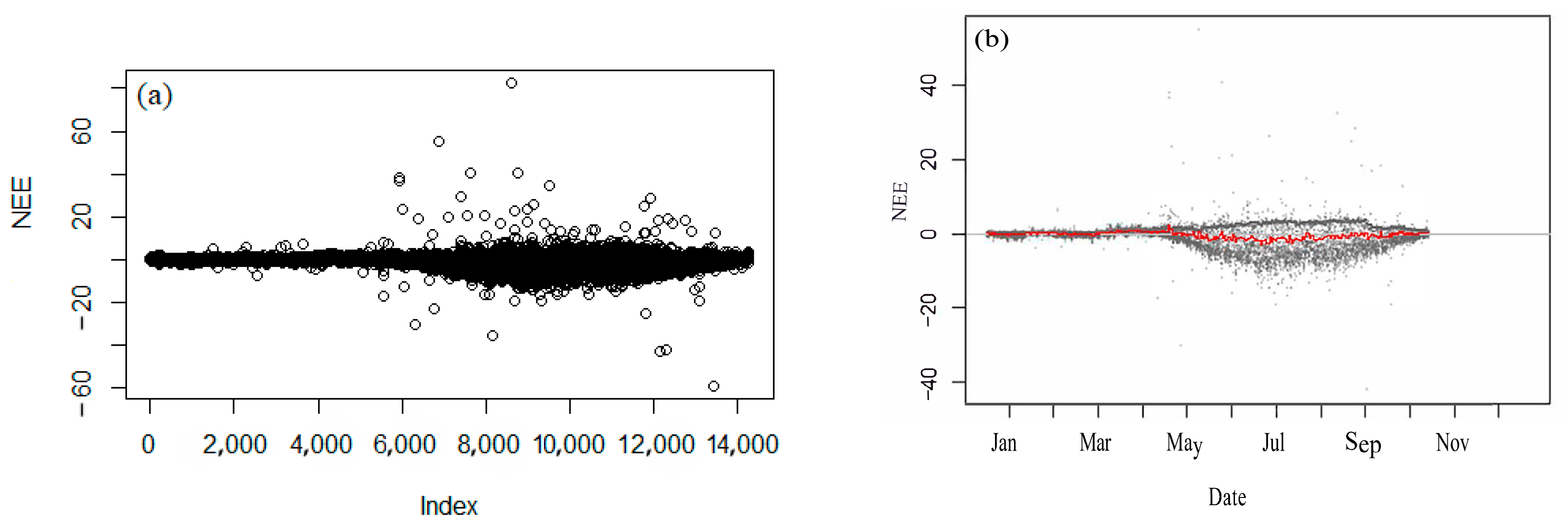
3.1.1. NEE Outlier Detection and Elimination

The criterion for judging the abnormality of the NEE observations was that the night friction velocity met the threshold condition; the critical value of friction velocity depended on the distribution trend of the NEE with friction velocity, the amount of high-quality data, the threshold value of the carbon flux, and rainfall. After these outliers were eliminated, the missing data were interpolated [34]. The outlier detection algorithm was used to detect the peak value according to the position of each half-hour value relative to the before and after half-hour values; according to daytime, total radiation (RG), and heat sensitivity (h), the daytime and nighttime values were divided into two groups. In this study, DR > 10 W M⁻² or H > −4.3 W M⁻² was set as the daytime values, and DR ≤ 10 W M⁻² or, alternatively, H ≤ −4.3 W M⁻² was set as the nighttime values. The window in which each sample was located was set to 13 days [2], and di was calculated according to Formula (4). Then, the median di in each window, day and night, was calculated separately to obtain Md. Finally, according to Formula (7) and Formula (8), the number of outliers eliminated was 346, accounting for 3% of the valid data.

$$d_i=\left(NE{E}_i-NE{E}_{i-1}\right)-\left(NE{E}_{i+1}-NE{E}_i\right)$$

(4)

$$M_d=\left(d_i-d_{i-1}\right)-\left(d_{i+1}-d_i\right)$$

(5)

$$MAD=median\left(\left|d_i-M_d\right|\right)$$

(6)

$$d_i<M_d-\left(\frac{z·MAD}{0.6745}\right)$$

(7)

$$d_i>M_d+\left(\frac{z·MAD}{0.6745}\right)$$

(8)

3.1.2. Interpolation Precision

The determination coefficient (R²), root mean square error (RMSE), and absolute mean error (MAE) were used to evaluate the interpolation accuracy of the Reddyproc algorithm. The determination coefficient of the CO₂ flux fitting obtained through the Reddyproc algorithm was 0.65 (

Table 2. Interpolation accuracy of Reddyproc algorithm.

Station Name	Pearson	R2	RMSE	MAE
Longbao	0.80	0.65	1.91	1.34

Pearson represents Pearson correlation coefficient, R² represents coefficient of determination, RMSE represents root mean square error, and MAE represents mean absolute error.

). In addition, before the Reddyproc algorithm interpolated the missing values, it was necessary to detect the occasional spikes, namely, the outliers, in the half-hour flux data through the outlier detection technique, which usually does not directly affect the annual NEE. However, it affects the quality of the populated data set. Figure 3 shows the CO₂ flux data with the outliers not eliminated on the left, and there are obvious discrete values in some time periods with large deviations. Meanwhile, on the right, the outliers shown were detected and eliminated based on the outlier detection algorithm. After removing outliers, the quality of the CO₂ flux data was improved, and the dispersion was decreased, which indicated that the interpolation data was of a high precision and reliable quality.

3.2. Machine Learning Interpolation

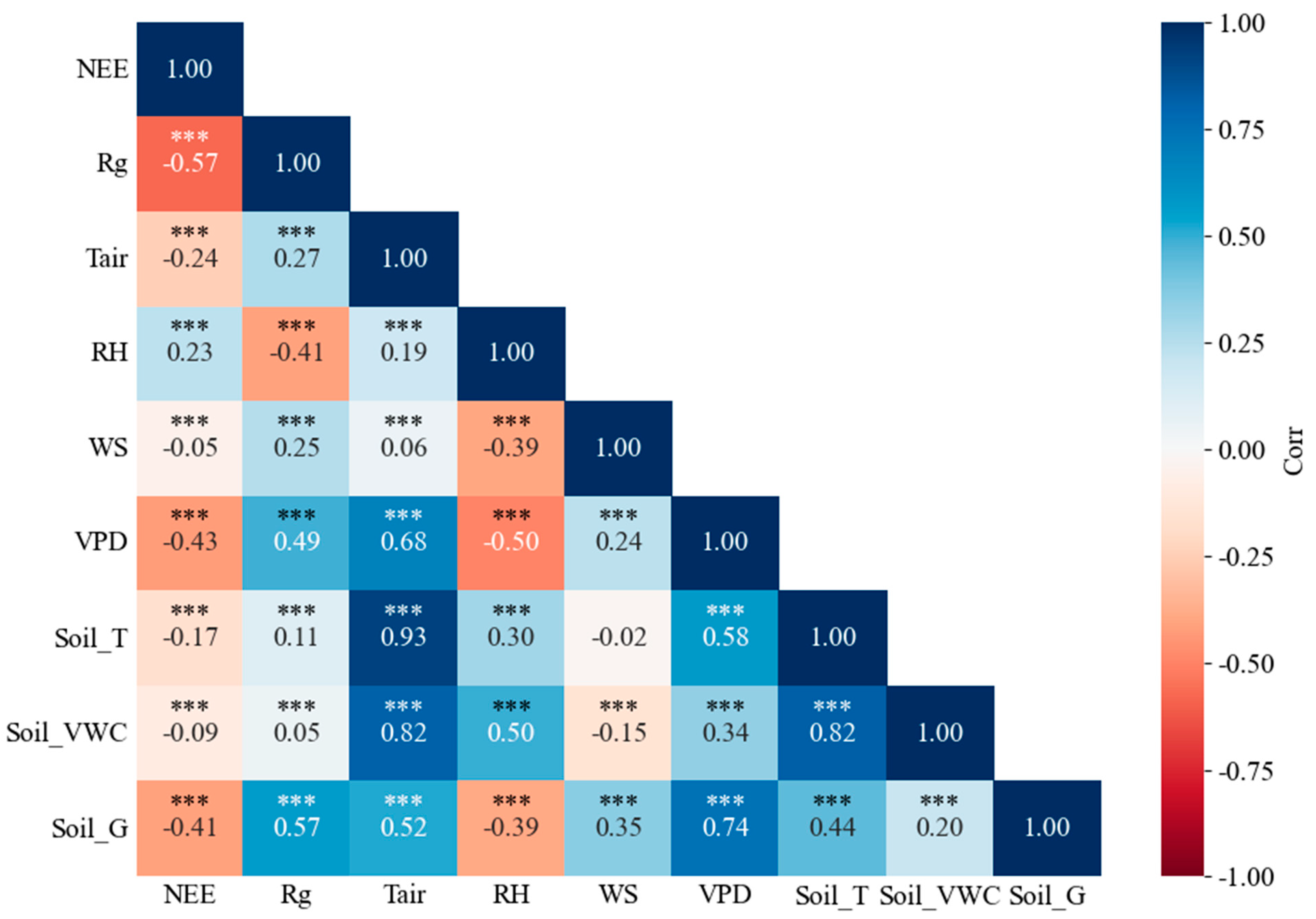
3.2.1. Correlation Analysis between NEE and Meteorological Factors

The amount of a CO₂ flux is affected by the climate, the land type, the vegetation status, and other factors. In order to explore the sensitivity of the CO₂ flux to environmental factors, we selected meteorological factors for CO₂ flux interpolation, and the 30 min data of the input meteorological factors and the CO₂ flux were selected for the correlation analysis. The Pearson correlation coefficient in statistics was used to measure the linear correlation between the CO₂ flux and the meteorological factors in this paper. The results show that there was a significant correlation between the CO₂ flux and the selected meteorological factors in the study area, and the significant p values were less than 0.001, indicating that the level was significant. The correlation was as follows: shortwave downward radiation (RG) > saturated water vapor pressure (VPD) > soil heat flux (Soil_G) > air temperature (Tair) > relative humidity (RH) > soil temperature (Soil_T) > soil moisture content (Soil_VWC) > wind speed (WS). The CO₂ flux was negatively correlated with RG, VPD, Soil_G, Tair, Soil_T, Soil_VWC, and WS, and it was positively correlated with RH as shown in Figure 4.

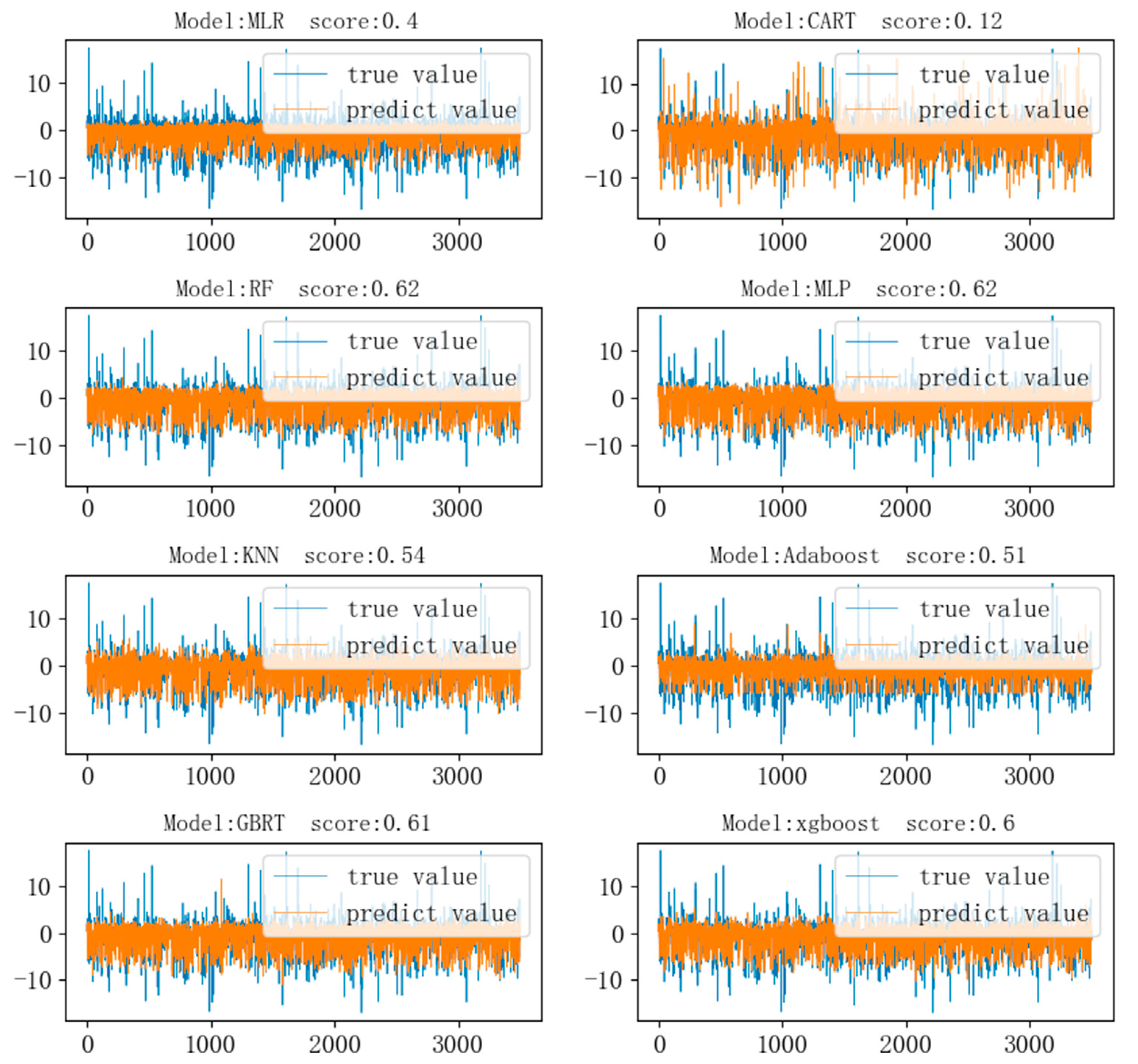
3.2.2. The Accuracy Comparison of Each Model Algorithm under Different Meteorological Factor Input Combinations

According to the correlation analysis between the NEE and the meteorological factors in Figure 4, the first three meteorological factors of the average correlation coefficient were selected as the characteristic combination 1. Moreover, the range from combination 2 to combination 6 was added according to the order of the average correlation coefficients, and six input combinations based on the machine learning algorithm were built. A total of 80% of the observed values were used as the training set, and 20% were used as the test set (

Table 3. Model parameter combinations of different meteorological factors.

Feature Combination	Input Characteristics	Feature Number
combination 1	RG, VPD, Soil_G	3
combination 2	RG, VPD, Soil_G, Tair	4
combination 3	RG, VPD, Soil_G, Tair, RH	5
combination 4	RG, VPD, Soil_G, Tair, RH, Soil_T	6
combination 5	RG, VPD, Soil_G, Tair, RH, Soil_T, Soil_VWC	7
combination 6	RG, VPD, Soil_G, Tair, RH, Soil_T, Soil_VWC, WS	8

).

It can be seen from

Table 4. Model accuracy under different combinations of meteorological factors.

Feature combination	MLR			CART			RF			MLP
	R2	RMSE	MAE	R2	RMSE	MAE	R2	RMSE	MAE	R2	RMSE	MAE
combination 1	0.32	2.60	1.65	0.22	2.99	1.64	0.58	2.19	1.16	0.57	2.17	1.11
combination 2	0.36	2.54	1.57	0.24	2.93	1.64	0.60	2.17	1.14	0.60	2.10	1.14
combination 3	0.36	2.54	1.57	0.25	2.87	1.57	0.60	2.22	1.21	0.61	2.10	1.14
combination 4	0.36	2.54	1.57	0.22	3.03	1.57	0.59	2.17	1.15	0.61	2.11	1.14
combination 5	0.36	2.53	1.57	0.22	2.98	1.51	0.60	2.15	1.10	0.61	2.10	1.14
combination 6	0.38	2.51	1.55	0.25	2.86	1.46	0.62	2.10	1.08	0.62	2.18	1.12
Average	0.36	2.54	1.58	0.23	2.94	1.57	0.60	2.17	1.14	0.61	2.13	1.13
Feature combination	KNN			Adaboost			GBRT			XGBoost
	R2	RMSE	MAE	R2	RMSE	MAE	R2	RMSE	MAE	R2	RMSE	MAE
combination 1	0.52	2.16	1.35	0.40	2.29	1.24	0.56	2.20	1.17	0.58	2.17	1.11
combination 2	0.54	2.14	1.37	0.42	2.33	1.24	0.59	2.19	1.12	0.59	2.19	1.54
combination 3	0.54	2.24	1.37	0.44	2.27	1.27	0.56	2.22	1.15	0.61	2.19	1.54
combination 4	0.52	2.24	1.37	0.44	2.29	1.27	0.57	2.20	1.15	0.61	2.11	1.54
combination 5	0.56	2.23	1.41	0.42	2.28	1.21	0.57	2.19	1.10	0.60	2.10	1.54
combination 6	0.56	2.21	1.40	0.46	2.28	1.26	0.59	2.20	1.10	0.62	2.10	1.52

that, in combination 1, MLR, CART, and Adaboost had poor prediction effects, and the accuracy R² was less than 0.5. RF and XGBoost had the highest prediction accuracies, and R² reached 0.58. In combination 2, CART had the lowest prediction accuracy (R² = 0.24), and RF and MLP had the highest prediction accuracies (R² = 0.60). In combination 3, CART had the lowest prediction accuracy (R² = 0.25), and MLP and XGBoost had the highest prediction accuracies (R² = 0.61). In combination 4, CART had the lowest prediction accuracy (R² = 0.22), and MLP and XGBoost had the highest prediction accuracies (R² = 0.61). In combination 5, CART had the lowest prediction accuracy (R² = 0.22), and MLP had the highest prediction accuracy (R² = 0.61). In combination 6, CART had the lowest prediction accuracy (R² = 0.25), and RF, MLP, and XGBoost had the highest prediction accuracies (R² = 0.62).

The R² values of the eight types of machine learning algorithm models in combination 6 were the largest among the six feature combinations, which showed that the feature factor of combination 6 was the best input for the model training. Figure 5 shows the prediction accuracies in combination 6 among the eight machine learning models.

From Table 4 and Figure 4, it can be concluded that the change rate of RMSE in the eight algorithms ranged from 2% to 6%, which included 4% for MLR, 6% for CART, 6% for RF, 2% for MLP, 4% for KNN, 3% for Adaboost, 3% for GBRT, and 4% for XGBoost. Under the six combinations, the R² of the MLP model was between 0.60 and 0.62, the RMSE was between 2.10 and 2.18, and the MAE was between 1.11 and 1.14. Under the combination of the different meteorological factors, the average of R² was the best, the RMSE change rate was the lowest, and the stability was the best.

3.3. Comparison of Reddyproc and MLP Interpolation Effect

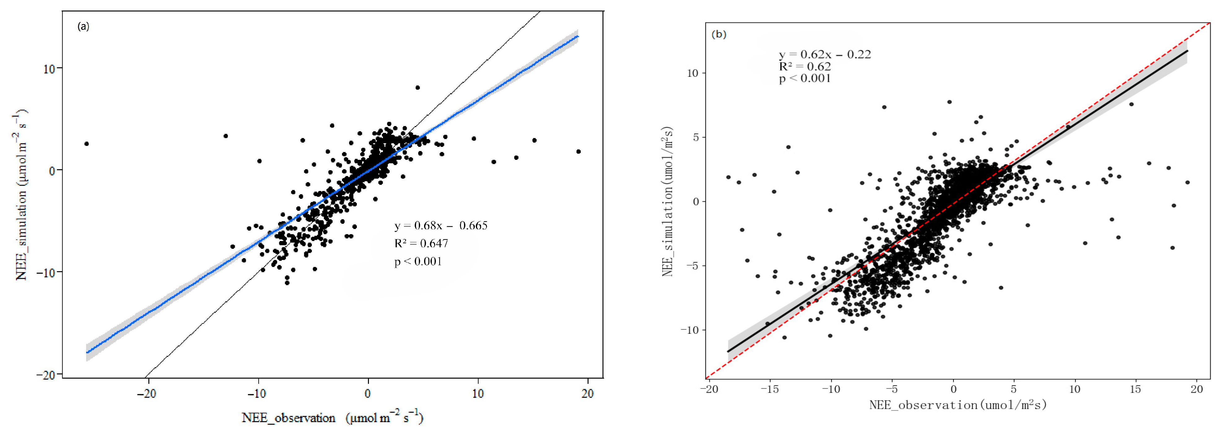
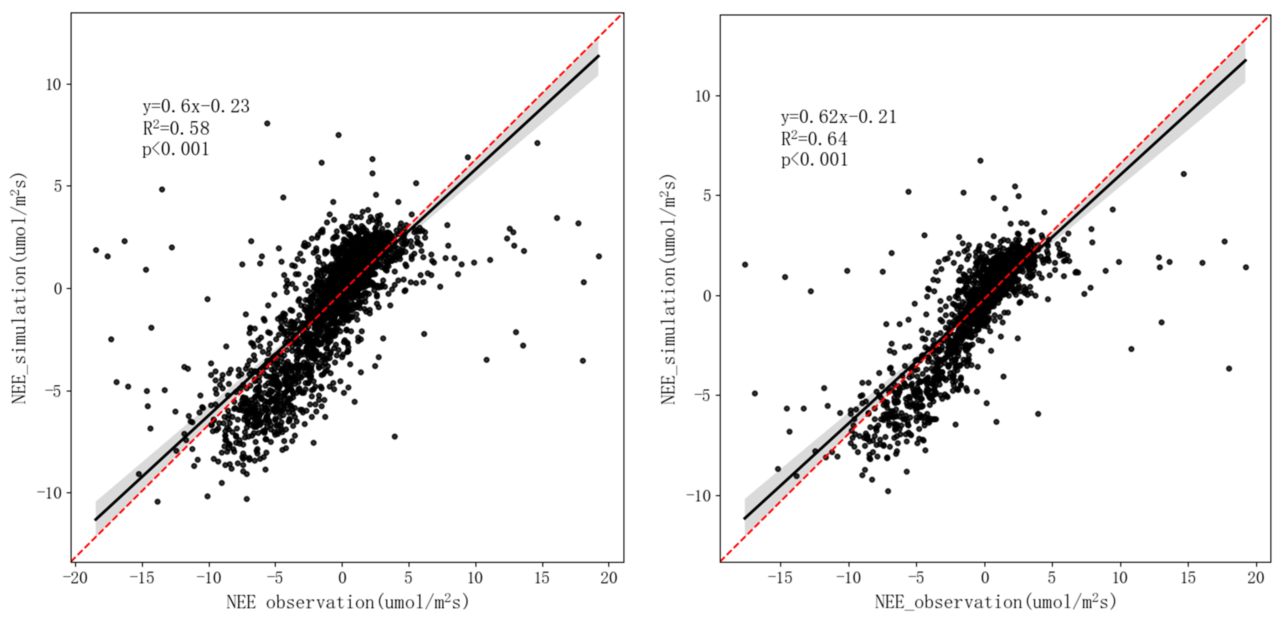
3.3.1. Interpolation Precision

Figure 6 shows the decision coefficients R² of the Reddyproc and MLP algorithms for the CO₂ flux fitting. The decision coefficient of the Reddyproc estimation model was larger than that of the MLP estimation model, and the noise influence of the MLP model was larger than that of Reddyproc.

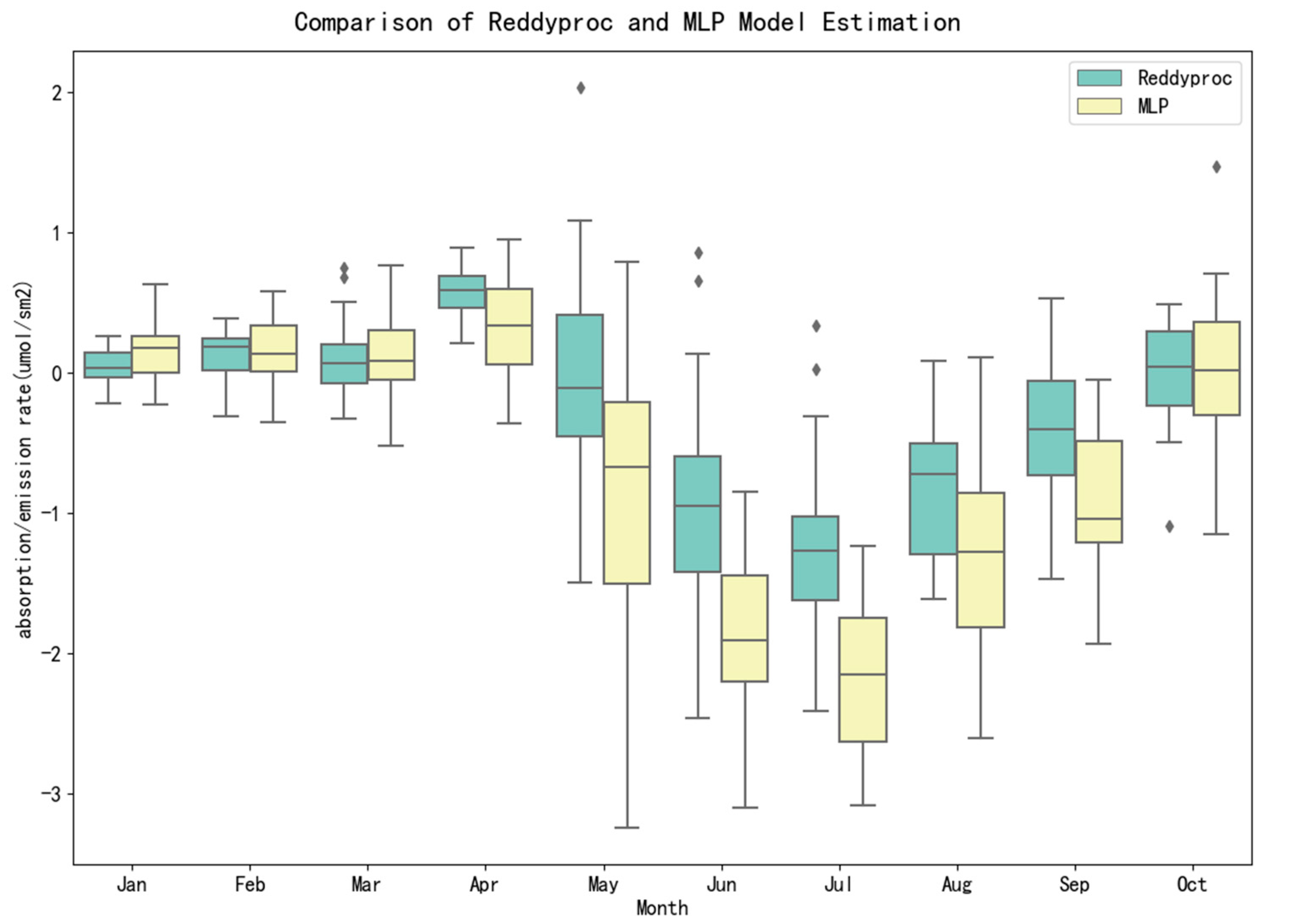
3.3.2. Monthly Scale NEE Variation Characteristics

The Reddyproc and MLP models estimated the monthly change in the NEE at the Longbao Station, which is shown in Figure 7. The filling effect of missing data had almost the same effect on the whole-year data. The net absorption reached its maximum in July, which was −1.26 μmol S⁻¹ M⁻². The emission rate reached its maximum in April, which was 0.57 μmol S⁻¹ M⁻². With the development of the vegetation structure, the carbon absorption increased, and it reached its maximum in the middle of the growing season. The results showed that the estimated value of Reddyproc was about 1.5 times lower than that of MLP in January, February, March, and October. However, from April to September, the monthly average of the former was higher than that of the latter by about 1.5–2 times. These results indicated that the machine learning algorithm tended to predict the carbon source more in the cold season (nongrowing season), and carbon sequestration was more likely to be predicted in the warm season (growing season).

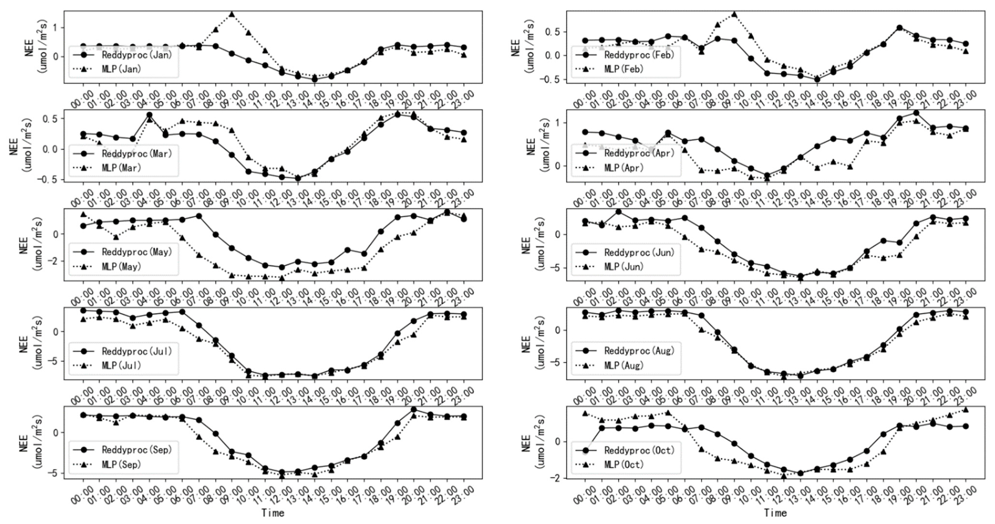
3.3.3. Hourly Scale NEE Variation Characteristics

The hourly variation in the NEE at the Longbao Station estimated with the MLP model is shown in Figure 8, and the monthly hourly absorption peaks at the Longbao Station were 14:00 in January, 14:00 in February, 13:00 in March, 11:00 in April, 12:00 in May, 13:00 in June, 11:00 in July, 12:00 in August, 12:00 in September, and 12:00 in October. The overall peak occurred between 11:00 and 14:00; the emissions peaked in January at 09:00, February at 09:00, March at 19:00, April at 20:00, May at 22:00, June at 21:00, July at 21:00, August at 22:00, September at 00:00, and October at 23:00, and the overall peak occurred between 21:00 and 00:00. The hourly variation in the NEE at the Longbao Station estimated with the Reddyproc model is shown in Figure 4. It was found that the peak of absorption estimated with REDDYPROC was 1–2 h later than that estimated with the MLP model in July and August. The peaks at the other time periods were similar, which was consistent with the above finding that MLP was estimated to be higher in the warm season (growing season) than in Reddyproc. As a result, the absorption rate of the NEE reached its peak faster in the MLP model.

4. Discussion

4.1. Input Factor Selection in the Model

It can be seen from Section 3.2.2 that the R2 variation range of the eight types of machine learning algorithm models in the six combinations was 0.22–0.62, the RMSE variation range was 2.10–2.99, and the MAE variation range was 1.08–1.65. The input factors in combination 1 were the top three meteorological factors (RG, VPD, Soil_G), which were ranked by the correlation coefficients in Figure 4. When the temperature was added, the prediction accuracy of the eight models was improved, and the R² increased by 2~13%, which is consistent with the conclusion obtained by Wang Sheng et al. [35] when using machine learning to fit water flux; that is, the accuracy of the models obtained by each algorithm increases with an increase in the number of input features. Then, the meteorological factors RH, Soil_T, Soil_VWC, and WS were added to the model input factors in turn. The results showed that, when RH, Soil_T, and Soil_VWC were added, the prediction accuracies of MLR, RF, and MLP were almost unchanged and that the prediction accuracies of KNN, Adaboost, GBRT, and XGBoost fluctuated obviously. In terms of stability, MLP was the highest, and CART and RF were the worst, which is the same as the research results of Mao et al. [36] and Hassan et al. [37]. In other words, the RF algorithm had a serious overfitting phenomenon because the tree model had a high dependence on the continuity of the data distribution, and the RF model was easy to fall into overfitting in some sample sets with large noise. After adding WS, the R² of the eight models increased significantly. The Pearson correlation coefficient between the CO₂ flux and WS was zero, and the significant p value was less than 0.001, indicating that WS was also a key factor affecting the CO₂ flux in the Longbao area. This conclusion shows that the determination of the input factors in the algorithm model was not completely consistent with the correlation conclusion. The selection of the input factors needed to be added one by one on the basis of the correlation analysis to obtain the best model feature combination.

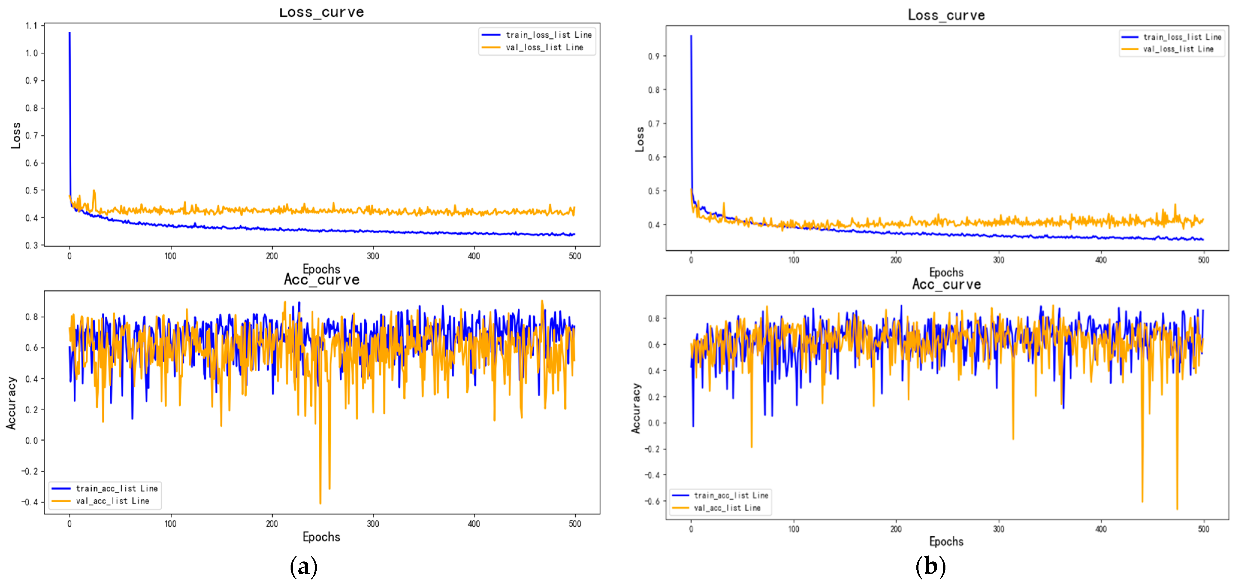
4.2. Improved MLP Deep Learning Model

The Reddyproc model could obtain a better NEE estimation model with fewer input parameters, while the machine learning prediction model had eight input features. However, in the high-latitude and high-altitude area, the above-mentioned machine learning models were greatly limited in the study of ecosystem carbon assessment in the absence of corresponding measured data due to the limited observation elements, the harsh climate conditions, and the uneven distribution of the observation sites. Is it possible to find a model that does not require the relevant physical parameters of the high-cold region, greatly reducing the parameters of the model, and would it be more suitable than conventional machine learning models for regions that are without or lacking data? Huang et al. (2021) [38] applied an artificial neural network to a frozen soil hydrological model of small watersheds in the hinterland of the Qinghai–Tibet Plateau. After training, the model could simulate and predict the runoff in a small watershed in the frozen soil area of the Qinghai–Tibet Plateau by relying on precipitation and temperature as inputs. It provided a simple and effective method with a certain physical significance for the study of the runoff of small watersheds in a frozen soil area without observation data, such as soil temperature and moisture. Peng et al. (2018) [39] applied the BP neural network algorithm to the estimation of water flux and found that the performance of the neural network model was significantly better than that of the machine learning model under the same conditions, which indicated that they have strong adaptability. Y. Lecun (2015) [40] further elucidated the deep learning algorithm, which differs from machine learning in that the traditional machine learning framework is feature extraction and classification, while the deep learning framework is feature learning and classification, and the latter has a stronger learning ability and generalization ability.

In this study, the MLP model was found to be the most stable, with input characteristics ranging from three to eight variables, and the fitting accuracy fluctuated by about 1%. Considering that the MLP model was stable and optimal, the MLP deep neural network was used for NEE prediction. Additionally, the multilayer perceptron was based on the single layer neural network, which was composed of one or more hidden layers, and, thus, became the deep neural network. Its parameters were adjusted through supervised learning and forward and backward propagation, which accorded with the Y. Lecun (2015) [40] analytic deep learning framework. The network input dimension was set to have five parameters, referring to the five meteorological factors in Section 2.2.1, which had a relatively high correlation between the NEE and meteorological factors, including shortwave downward radiation (RG), saturated water pressure (VPD), air temperature (Tair), relative humidity (RH), and wind speed (WS). The learning rate of multilayer perceptron training was set to 0.001 through cross-validation and parameter tuning, and the batch size was set to 32. The training time epoch was set to 500, and the optimizer selected was Adam. Additionally, the hidden layer was set to 20,20,5. The output dimension was set to one, which was the NEE prediction value. The model decision coefficient R² obtained through the training of this network model was 0.58, which was larger than that of the previous MLP model (0.57). It showed that the precision of the deep learning model can be improved by using fewer input parameters under the optimization of the network structure, and this compares with Deng Mengjiao (2022) [41] and Xia Guoen (2020) [42], who quantitatively evaluated and compared the multilayer perceptron of the algorithms with CART, KNN, NB, RF, and SVM by using accuracy and F1 (a comprehensive evaluation of precision and recall). Additionally, compared with the performance of the algorithms with those of CART, K-nearest neighbor (KNN), Naïve Bayes (NB), RF, and SVM, the accuracy of the multilayer perceptron method was consistent with the results of the study with the highest F1 score, further indicating that the deep learning model has a stronger learning ability and generalization ability.

4.3. Timing Anomaly Detection

The depth model of MLP had a good learning ability and prediction accuracy with five input features, but the estimation ability of the NEE was still lower than that of the Reddyproc model on the whole. Considering that the Reddyproc algorithm includes outlier detection technology as can be seen from Figure 3, the outlier detection algorithm based on the NEE data outlier detection and elimination of the data dispersion was reduced, and the data quality was improved. Papale et al. (2006) [2] performed quality checks and filtering based on the relationship between the measured flux and friction velocity, using the absolute bias median of the outlier estimator (MAD) for outlier detection on the basis of a double-difference time series, to discard biased data. The problem of anomaly detection has been widely studied in various fields and applications. Chandola et al. (2009) [43] and Toledano et al. (2017) [44] pointed out that anomaly detection aims at finding unusual data values or patterns in time series data that do not satisfy the normal constraint rules of a given model, and, in many practical applications, it has certain practical value.

In order to explore the importance of time series anomaly detection in NEE model prediction, the training was carried out after the time series anomaly value of the NEE was eliminated. The outliers here were timestamp values where the observed NEE was different from the expected NEE of the time series. When a particular time instant was compared with the other values in the time series (global outliers) or with its neighbors (local outliers), it presented an anomaly. IOR was used to set the threshold and to judge the outliers by the threshold. The red color indicated the outliers. Figure 9 shows the training curve of the MLP training model before and after NEE timing anomaly detection; the accuracy curve of the MLP prediction model in the test set was lower than that in the training set, which showed that the model did not perform well in the test set, and the model determination coefficient R² was 0.58. The prediction accuracy of the MLP prediction model in the test set was better, and the model determination coefficient R² was raised to 0.64 (Figure 10), which showed that the elimination of the time series outliers had a great influence on NEE simulation. Stable laminae, which were often present at night, inhibited turbulence, leading to an underestimation of the nocturnal NEE, that is, ecosystem respiration (Van Gorsel et al., 2007) [45], as Massman and Lee (2002) [46] suggested. Specifically, adverse conditions could be detected by examining the relationship between the nocturnal NEE and u*, and Reddyproc provided this method, which allowed the determination of the nighttime friction wind velocity thresholds under conditions that were not considered as such [42,43]. The nighttime flux could be estimated accurately. Machine learning (ML) and deep learning (deep learning) lacked the understanding of the mechanism between the variables; however the data parameters were required to be low, so they were not as good as Reddyproc in the estimation of the NEE. The results further showed that the understanding of the underlying mechanism of the NEE was of great significance to the prediction model.

5. Conclusions

This study compares two filling methods, i.e., machine learning and Reddyproc, with respect to estimating the carbon flux through the eddy covariance data measured in the high-latitude Qinghai–Tibet plateau area, which showed a good approximation of the original data in the case that the amount of the data to be filled was small. In general, the Reddyproc model obtained better NEE estimates with fewer input parameters, which outperformed the machine learning model.

The accuracy of the gap filling method depends on the preprocessing of the data used to parameterize the filling algorithm, particularly when determining the friction wind speed threshold for the nighttime data. In this case, we should strongly emphasize that restudying the “nighttime” problem, in theory and through experiments, is the prerequisite for processing eddy covariance data. We believe that the detection and elimination of NEE time series anomalies were very important for the subsequent model training and prediction, and the precision was significantly improved, which showed that the outlier detection technology had a great influence on the simulated NEE. In addition, we found that the estimated values of the Reddyproc model and the MLP model had obvious seasonal differences. The MLP prediction was about 1.5 times higher in the cold season (nongrowing season) and about 2 times lower in the warm season (growing season).

This work contributes to the efforts of the flux community, collecting continuous measurements of the ecosystem carbon and energy exchange, by compiling consistent, quality assured, and documented datasets from a variety of worldwide ecosystems. The standardization of the data postprocessing assured justified comparable data to address intercomparisons across natural and managed ecosystems, climatic gradients, and multiple years and to investigate the processes controlling the carbon and energy fluxes of these systems.

References

1. Wang, S.; Zhang, Y.; Meng, X.; Song, M.; Shang, L.; Su, Y.; Li, Z. Fill the Gaps of Eddy Covariance Fluxes Using Machine Learning Algorithms. Plateau Meteorol. 2020, 39, 1348–1360. [Google Scholar]
2. Papale, D.; Reichstein, M.; Aubinet, M.; Canfora, E.; Bernhofer, C.; Kutsch, W.; Longdoz, B.; Rambal, S.; Valentini, R.; Vesala, T.; et al. Towards a standardized processing of Net Ecosystem Exchange measured with eddy covariance technique: Algorithms and uncertainty estimation. Biogeosciences 2006, 3, 571–583. [Google Scholar] [CrossRef] [Green Version]
3. Mauder, M.; Foken, T.; Clement, R.; Elbers, J.A.; Eugster, W.; Grünwald, T.; Heusinkveld, B.; Kolle, O. Quality control of CarboEurope flux data-Part 2: Inter-comparison of eddy- covariance software. Biogeosciences 2008, 5, 451–462. [Google Scholar] [CrossRef] [Green Version]
4. Xu, Z.; Liu, S.; Gong, L.; Wang, J.; Li, X. A Study on the Data Processing and Quality Assessment of the Eddy Covariance System. Advancesinearthscience 2008, 23, 357–370. [Google Scholar]
5. Wang, S.; Zhang, Y.; Lv, S.; Ao, Y.; Li, S.; Cheng, S. The Preliminary Study on Turbulence Data Quality Control of Jinta Oasis. Plateau Meteorol. 2009, 28, 1260–1273. [Google Scholar]
6. Lu, S.; Wen, J.; Zhang, Y.; Wang, S.; Zhang, T.; Tian, H.; Liu, R. Influence of the Different Averaging Period on Computing the Turbulent Fluxes Using LOPEX10 Data. Plateau Meteorol. 2012, 31, 1530–1538. [Google Scholar]
7. Zhuang, J.; Wang, W.; Wang, J. Flux Calculation of Eddy-Covariance Method and Comparison of Three Main Softwares. Plateau Meteorol. 2013, 32, 78–87. [Google Scholar]
8. Xu, X.; Zhou, G.; Du, H.; Shi, Y.; Zhou, Y. Effects of Interpolation and Window Sizes in Phyllostachys edulis forest for Parameter Estimation on Calculation of CO2 Flux. Sci. Silvae Sin. 2015, 51, 141–149. [Google Scholar]
9. Pastorello, G.; Trotta, C.; Canfora, E.; Chu, H.; Christianson, D.; Cheah, Y.W.; Poindexter, C.; Chen, J.; Elbashandy, A.; Humphrey, M.; et al. The FLUXNET2015 dataset and the ONEFlux processing pipeline for eddy covariance data. Sci. Data 2020, 7, 225. [Google Scholar] [CrossRef]
10. Beringer, J.; McHugh, I.; Hutley, L.B.; Isaac, P.; Kljun, N. Technical note:Dynamic integrated gap-filling and partitioning for OzFlux (DINGO). Biogeosciences 2017, 14, 1457–1460. [Google Scholar] [CrossRef] [Green Version]
11. Agarwal, D.; Pastorello, G.; Poindexter, C.; Papale, D.; Trotta, C.; Ribeca, A.; Canfora, E.; Faybishenko, B.; Samak, T. The data postprocessing pipeline for AmeriFlux data products. In Proceedings of the AGU Fall Meeting, New Orleans, LA, USA, 11–15 December 2017. [Google Scholar]
12. Moffat, A.M.; Papale, D.; Reichstein, M.; Hollinger, D.Y.; Richardson, A.D.; Barr, A.G.; Beckstein, C.; Braswell, B.H.; Churkina, G.; Desai, A.R.; et al. Comprehensive comparison of gap-filling techniques for eddy covariance net carbon fluxes. Agric. For. Meteorol. 2007, 147, 209–232. [Google Scholar] [CrossRef]
13. Dou, X. Applications of Machine Learning Methods in Modeling Carbon and Water Fluxes of Terrestrial Ecosystems; Xuzhou, China, 2018; pp. 1–145. [Google Scholar]
14. Zhu, X. Estimation of Ecosystem Respiration in the Grasslands of Northern China Using Deep Learning; Chongqing, China, 2020; pp. 1–101. [Google Scholar]
15. Quan, C.; Zhou, B.; Han, Y.; Zhao, T.; Xiao, J. A study of evapotranspiration on the degraded alpine wetland surface in the Yangtze River source area. J. Glaciol. Geocryol. 2016, 38, 1249–1257. [Google Scholar] [CrossRef]
16. Webb, E.K.; Pearman, G.I.; Leuning, R. Correction of flux measurements for density effects due to heat and water vapour transfer. Q. J. R. Meteorol. Soc. 1980, 106, 85–100. [Google Scholar] [CrossRef]
17. Li, H.Q.; Wang, C.Y.; Zhang, F.W.; He, Y.T.; Shi, P.L.; Guo, X.W.; Wang, J.B.; Zhang, L.M.; Li, Y.N.; Cao, G.M.; et al. Atmospheric water vapor and soil moisture jointly determine the spatiotemporal variations of CO2 fluxes and evapotranspiration across the Qinghai-Tibetan Plateau grasslands. Sci. Total Environ. 2021, 791, 148379. [Google Scholar] [CrossRef]
18. Reichstein, M.; Falge, E.; Baldocchi, D.; Papale, D.; Aubinet, M.; Berbigier, P.; Bernhofer, C.; Buchmann, N.; Gilmanov, T.; Granier, A.; et al. On the separation of net ecosystem exchange into assimilation and ecosystem respiration: Review and improved algorithm. Glob. Change Biol. 2005, 11, 1424–1439. [Google Scholar] [CrossRef]
19. Lasslop, G.; Reichstein, M.; Papale, D.; Richardson, A.D.; Arneth, A.; Barr, A.; Stoy, P.; Wohlfahrt, G. Separation of net ecosystem exchange into assimilation and respiration using a light response curve approach: Critical issues and global evaluation. Glob. Change Biol. 2010, 16, 187–208. [Google Scholar] [CrossRef] [Green Version]
20. Wutzler, T.; Lucas-Moffat, A.; Migliavacca, M.; Knauer, J.; Sickel, K.; Šigut, L.; Menzer, O.; Reichstein, M. Basic and extensible post-processing of eddy covariance flux data with REddyProc. Biogeosciences 2018, 15, 5015–5030. [Google Scholar] [CrossRef] [Green Version]
21. Desai, A.R.; Richardson, A.D.; Moffat, A.M.; Kattge, J.; Hollinger, D.Y.; Barr, A.; Falge, E.; Noormets, A.; Papale, D.; Reichstein, M.; et al. Cross-site evaluation of eddy covariance GPP and RE decomposition techniques. Agric. For. Meteorol. 2008, 148, 821–838. [Google Scholar] [CrossRef]
22. Aubinet, M.; Vesala, T.; Papale, D. Eddy Covariance; Springer: Dordrecht, The Netherlands, 2012. [Google Scholar]
23. Liu, M.; He, H.; Yu, G.; Sun, X.; Zhu, X.; Zhang, L.; Zhao, X.; Wang, H.; Shi, P.; Han, S. Impacts of uncertainty in data processing on estimation of CO2 flux components. Chin. J. Appl. Ecol. 2010, 21, 2389–2396. [Google Scholar]
24. Huang, K.; Wang, S.; Wang, H.; Yi, C.; Zhou, L.; Liu, Y.; Shi, H. An analysis of carbon flux partition differences of a mid-subtropical planted coniferous forest in southeastern China. Acta Ecol. Sini-Cavol. 2013, 33, 5252–5265. [Google Scholar] [CrossRef] [Green Version]
25. Li, Y.M. Wheat Yield Forecasting: A Machine Learning Approach Based on Meteorological Factors; Henan Agricultural University: Zhengzhou, China, 2019; pp. 1–43. [Google Scholar]
26. Liu, K.; He, Q.S.; Jing, S.L.; Li, J.Y.; Chen, L. Gap filling method for evapotranspiration based on machine learning. J. Hohai Univ. Nat. Sci. 2020, 48, 109–115. [Google Scholar]
27. Meng, X.N.; Jiao, R.L.; Liu, N.; Xia, J.J.; Yan, Z.W.; Yu, S.; Lou, X.; Li, H.C.; Wang, L.Z.; Chen, L.; et al. Extreme summer high-temperature changes in Central Asia based on interpolated data from random forest. Arid. Zone Res. 2020, 37, 966–973. [Google Scholar]
28. Zhang, L.; Wang, L.L.; Zhang, X.D.; Liu, S.R.; Sun, P.S.; Sang, T.L. The basic principle of random forest and its applications in ecology: A case study of Pinus yunnanensis. Acta Ecol. Sin. 2014, 34, 650–659. [Google Scholar]
29. Nie, X.Q.; Wang, D.; Chen, Y.Z.; Yang, L.C.; Zhou, G.Y. Storage, distribution, and associated controlling factors of soil total phosphorus across the northeastern Tibetan Plateau shrublands. J. Soil Sci. Plant Nutr. 2022, 22, 2933–2942. [Google Scholar] [CrossRef]
30. Guevara-Escobar, A.; González-Sosa, E.; Cervantes-Jiménez, M.; Suzán-Azpiri, H.; Queijeiro-Bolaños, M.E.; Carrillo-Ángeles, I.; Cambrón-Sandoval, V.H. Machine learning estimates of eddy covariance carbon flux in a scrub in the Mexican highland. Biogeosciences 2021, 18, 367–392. [Google Scholar] [CrossRef]
31. Kim, Y.; Johnson, M.S.; Knox, S.H.; Black, T.A.; Dalmagro, H.J.; Kang, M.; Kim, J.; Baldocchi, D. Gap-filling approaches for eddy covariance methane fluxes: A comparison of three machine learning algorithms and a traditional method with principal component analysis. Glob. Change Biol. 2020, 26, 1499–1518. [Google Scholar] [CrossRef] [PubMed]
32. Qi, J. Application of Aliificial Neural Network in Modeling Carbon Flux; Beijing, China, 2019; pp. 1–52. [Google Scholar]
33. Liu, X.H.; Wei, B.G.; Wu, L.F.; Yang, P. Applicability of four kinds of artificial intelligent models on prediction of reference crop evapotranspiration in Jiangxi province. J. Drain. Irrig. Mach. Eng. 2020, 38, 102–108. [Google Scholar]
34. He, X. Preliminary Study nn Monitoring Carbon Tuxes and its Response Mechanisms during Non-Growing Season in E bin u r Lake Area; Urumqi, China, 2012; pp. 1–102. [Google Scholar]
35. Wang, S.; Fu, Z.; Chen, H.; Ding, Y.; Wu, L.; Wang, K. Simulation of Reference Evapotranspiration Based on Random Forest Method. Trans. Chin. Soc. Agric. Mach. 2017, 48, 302–309. [Google Scholar]
36. Mao, Y.P.; Fang, S.F. Research of reference evapotranspiration’s simulation based on machine learning. J. Geo-Inf. Sci. 2020, 22, 1692–1701. [Google Scholar] [CrossRef]
37. Hassan, M.A.; Khalil, A.; Kaseb, S.; Kassem, M.A. Exploring the potential of tree-based ensemble methods in solar radiation modeling. Appl. Energy 2017, 203, 897–916. [Google Scholar] [CrossRef]
38. Huang, K.; Wang, G.; Song, C.; Yu, Q. Runoff simulation and prediction of a typical small watershed in permafrost region of the Qinghai-Tibet Plateau based on LSTM. J. Glaciol. Geocryol. 2021, 43, 1–13. [Google Scholar]
39. Peng, X.R.; Ye, T.D.; Wanc, Y.S. Research and design of precision irrigation system based on artificial neural network. In Proceedings of the Chinese Control And Decision Conference(CCDC), Shenyang, China, 9–11 June 2018; pp. 3865–3870. [Google Scholar]
40. LeCun, Y.; Bengio, Y.; Hinton, G. Deep learning. Nature 2015, 521, 436–444. [Google Scholar] [CrossRef]
41. Deng, M.; Xu, X.; Ma, Y.; Gong, W.; Jin, S.; Hu, R. Multi-layer Perceptron Combined with Radiative Transfer Model for Complex Land Surface Cloud Detection. Acta Electron. Sin. 2022, 50, 932–942. [Google Scholar]
42. Xia, G.; Tang, Q.; Zhang, X. Improved Multi-layer Perceptron Applied to Customer Churn Prediction. Comput. Eng. Appl. 2020, 56, 257–263. [Google Scholar]
43. Chandola, V.; Banerjee, A.; Kumar, V. Anomaly detection: A survey. ACM Comput. Surv. 2009, 41, 1–58. [Google Scholar] [CrossRef]
44. Toledano, M.; Cohen, I.; Ben-Simhon, Y.; Tadeski, I. Real-time anomaly detection system for time series at scale. In Proceedings of the SIGKDD Workshop, Halifax, NS, Canada, 14 August 2017; pp. 56–65. [Google Scholar]
45. van Gorsel, E.; Leuning, R.; Cleugh, H.A.; Keith, H.; Suni, T. Nocturnal carbon efflux: Reconciliation of eddy covariance and chamber measurements using an alternative to the u:-threshold filtering technique. Tellus B 2007, 59, 397–403. [Google Scholar] [CrossRef]
46. Massman, W.J.; Lee, X. Eddy covariance flux corrections and uncertainties in long-term studies of carbon and energy exchanges. Agr. Forest Meteorol. 2002, 113, 121–144. [Google Scholar] [CrossRef]
Figure 1. Site introduction.
Sustainability 15 04652 g001
Figure 2. Reddyproc interpolation method process.
Sustainability 15 04652 g002
Figure 3. Comparison of results before and after quality control of CO2 flux data output by Eddypro (a) before elimination and (b) after removal.
Sustainability 15 04652 g003
Figure 4. Correlation coefficient matrix between NEE and meteorological factors. *** indicates significant difference (p  <  0.001).
Sustainability 15 04652 g004
Figure 5. Estimation accuracy of 8 models.
Sustainability 15 04652 g005
Figure 6. Comparison of regression accuracy between measured and simulated NEE values. (a) Reddyproc and (b) MLP.
Sustainability 15 04652 g006
Figure 7. Comparison of monthly variation characteristics of NEE estimated by Reddyproc and MLP models.
Sustainability 15 04652 g007
Figure 8. Comparison of NEE hourly variation characteristics estimated by Reddyproc and MLP models.
Sustainability 15 04652 g008
Figure 9. Comparison of MLP training model before and after timing anomaly elimination: (a) before the timing anomaly was removed, and (b) after the timing exception was removed.
Sustainability 15 04652 g009
Figure 10. NEE timing anomaly detection based on IOR.
Sustainability 15 04652 g010