Abstract
An office building located at Jinan equipped with ground-source heat pump (GSHP) system was selected as the research object. The GSHP system model was established using TRNSYS software. With the total energy consumption of the system as the objective function, several control strategies were proposed for the optimization work of water supply temperature at the load side of the heat pump unit. Firstly, a variable water temperature control strategy was adjusted according to the load ratio of the unit. In addition, the TRNSYS-GENOPT (TRNOPT) optimization module in TRNSYS was used to find the optimal water supply temperatures for different load ratios. After simulating and comparing the system’s energy consumption under the three control strategies, we found that the total annual energy consumption under the variable water supply temperature scheme is less than that under the constant water supply temperature scheme by 10,531.41 kWh. The energy saving ratio is about 5.7%. The simulation found that the total annual energy consumption under the optimized water supply temperature based on TRNOPT is lower than that under the variable water supply temperature scheme by 1072.04 kWh, and it is lower than that under the constant water supply temperature scheme by 11,603.45 kWh. The annual energy saving ratio of the system is about 6.3%. It is concluded that the optimized water supply temperature scheme based on TRNOPT has a better energy saving effect than the first two water supply temperature schemes.
1. Introduction
Compared with traditional air conditioning systems, ground-source heat pump (GSHP) systems are about 50% more energy efficient [1]. A GSHP system is an efficient and pollution-free new air conditioning system that uses renewable energy [2,3,4]. In today’s context of energy conservation and emission reduction, the GSHP system is one of the effective ways to improve ecological environment and realize targets of energy conservation and emission reduction. Additionally, it has been used worldwide as a system that can convert low-grade heat that stored in soil (water) into high-grade heat by consuming less high-grade energy [5,6,7].
In actual operation, each energy-consuming equipment of the air conditioning system has a great potential for energy saving because the building’s load is lower than the designed load most of the time. The energy consumption of the centralized air conditioning system is mainly concentrated in the cooling and heating sources, and the energy consumption of the chiller under summer conditions accounts for about 50–60% of the energy consumption of the whole air conditioning system [8]. Numerous studies have been conducted to reduce the energy consumption of air conditioning systems by varying the water supply’s temperature.
Chen et al. found that increasing the chilled water’s outlet temperature would improve the efficiency of the mainframe, both at full and partial loads. Research and actual engineering experience shows that for every 1 °C increase in chilled water’s outlet temperature, the chiller efficiency will increase by about 3% [9]. Thu et al. evaluated the performance of the chiller at the elevated outlet temperatures of chilled water (7–17 °C) for both full- and part-load conditions. It is observed that for each one-degree-Celsius increase in the chilled-water temperature, the COP of the chiller improves by about 3.5%, and the cooling capacity improvement is about 4%. For operation at a 17 °C chilled-water outlet temperature, the improvements in COP and cooling capacity are between 37–40% and 40–45%, respectively, compared to the performance in the AHRI standards [10]. To improve the overall system’s performance, Ukai et al. found that increasing the chilled-water temperature of the absorption chiller would be effective and the performance factor of the system would increase from 0.73 to 0.76 [11]. Bai et al. experimentally investigated the variation of cooling and dehumidification capacity of fan coils in air conditioning systems with chilled-water temperature. Increasing the chilled-water temperature while ensuring the optimal performance of fan coils helps to improve the energy efficiency of chillers in air conditioning (AC) systems [12]. In recent years, plenty of studies have been conducted to investigate how to effectively adjust chilled-water-supply temperature to save chiller energy while meeting the system cooling demand [13,14]. Chang et al. employed Hopfield neural network (HNN) to determine the chilled-water-supply temperatures in chillers, which are used to solve the optimal chiller loading (OCL) problem. The method solves the problem of the Lagrangian method, and produces highly accurate results. The HNN method can be applied to the operation of air-conditioning systems [15]. Karami et al. optimized the hourly chilled water supply temperature settings by using a particle swarm optimization search algorithm. This method helps to improve chiller performance and can save up to 3.35% energy in hot weather and up to 3.76% energy in moderate conditions [16]. Thangavelu et al. developed energy optimization methodology to reduce the power consumption of chiller plants through optimized operation. In it, the chilled water outlet temperature is optimized between 6.7 and 9 °C. The workability of energy optimization methodology was validated using three case study problem with different chiller plant configurations [17]. Qiu et al. proposed a hybrid, model-free chilled-water temperature resetting method for improving the COP of chillers [18,19].
The above study analyzed the effect of variable water temperature operation on chiller performance, but the comfort level of the air conditioning area was not controlled during the study, which lacks practical significance; in addition, the current study is mainly based on a single operating condition of the air conditioning system in summer, and there is very little research on the variable water temperature operation of the ground-source heat pump system throughout the operating cycle. Therefore, it is especially necessary to study the feasibility and energy saving characteristics of a ground-source heat pump system with variable load-side water supply temperature operation.
To address the above issues, a GSHP system model was established in this study using the TRNSYS platform. The load-side water supply temperature is changed according to different load ratios, which is optimized using the TRNOPT module. Through simulation analysis, the optimal water supply temperature control strategy was determined according to the principle of reducing energy consumption and improving system efficiency.
2. Air-Conditioning Load of the Building
2.1. Building Information
A six-story office building was chosen to study (Figure 1). The building is located in campus of Shandong Jianzhu University. It was designed as a passive building with an area of 9637 m2. Detailed building information is shown in Table 1. The constitution and thermal properties of the building envelope are shown in Table 2.
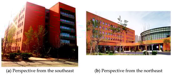
Figure 1.
The studied office building located on the campus.

Table 1.
Detailed building information.
Table 2.
Constitution and thermal properties of building envelope.
In the model, the total number of people in the building was 325; the work time was set as AM 7:00–PM 6:00 from Monday to Friday; the lighting load was 13 W/m2, 80% of which was instantaneous convection heat; the indoor heat source was mainly 200 computers with each 200 watts of power; the GSHP system was turned on only during working days.
2.2. Simulation of the Hourly Load of the Building
The hourly load of the building is the basis for the dynamic analysis of the air conditioning system. The commonly used simulation pieces of software are DOE-2, DeST, Energyplus, e-Quest, TRNSYS, etc. Among them, TRNSYS has flexible adaptability, and the simulation models built are quite realistic. TRNSYS is software for simulating transient processes of equipment. The most important feature of TRNSYS is its modular development and design format. When simulating a system, it is only necessary to call the corresponding functional components, set the parameters of each component according to the given conditions, and establish the connection relationship between each input and output signal to build a complete system. We used TRNBulid, an interface of TRNSYS, to calculate the loads of buildings. TRNBuild is a model-building partition of TRNSYS to obtain model-load information, mainly through the model building and the influences of characteristics of the model. TRNBuild can perform load calculations for complex partitions. Two modules were used most in the calculations for the model, i.e., time-meteorological parameters and the building load module. Meteorological data of the standard TM2 format numbered as Type 109 was used in the meteorological parameter module. The load calculation model established by TRNSYS is shown in Figure 2.
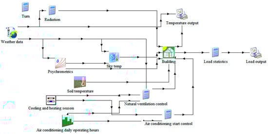
Figure 2.
Simulation flow chart of the building load calculation model.
The simulation results of building load are shown in Figure 3. The simulation results show that the peak heating load of this office building is 402.22 Kw, and the peak cooling load is 653.59 kW. The heating load of this building is concentrated in November to March, and the cooling load is concentrated in May to September. The air-conditioned area of the building is 9596.46 m2. The heating period is from 15 November to 15 March of the next year and the cooling time period is from 15 May to 15 September. The annual cumulative cooling load is 352,763.3395 kWh, and the annual cumulative heating load is 160,559.4867 kWh. According to the load calculation results, the heating and cooling loads per square meter are 41.91 and 67.11 W/m², respectively.
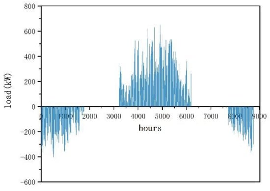
Figure 3.
The building’s hourly load.
3. Model Establishment
3.1. GSHP System Model
As depicted in the above sections, the peek cooling load of the building is larger than the peek heating load. The system should be designed according to the peek cooling load. The single U-shaped underground heat exchanger with a pipe diameter of DN32 was adopted for the system. Its vertical buried pipe depth was 100 m. According to the load, geotechnical thermal parameters, and design specifications [20], the total length of the borehole was calculated to be 12,340.58 m. Finally, 124 heat exchanger boreholes were designed with depth of 100 m.
The annual cumulative heat load of the system is greater than the annual cumulative cooling load. Considering the equilibrium soil temperature and the low tap-water temperature in winter, the domestic hot water in the heating season is borne by the ground-source heat pump system. A tank with a volume of 3.6 m3 was taken used.
The GSHP system is composed of a series of user-load circulation components and a series of ground-source-load circulation components. The specific components are shown in Figure 4. All component parameters were calculated and selected within the program’s specifications area. In addition, some basic conditions have to be set for the system as follows.
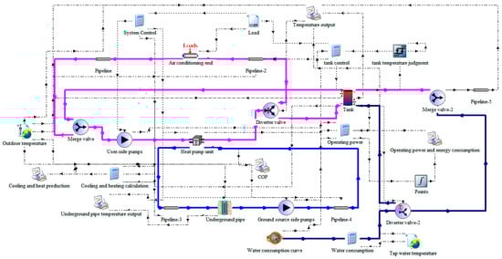
Figure 4.
TRNSYS model diagram of the GSHP system.
(1) The user-load water supply temperature of the heat pump unit in cooling mode was set as 7 °C, and the temperature for heating mode was set as 50 °C;
(2) The heat loss of the fluid in the connecting pipe was ignored, and circulating water temperature variation due to heat loss from the water pump was ignored.
3.2. System Operation Description
- The simulation time period was 0–8760 h, and the simulation step size was 0.125 h.
- When the heating load is greater than 10% of the rated heating capacity of the unit, the heat pump starts to heat the area. When the cooling load is greater than 10% of the rated cooling capacity of the unit, the heat pump starts to cool the area.
- Part of the tap water enters the water tank, and part enters the water point, where it is mixed, and the water temperature is controlled at 45 °C.
4. Optimization of the Operation Strategy
4.1. Optimization of Water Supply’s Temperature for the Load Side
When the load of the system is certain, the efficiency of the equipment varies with the temperature of the water supply [21]. At this time, the water supply’s temperature is within a reasonable range of variation. In fact, air conditioning systems operate under a partial load for most of the time. Therefore, a variable water temperature control strategy was set up for different load ratio situations and compared with a constant water supply temperature control strategy.
The system partial load ratio is calculated by the following formula:
in which is the actual cooling (heating) capacity, kW; is the design cooling (heating) quantity of the system, kW.
The regulation strategy of the water supply temperature is depicted as follows:
Cooling season:
Heating season:
in which is the water supply temperature of the load-side, °C; a and b are unknown parameters.
For the cooling season, when the load ratio was less than 20%, the water supply temperature of the load-side was set be 12 °C. When the load ratio was 100%, the water supply temperature was set to 7 °C. In the heating season, when the load ratio was less than 20%, the water supply temperature of the load-side was defined as 45 °C. When the load ratio was 100%, the water supply temperature was defined to be 50 °C. The water supply temperature was adjusted linearly within the load ratio interval of 20–100%. The specific temperature settings at different loading ratios are shown in Table 3.
Table 3.
Water supply temperature at different load ratios.
The annual power consumption of the GSHP system was obtained by TRNSYS simulation based on the set values of the constant and variable water supply temperature. A comparison of the two strategies is shown in Figure 5.
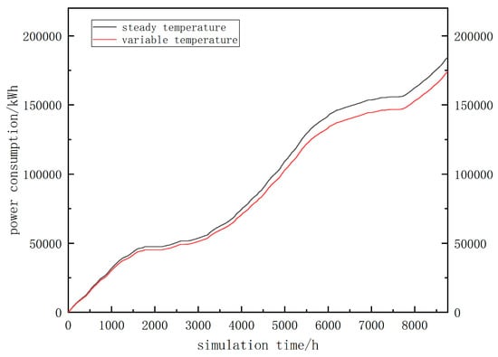
Figure 5.
Comparison of annual power consumption of the system with constant and variable water supply temperatures.
As can be seen in the above figure, the system ‘senergy consumption is significantly lower under the variable water supply temperature strategy compared with the constant water supply temperature strategy.
4.2. Water Supply Temperature Optimization Based on User-Load of the Units Using TRNSYS-GENOPT (TRNOPT)
The performance of the main energy-consuming equipment of the air conditioning system at different load ratios is affected to various degrees by changes in the water supply’s temperature. The air conditioning system operates at different load ratios, corresponding to different optimal water supply temperatures, which can make the whole system operate at that operating state with the lowest energy consumption [21].
To obtain the optimal water supply temperature, the water supply temperature on the load side was used as a variable value with the load ratios of 20% and 100%. Then, the variables were optimized by the TRNOPT module of TRNSYS software. The optimal water supply temperature value for the load side of the unit could be obtained. The optimization process included the following steps, i.e., (1) Define independent variables successively. (2) Determine the objective function. (3) Specify constraints on optimization variables. (4) Determine the initial value and iteration step. (5) Choose the optimization algorithm. (6) Get the value of the optimal independent variable.
4.2.1. Optimized Setting of Water Supply Temperature
The water supply temperature regulation strategy of the load-side based on TRNOPT optimization is as follows:
Cooling season:
Heating season:
in which is the water supply temperature of the load-side, °C; e and f are unknown parameters.
In the cooling season, when the load ratio is less than 20%, the water supply temperature was defined as variable . When the load ratio is 100%, the water supply temperature is defined as variable . In the heating season, when the load ratio is less than 20%, the water supply temperature is defined as variable . When the load ratio is 100%, the water supply temperature is defined as variable . The water supply temperature is adjusted linearly within the load ratio interval of 20–100%.
The increase in the evaporator outlet temperature in cooling season and the decrease in the condenser outlet temperature in the heating season have obvious effects on reducing the energy consumption of the unit and improve the energy efficiency of the system. However, if the evaporator’s outlet temperature is set too high or the condenser’s outlet temperature is set too low, the indoor thermal comfort level will be reduced. In order to satisfy the cooling and heating needs of the building and the comfort of the users, and also ensure the normal operation of the heat pump, the outlet temperature range of the evaporator was set to 5–15 °C during the cooling season, and the outlet temperature range of the condenser was set to 40–50 °C during the heating season [22]. The parameter optimization settings are shown in Table 4.
Table 4.
Parameter optimization settings.
No matter how the system is optimized, energy savings should not come at the cost of reduced indoor thermal comfort. Moreover, it is a challenge to save energy under the promise of proper thermal comfort because there is a conflicting relationship between energy efficiency and thermal comfort. PMV (predicted mean vote) is an evaluation indicator that characterizes the body’s thermal response (hot and cold sensation). PMV is recommended to be between −0.5 and 0.5. Indoor air temperature and humidity can affect PMV [23,24,25,26,27,28]. Therefore, both indoor temperature and humidity should be constrained to ensure the thermal comfort of the room, so that the variables are always optimized within the acceptable range. The interior design temperature range was set as 24–26 °C, and relative humidity was less than 65% in summer, and the temperature was set to 19–21 °C without humidity restriction in winter. If the optimized variables cannot meet the indoor temperature or humidity requirements after turning on the air conditioner for one hour per day, the penalty energy consumption is added to the energy consumption under the operation of this variable. The reason for setting one hour here is that when the air conditioner is first turned on, the room temperature and humidity cannot immediately meet the design requirements. When the minimum indoor temperature is lower than 19 °C in the heating season, or the maximum indoor temperature exceeds 26 °C or the relative humidity exceeds 65% in the cooling season, the penalty energy consumption should be increased.
The optimization objective function is:
in which T means room temperature, °C; RH represents room relative humidity; denotes total system energy consumption, kWh; denotes the penalty energy consumption in the cooling season, kWh; is the penalty energy consumption in the heating season, kWh.
The TRNOPT optimization module, the independent variable setting calculation module and the objective function calculation module were added to the model that was already established in the TRNSYS platform. In addition, cooling and heating cycles between the building module and the fan coil module were used to represent the load demand of the building. When optimizing operating parameters, indoor temperature and humidity can be controlled to ensure building comfort. The building load simulation module Type56 in TRNSYS was used as the building cooling and heat consumption module of the research subject. The building shape, envelope parameters, indoor thermal disturbance and other parameters were input into the building module according to the actual situation. The envelope parameters and thermal disturbances were set according to the parameters in Section 2.1. The Type753 module was used for the fan coils. In this study, only the water supply temperature of the unit was optimized, and the operation and energy consumption of the fan coil were not considered. In order to simplify the model and improve the simulation speed, all fan coil units of the system were considered as a whole unit. The TRNOPT optimization model of the GSHP system was built as shown in Figure 6. Based on the TRNOPT optimization platform, the optimal water supply temperature setting value was searched based on the aforementioned definitions of independent variables, constraints, and objective functions. The total system energy consumption corresponding to the optimal water supply temperature was simulated by the established model.
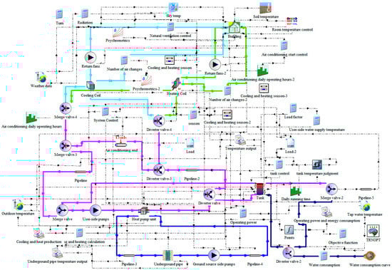
Figure 6.
Model constructed on the TRNOPT optimization platform.
In the TRNOPT procedure, the Hooke-jeeves algorithm is used as the optimization method, which is mainly composed of alternating “probe search” and “mode movement”. The starting point of the probe search (initial setpoint) is the reference point. The aim is to find a better point around the reference point and thus determine a favorable direction of progress. At the same time, the step size is constantly reduced, and the search for the best continues. Hooke-jeeves used generalized pattern search (GPS) algorithm to evaluate the adaptive accuracy function. To simplify the implementation,
The search direction matrix is defined as:
Parameter is used to calculate the mesh size parameter . The mesh size is defined by the Mesh Size Divider; The initial Mesh Size Exponent is defined by the Initial Mesh Size Exponent. If the control goal is not reduced in the repeated computation, the exponential increment of the mesh size is specified by the parameter of Mesh Size Exponent Increment.
In the Hooke-Jeeves algorithm, whenever the target parameter that is set in this calculation (energy consumption) is found to be lower than the previous one, the next optimization value is shifted in the direction of this parameter that makes the target parameter lower. At this point, the algorithm finds the point of the new cycle, which is also the point in the GPS model algorithm.
Hooke-Jeeves algorithm parameter settings are shown in Table 5.
Table 5.
Hooke-Jeeves algorithm parameter settings.
4.2.2. Optimization Results and Analysis
The results of optimization of water supply temperature based on TRNOPT were as follows. The execution time of the study method was 337 min. The execution time is related to the computer configuration. The computer configurations used in this study are listed in the Table 6 below.
Table 6.
Computing configuration information.
The optimized water supply temperature settings based on TRNOPT are shown in Table 7. For the cooling season, when the load ratio was less than 20%, the water supply temperature was set to 11.4 °C, and for the load ratio of 100%, the water supply temperature was set to 7.6 °C. During the heating season, when the load ratio was less than 20%, the water supply temperature was set to 43.8 °C, and for the load ratio of 100%, the water supply temperature was set to 48.3 °C. The water supply temperature is adjusted linearly within the load ratio interval of 20–100%.
Table 7.
Water supply temperature setting values before and after optimization based on TRNOPT.
According to the set values of the above three water supply temperature schemes, the GSHP system built in TRNSYS platform was run. The comparison of the annual operating power consumption of the three schemes is shown in Figure 7. A comparison of the difference in the annual operating energy consumption between the TRNOPT-based optimization scheme and the other two schemes is shown in Figure 8.
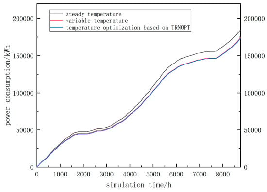
Figure 7.
Comparison of the annual power consumption of the system under three water supply temperature schemes.
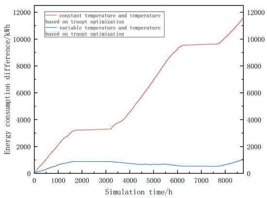
Figure 8.
Comparison of the annual energy consumption between the third water supply temperature scheme and the other two schemes.
From the above two figures, it is obvious that the energy consumption of the system under the TRNOPT optimized water supply temperature scheme is decreased significantly compared with that under the constant water supply temperature scheme. Additionally, there is also a certain decrease in energy consumption compared with that of the variable supply temperature scheme.
The total annual operating energy consumption of the system under the three water supply temperature schemes was obtained as shown in Table 8.
Table 8.
Annual total energy consumption under the three water supply temperature schemes.
According to the energy consumption comparison data in the above table, it can be seen that the total annual energy consumption under the variable water supply temperature scheme was less than that under the constant water supply temperature scheme by 10,531.41 kWh. The energy saving ratio was about 5.7%. The total annual energy consumption under the optimized water supply temperature based on TRNOPT was lower than that under the variable water supply temperature scheme by 1072.04 kWh, and it was lower than that under the constant water supply temperature scheme by 11,603.45 kWh. The energy saving ratio was about 6.3%. The water supply temperature strategy based on TRNOPT optimization proposed in this study determines the optimal water supply temperature of the system. In practical engineering, the constant water supply temperature strategy is more common. The proposed strategy takes into account the transient variation characteristics of the actual load compared with the constant water supply temperature strategy. Currently, the variable supply temperature strategy is more frequently studied. The water supply temperature strategy based on TRNOPT optimization takes into account the thermal comfort of the room compared with the variable water supply temperature strategy. By comparing the three strategies, the TRNOPT-based optimized water supply temperature strategy is the best water supply temperature strategy. In addition, the execution time of the proposed method was 337 min, which denotes high computational efficiency.
Therefore, the optimization results based on TRNOPT were finally selected as the optimal water supply temperatures, which can supply thermal comfort and reduce the energy consumption of the system’s operation simultaneously.
5. Conclusions
In this study, a TRNSYS load calculation model was firstly established according to the relevant information of an office building located in Jinan, and then a GSHP system model was established on the TRNSYS platform. Considering that the air conditioning systems mostly operate under partial-load conditions, the method of setting a constant water supply temperature often leads to wasteful power consumption by the system. Therefore, a variable water temperature control strategy was created according to the different load ratios of the heat pump units. When the load ratio is between 20% and 100%, the water supply temperature is set accordingly. The water supply temperature is adjusted linearly within the load ratio interval of 20–100%.
Through TRNSYS simulation, the total annual energy consumption under the variable water supply temperature scheme was less than that under the constant water supply temperature scheme by 10,531.41 kWh. The energy saving ratio was about 5.7%. For further optimization, the water supply temperature scheme based on TRNOPT optimization was proposed to find the optimal water supply temperature under different load ratios, which can minimize the energy consumption of the system and satisfy the thermal comfort of the room. Finally, the optimal setting values for the water supply temperature when the load factor is less than 20% and when the load factor is 100% were obtained.
The simulation results show that the total annual energy consumption under the optimized water supply temperature based on TRNOPT is lower than that under the variable water supply temperature scheme by 1072.04 kWh, and it is lower than that under the constant water supply temperature scheme by 11,603.45 kWh. The annual energy saving ratio of the system is about 6.3%. It is concluded that the optimized water supply temperature scheme based on TRNOPT has a better energy saving effect than the first two water supply temperature schemes. The strategy proposed in this study is the optimal water supply temperature strategy, which determines the optimal water supply temperature of the system. By optimizing the operation of the GSHP system, it can provide good reference values and guidance for an actual project, thereby promoting the efficient application of GSHP energy-saving technology to actual projects. The limitation of this work is the lack of experimental validation of the simulation study results. The building was equipped with a monitoring system. However, we could not obtain the actual running data, since the monitoring system could not work validly. In the next cooling season, we will try to measure the GSHP system to verify the simulation data.
Author Contributions
Conceptualization, J.C. and S.Z.; methodology, S.Z.; software, J.C.; investigation, T.W., B.S. and X.L.; formal analysis, J.C.; resources, T.W.; data curation, B.S.; writing—original draft preparation, J.C.; writing—review and editing, S.Z. All authors have read and agreed to the published version of the manuscript.
Funding
This research received no external funding.
Institutional Review Board Statement
Not applicable.
Informed Consent Statement
Not applicable.
Data Availability Statement
Not applicable.
Acknowledgments
This work acknowledges the Plan of Introduction and Cultivation for Young Innovative Talents in Colleges and Universities of Shandong Province.
Conflicts of Interest
The authors declare no conflict of interest.
References
- Xu, W.; Zhang, S. Current situation and development trend of Chinese GSHP technology. Sol. Energy 2007, 3, 11–14. [Google Scholar]
- Bozgeyik, A.; Altay, L.; Hepbasli, A. A sub-system design comparison of renewable energy based multi-generation systems: A key review along with illustrative energetic and exergetic analyses of a geothermal energy based system. Sustain. Cities Soc. 2022, 82, 103893. [Google Scholar] [CrossRef]
- Walch, A.; Li, X.; Chambers, J.; Mohajeri, N.; Yilmaz, S.; Patel, M.; Scartezzini, J.-L. Shallow geothermal energy potential for heating and cooling of buildings with regeneration under climate change scenarios. Energy 2022, 244, 123086. [Google Scholar] [CrossRef]
- Arat, H.; Arslan, O. Exergoeconomic analysis of district heating system boosted by the geothermal heat pump. Energy 2017, 119, 1159–1170. [Google Scholar] [CrossRef]
- Lmmle, M.; Bongs, C.; Wapler, J.; Günther, D.; Hess, S.; Kropp, M.; Herkel, S. Performance of air and ground source heat pumps retrofitted to radiator heating systems and measures to reduce space heating temperatures in existing buildings. Energy 2022, 242, 122952. [Google Scholar] [CrossRef]
- Zhang, H.; Han, Z.; Li, G.; Ji, M.; Cheng, X.; Li, X.; Yang, L. Study on the influence of pipe spacing on the annual performance of ground source heat pumps considering the factors of heat and moisture transfer. seepage and freezing. Renew. Energy 2021, 163, 262–275. [Google Scholar] [CrossRef]
- Zhu, S.; Sun, J.; Zhong, K.; Chen, H. Numerical Investigation of the Influence of Precooling on the Thermal Performance of a Borehole Heat Exchanger. Energies 2021, 15, 151. [Google Scholar] [CrossRef]
- Yin, Y.; Zhu, D.; Wang, N. Selection of water chiller units and energy consumption of water system. Heat. Vent. Air Cond. 2009, 39, 94–97. [Google Scholar]
- Chen, M. Impact Analysis of Chilled Water Temperature Control on Energy Consumption of Central Air Conditioning Plants. Build. Energy Environ. 2012, 31, 64–66. [Google Scholar]
- Thu, K.; Saththasivam, J.; Saha, B.B.; Chua, K.J.; Murthy, S.S.; Ng, K.C. Experimental investigation of a mechanical vapour compression chiller at elevated chilled water temperatures. Appl. Therm. Eng. 2017, 123, 226–233. [Google Scholar] [CrossRef]
- Ukai, M.; Tanaka, H. A case study of a pilot system with gas-engine heat pumps and a desiccant air handling system using higher chilled water temperature in Japan. Appl. Therm. Eng. 2022, 201, 117817. [Google Scholar] [CrossRef]
- Bai, M.; Wang, F.; Liu, J.; Wang, Z. Experimental and numerical studies of heat and mass transfer performance and design optimization of Fan-coil with high supply chilled water temperature in Air-Conditioning system. Sustain. Energy Technol. Assess. 2021, 45, 101209. [Google Scholar] [CrossRef]
- Wang, L.; Lee, E.W.; Yuen, R.K. A practical approach to chiller plants’ optimization. Energy Build. 2018, 169, 332–343. [Google Scholar] [CrossRef]
- Sala-Cardoso, E.; Delgado-Prieto, M.; Kampouropoulos, K.; Romeral, L. Predictive chiller operation: A data-driven loading and scheduling approach. Energy Build. 2020, 208, 109639. [Google Scholar] [CrossRef]
- Chang, Y.-C.; Chen, W.-H. Optimal chilled water temperature calculation of multiple chiller systems using Hopfield neural network for saving energy. Energy 2009, 34, 448–456. [Google Scholar] [CrossRef]
- Karami, M.; Wang, L. Particle Swarm Optimization for Control Operation of an All-Variable Speed Water-Cooled Chiller Plant. Appl. Therm. Eng. 2018, 130, 962–978. [Google Scholar] [CrossRef]
- Thangavelu, S.R.; Myat, A.; Khambadkone, A. Energy optimization methodology of multi-chiller plant in commercial buildings. Energy 2017, 123, 64–76. [Google Scholar] [CrossRef]
- Qiu, S.; Li, Z.; Li, Z.; Zhang, X. Model-free optimal chiller loading method based on Q-learning. Sci. Technol. Built Environ. 2020, 26, 1100–1116. [Google Scholar] [CrossRef]
- Qiu, S.; Li, Z.; Fan, D.; He, R.; Dai, X.; Li, Z. Chilled water temperature resetting using model-free reinforcement learning: Engineering application. Energy Build. 2022, 255, 111694. [Google Scholar] [CrossRef]
- Wei, X.; Yu, Z. Engineering Technical Specification for GSHP System, 2nd ed.; China Academy of Building Sciences: Beijing, China, 2009; pp. 9–10. [Google Scholar]
- Meng, Q.L.; Zhang, Z.B. Simulation study on the operation effect of variable water temperature strategy for variable air volume air conditioning system. J. Syst. Simul. 2019, 31, 1617–1626. [Google Scholar]
- Sun, R. Research on Load Prediction and Control Strategy of Efficient Refrigeration Room Based on Particle Swarm Optimization. Master’s Thesis, Qingdao Technological University, Qingdao, China, 2021. [Google Scholar]
- Li, Y.; Han, M.; Shahidehpour, M.; Li, J.; Long, C. Data-driven distributionally robust scheduling of community integrated energy systems with uncertain renewable generations considering integrated demand response. Appl. Energy 2023, 335, 120749. [Google Scholar] [CrossRef]
- Fang, J.; Feng, Z.; Cao, S.-J.; Deng, Y. The impact of ventilation parameters on thermal comfort and energy-efficient control of the ground-source heat pump system. Energy Build. 2018, 179, 324–332. [Google Scholar] [CrossRef]
- Wan, T.; Bai, Y.; Wang, T.; Wei, Z. BPNN-based optimal strategy for dynamic energy optimization with providing proper thermal comfort under the different outdoor air temperatures. Appl. Energy 2022, 313, 118899. [Google Scholar] [CrossRef]
- Gao, J.; Yan, J.; Xu, X.; Yan, T.; Huang, G. An optimal control method for small-scale GSHP-integrated air-conditioning system to improve indoor thermal environment control. J. Build. Eng. 2022, 59, 105140. [Google Scholar] [CrossRef]
- Martins, N.R.; Bourne-Webb, P.J. Providing renewable cooling in an office building with a Ground–Source heat pump system hybridized with natural ventilation & personal comfort systems. Energy Build. 2022, 261, 111982. [Google Scholar]
- Ye, M.; Nagano, K.; Serageldin, A.A.; Sato, H. Field studies on the energy consumption and thermal comfort of a nZEB using radiant ceiling panel and open-loop groundwater heat pump system in a cold region. J. Build. Eng. 2023, 67, 105999. [Google Scholar] [CrossRef]
Disclaimer/Publisher’s Note: The statements, opinions and data contained in all publications are solely those of the individual author(s) and contributor(s) and not of MDPI and/or the editor(s). MDPI and/or the editor(s) disclaim responsibility for any injury to people or property resulting from any ideas, methods, instructions or products referred to in the content. |
© 2023 by the authors. Licensee MDPI, Basel, Switzerland. This article is an open access article distributed under the terms and conditions of the Creative Commons Attribution (CC BY) license (https://creativecommons.org/licenses/by/4.0/).