Abstract
This article discusses the challenges of water scarcity and industrial water pollution in developing countries, specifically in Morocco, where the olive oil industry is a significant contributor to organic water pollution. The Moroccan government has implemented regulations and economic incentives to address this issue, but enforcement has been hindered by a lack of information on environmental damage and pollution abatement costs. This study aims to improve the knowledge of public decision makers on the costs of the depollution of oil mills and to use this information to develop tools for the reinforcement of the current regulation mechanism. To meet our research objective, the Translog hyperbolic distance function is used to represent the environmental technology generating three undesirable outputs (SS, BOD, and COD) and to estimate the olive oil mills’ specific pollution abatement cost (shadow price). Finally, pollutant-specific taxes are computed using the tax-standard method. The results showed that oil mills must renounce the production of olive oil totaling MAD 13,314, MAD 4706, and MAD 5786 for the reduction of one ton of SS, BOD, and COD, respectively, and that there are economies of scale in the treatment of olive mill wastewater. After calculating the rate of the environmental tax, we conclude that implementing the tax according to current emission standards can be very restrictive for oil mills, as it would represent 22% of the total annual turnover of the olive oil industry. These findings suggest a redesign of the regulation mechanism, including the implementation of environmental monitoring systems, the consideration of economies of scale in pollution control, and the use of better-targeted green subsidies and effective environmental tax. However, further research is needed to understand the impact of these measures on the economic performance of the olive oil industry.
1. Introduction
Water scarcity and industrial water pollution are significant challenges facing many developing countries where regulations may be less strict, and enforcement may be weaker than in developed countries [1,2]. This can lead to significant environmental damage and harm to public health. In Morocco, the olive oil industry is a significant contributor to organic water pollution [3]. For an annual mean olive production of 1.3 million tons (2014–2018), the Moroccan olive processing sector generates more than 1 million m3/year of olive mill wastewater (OMWW) [4]. These effluents are characterized by a very high organic load, an acid pH, and a low biodegradability [5,6]. According to the audit mission of the olive sector conducted by the Moroccan Court of Account, it was found that 88% of olive oil mills do not comply with the evacuation standards of OMWW. In the majority of cases, these effluents are stored in basins that do not comply with the technical standards and, after storage, are either clandestinely discharged into the natural environment, or directly into the sewerage system. The OMWW constitutes a serious environmental constraint that endangers water resources due to the effluents discharged without prior treatment in the water courses and the public sewage system [7].
To deal with this scourge, like other countries in the Mediterranean basin, Morocco, since the 2000s, has adopted a mechanism to control water pollution by OMWW. This mechanism is based mainly on two types of instruments: regulatory instruments and economic instruments. The first regulatory instrument, also called a command and control instrument, consists of subjecting any industrial discharge into surface or groundwater to a discharge authorization issued by the Hydraulic Basin Agency (HBA). With this authorization, industrialists are required to comply with emission standards called discharge limit value (DLV). The second economic instrument is based on a subsidy for pollution reduction granted exclusively to the creation of two-phase oil mills or to the conversion of oil mills from a three-phase to a two-phase process. However, the implementation of this environmental regulation mechanism is hampered by two constraints. The first constraint is the difficulty of setting up a compliance control system for oil mills, which requires high administrative costs for managing the environmental monitoring system. The second informational constraint is related to the lack of information on the environmental damage and on the abatement cost of oil mills [8].
The lack of a rigorous environmental control system and the situation of information asymmetry in the disfavor of the regulator considerably reduces the efficiency of its environmental regulation mechanism [9,10]. These facts and weaknesses plead in favor of a reform of the current mechanism of industrial water pollution control based essentially on the regulatory approach that can be qualified as a “Command without Control” system.
The debate on the choice of environmental regulation instruments has fueled a large literature that has focused on the effectiveness of the command and control regulatory approach compared to the approach based on economic instruments [11,12,13,14,15,16]. Baumol [11] states that in a situation of uncertainty on environmental damage where the optimum is inaccessible, the environmental tax constitutes an efficient alternative from an economic viewpoint to a uniform emission standard. Likewise, Tietenberg [17] and Stavins [15] confirm that the use of economic instruments, namely the environmental tax, makes it possible to achieve the environmental target set while providing incentives for producers and polluters to take advantage of emission abatement opportunities at the lowest cost. However, if the superiority of the environmental tax over the emission standard has been proven easily in theory, the loosening of the assumption of perfect information on the costs of pollution abatement may complicate the determination of the tax rate. Indeed, although information on the marginal abatement cost is very useful for the public authority (regulatory), it is generally not accessible. This is because the undesirable joint product is rarely marketed, and therefore, they are rarely priced [18].
The concept of shadow price is a key tool to approach the marginal abatement cost of undesirable production. Using the distance functions and duality theory, the shadow price of the undesirable product can be derived from the market price of the desirable output. The shadow price concept has been widely used in the literature to estimate the marginal abatement cost [18,19,20,21]. Studies on water pollution have focused on various productive activities in different countries: the paper industry in Canada [22]; the sugar industry in India [23]; the ceramic industry in Spain [24]; the rubber industry in Sri Lanka [25]; the chemical, textile, and food industry in Sri Lanka [26]; the leather industry in India [27]; the agricultural sector in China [28]; and the textile industry in China [29]. It results from this literature review that the applications in developing countries are relatively important because water pollution is considered the main pollution problem in these countries [30]. This situation is aggravated by the context of water scarcity, especially in countries suffering from a succession of drought episodes and lax environmental regulations [8,31]. However, it should be noted that despite the diversity of industrial activities covered by these cited empirical studies, the economic literature on interventions to control water pollution by OMWW is inexistent. Despite the serious environmental problem posed by the olive oil industry, the literature on pollution generated by oil mills has been limited to the characterization of OMWW and the physical quantification of their impact on water resources [32,33,34,35,36,37]. This article is thus the first contribution to the economic analysis of the regulation instruments of water pollution resulting from the olive oil industry in Morocco and in the Mediterranean basin in general.
In order to reduce the informational constraint faced by the regulator, this study aims to first estimate the abatement costs at each oil mill. Considering the pressing will of the Moroccan government to improve water quality in the current context marked by the scarcity of the resource, which was concretized by the initiation of a National Program to control water pollution by OMWW, we chose to extend our analysis to the scope of the regulation mechanism and the development of tools for its reinforcement, notably by designing an environmental tax that would encourage olive oil producers in Morocco to comply with environmental standards.
To meet the objectives of this study, we chose to combine the parametric hyperbolic distance function and the tax-standard method. Using this combined approach, we will first model the environmental technology by taking into account the undesirable joint production of three organic pollutants: suspended solids (SS), biochemical oxygen demand (BOD), and chemical oxygen demand (COD). This first step aims to evaluate and analyze the environmental performance of Moroccan oil mills under the effect of the current environmental regulation system. Afterward, we will use the duality between the distance function and the profitability function to calculate the shadow prices for the three considered pollutants, and we will define the pollution abatement cost functions accordingly. Finally, by adopting the tax-standard approach of [11], the information on the marginal abatement cost estimated for the oil mills will be used as a guideline to design the level of the environmental tax that will lead olive oil producers to respect the current emission standards (DLV).
The contribution of this study is twofold. First, it provides an estimate of pollution abatement costs in a specific developing country context focusing on the olive oil industry, which has not been extensively studied. Secondly, it offers insights to policymakers, and proposes a regulation mechanism with an integrated approach that includes a combination of regulatory and incentive measures to reduce water pollution from oil mill activity.
The remainder of this paper is structured as follows: Section 2 provides a review of the literature; Section 3 presents the methodology adopted in this study and describes the data used; Section 4 interprets and discusses the empirical results. Finally, Section 5 concludes and proposes some orientations in terms of public policies.
2. Literature Review
The polluting industrial emissions are considered negative externalities of production, also called undesirable productions. In the presence of its joint productions, the productive process generates simultaneously desirable and undesirable productions. The integration of these undesirable outputs in the production process modeling makes radial distance functions inappropriate [20]. Indeed, the radial distance direction output tends to maximize all outputs produced, including undesirable outputs, whose production is undesired or not allowed by the environmental regulation that is imposed on production units. The question of “how” to take into account undesirable outputs in the modeling of production technology has been the subject of several research studies. Several publications have been identified by Zhou et al. [38] and Song et al. [39] covering the subject between 1983 and 2011. The review of these studies and more recent ones allowed us to identify three approaches used for modeling undesirable outputs in the production process.
The first approach described in the works [22,40,41] consists of considering desirable outputs as inputs. This methodology has several theoretical limitations that make its application restricted. Indeed, when undesirable outputs are treated as inputs, it is always possible to increase undesirable products for a given amount of input and desirable output. Thus this approach does not consider any relationship between the production of undesirable outputs and the use of inputs [42].
Another approach is proposed by [41,43] in which they propose to proceed by transformations of variables. It consists of modifying the undesirable outputs by using a monotone decreasing function. This transformation aims to integrate the undesirable outputs with the desirable ones and to maximize them as classical productions by ensuring that the most polluting firms are the least efficient. The most appropriate function to perform this transformation has been the subject of several theoretical debates [43,44].
The approach most adopted by recent studies [18,19,27,45,46,47] uses non-radial distance functions to overcome the limitations of the radial type of measurements classically used. The hyperbolic distance function introduced by [48] and the directional distance function developed by [49] allow an asymmetric treatment between different inputs, desirable outputs, and undesirable outputs, thus defining the polluting productive activities in a multidimensional analysis framework. With this key asset, the non-radial distance function remains one of the most appropriate theoretical tools in the quest for a tradeoff between the firm’s productive performance and its environmental performance.
The estimation of distance functions can be performed using two methods: parametric and non-parametric. The non-parametric method developed by [50], also called the DEA method “Data Envelopment Analysis”, uses mathematical programming techniques and does not impose a particular functional form on the distance function. Nevertheless, the DEA technique does not take into account the stochastic variance from the frontier; the results obtained are, therefore, very sensitive to outliers [51]. Moreover, the distance function estimated using DEA is not differentiable, so it is not adapted to derive the shadow price [20]. In contrast to the non-parametric method, the parametric method associates a functional form with the distance function, and the parameters of this function are estimated by linear programming. This method takes into account statistical noise and has the advantage of being differentiable and not very sensitive to outliers [28].
The recent development of distance functions in the modeling of undesirable non-market outputs allows estimating the marginal abatement costs of pollutants produced jointly with desirable output without market price information.
The recent development of distance functions in the modeling of undesirable non-market outputs allows estimating the marginal abatement costs of pollutants produced jointly with desirable output without market price information.
The shadow price is a promising approach for estimating the marginal abatement cost and has been popularized by [52,53,54] and adopted by many authors [23,24,45,47,55,56,57,58]. Resulting from the duality between distance functions and cost, revenue, or profit functions, the shadow price of undesirable joint production can be interpreted as the opportunity cost of reducing an additional unit of this undesirable output in terms of loss in the production of desirable output [52]. The advantage of this approach proposed in the pioneering work of [52] is that it does not require any information about regulatory constraints. Indeed, in the framework of duality theory, the estimation of the shadow price of the undesirable output allows the economic evaluation of the technological opportunity cost resulting from the primal representation of the technology [18].
Estimating the shadow price of a pollutant provides policymakers with useful information for the design of an effective environmental regulation mechanism. Considering the shadow price as a reference value, regulators can design an optimal environmental tax regime to control polluting emissions from firms. The shadow price also has the advantage of verifying whether all firms face the same marginal abatement cost [59]. At the microeconomic level, the availability of information on the shadow price makes it possible to help producers make decisions about investments in pollution control [24].
3. Methodological Development
3.1. Theoretical Model
In this study, we adopted the parametric hyperbolic distance function as a first step to evaluate the environmental performance of oil mills. Subsequently, we deduced the shadow price of the undesirable output using the duality relationship between the hyperbolic distance function and the profitability function.
3.1.1. The Parametric Hyperbolic Distance Function
The hyperbolic distance function proposed by [48], as an extension of Shephard’s radial measure, allows for a simultaneous and equal-proportional adjustment in inputs and outputs in order to reach the production technology frontier. Considering a joint production technology with partitioning of the outputs into polluting (undesirable) and non-polluting (desirable) components, the hyperbolic measure provides an adequate tool for the representation of our environmental technology.
Consider a production technology using the input vector to produce a vector of desirable outputs and a vector of undesirable outputs where the subscript refers to the set of firms observed. Given the particular properties of joint production, we adopt the production set described below to model the environmental production technology:
Assuming that this set of production possibilities is compact and verifies the standard axioms posed by [60], it is also possible to represent the production technology by the hyperbolic distance function. This function inherits its name from the hyperbolic path it follows, which translates the distance between each observation and the frontier of the production set P(x).
The hyperbolic measure expresses simultaneously, for a given quantity of inputs, the maximum expansion of the vectors of desirable outputs and the equal-proportional contraction of the vectors of undesirable outputs and placing the firm in the production frontier. Referring to the works [18,61], the hyperbolic distance function is defined by the following:
When , this implies that the observed firm is at the frontier of the set of production possibilities and that it is not more possible for it to reduce its production of undesirable output without reducing its production of desirable goods; the firm is thus considered fully efficient. Furthermore, if the firm is considered inefficient and requires efforts to improve its efficiency by increasing its production of desirable output and reducing undesirable output.
The hyperbolic distance function must satisfy a number of properties [18], namely that
- It is almost homogeneous in degrees 0, 1, −1, 1. This implies that for a given level of inputs, if the vector of desirable outputs increases by a given proportion, the vector of undesirable outputs decreases by the same proportion, and the distance function will increase by the same proportion. This property can be expressed as follows: ;
- It is non-decreasing in desirable outputs: ;
- It is non-increasing in undesirable outputs: ;
- It is non-increasing in inputs: .
Following the studies [18,45,47], the almost homogeneity property allows the transformation of the hyperbolic distance function into a normalized function using a desirable output as a numerary such as . After transformation the hyperbolic distance function can be expressed as follows:
By a switch to the logarithm on both sides of Equation (3), we obtain the following:
For the functional specification, and as previously mentioned, we chose the Translog form because of its flexibility compared to other specifications such as Cobb–Douglas or CES.
The mathematical expression for the Translog specification of the hyperbolic distance function is given by the following:
where and ; and , , , , and are parameters to be estimated.
Equation (5) cannot be directly estimated since is not directly observed. In the stochastic framework chosen for our study, the distance separating the producer from the production frontier can be considered the combined effect of two independent components: a first one purely random and a second one representing the productive inefficiency [62].
Considering and as dependent variable, we obtain by transformation of Equation (5) an estimable form of our model, expressed as follows:
where is the purely random error term that captures the statistical noise related to measurement errors not controlled by the producers, such as model specification errors or data omission errors. This error vector is assumed to be normally symmetrically distributed (two-sided error term) .
is the error term reflecting productive inefficiency. It is assumed to be positive, distributed on one side of the production frontier only (one-sided error term), and follows a semi-normal or exponential distribution .
3.1.2. Estimate of Shadow Price
The shadow price associated with the undesirable output can be deduced from the market price of the desirable output. Indeed, the duality between the distance functions and the cost, revenue, or profit functions makes it possible to obtain information on the costs of controlling the pollution generated by the production of undesirable outputs.
Referring to [18,45,47,58,60], we describe in this section the procedure for estimating the shadow price using Shephard’s Dual Lemma and the duality relation proved by [63] between the hyperbolic distance function of our environmental technology and the maximization of the profitability function.
The “Return to the dollar” measure provided by [64] is defined by where p is the price of output and the price of input . It should be noted that as long as is interpreted as observed revenue and as observed cost, it is not necessary to have information on prices in order to evaluate profitability through the “Return to the dollar” measure [63].
In this case study, we considered the two types of desirable outputs , and undesirable with their respective prices and (unknown); therefore, the profitability maximization problem will be expressed as follows:
By applying the Lagrangian method and the envelope theorem, the first-order conditions of the maximization problem are as follows:
Taking the ratio between these two conditions (8) and (9), we obtain the following:
The right side of Equation (10) can be expressed, on the frontier of the production set, as the slope of the relation between and . Thus, by applying the implicit function theorem on the hyperbolic distance function, we obtain the following:
The result can be interpreted as the economic opportunity cost of reducing an additional unit of undesirable output in terms of loss of production of desirable output when the point is situated on the production frontier. This result corresponds to the shadow price of b in terms of desirable production .
3.2. Study Area and Data Description
To conduct this study, we chose the Sebou hydraulic basin in Morocco, which is considered to be the basin most impacted by OMWW [7]. Oil mills are distributed across almost the entire basin, with marked concentrations in the provinces of Taounate, Meknes, El Hajeb, and Fes. The study area is represented in Figure 1.
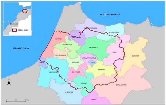
Figure 1.
Presentation of the study area.
The olive oil sector in the basin of Sebou includes more than 480 industrial units. In this empirical study, we based our analysis on data collected in an inventory study conducted by the ABHS, which covered all the industrial oil mills in its area of action. This database contains real and detailed data on the olive oil production process and on the amount of polluting discharge from the oil mills’ crushing activity. Excluding the units temporarily or permanently closed, the number of oil mills is 461 (122 oil mills adopting the two-phase system and 339 oil mills adopting the three-phase system). Due to limited data availability, we used cross-sectional data from the olive-crushing season of 2019/2020.
Taking into account the diversity of olive crushing processes, that is, three-phase process and two-phase process, and in order to obtain a homogeneous representation of our production technology, two desirable products were considered: olive oil and other productions. Jointly, oil mills produce three undesirable outputs: biochemical oxygen demand (BOD), chemical oxygen demand (COD), and suspended solids (SS). These products are obtained from the combination of four inputs, namely olives, other intermediate consumption represented by water and energy consumption, labor, and crushing capacity used as a proxy for capital.
Table 1 presents the descriptive statistics of the variables used in our analysis. It shows a high variability of the data marked by the large range between the maximum and minimum values of each variable. Since the sample size is proportional to the variability of the data, this size was pushed to its maximum, thus justifying our choice to adopt an exhaustive sampling (census).

Table 1.
Descriptive statistics.
Given this high data variability and in order to ensure that the mean values do not mask variations in the data that may be due to the internal characteristics of the oil mills, we chose to split these mean values by type of process and by mill size (maximum crushing capacity) in order to have a summary description of the data.
Table 2 shows that the two-phase and three-phase oil mills represent 26% and 74% of our exhaustive sample, respectively. The medium-sized oil mills with a maximum crushing capacity between 13 and 15 tons/day represent nearly 50% of the oil mills studied for the two types of processes considered. Large oil mills with a maximum capacity of 15 tons/day represent 31% of all two-phase oil mills and 22% of three-phase oil mills.
Table 2.
Mean quantity of input and output by type process and size of oil mill.
3.3. Empirical Model
3.3.1. Calculation of Environmental Efficiency
The Translog specification of the hyperbolic distance function representing our production technology with two desirable outputs (), three undesirable outputs (), and four inputs () is presented as follows:
With , , , , and the parameters to be estimated, the other variables are as previously presented.
To estimate the model, we use the maximum likelihood method [65], which is considered to be the most suitable method to deal with the assumed structure of the two-component error term [47]. The hyperbolic environmental efficiency scores specific to oil mills are given by the following:
E represents the operator of the mathematical expectation. Estimation is performed using the statistical software R.
3.3.2. Production Elasticity
The elasticity of desirable output relative to undesirable output is the ratio of the proportional change in desirable output y to a proportional change in undesirable output .
Following [18], this measure is equivalent to the elasticity of the distance function, so we can express it as follows: This elasticity measure was applied to the three undesirable outputs (SS, BOD, COD).
3.3.3. Calculation of the Shadow Price
The shadow prices will be calculated for the three undesirable outputs considered in our case study, namely BOD, COD, and SS, using the duality between the estimated hyperbolic distance function and the profitability function.
The shadow price calculated for each of the undesirable outputs (BOD, COD, and SS) is interpreted as the opportunity cost of reducing an additional unit of pollutant in terms of loss of olive oil production value. It is given by the following:
4. Results and Discussion
Before conducting our estimation of the SFA model, we pre-tested for the skewness of the error distribution on the frontier. For this purpose, we used the two variants of the Skewness test established in the literature. We used the Skewness test [66] in order to test the negative skewness of the residuals (H0: Absence of error asymmetry) and thus check if the stochastic frontier analysis is appropriate for the exploited data. The skewness coefficient is found to be negative (−3.94). This negative sign indicates that the distribution of the residuals is skewed to the left (which is consistent with a production frontier specification), thus proving that the residuals present a negative skewness; the test also displays a p-value well below 0.01; the null hypothesis of no asymmetry is therefore rejected with confidence. This result was also confirmed by the asymmetry test of Coelli [67] (also called M3T). Given that the M3T statistic for a normal distribution is 1.96, the estimated M3T statistic (−4.06) provides evidence of an inefficiency term in our sample.
The validity of the model was then tested using the likelihood ratio test. The estimated chi-square value of 11.07 is greater than the critical chi-square value at the 1% significance level, 5.41, and at 5%:2.7, given by the table of Kodde and Palm [68], rejecting, therefore, the null hypothesis of no inefficiency. The results from the previous tests show that an inefficiency error term is clearly present and that, consequently, the stochastic production frontier analysis is perfectly appropriate for our sample data.
Table 3 presents the estimated maximum likelihood parameters and their associated standard errors for the stochastic model of our hyperbolic distance function. Our results show that the estimated first-order parameters of inputs and desirable and undesirable outputs all have the expected sign, and the z-tests show that the parameters are significantly different from zero. Indeed, on the one hand, the first-order parameter estimates of the three undesirable outputs, as expected, have a negative sign, meaning that any increase in undesirable production (COD, BOD, TSS) would increase the value of our distance function (increase in the distance to the efficiency frontier). On the other hand, the estimated coefficients of the inputs have a negative sign, as expected, meaning that any increase in their quantities would increase the distance to the efficiency frontier. Concerning the coefficient of desirable output, it has a positive sign as expected, meaning that any increase in the desirable output will induce an increase in the distance to the frontier. From these results, we can say that our hyperbolic translog function respects the presupposed monotonicity conditions.
Table 3.
Estimated parameters of the hyperbolic distance function.
4.1. Environmental Performance of Oil Mills
We remind that two types of olive oil extraction processes were considered in our study: the three-phase process (discontinuous and continuous) and the two-phase process, considered an eco-friendly process [69]. In order to compare the environmental performance of the two types of processes, we present in Table 4 the environmental efficiency scores for the two processes and for all oil mills.
Table 4.
Environmental efficiency of oil mills.
The average environmental efficiency score is 0.91, so oil mills (both processes) can improve their productive performance by increasing by 9.89% (1/0.91 = 1.0989) the production of olive oil and simultaneously reducing by 9% (1 − 0.91 = 0.09) the discharge of organic pollutants (SS, BOD, and COD). Furthermore, behind this high average environmental efficiency value, it should be noted that the efficiency scores range from 0.52 to 0.97, revealing the existence of significant room to improve the productive and environmental performance of oil mills. However, it should be noted that the environmental efficiency score provides information on the relative level of the environmental burden compared to the importance of the economic activity of the studied firms. Thus, the high level of environmental efficiency found does not necessarily imply better management of undesirable outputs and does not automatically inform about the sustainability of the production system studied [70].
Considering the distinction between the two olive oil extraction processes, it was expected that the two-phase oil mills would have a higher efficiency score, as this process allows for reduction at the source of the production of pollutants by producing 75% less quantity of OMWW than the three-phase process [69,71]. In contrast, Table 4 shows that the efficiency scores vary slightly from a three-phase production system to a two-phase production system considered “Eco-friendly”. The difference between the average environmental efficiency scores of 0.91 and 0.92 for the three-phase and two-phase systems, respectively, is not statistically significant (with a Mann–Whitney test p-value = 0.68).
This result can be explained by the reverse conversion of the extraction system of some two-phase oil mills to three-phase mode contrary to their commitment to the environmental impact studies submitted to the environmental authorities (HBA). This “fraudulent” practice, observed in the field during the last control missions carried out by the agents commissioned by the HBA [7], is adopted by two-phase oil mills in response to the profitability problem posed by the two-phase system. Indeed, this type of process produces wet pomace, which must be dried before being valorized as a by-product imposing an additional cost to the producers, which reduces the rentability of the two-phase process compared to the three-phase process in which the direct valorization of the by-product (dry pomace) is possible without additional cost. This low appropriation of eco-friendly two-phase technology in the study area calls into question the targeting of the existing incentive mechanism intended exclusively to encourage the transition to the two-phase system. In practice, the granting of subsidies for the adoption of two-phase technology in the absence of a technical monitoring system and ex post environmental control leads to a moral hazard problem. This finding is consistent with the result of the study [8], in which it was proven that there is no influence of the two-phase system adoption subsidy on the environmental performance of oil mills.
4.2. Pollution Abatement Cost of Oil Mills
4.2.1. Production Elasticity
Based on the measure of the elasticity of the desirable output with respect to the undesirable output and following [18], we can calculate the ratio of elasticities reflecting the substitution between desirable and undesirable outputs () (Table 5) This ratio represents the technological (physical) opportunity cost.
Table 5.
Substitution between desirable and undesirable outputs.
The results of the elasticity ratio (, presented in Table 5, confirm the complementarity between the desirable output (olive oil) and the three undesirable outputs (TSS, BOD, COD) with values () largely superior (in absolute value) to 1. This result shows that the reduction in organic pollution cannot be achievedwithout the loss of olive oil production. In that sense, an environmental regulation based only on command-and-control instruments, i.e., the emission standard, is not an appropriate regulation instrument in the case of this production system with joint pollution. As a matter of fact, the application of a uniform standard that fixes pollution limits will have a considerable impact on the production of olive oil and on the performance of the sector in general.
4.2.2. Shadow Price: Marginal Abatement Cost
Using the existing duality between the hyperbolic distance function and the profitability function (return to the dollar) [63], we can obtain an economic evaluation of the substitutability ratio between desirable and undesirable production. The economic valuation of the tradeoff between desirable and undesirable output, called the shadow price, reflects the opportunity cost of reducing an additional unit of undesirable output in terms of lost desirable output. The shadow price of an undesirable production is also interpreted as the marginal abatement cost [23]. Table 6 and Table 7 report the results of the shadow price calculation for the three organic pollutants considered in our study, with a distinction between the size of the oil mills and the type of process adopted.
Table 6.
Shadow price of undesirable outputs by oil mill size (MAD/ton, USD 1 = MAD 10.19).
Table 7.
Shadow price by process type.
The results of our calculations of the shadow price of the undesirable outputs in the overall sample show that the oil mills have to renounce the production of olive oil totaling MAD 13,314 (USD 1307), MAD 4538 (USD 462), and 5786 MAD (USD 568) for the reduction of one ton of SS, BOD, and COD, respectively. Considering the size of the oil mills (Table 6), our results show that the opportunity cost of reducing the three organic pollutants decreases with the increase in the oil mill size, which is approximated by the olive crushing capacity. The shadow prices of the three organic pollutants are higher for small oil mills with an olive crushing capacity of fewer than 3 tons of olives per day. For comparison, the opportunity cost of reducing one ton of SS is MAD 16,752 (USD 1644) for small oil mills, while this cost is reduced to MAD 10,374 (USD 1018) for large units exceeding a capacity of 15 tons per day. We can therefore conclude that the shadow price varies in the olive oil industry according to the “scale of activity”. This finding is consistent with the empirical results of [26], underlining that, at the same industrial sector level, the shadow price varies according to the scale of operations. This result reveals the existence of economies of scale in the treatment of oil mill discharge and the reduction in water pollution by OMWW.
Considering the type of process adopted, the results in Table 7 show that the opportunity cost of reducing the three pollutants is higher for oil mills with a two-phase olive oil extraction system than those adopting the three-phase system. However, this difference is not statistically significant (Wilcoxon test with p-value > 0.05). This result can be explained by the fact that both types of oil mills operate with the same production mode, thus supporting the finding of reverse conversion of some oil mills identifying themselves as two-phase oil mills but operating “clandestinely” with a three-phase system.
4.3. Pollution Tax
The shadow price of an undesirable production, interpreted as the marginal abatement cost, provides information for the design of economic instruments for environmental regulation; in other words, a pollution tax.
Based on the estimated shadow prices (SSS, BODS, and CODS) referring to the amount of pollutant present in OMWW and expressed in (mg/L), the data on the volume of (OMWW), and also the pollutant concentration levels (SSC, BODC, and CODC), we can estimate the marginal abatement cost function for each pollutant. The marginal abatement cost functions for SS, BOD, and COD, respectively, are presented below.
Estimated standard errors are expressed in brackets, significance level: *** p < 0.01, ** p < 0.05,* p < 0.1.
As expected, the coefficients of the pollutant concentrations (MESC, DBOC, and DCOC) have a negative sign. This result shows that the lower the pollution concentration, the higher the marginal cost; therefore, economies of scale are apparent in the abatement activity.
From the estimated marginal abatement cost functions for the three pollutants, and by adopting the tax-standard approach, we can design a pollution tax for each pollutant considered. The tax-standard approach has been proposed by Baumol and Oates [11], and later applied by [23,25,30,72] in the design of economic instruments to control pollution in different industrial sectors. According to Baumol [11], if the tax on a pollutant is designed to be equal to the marginal abatement cost corresponding to the standard, polluting firms will have an incentive to comply with the emission standards.
In Morocco, in order to control water pollution, the environmental legislation sets the DLV discharge limits for wastewater discharge from different sources, industrial or domestic, at (100 mg/L) for SS, (100 mg/L) for BOD, and (500 mg/L) for COD. To calculate this marginal abatement cost, we replace in the equations of the marginal abatement cost functions the pollutant concentrations MESC, DBOC, and DCOC by the DLV of these three pollutants, while keeping the volume of (OMWW) at an average level for the olive oil industry. Table 8 shows the estimated optimal tax levels for the three pollutants SS, BOD, and COD.
Table 8.
Pollution tax in the olive oil industry.
According to our estimates, oil mills can comply with the DLV by paying taxes equal to MAD 16,414 (USD 1574) per ton of SS, MAD 25,363 (USD 2432) per ton of BOD, and MAD 12,005 (USD 1151) per ton of COD.
It should be noted that the olive oil industry does not currently have specific discharge standards for the nature of this discharge. As a result, olive mills are subject to general standards applicable to all types of domestic or industrial wastewater discharge. As a reference, the polluting organic load of 1 m3 of margin is equivalent to that of 200 m3 of domestic wastewater [73,74]. Following this observation, an important question arises with regard to the financial implications of this environmental tax for the olive oil industry. To have an idea of the burden of this environmental tax, we divided the estimated taxes for the respective average excessive concentrations in SS, BOD, and COD by the average turnover in the sample (Table 9).
Table 9.
Share of environmental taxes in turnover (%).
It follows that, on average, across the olive oil industry in the Sebou basin, 22% of annual turnover must be paid by olive mills in the form of an environmental tax to comply with the current emission standards. With this excessive tax burden, compliance with these DLV can be very restrictive for olive mills and may compromise their economic performance.
5. Conclusions and Policy Implication
The aim of this paper is to improve the knowledge of public decision makers on the costs of depollution of oil mills and subsequently propose an effective regulatory mechanism to control water pollution by OMWW. The parametric approach adopted is based on the Translog hyperbolic distance function to represent the environmental technology generating three undesirable outputs (SS, BOD, and COD). The data used in this study are from an inventory study carried out by the ABHS covering all the industrial oil mills in activity in its action area (461 oil mills) and concerning the olive crushing season of 2019/2020.
The modeling of the production function of oil mills allowed us to evaluate and analyze the environmental performance of Moroccan oil mills in the current context of the almost absence of environmental regulation. The results show that the efficiency scores vary from 0.52 to 0.97 (both processes), indicating the potential for improving the productive and environmental performance of the oil mills. However, the results indicate that there is no statistically significant difference between the environmental efficiency of the two-phase oil mills, considered an eco-friendly technology, and that of the three-phase oil mills, indicating a low appropriation of the two-phase preventive environmental technology by the olive oil producers in Morocco. Afterward, the calculation of the shadow prices of the three considered pollutants reveals that the marginal abatement costs of SS, BOD, and COD are higher for the small oil mills with an olive crushing capacity of fewer than 3 tons per day than for the large oil mills which exceed a capacity of 15 tons per day. This highlights the existence of economies of scale in the treatment of OMWW. Finally, after defining the abatement cost functions and adopting the tax-standard approach, we estimated the taxes on water pollution by OMWW. The results of these estimates show that in order to comply with the DLV, oil mills must pay taxes equal to MAD 16,414, MAD 25,363 (USD 2432), and MAD 12005 (USD 1151) per ton of SS, BOD, and COD. Applying these tax rates, the environmental tax would represent 22% of the total annual turnover of the olive oil industry.
Our findings provide a strong case for a redesign of the regulation mechanism to control water pollution by the olive oil industry. The redesign should include the following: Firstly, a reoriented incentive device towards solutions that will allow for better adoption of clean technology by creating favorable conditions that reconcile environmental performance (reduction in source pollution) and the economic profitability of the process (possibility of valorization of by-products). Secondly, consideration of any investment support strategy for pollution control technologies of the presence of economies of scale in treating by-products, which can play an important role in reducing costs and increasing the efficiency of pollution control processes. This will incentivize producers, particularly smaller ones, to participate in collective by-product treatment projects. Thirdly, the implementation of taxes on emissions from oil mills for organic pollutants BOD, COD, and SS. This dual-purpose regulatory tool will not only incentivize olive oil producers to comply with existing regulations, but also generate revenue from this environmental taxation to fund environmental pollution control measures for OMWW, including the implementation of a strict and rigorous environmental monitoring system, which is essential for the success of environmental regulation implementation.
However, the implementation of the environmental tax using the current DLV raises the question of its impact on the economic performance of the sector and the profitability of oil mills in particular. This question leads to a research path that should be further explored to better understand the relationship between economic performance and environmental performance in the olive oil industry in a specific context of developing countries.
Finally, the main limitation of this study was the restricted access to data, requiring us to carry out a cross-sectional analysis. Consequently, the results obtained should be interpreted with some caution, as they only reflect a short-term situation and do not allow us to grasp potential long-term changes, particularly in response to technological development.
Author Contributions
The authors K.A., A.F. and M.D. contributed to the conceptualization and validation. Research methodology, formal analysis, and writing—original draft was completed by I.B. All authors have read and agreed to the published version of the manuscript.
Funding
This research received no external funding.
Institutional Review Board Statement
Not applicable.
Informed Consent Statement
Not applicable.
Data Availability Statement
Data are available on request from the first author of the manuscript.
Acknowledgments
The researchers are grateful to the Sebou Hydraulic Basin Agency for providing technical support and for supplying the data necessary for this research.
Conflicts of Interest
The authors declare no conflict of interest.
References
- Greenstone, M.; Jack, B.K. Envirodevonomics: A Research Agenda for an Emerging Field. J. Econ. Lit. 2015, 53, 5–42. [Google Scholar] [CrossRef]
- Olmstead, S.; Zheng, J. Policy Instruments for Water Pollution Control in Developing Countries; World Bank: Washington, DC, USA, 2019. [Google Scholar] [CrossRef]
- MEMEE. Les Sources de Pollution de l’Eau au Maroc; Ministère délégué auprès du Ministère de l’Energie, des Mines, de l’Eau et de l’Environnement, chargé de l’Eau: Morocco, 2014.
- MCA. Evaluation de la Filière Oléicole; The Moroccan Court of Accounts (MCA): Morocco, 2018; Rapport Annuel.
- Dermeche, S.; Nadour, M.; Larroche, C.; Moulti-Mati, F.; Michaud, P. Olive mill wastes: Biochemical characterizations and valorization strategies. Process. Biochem. 2013, 48, 1532–1552. [Google Scholar] [CrossRef]
- Yay, A.S.E.; Oral, H.V.; Onay, T.T.; Yenigun, O. A study on olive oil mill wastewater management in Turkey: A questionnaire and experimental approach. Resour. Conserv. Recycl. 2012, 60, 64–71. [Google Scholar] [CrossRef]
- ABHS. Rapport de Mission de Contrôle des Huileries Relevant de la Zone D’action de L’Agence de Bassin Hydraulique de Sebou au Titre de la Campagne 2019; Agence de Bassin Hydraulique Sebou: Morocco, 2019; Rapport Informatif. [Google Scholar]
- Bounadi, I.; Allali, K.; Fadlaoui, A.; Dehhaoui, M. Can Environmental Regulation Drive the Environmental Technology Diffusion and Enhance Firms’ Environmental Performance in Developing Countries? Case of Olive Oil Industry in Morocco. Sustainability 2022, 14, 15147. [Google Scholar] [CrossRef]
- Farolfi, S.; Tidball, M. Instruments économiques de politique environnementale et choix technique du pollueur—Le traitement des eaux résiduaires dans l’industrie de vinification. Cah. D’economie Et Sociol. Rural. 2002, 64, 83–109. [Google Scholar] [CrossRef]
- Malfait, J.-J.; Moyes, P. La gestion de la qualité de l’eau par les Agences de bassin Une tentative d’évaluation empirique. Rev. Économique 1990, 41, 395. [Google Scholar] [CrossRef]
- Baumol, W.J.; Baumol, W.J.; Oates, W.E.; Bawa, V.S.; Bawa, W.S.; Bradford, D.F. The Theory of Environmental Policy; Cambridge University Press: Cambridge, UK, 1988. [Google Scholar]
- Blackman, A.; Li, Z.; Liu, A.A. Efficacy of Command-and-Control and Market-Based Environmental Regulation in Developing Countries. Annu. Rev. Resour. Econ. 2018, 10, 381–404. [Google Scholar] [CrossRef]
- Kaplow, L.; Shavell, S. On the superiority of corrective taxes to quantity regulation. Am. Law Econ. Rev. 2002, 4, 1–17. [Google Scholar] [CrossRef]
- Liu, Z.; Mao, X.; Tu, J.; Jaccard, M. A comparative assessment of economic-incentive and command-and-control instruments for air pollution and CO2 control in China’s iron and steel sector. J. Environ. Manag. 2014, 144, 135–142. [Google Scholar] [CrossRef]
- Stavins, R.N. Chapter 9—Experience with Market-Based Environmental Policy Instruments. In Handbook of Environmental Economics; Karl-Göran, M., Vincent, J.R., Eds.; Elsevier: Amsterdam, The Netherlands, 2003; Volume 1, pp. 355–435. [Google Scholar]
- Pan, D.; Tang, J. The effects of heterogeneous environmental regulations on water pollution control: Quasi-natural experimental evidence from China. Sci. Total. Environ. 2020, 751, 141550. [Google Scholar] [CrossRef]
- Tietenberg, T.H. Economic instruments for environmental regulation. Oxf. Rev. Econ. Policy 1990, 6, 17–33. [Google Scholar] [CrossRef]
- Cuesta, R.A.; Lovell, C.K.; Zofío, J.L. Environmental efficiency measurement with translog distance functions: A parametric approach. Ecol. Econ. 2009, 68, 2232–2242. [Google Scholar] [CrossRef]
- Bonou-Zin, R.D.; Allali, K.; Fadlaoui, A. Environmental Efficiency of Organic and Conventional Cotton in Benin. Sustainability 2019, 11, 3044. [Google Scholar] [CrossRef]
- Färe, R.; Grosskopf, S.; Noh, D.-W.; Weber, W. Characteristics of a polluting technology: Theory and practice. J. Econom. 2005, 126, 469–492. [Google Scholar] [CrossRef]
- Wang, Q.; Cui, Q.; Zhou, D.; Wang, S. Marginal abatement costs of carbon dioxide in China: A nonparametric analysis. Energy Procedia 2011, 5, 2316–2320. [Google Scholar] [CrossRef]
- Hailu, A.; Veeman, T.S. Non-parametric Productivity Analysis with Undesirable Outputs: An Application to the Canadian Pulp and Paper Industry. Am. J. Agric. Econ. 2001, 83, 605–616. [Google Scholar] [CrossRef]
- Murty, M.; Kumar, S.; Paul, M. Environmental regulation, productive efficiency and cost of pollution abatement: A case study of the sugar industry in India. J. Environ. Manag. 2006, 79, 1–9. [Google Scholar] [CrossRef]
- Reig-Martínez, E.; Picazo-Tadeo, A.; Hernández-Sancho, F. The calculation of shadow prices for industrial wastes using distance functions: An analysis for Spanish ceramic pavements firms. Int. J. Prod. Econ. 2001, 69, 277–285. [Google Scholar] [CrossRef]
- Edirisinghe, J.C. Taxing the Pollution: A Case for Reducing the Environmental Impacts of Rubber Production in Sri Lanka. J. South Asian Dev. 2014, 9, 71–90. [Google Scholar] [CrossRef]
- Gunawardena, A.; Hailu, A.; White, B.; Pandit, R. Estimating marginal abatement costs for industrial water pollution in Colombo. Environ. Dev. 2017, 21, 26–37. [Google Scholar] [CrossRef]
- Singh, A.; Gundimeda, H. Impact of bad outputs and environmental regulation on efficiency of Indian leather firms: A direction. J. Environ. Plan. Manag. 2021, 64, 1331–1351. [Google Scholar] [CrossRef]
- Tang, K.; Gong, C.; Wang, D. Reduction potential, shadow prices, and pollution costs of agricultural pollutants in China. Sci. Total. Environ. 2016, 541, 42–50. [Google Scholar] [CrossRef]
- Mumbi, A.W.; Watanabe, T. Cost Estimations of Water Pollution for the Adoption of Suitable Water Treatment Technology. Sustainability 2022, 14, 649. [Google Scholar] [CrossRef]
- Kumar, S.; Managi, S. Non-separability and substitutability among water pollutants: Evidence from India. Environ. Dev. Econ. 2011, 16, 709–733. [Google Scholar] [CrossRef]
- Leal, P.H.; Marques, A.C. The environmental impacts of globalisation and corruption: Evidence from a set of African countries. Environ. Sci. Policy 2020, 115, 116–124. [Google Scholar] [CrossRef]
- Ayoub, S.; Al-Absi, K.; Al-Shdiefat, S.; Al-Majali, D.; Hijazean, D. Effect of olive mill wastewater land-spreading on soil properties, olive tree performance and oil quality. Sci. Hortic. 2014, 175, 160–166. [Google Scholar] [CrossRef]
- El Yamani, M.; Sakar, E.H.; Boussakouran, A.; Ghabbour, N.; Rharrabti, Y. Physicochemical and microbiological characterization of olive mill wastewater (OMW) from different regions of northern Morocco. Environ. Technol. 2019, 41, 3081–3093. [Google Scholar] [CrossRef] [PubMed]
- Elabdouni, A.; Haboubi, K.; Merimi, I.; El Youbi, M. Olive mill wastewater (OMW) production in the province of Al-Hoceima (Morocco) and their physico-chemical characterization by mill types. Mater. Today Proc. 2020, 27, 3145–3150. [Google Scholar] [CrossRef]
- Khdair, A.I.; Abu-Rumman, G.; Khdair, S.I. Pollution estimation from olive mills wastewater in Jordan. Heliyon 2019, 5, e02386. [Google Scholar] [CrossRef]
- Rusan, M.J.M.; Albalasmeh, A.A.; Zuraiqi, S.; Bashabsheh, M. Evaluation of phytotoxicity effect of olive mill wastewater treated by different technologies on seed germination of barley (Hordeum vulgare L.). Environ. Sci. Pollut. Res. 2015, 22, 9127–9135. [Google Scholar] [CrossRef]
- Souilem, S.; El-Abbassi, A.; Kiai, H.; Hafidi, A.; Sayadi, S.; Galanakis, C.M. Olive oil production sector: Environmental effects and sustainability challenges. In Olive Mill Waste; Elsevier Inc.: Amsterdam, The Netherlands, 2017; pp. 1–28. [Google Scholar]
- Zhou, P.; Ang, B.; Poh, K. A survey of data envelopment analysis in energy and environmental studies. Eur. J. Oper. Res. 2008, 189, 1–18. [Google Scholar] [CrossRef]
- Song, M.; An, Q.; Zhang, W.; Wang, Z.; Wu, J. Environmental efficiency evaluation based on data envelopment analysis: A review. Renew. Sustain. Energy Rev. 2012, 16, 4465–4469. [Google Scholar] [CrossRef]
- Cropper, M.L.; Oates, W.E. Environmental economics: A survey. J. Econ. Lit. 1992, 30, 675–740. [Google Scholar]
- Reinhard, S.; Lovell, C.A.K.; Thijssen, G.J. Environmental efficiency with multiple environmentally detrimental variables; estimated with SFA and DEA. Eur. J. Oper. Res. 2000, 121, 287–303. [Google Scholar] [CrossRef]
- Førsund, F.R. Good Modelling of Bad Outputs: Pollution and Multiple-Output Production. Int. Rev. Environ. Resour. Econ. 2009, 3, 1–38. [Google Scholar] [CrossRef]
- Seiford, L.M.; Zhu, J. Modeling undesirable factors in efficiency evaluation. Eur. J. Oper. Res. 2002, 142, 16–20. [Google Scholar] [CrossRef]
- Scheel, H. Undesirable outputs in efficiency valuations. Eur. J. Oper. Res. 2001, 132, 400–410. [Google Scholar] [CrossRef]
- Adenuga, A.H.; Davis, J.; Hutchinson, G.; Donnellan, T.; Patton, M. Environmental Efficiency and Pollution Costs of Nitrogen Surplus in Dairy Farms: A Parametric Hyperbolic Technology Distance Function Approach. Environ. Resour. Econ. 2019, 74, 1273–1298. [Google Scholar] [CrossRef]
- Färe, R.; Margaritis, D.; Rouse, P.; Roshdi, I. Estimating the hyperbolic distance function: A directional distance function approach. Eur. J. Oper. Res. 2016, 254, 312–319. [Google Scholar] [CrossRef]
- Mamardashvili, P.; Emvalomatis, G.; Jan, P. Environmental Performance and Shadow Value of Polluting on Swiss Dairy Farms. J. Agric. Resour. Econ. 2016, 41, 23. [Google Scholar]
- Färe, R.; Grosskopf, S.; Lovell, C.A.K. The Measurement of Efficiency of Production; Springer: Dordrecht, The Netherlands, 1985. [Google Scholar] [CrossRef]
- Chambers, R.G.; Chung, Y.; Färe, R. Benefit and distance functions. J. Econ. Theory 1996, 70, 407–419. [Google Scholar] [CrossRef]
- Charnes, A.; Cooper, W.W.; Rhodes, E. Measuring the efficiency of decision making units. Eur. J. Oper. Res. 1978, 2, 429–444. [Google Scholar] [CrossRef]
- Hailu, A.; Chambers, R.G. A Luenberger soil-quality indicator. J. Prod. Anal. 2011, 38, 145–154. [Google Scholar] [CrossRef]
- Fare, R.; Grosskopf, S.; Lovell, C.A.K.; Yaisawarng, S. Derivation of Shadow Prices for Undesirable Outputs: A Distance Function Approach. Rev. Econ. Stat. 1993, 75, 374. [Google Scholar] [CrossRef]
- Färe, R. The Production Structure. In Fundamentals of Production Theory; Springer: Berlin/Heidelberg, Germany, 1988; pp. 3–21. [Google Scholar] [CrossRef]
- Pittman, R.W. Multilateral Productivity Comparisons with Undesirable Outputs. Econ. J. 1983, 93, 883. [Google Scholar] [CrossRef]
- Du, L.; Hanley, A.; Zhang, N. Environmental technical efficiency, technology gap and shadow price of coal-fuelled power plants in China: A parametric meta-frontier analysis. Resour. Energy Econ. 2016, 43, 14–32. [Google Scholar] [CrossRef]
- He, L.-Y.; Ou, J.-J. Pollution Emissions, Environmental Policy, and Marginal Abatement Costs. Int. J. Environ. Res. Public Health 2017, 14, 1509. [Google Scholar] [CrossRef]
- Leleu, H. Shadow pricing of undesirable outputs in nonparametric analysis. Eur. J. Oper. Res. 2013, 231, 474–480. [Google Scholar] [CrossRef]
- Zhou, P.; Zhou, X.; Fan, L. On estimating shadow prices of undesirable outputs with efficiency models: A literature review. Appl. Energy 2014, 130, 799–806. [Google Scholar] [CrossRef]
- Wei, C.; Löschel, A.; Liu, B. An empirical analysis of the CO2 shadow price in Chinese thermal power enterprises. Energy Econ. 2013, 40, 22–31. [Google Scholar] [CrossRef]
- Pyatt, G.; Shephard, R.W. Theory of Cost and Production Functions; Princeton University Press: Princeton, NJ, USA, 1970. [Google Scholar]
- Faere, R.; Grosskopf, S.; Lovell, C.A.K.; Pasurka, C. Multilateral Productivity Comparisons When Some Outputs are Undesirable: A Nonparametric Approach. Rev. Econ. Stat. 1989, 71, 90. [Google Scholar] [CrossRef]
- Aigner, D.; Lovell, C.A.K.; Schmidt, P. Formulation and estimation of stochastic frontier production function models. J. Econom. 1977, 6, 21–37. [Google Scholar] [CrossRef]
- Färe, R.; Grosskopf, S.; Zaim, O. Hyperbolic efficiency and return to the dollar. Eur. J. Oper. Res. 2002, 136, 671–679. [Google Scholar] [CrossRef]
- Georgescu-Roegen, N. The Aggregate Linear Production Function and Its Applications to von Neumann’s Economic Model; Activity Analysis of Production and Allocation: Wiley, NY, USA, 1951. [Google Scholar]
- Battese, G.E.; Coelli, T.J. Prediction of firm-level technical efficiencies with a generalized frontier production function and panel data. J. Econ. 1988, 38, 387–399. [Google Scholar] [CrossRef]
- D’Agostino, R.; Pearson, E.S. Tests for Departure from Normality. Empirical Results for the Distributions of b 2 and √b 1. Biometrika 1973, 60, 613. [Google Scholar] [CrossRef]
- Coelli, T.J. Recent Developments in Frontier Modelling and Efficiency Measurement. Aust. J. Agric. Econ. 1995, 39, 219–245. [Google Scholar] [CrossRef]
- Kodde, D.A.; Palm, F.C. Wald Criteria for Jointly Testing Equality and Inequality Restrictions. Econometrica 1986, 54, 1243. [Google Scholar] [CrossRef]
- Khdair, A.; Abu-Rumman, G. Sustainable Environmental Management and Valorization Options for Olive Mill Byproducts in the Middle East and North Africa (MENA) Region. Processes 2020, 8, 671. [Google Scholar] [CrossRef]
- Picazo-Tadeo, A.J.; Gómez-Limón, J.A.; Reig-Martínez, E. Assessing farming eco-efficiency: A Data Envelopment Analysis approach. J. Environ. Manag. 2011, 92, 1154–1164. [Google Scholar] [CrossRef]
- Caputo, A.C.; Scacchia, F.; Pelagagge, P.M. Disposal of by-products in olive oil industry: Waste-to-energy solutions. Appl. Therm. Eng. 2003, 23, 197–214. [Google Scholar] [CrossRef]
- Murty, M.N. Environment, Sustainable Development, and Well-Being: Valuation, Taxes, and Incentives; Oxford University Press: Oxford, UK, 2009. [Google Scholar]
- Rocha, C.; Soria, M.; Madeira, L.M. Thermodynamic analysis of olive oil mill wastewater steam reforming. J. Energy Inst. 2018, 92, 1599–1609. [Google Scholar] [CrossRef]
- Tosti, S.; Fabbricino, M.; Pontoni, L.; Palma, V.; Ruocco, C. Catalytic reforming of olive mill wastewater and methane in a Pd-membrane reactor. Int. J. Hydrogen Energy 2016, 41, 5465–5474. [Google Scholar] [CrossRef]
Disclaimer/Publisher’s Note: The statements, opinions and data contained in all publications are solely those of the individual author(s) and contributor(s) and not of MDPI and/or the editor(s). MDPI and/or the editor(s) disclaim responsibility for any injury to people or property resulting from any ideas, methods, instructions or products referred to in the content. |
© 2023 by the authors. Licensee MDPI, Basel, Switzerland. This article is an open access article distributed under the terms and conditions of the Creative Commons Attribution (CC BY) license (https://creativecommons.org/licenses/by/4.0/).