Abstract
Ocean thermal energy conversion (OTEC) is a solution for environmental and climate change issues in the tropics. The OTEC potential in Malaysia using ocean conditions and bathymetry data has been previously studied and demonstrated. Following this, it is vital to perform a basic performance analysis of a 10 MW Rankine Cycle OTEC plant using the Malaysian ocean conditions. In this paper, the results of heat and mass balance will be reported for a 10 MW Rankine cycle OTEC plant which uses heat exchangers of plate-type and anhydrous ammonia as its working fluid. The value of a minimum objective function (γ) is derived by total heat surface area (AT) divided by the net power (PN). γ decreases when the inlet temperature difference (inlet temperature of warm seawater (TWSWI)—inlet temperature of cold seawater (TCSWI)) increases. PN is clarified to be approximately 70–80% of the PG (gross power) using Malaysian ocean conditions.
1. Introduction
2020 has been a year where decarbonization and carbon neutrality gained strong traction, specifically in the oil and gas, logistic, and energy industries [1,2]. This has led to many major companies pledging for decarbonization by 2050, considering their contributions toward climate change and their pivotal role in environmental sustainability. Ocean thermal energy conversion (OTEC) could be one of the solutions for carbon neutrality aligned with other established technologies, and this needs comprehensive evaluation. OTEC is a system that extracts and converts heat energy into electricity using the temperature difference between the warm seawater on the surface and cold seawater at the depth [3,4]. The temperature difference in an OTEC plant is only 20~23 °C, thus, the thermal efficiency is only 3~5%. Nevertheless, this is a perpetually working system utilizing naturally available energy in the sea, thus any efficiency is a net gain. Studies are necessary to push the efficiency boundary as much as possible to make the OTEC system to be economically viable for the long term. Considering the growing concern for environmental impacts and Malaysia’s aspiration to reduce its carbon footprint, ocean thermal energy conversion (OTEC) could be a solution for environmental and climate change issues.
Nihous (2007), evaluated the Atlantic OTEC resource as net power density using the thermohaline circulation model and estimated the thermohaline circulation strength over time by the operation of the simplified heat engine model [5]. Langer et al. (2020), summarized the OTEC economics including the relation between the levelized cost of electricity (LCOE) and the power plant capacity [6]. In general, the bigger the OTEC system, the lower its LCOE, but there are challenges to reducing the cost of capital expenditure (CAPEX) of an OTEC plant. Arcuri et al. (2015), studied several MW scales of the OTEC system by combining the sea thermal with the cold energy of the liquefied natural gas (LNG) vaporization [7]. Anhydrous ammonia (NH3) was used commonly as the working fluid to drive a Rankine cycle heat engine to reduce the cost of electricity. However, the potential to apply the LNG cold energy is limited compared to the deep seawater. The small MW scale onshore plants can combine power generation, seawater desalination, and deep ocean water applications, including auriculate, air-conditioning, and agriculture. This is due to the characteristics of deep ocean water, which is clean, cold, virus and bacteria-free, and mineral-rich [8,9]. Seungtaek et al. (2020), revealed the possibility of OTEC and seawater desalination considering the local tariff of electricity as well as water [9]. By focusing on the large capacity OTEC plants, the upscaling scenario in Indonesia is proposed because of the higher contribution to carbon reduction, easier business, and strategy for the installation [10]. Moreover, Langer, et al. (2021) proposed a GIS-based method for the site selection and discussed a band of a cost analysis of large-scale OTEC systems showing the sensitivity of the design capacity, and seawater temperature at selected locations in Indonesia [10,11]. Adiputra et al. (2020), designed the retrofit of a 100 MW OTEC using a second-hand large ship as a lower cost option [12].
As for the large offshore OTEC power plants of more than 10 MW per unit, the technical feasibility of the large diameter of deep seawater intake piping and heat exchanger are the key technologies. An idea on the site fabrication in the mooring float was proposed for the large-scale FRP piping [13]. Yeh, et al. (2005), reported on the maximum net output with included parameters such as length of pipe, the diameter of the pipe, seawater depth and flowrate [14]. This study is focusing more on the effect of pipe size and velocity of fluid rather than on the heat transfer area. But theoretically, the higher the power output the larger will be the total heat transfer area. Langer et al. (2020), compared the cost distribution of heat exchangers for floating OTEC of 100 MWe and 3.5 MWe to be 27.2% and 21.1%, respectively [11]. This aligns with Bernardoni et al. (2019), reporting that heat exchangers have the highest cost contribution of 36% in a 2.35 MWe OTEC plant [15].
This study presents a novel idea of 10 MW OTEC simulation for Malaysian sites and designed the optimum condition using REFPROP and incorporating theoretical calculation of an objective function that Uehara and Ikegami (1990), proposed as the ratio of total heat transfer area and net power output [16]. Specifically, the heat exchanger performance uses new boiling and condensing heat transfer coefficients. The improvised model of this simulation is clearly shown in the flow diagram of Rankine cycle in the Figure 1. Furthermore, the smaller levelized cost of electricity in Maluku compared to Hawaii is calculated due to the lower CAPEX and operating expense (OPEX) of more compact heat exchanger sizes [10]. Their study is extended to off-design. Giostri et al. (2021), proposed the total capital cost as the objective function [17]. They balanced and found the minimum capital design cost considering the variation of the temperature; however, the deep seawater intake piping cost is only dependent on deep seawaters’ flow rate. Therefore, the total heat transfer area of whole heat exchangers over the net power output as the objective function seems to be practical and can still represent the dominant capital cost in a large-scale OTEC. This is because the heat exchanger volume will also affect the floating volume size which is directly related to the mooring design strength. This objective function leads to a bigger size of heat exchangers that will substantially increase the cost of components. It is necessary to design the entire OTEC plant, with emphasis and details on the surface and deep seawater intake systems. Regarding the heat source, the authors have conducted an oceanographic survey on Malaysian waters, reported by Thirugnana, et al., (2021), and found that there is sufficient marine renewable energy, namely OTEC in the Malaysian waters [18].
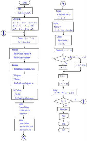
Figure 1.
Steepest descent also known as Powell’s method—flow diagram of Rankine cycle method used in this study.
This paper aims for a discussion and is presented mainly on technical viability considering the case for a commercial OTEC plant which could be installed in the sea areas of Kalumpang, Malaysia. The temperature in this sea area is used, and the case where the surface temperature changes is described thoroughly. The critical parameter for cost effectiveness, such as the cold seawater pipe length effect has been investigated. The OTEC plant performance analysis was conducted, and the results of a 10 MW OTEC plant using the Rankine cycle with heat exchangers of plate-type and NH3 as the working fluid are reported.
2. Analysis Method
2.1. OTEC Potential and Profile of Temperature
Temperatures of different sites were close to each other, as shown in Figure 2, which depicts the vertical temperature profile from Japan Oceanographic [18,19]. A closer examination of the sites reveals that there was a slight temperature change of 0.11 °C at each of the measured depths, with the tendency being greater in the areas shallower than 700 m deep. The temperature drops sharply from 27.5~28.5 °C at the surface to 7.2~7.5 °C at 600 m depth as the depth increases, and no distinct layer where warm seawater mixes layer to 600 m deep was observed, despite a notable change in temperature from the surface. After 600 m, the temperature of the seawater gradually dropped to 4.6 to 4.8 °C between 1050 m and 1150 m. As a result, a temperature difference of more than 20 degrees Celsius can be obtained in order to materialize a hybrid OTEC system in Sabah, Malaysia. An OTEC hybrid system generates both energy and water.
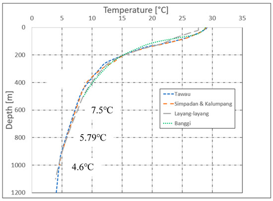
Figure 2.
Depth and deep seawater temperature profile of several potential sites in Sabah at 1000 m, 800 m, and 600 m, respectively. For simulation purpose, the applied data for Kalumpang was retrieved from Japan Oceanographic Data Center (JODC) (2020) 1000 m (4.6 °C), 800 m (5.79 °C), and 600 m (7.5 °C), respectively.
The temperature of the seawater is especially important in the design of an OTEC plant. A temperature difference of more than 20 °C between warm and cold seawater is required to establish a commercially viable OTEC plant. As a result, in this case, for a requirement of 5 °C cold seawater, the cold seawater pipe must be long enough to reach 900 m depth (as shown in the Figure 2).
2.2. Rankine Cycle
Figure 3 shows a schematic diagram of the Rankine cycle for an OTEC system. The basic equipment of the Rankine cycle is an evaporator, condenser, turbine, and working fluid pump. The principle of the OTEC system follows a continuous cycle of processes which starts with the working fluid circulation pump transporting the working fluid to the evaporator (3 → 4), and it vaporizes after the warm seawater exchanges the heat with it (4 → 1). Then, the vapor passes through the turbine and does the work (1 → 2). Followed by it, the working fluid enters the condenser after leaving the turbine, and exchange heat with the cold seawater before being condensed (2 → 3). The process continues, whereby the working fluid circulation pump returns the condensed working fluid to the evaporator for vaporization again (3 → 4) and these processes continue in OTEC closed cycle [20].
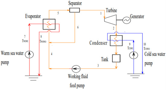
Figure 3.
The schematic diagram of OTEC cycle, where warm seawater is represented in red line, cold seawater in blue line and NH3, the working fluid in orange line.
Next, the Figure 4 shows the T-s diagram of the Rankine cycle which explains the significance of TE, and TC using NH3 as the working fluid. The efficiency of NH3 as the working fluid for the OTEC system was studied by Ganic and Wu (1980), and they found NH3 to be the best fluid owing to its highest thermal efficiency [21]. These were supported by several other studies in which, the latent heat of NH3 was found to be higher than halogenated hydrocarbons [22]. NH3 also outranked other types of working fluids in performance under a subcritical OTEC system [23].
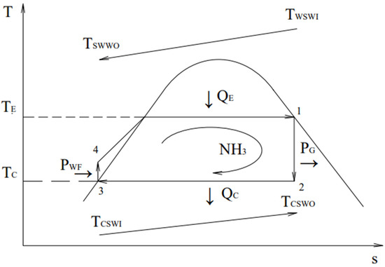
Figure 4.
T—s diagram of the Rankine cycle.
2.3. Objective Function
In the case of ocean thermal energy conversion, the cost required for power generation of the total cost (total cost) for use, and the cost of manufacturing the evaporator and condenser is approximately 30–50%. For this reason, minimizing the evaporator’s and condenser’s total surface area is considered to be the most critical factor in minimizing the total cost of power generation. Therefore, the objective function of the evaporator and condenser is defined and shown in Equation (1),
The value of γ is obtained by dividing the total heat transfer surface area AT with the net output PN (Net power) and is often used as the objective function for optimization [24,25]. It is clearly derived and identified in previous studies that the objective function γ, that is, the relationship between the total heat transfer area of the heat exchanger per (unit) 1 kW of output power and the inlet temperatures of warm and cold seawater, is important [26]. Therefore, the total heat transfer area of the heat exchanger in the objective function becomes small, and the net power output becomes large. As a result, the objective function becomes small (known as the minimum objective function) and the OTEC plant will be economically viable.
2.3.1. Net Power
The net power PN is defined as in Equation (2) [27,28],
PN = PG − (PWSW + PCSW + PWF)
PG in Equation (2) is the generated power, also known as gross power, PWSW is warm seawater pumping power, PCSW is cold seawater pumping power, and PWF is working fluid pumping power, shown in Equations (3)–(6).
where ∆PWSW is the total pressure difference between the warm seawater pipe and the cold seawater pipe, and ∆PCSW is the total pressure difference between the working fluid piping ∆PWF.
PG = mWF ηT ηG (h1 − h2)
∆PWSW is the total pressure variance of the warm seawater pipe, shown in Equation (7),
where the pressure difference in the evaporator is represented by ΔPWSWE, and ΔPWSWEA is the pressure difference around the evaporator.
∆PWSW = ΔPWSWE + ΔPWSWEA
ΔPWSWE is the pressure difference in the evaporator and is calculated as in Equation (8).
where ζE is the friction factor in the evaporator.
∆PWSWEA is assumed as 1.0 [m].
ΔPCSW is the total pressure difference of the cold seawater pipe, shown in Equation (9),
where ΔPCSWC is the pressure difference in the condenser, ΔPCSWCA is the pressure difference around the condenser, and ΔPCSWP is the pressure difference of the cold seawater piping.
ΔPCSW = ΔPCSWC + ΔPCSWCA +ΔPCSWP
ΔPCSWC is calculated as the pressure difference in the condenser as shown in Equation (10),
where ζC is the friction factor in the condenser.
ΔPCSWCA assumed it with 1.0 (m).
ΔPCSWP has calculated pressure is the pressure difference of the cold seawater piping as shown in Equation (11),
where ΔPCSWPf is the friction loss and ΔPCSWPD is the density difference of the cold seawater in the cold seawater piping, respectively.
ΔPCSWP = ΔPCSWPf + ΔPCSWPD
ΔPCSWPf is calculated using Equation (12) [29],
where CH = 100.
Next, ΔPCSWPD is calculated using Equation (13).
∆PWF is the total pressure difference of the working fluid piping, and is calculated using Equation (14),
where v1 = v3 is the specific volume in the condensing temperature TC, P1 the is evaporation pressure, P3 is the condensing pressure, and P0 is the pressure lost in working fluid piping (9.8 × 10⁴).
∆PWF = [v3 (P1 − P3)] + P0
2.3.2. Heat Transfer Area
The total heat transfer surface, AT, is given as in Equation (15) [30],
where AE and AC are the heat transfer area of the evaporator and condenser and are calculated using Equations (16)–(19).
where QE and QC are the evaporator and condenser heat transfer rates. The logarithmic mean temperature differences of the evaporator and condenser are (ΔTm)E and (ΔTm)C.
AT = AE + AC
The UE and UC represent the evaporator and condenser’s overall heat transfer coefficients, respectively. The heat transfer coefficient on warm sea water αWSW, the boiling heat transfer coefficient B, and the thermal conductivity of the heat transfer surface kWSW can be used to calculate UC. The heat transfer coefficient on cold seawater CSW, the condensation heat transfer coefficient C, and the thermal conductivity of the heat transfer surface αCSW can be used to calculate UC. In an OTEC system, the heat transfer area of the heat exchanger must be estimated.
Thus, calculations are carried out using the empirical equation which incorporates NH3 as the working fluid and plate-type evaporator to determine the boiling heat transfer coefficient. On the other hand, an empirical equation of a fluted plate was used for the heat transfer coefficient for condensation.
- (a)
- Boiling Heat Transfer Coefficient
The boiling heat transfer coefficient αB is calculated from the Equations (20) and (21) [31],
where,
M = 900 (m−1)
Pa = 1.976 (W)
- (b)
- Condensation Heat Transfer Coefficient
The condensation heat transfer coefficient of the working fluid αC and steam vapor in the desalination condenser αDC is calculated from the Equation (27) [32].
where,
- (c)
- Heat Transfer Coefficient of the Seawater side (Evaporator and Condenser)
The heat transfer coefficient of the seawater in the evaporator and condenser αWSW, αCSW and are calculated from Equation (34) [33].
where
2.4. Objective Function and Its Variables
Objective function γ in Equation (1) is dependent on various variables. There are five dependent variables that can be considered such as design condition variable C, shape factor G, state factor S, operation factor D, and piping factor P [25,33]. Among the variables, some experimental and empirical assumptions are incorporated to predict its values. Some variables are constant and some have upper and lower limits. Variables with upper limits include turbine efficiency, generator efficiency, and pump efficiency. Thus, upon limiting some variables, γ can be derived as Equation (37),
γ = f (TE, TC, VWSW, VCSW)
As shown in Equation (37), if the parameters of the generated power, working fluid, the material of the heat exchanger, an inlet temperature of warm seawater TWSW, and inlet temperature of the cold seawater TCSWI are given, γ is a function of the evaporation temperature TE, condensation temperature TC, warm seawater velocity in the evaporator VWSW and cold seawater velocity in the condenser VCSW. A minimum value of the objective function γmin can be calculated by the steepest descent or Powell’s method using Equations (2)–(36).
When optimizing the entire system, it is necessary to optimize each component. Therefore, the in-house program for optimizing these components was included as subroutines. In this study, REFPROP (Lemmon et al. (2013)), was used as the physical properties of anhydrous ammonia and seawater [34]. In addition, a Handbook (Society of Sea Water Science Japan, 1966), was used for the physical properties of warm and cold seawater [35].
Condition and Calculation Method
A flow chart of the method used in this study is developed as shown in the Figure 1. When optimizing the entire system, it is necessary to optimize each component. Therefore, the optimization program for these components is included as subroutines.
As shown in the Figure 1, first, calculate γ at a certain point. Next, fix other variables and calculate γ1 when one variable (for example TE) is slightly changed. Subsequently, the partial derivative for TE is obtained as (γ1 − γ)/ΔTE. Then, as a new initial value for TE, the step is multiplied by an arbitrary constant δ1 to proceed to the next step. Using the same method, TC, VWSW, and VCSW are obtained. As clearly shown in the Figure 1, γ is calculated using the new combination of variables to derive the minimum value of γ which is γmin.
Table 1 shows the design condition of the Rankine cycle OTEC plant which generates 10 MW of power. The length of the cold seawater pipes used in this calculation are 1000, 800, and 600 m, and its diameter is 5 m. From the perspective of the capital expenditure (CAPEX) of an OTEC plant, the shorter length of the cold seawater pipes would result in lowering the CAPEX. Thus, the length of cold seawater pipes must be thoroughly discussed and identified during the OTEC plant design and feasibility study phase.

Table 1.
Design conditions.
Anhydrous ammonia is used as the working fluid. Titanium being a strong and non-corrosive material is suitable for plate heat exchangers. The thermophysical properties of NH3 and the seawater are taken from [34,35], respectively. In this paper, optimization is carried out using the REFPROP as the thermophysical properties of NH3. In previous studies, PROPATH and other approximate values were used for NH3 which has resulted in a different optimization design.
3. Results and Discussion
3.1. Minimum Objective Function
Figure 5 shows the minimum value of the objective function versus the inlet temperature difference (TWSWI − TCSWI). The value of the minimum objective function is decreased when the inlet temperature difference (TWSWI − TCSWI) is increased as can be seen in the Figure 5. In other words, the objective function γ is smaller when the warm seawater inlet temperature, TWSWI is higher and the cold seawater inlet temperature, TCSWI is lower.
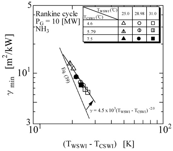
Figure 5.
Comparison of minimum objective function from Equation (38) (simulation from this study) and Equation (39) (comparing with empirical data from Uehara & Nakaoka, 1984)) [30].
For example, when TWSWI = 28.98 °C and TCSWI = 4.6 °C, γ = 7.44 m2/kW, whereas when TWSWI = 28.98 °C and TCSWI = 7.5 °C, γ = 9.14 m2/kW. Although the inlet temperature difference (TWSWI − TCSWI) under these two conditions is only 2.9 °C, the ratio of γ is 1:1.2 and significant. This indicates that the effect of cold seawater inlet temperature is large and impactful.
The objective function versus inlet temperature difference (TWSWI − TCSWI) is shown in Figure 5 and is given by Equation (38) in solid line:
γmin = 4.5 × 10³ (TWSWI − TCSWI)−2.0
The alternate dashed line in the Figure 5 is the result of a study on an OTEC system using a plate heat exchanger [30]. The system was calibrated and optimized for an output power of 100 MW. The minimum objective function obtained from that study is shown in Equation (39).
γmin = 1.3 × 10⁵ (TWSWI − TCSWI)−3.2
Comparing Equations (38) from this simulation study with (39) from [30], when TWSWI = 28.98 °C and TCSWI = 4.6 °C, γ = 7.44 m2/kW from Equation (38), whereas γ = 4.73 m2/kW from Equation (39), respectively. γ is about 1.57 times larger. The reason for this increase is probably due to the smaller power generation output of 10 MW. This is because when the power output decreases, the performance of the heat exchanger deteriorates and the total heat transfer area increases. Nevertheless, it could also be due to the efficiency of each component in the OTEC system (turbine, heat exchanger, pumps, and others) having improved and it caused an improvement in the total OTEC system, attributing an increase in the net power output.
As can be seen from Figure 5, even if TWSWI and TCSWI change, considering within the range of (TWSWI − TCSWI), the objective function γ is determined only by the temperature difference between warm and cold seawater inlets. Performance analysis for the OTEC system must be done considering the minimum objective function for cost viability.
3.2. Pumping Power and Net Power
Figure 6a–c show the net power PN, the warm seawater pumping power PWSW, the cold seawater pumping power PCSW and the working fluid pumping power PWF versus the inlet temperature difference (TWSWI − TCSWI). In the Figure 6a–c, cold seawater pipe length is 1000 m, 800 m, and 600 m, respectively.
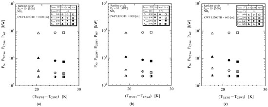
Figure 6.
(a–c) Net power and pumping power.
The values of warm seawater pumping power and cold seawater pumping power decrease when the inlet temperature difference (TWSWI − TCSWI) is increased as can be seen in the Figure 6a–c. The working fluid pumping power is constant when an inlet temperature difference is increased. The working fluid pumping power is estimated to be 200 kW.
Because the pumping power of the warm seawater and cold seawater decreases when the inlet temperature difference (TWSWI − TCSWI) is increased, the value of the net power is increased when the inlet temperature difference (TWSWI − TCSWI) is increased as can be seen in the Figure 6a–c.
Observing the effect of the length of cold seawater pipe, the net power is greater with 1000 m of cold seawater pipe than with 600 m. This is because the net power is larger when the temperature of the cold seawater is lower. In addition, it is said that when the cold seawater temperature becomes low, both, the cold seawater flow rate and pump power decrease, respectively.
3.3. Warm and Cold Seawater Flow Rate
Figure 7a–c shows the warm and cold seawater flow rate versus the inlet temperature difference. In Figure 7a–c, cold seawater pipe length is 1000 m, 800 m, and 600 m, respectively. The warm and cold seawater flow rate decreases as the inlet temperature difference increases. Because the heat transfer area of the evaporator and condenser decrease when the inlet temperature difference (TWSWI − TCSWI) is increased, the warm and cold sea water flow rate are decreased when the inlet temperature difference (TWSWI − TCSWI) is increased as can be seen in Figure 7a–c.
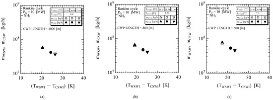
Figure 7.
(a–c) Flow rate of warm and cold seawater.
Further analysis by considering cold seawater pipe lengths for 1000 m and 600 m is performed. In the case of 1000 m, TWSWI = 28.98 °C and TCSWI = 4.6 °C, warm seawater flow rate mWSW = 4.321 × 10⁷ kg/h, cold seawater flow rate mCSW = 4.151 × 10⁷ kg/h, respectively. On the other hand, in the case of 600 m, TWSWI = 28.98 °C and TCSWI = 7.5 °C, warm seawater flow rate mWSW = 5.216 × 10⁷ kg/h and cold seawater flow rate mCSW = 5.364 × 10⁷ kg/h, respectively. An observation was made that the warm seawater flow rate mWSW ratio of 1000 m is smaller than 600 m at 1:1.2 and the cold seawater flow rate mCSW ratio of 1000 m is also smaller than 600 m at 1:1.3, respectively.
3.4. Heat Transfer Area
Figure 8a–c shows the total heat transfer area AT, the heat transfer area of the evaporator AE, and the heat transfer area of the condenser AC versus the inlet temperature difference. In the Figure 8a–c, cold seawater pipe length is 1000 m, 800 m, and 600 m, respectively.
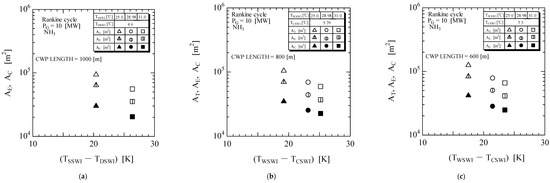
Figure 8.
(a–c) Heat transfer area.
The value of the total heat transfer area, the heat transfer area of the evaporator, and the heat transfer area of the condenser decreased when the inlet temperature difference (TWSWI − TCSWI) is increased as can be confirmed in Figure 8a–c.
This is because the heat transfer coefficient of the evaporator and condenser is increased when the inlet temperature difference (TWSWI − TCSWI) is increased, and the heat transfer area of the evaporator and condenser is decreased when the inlet temperature difference (TWSWI − TCSWI) is increased as can be seen in the Figure 8a–c.
Further analysis of AT by considering cold seawater pipe lengths as 1000 m and 600 m is performed. In the case of 1000 m, TWSWI = 28.98 °C and TCSWI = 4.6 °C, the total heat transfer area AT = 6.446 × 10⁵ m2. On the other end, in the case of 600 m, TWSWI = 28.98 °C and TCSWI = 7.5 °C, the total heat transfer area AT = 7.812 × 10⁵ m2. It was observed that the total heat transfer area AT ratio of 1000 m is smaller than 600 m at 1:1.2.
Nevertheless, if the empirical equation of other types of heat exchangers is known, the heat transfer coefficient can be used in the optimization calculation using a similar method as discussed in this paper.
4. Feasible OTEC Plant Specification
The OTEC design is determined based on the site location and power requirements. There are three different designs to accommodate all scenarios: submersible type, floating, and land based. Hence, this paper will be mainly on technical viability considering the case for a commercial OTEC plant which could be installed in the sea areas off Sabah, namely Kalumpang, as this is one of the strategic sites for an on-land commercial OTEC plant in Malaysia.
Previous reports have shown the temperature distribution in other sea areas and the optimal OTEC system design by [36,37]. Thus, it was found that the optimum objective function, pump power, flow rate, and heat exchanger area are dependent on the temperature difference between warm and cold seawater inlet temperature (TWSWI − TCSWI). As a result, it is possible to estimate the total OTEC system output if the warm seawater inlet temperature TWSWI and the cold seawater inlet temperature TCSWI are known from surveys of other sea areas.
The OTEC plant proposed for Malaysia is with a gross-power of 10 MW floating type. A conceptual idea in Figure 9 shows a floating type OTEC power plant. In this OTEC power plant, the monitoring area and control room are above the seawater surface. All of the OTEC plant components are enclosed in a pressured containment designed below the seawater surface.
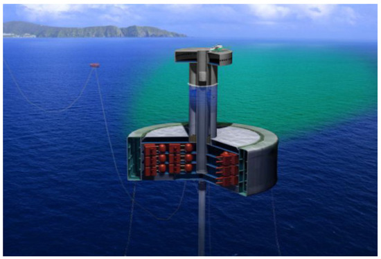
Figure 9.
A conceptual idea of the floating-type OTEC [38].
5. Conclusions
In this paper, the performance analysis of a commercial OTEC plant was carried out at a potential site in Sabah, Malaysia. Incorporating various Kalumpang’s oceanographic data of WSW and CSW, the design of a 10 MW OTEC plant using the Rankine cycle and anhydrous ammonia as the working fluid and plate type heat exchangers has been proposed.
The results of numerical analysis from this simulation are compared with those of the Rankine cycle (Equations (38) and (39) (Uehara & Nakaoka, 1984)) and the following results were obtained [30]:
- The value of the minimum objective function is decreased when the inlet temperature difference (TWSWI − TCSWI) is increased as can be seen in the Figure 5 (comparison between Equations (38) and (39)). Pertaining to this value, the minimum objective function versus the inlet temperature difference was derived and shown in Equation (38). Comparing 10 MW and 100 MW, the objective function of 10 MW is larger, resulting in a higher CAPEX.
- The value of the warm seawater pumping power and cold seawater pumping power is decreased when the inlet temperature difference (TWSWI − TCSWI) is increased.
- Even if the inlet temperature difference is increased, the working fluid pumping power is constant. The working fluid pumping power is as small as 200 kW.
- Because the pumping power of the warm seawater and cold seawater decreases when the inlet temperature difference (TWSWI − TCSWI) is increased, the value of the net power is increased when the inlet temperature difference (TWSWI − TCSWI) is increased.
- The warm and cold sea water flow rate decreases as the inlet temperature difference increases.
- The value of the total heat transfer area, the heat transfer area of the evaporator, and the heat transfer area of the condenser decreased when the inlet temperature difference (TWSWI − TCSWI) is increased.
Future projects could include hybrid-OTEC optimization for 2.5 or 10 MW commercial plants as a solution for carbon net-zero. Another possible extension of these findings would be the development of an economically viable OTEC Malaysian Model.
Author Contributions
Conceptualization, T.Y. and H.K.; Methodology, S.T.T., H.J.K., T.Y. and T.N.; Software, A.A.A.; Validation, S.T.T., A.B.J., S.R., T.N. and H.K.; Formal analysis, S.R., H.J.K. and S.C.; Investigation, A.A.A., H.K. and S.C.; Resources, S.T.T. and Y.I.; Data curation, S.R., T.N. and Y.I.; Writing—original draft, S.T.T.; Writing—review & editing, T.N., S.T.T., H.K. and Y.I. All authors have read and agreed to the published version of the manuscript.
Funding
This research was funded by Japan Science and Technology (JST, JPMJSA1803) and Japan International Cooperation Agency (JICA) and the Ministry of Higher Education (MoHE) of Malaysia for MyPAIR SATREPS OTEC grant with Vote number R.K130000.7856.4L894 and UTM Matching Grant, Q.K130000.3056.04M21 and Q.K130000.2656.15J80 (RUG Grant Tier 2).
Institutional Review Board Statement
Not applicable.
Informed Consent Statement
Not applicable.
Data Availability Statement
Not applicable.
Acknowledgments
The authors are grateful to acknowledge the Science and Technology Research Partnership for Sustainable Development (SATREPS) funded by Japan Science and Technology (JST, JPMJSA1803) and Japan International Cooperation Agency (JICA) and the Ministry of Higher Education (MoHE) of Malaysia for MyPAIR SATREPS OTEC grant with Vote number R.K130000.7856.4L894 and UTM Matching Grant, Q.K130000.3056.04M21 and Q.K130000.2656.15J80 (RUG Grant Tier 2). The authors sincere appreciation to Tetsuya Nishida and their team from the National Fisheries University, Japan for their efforts in validating and support on bathymetry and maps of Sabah, Malaysia.
Conflicts of Interest
The authors declare no conflict of interest.
Nomenclature
| A | heat transfer area | (m2) |
| Bo | Bond number | (-) |
| Bo* | modified Bond number | (-) |
| cp | specific heat at constant pressure | (kJ/kgK) |
| d | diameter | (m) |
| Deq | equivalent diameter | (m) |
| fp | pressure factor | (-) |
| g | gravitational acceleration | (m/s2) |
| Gr | Grashof number | (-) |
| h | enthalpy | (kJ/kg) |
| depth of flute | (m) | |
| H | ratio of sensible to latent heat | (-) |
| k | thermal conductivity | (W/mK) |
| l | length | (m) |
| L | latent heat | (kJ/kg) |
| ∆L | width of plate | (m) |
| m | mass flow rate | (kg/s) |
| Nu | Nusselt number | (-) |
| P | Power | (W) |
| Pressure | (Pa) | |
| Pr | Prandtl number | (-) |
| Prop | property | (-) |
| ΔP | pressure difference | (Pa) |
| q | heat flux | (W/m2) |
| Q | heat flow rate | (kJ) |
| Re | Reynolds number | (-) |
| t | thickness of plate | (mm) |
| T | temperature | (°C) |
| ∆T | temperature difference | (°C) |
| ∆Tm | logarithmic temperature difference | (°C) |
| U | overall heat transfer coefficient | (W/m2K) |
| v | specific volume | (m3/kg) |
| V | velocity | (m/s) |
| X | non-dimensional number | (-) |
| ∆X | length of plate | (m) |
| Y | non-dimensional number | (-) |
| ∆Y | clearance of plate | (m) |
| α | heat transfer coefficient | (W/m2K) |
| γ | objective function | (m2/kW) |
| ζ | friction factor | (-) |
| η | efficiency | (-) |
| υ | dynamic viscosity | (Pa s) |
| ν | kinematic viscosity | (m2/s) |
| ρ | density | (kg/m3) |
| σ | surface tension | (N/m) |
| Subscripts | ||
| a | atmosphere | |
| B | boiling | |
| C | condenser | |
| CSW | cold seawater | |
| D | density | |
| E | evaporator | |
| f | friction loss | |
| G | generator | |
| I | inlet | |
| L | length | |
| L | liquid | |
| m | mean | |
| min | minimum | |
| N | net | |
| O | outlet | |
| T | turbine | |
| V | vapor | |
| W | wall | |
| WF | working fluid | |
| WSW | warm seawater | |
References
- ASEAN Centre for Energy. ASEAN Energy Database System. 2019. Available online: https://aeds.aseanenergy.org/country/malaysia/ (accessed on 25 April 2020).
- Abdullah, A.H.; Ridha, S.; Mohshim, D.F.; Yusuf, M.; Kamyab, H.; Krishna, S.; Maoinser, M.A. A comprehensive review of nanoparticles in water-based drilling fluids on wellbore stability. Chemosphere 2022, 308, 136274. [Google Scholar] [CrossRef] [PubMed]
- Uehara, H.; Dilao, C.O.; Nakaoka, T. Conceptual Design of Ocean Thermal Energy Conversion (OTEC) Power Plants in the Philippines. Sol. Energy 1988, 41, 431–441. [Google Scholar] [CrossRef]
- Hashim, H.; Zubir, M.A.; Kamyab, H.; Zahran, M.F.I. Decarbonisation of the Industrial Sector Through Greenhouse Gas Mitigation, Offset, and Emission Trading Schemes. Chem. Eng. Trans. 2022, 97, 511–516. [Google Scholar]
- Nihous, G.C. An estimate of Atlantic Ocean thermal energy conversion (OTEC) resources. Ocean Eng. 2007, 34, 2210–2221. [Google Scholar] [CrossRef]
- Langer, J.; Quist, J.; Blok, K. Upscaling scenarios for ocean thermal energy conversion with technological learning in Indonesia and their global relevance. Renew. Sustain. Energy Rev. 2022, 158, 112086. [Google Scholar] [CrossRef]
- Arcuri, N.; Bruno, R.; Bevilacqua, P. LNG as cold heat source in OTEC systems. Ocean Eng. 2015, 104, 349–358. [Google Scholar] [CrossRef]
- Martin, B.; Okamura, S.; Nakamura, Y.; Yasunaga, T.; Ikegami, Y. Status of the “Kumejima Model” for advanced deep seawater utilization. In Proceedings of the 2016 Techno-Ocean (Techno-Ocean 2016), Kobe, Japan, 6–8 October 2016; pp. 211–216. [Google Scholar]
- Seungtaek, L.; Hosaeng, L.; Junghyun, M.; Hyeonju, K. Simulation data of regional economic analysis of OTEC for applicable area. Processes 2020, 8, 1107. [Google Scholar] [CrossRef]
- Langer, J.; Cahyaningwidi, A.A.; Chalkiadakis, C.; Quist, J.; Hoes, O.; Blok, K. Plant siting and economic potential of ocean thermal energy conversion in Indonesia a novel GIS-based methodology. Energy 2021, 224, 120121. [Google Scholar] [CrossRef]
- Langer, J.; Quist, J.; Blok, K. Recent progress in the economics of ocean thermal energy conversion: Critical review and research agenda. Renew. Sustain. Energy Rev. 2020, 130, 109960. [Google Scholar] [CrossRef]
- Adiputra, R.; Utsunomiya, T.; Koto, J.; Yasunaga, T.; Ikegami, Y. Preliminary design of a 100 MW-net ocean thermal energy conversion (OTEC) power plant study case: Mentawai Island, Indonesia. J. Mar. Sci. Technol. 2019, 25, 48–68. [Google Scholar] [CrossRef]
- Martel, L.; Smith, P.; Rizea, S.; Van Ryzin, J.; Morgan, C.; Noland, G.; Pavlosky, R.; Thomas, M.; Halkyard, J. Ocean Thermal Energy Conversion Life Cycle Cost Assessment; Final Technical Report; Lockheed Martin: Manassas, VA, USA, 30 May 2012. [Google Scholar]
- Yeh, R.-H.; Su, T.-Z.; Yang, M.-S. Maximum output of an OTEC power plant. Ocean Eng. 2005, 32, 685–700. [Google Scholar] [CrossRef]
- Bernardoni, C.; Binotti, M.; Giostri, A. Techno-economic analysis of closed OTEC cycles for power generation. Renew. Energy 2018, 132, 1018–1033. [Google Scholar] [CrossRef]
- Uehara, H.; Ikegami, Y. Optimization of a closed-cycle OTEC system. J. Sol. Energy Eng. 1990, 112, 247–256. [Google Scholar] [CrossRef]
- Giostri, A.; Romei, A.; Binotti, M. Off-design performance of closed OTEC cycles for power generation. Renew. Energy 2021, 170, 1353–1366. [Google Scholar] [CrossRef]
- Thirugnana, S.; Jaafar, A.B.; Yasunaga, T.; Nakaoka, T.; Ikegami, Y.; Su, S. Estimation of Ocean Thermal Energy Conversion Resources in the East of Malaysia. J. Mar. Sci. Eng. 2021, 9, 22. [Google Scholar] [CrossRef]
- Japan Oceanographic Data Center. 2020. Available online: https://www.jodc.go.jp/jodcweb/ (accessed on 20 April 2020).
- Ikegami, Y.; Yasunaga, T.; Morisaki, T. Ocean thermal energy conversion using double-stage Rankine cycle. J. Mar. Sci. Eng. 2018, 6, 21. [Google Scholar] [CrossRef]
- Ganic, E.; Wu, J. On the selection of working fluids for OTEC power plants. Energy Convers. Manag. 1980, 20, 9–22. [Google Scholar] [CrossRef]
- Stoecker, W.F. Comparison of ammonia with other refrigerants for district cooling plant chillers. ASHRAE Trans. Am. Soc. Heat. Refrig. Airconditioning Engine 1994, 100, 1126–1135. [Google Scholar]
- Kim, N.; Shin, S.; Chun, W. A study on the thermodynamic cycle of OTEC system. J. Korean Sol. Energy Soc. 2006, 26, 9–18. [Google Scholar]
- Uehara, H.; Nakaoka, T.; Monde, M.; Yamashita, T. Study of ocean thermal energy conversion using double fluted Tube (1st report, in case of NH3 as working fluid). Trans. Jpn. Soc. Mech. Eng. 1983, 49, 1214–1223. (In Japanese) [Google Scholar] [CrossRef]
- Uehara, H.; Nakaoka, T.; Isogai, H.; Misago, T.; Jitsuhara, S. Optimization of ocean thermal energy conversion plant consisting of shell and plate type heat exchanger. In Proceedings of the JSME/PSME Joint Conference; The American Society of Mechanical Engineers: New York, NY, USA, 1987–2010; pp. 1–20. [Google Scholar]
- Uehara, H.; Nakaoka, T. Study of ocean thermal energy conversion using plate type heat exchanger (in case of NH3 as working fluid). Trans. Jpn. Soc. Mech. Eng. 1984–1988, 50, 1955–1962. (In Japanese) [Google Scholar] [CrossRef]
- Uehara, H.; Nakaoka, T. Study of ocean thermal energy conversion system using of the plate type heat exchanger. JSME 1984, 50, 1955–1962. (In Japanese) [Google Scholar] [CrossRef]
- Uehara, H.; Nakaoka, T. Ocean thermal energy conversion plant for small island. Proc. Eng. 1987–1993, 2, 1029–1034. [Google Scholar]
- JSME. Fluid Resistance in Pipe and Duct. Japan. In JSME Data Book; JSME: Kyoto, Japan, 1983. (In Japanese) [Google Scholar]
- Uehara, H.; Nakaoka, T.; Hagiwara, K. Plate type condenser (cold water side heat transfer coefficient and friction factor). Refrigeration 1984, 59, 3–9. (In Japanese) [Google Scholar]
- Nakaoka, T.; Uehara, H. Performance test of a shell-and-plate type evaporator for OTEC. Exp. Therm. Fluid Sci. 1988, 1, 283–291. [Google Scholar] [CrossRef]
- Uehara, H.; Nakaoka, T.; Nakashima, S. Heat transfer coefficients for a vertical fluted-plate condenser with R113 and R114. Int. J. Refrig. 1985, 8, 22–28. [Google Scholar] [CrossRef]
- Uehara, H.; Nakaoka, T. Study of ocean thermal energy conversion using plate type heat exchanger (in case of R22 as working fluid). Trans. Jpn. Soc. Mech. Eng. 1984–1985, 50, 1325–1333. (In Japanese) [Google Scholar] [CrossRef]
- Lemmon, E.W.; Huber, M.L.; McLinden, M.O. REFPROP, NIST Standard Reference Database 23, v. 9.1; National Institute of Standards: Gaithersburg, MD, USA, 2013. [Google Scholar]
- Society of Sea Water Science Japan. Handbook of Using Sea Water; Society of Sea Water Science Japan: Tokyo, Japan, 1966; p. 108. (In Japanese)
- Ikegami, Y.; Urata, K.; Fukumiya, K.; Noda, N.; Decherong, G. Oceanographic Observation in the Palau waters for utilization of cold deep seawater. In Proceedings of the 6th Conference at Kumejima Session of Japan Association of Deep Ocean Water Applications, Seoul, Republic of Korea, 19–24 June 2002; p. 27. [Google Scholar]
- Nakaoka, T.; Nishida, T.; Ichinose, J.; Nagatomo, K.; Mizutani, S.; Tatsumi, S.; Matsushita, M.; Pickering, T.; Ikegami, Y.; Uehara, H. Oceanographic observations and an estimate of the renewable energy for ocean thermal energy conversion in the coast of the Fiji Island. Deep Ocean Water Res. 2003, 4, 57–66. [Google Scholar]
- Xenesys Inc. Ocean Thermal Energy Conversion. 2022. Available online: http://www.xenesys.com/products/otec.html (accessed on 3 February 2022). (In Japanese).


Disclaimer/Publisher’s Note: The statements, opinions and data contained in all publications are solely those of the individual author(s) and contributor(s) and not of MDPI and/or the editor(s). MDPI and/or the editor(s) disclaim responsibility for any injury to people or property resulting from any ideas, methods, instructions or products referred to in the content. |
© 2023 by the authors. Licensee MDPI, Basel, Switzerland. This article is an open access article distributed under the terms and conditions of the Creative Commons Attribution (CC BY) license (https://creativecommons.org/licenses/by/4.0/).