Article

Innovative Dynamic Queue-Length Estimation Using Google Maps Color-Code Data

by
Promporn Sornsoongnern
,
Suthatip Pueboobpaphan
and
Rattaphol Pueboobpaphan
*
School of Transportation Engineering, Institute of Engineering, Suranaree University of Technology, Nakhon Ratchasima 30000, Thailand
*
Author to whom correspondence should be addressed.
Sustainability 2023, 15(4), 3466; https://doi.org/10.3390/su15043466
Submission received: 30 December 2022 / Revised: 1 February 2023 / Accepted: 8 February 2023 / Published: 14 February 2023
(This article belongs to the Topic Intelligent Transportation Systems)

Abstract

:
Queue length is an important parameter for traffic-signal priority systems for emergency vehicles. Instead of using conventional detector data, this paper investigates the feasibility of queue-length estimation using Google Maps color-code data via random forest (RF) and gradient-boosting machine (GBM) methods. Alternative ways of specifying independent variables from color-code data are also investigated. Additionally, the models are separated by peak or off-peak periods and by the presence or absence of adjacent upstream signalized intersections. The results show that the performance predicted by the RF and GBM methods is similar in all cases. Although the error values of both methods are relatively high, they are considerably lower than those obtained from estimates using historical queue-length data. The results obtained using variable-importance analysis show that the importance of the red band near an intersection is significantly higher than that of other variables for a direction without a prior signalized intersection. For a direction with a prior signalized intersection, the importance varies, depending on the period (peak or off-peak). Since Google Maps data are available and cover most of the world intersections, the proposed approach provides a cost-effective option for cities with no detectors installed.

1. Introduction

Traffic signaling is an effective way of managing traffic at intersections by reducing the conflict points and keeping the traffic through intersections in order. All vehicles must compulsorily stop at a red traffic light; this, unavoidably, causes traffic delays. However, for emergency vehicles, reducing the delays caused by red-light stops by just a few seconds is essential when the lives of patients are in danger. Current traffic-signal priority systems can detect and assign priority to emergency vehicles at signalized intersections [1,2,3,4]. An important parameter in such a system is the length of the vehicle queue at that intersection and at that time. This parameter is used to analyze the optimal timing interval required to activate the green signal in advance and to clear the queue from the intersection before emergency vehicles arrive.
In most studies, data from detectors employing the shockwave theory have been used to estimate queue lengths at signalized intersections. Recent studies have attempted to improve the efficiency of queue-length estimation by focusing on the aspects of real time and high accuracy. Queue-length data can also be used to adjust traffic signals and manage traffic congestion [5,6,7,8,9]. However, in almost every intersection in Thailand, no detectors have yet been installed. Therefore, in practice, it is not possible to estimate the queue length using this method. With this limitation in mind, Jodnok and Pueboobpaphan [10] applied linear regression analysis and random forest (RF) analysis to estimate the queue length at signalized intersections during peak and off-peak periods using color-code traffic data obtained from Google Maps. The results showed that the queue-length estimation using these data was sufficient to some extent, and the RF method exhibited lower errors than those exhibited by other methods.
Many researchers have used Google Maps data in their studies. Travel time and distance data from Google Maps were used to determine the optimal location for installing a charging station [11]. The data were also used to determine the traffic volume and vehicle speed to investigate road congestion [12,13], air pollution [14,15], or accessibility to hospitals [16]. Travel-route data from Google Maps were also used to route cargo and emergency vehicles [17,18,19]. Color-code and travel-time data from Google Maps were used to adjust the traffic-signal timings in response to near-real-time traffic conditions [20]. The color-code data were also used to forecast traffic conditions for urban roads using historical averages [21]. Traffic-speed data from Google Maps were used to determine the congestion index [22]. However, there is a lack of research on using color-code data from Google Maps to estimate the queue length at signalized intersections.
Google Maps display four possible colors: dark red, red, orange, and green. These colors represent traffic conditions according to vehicle speed, ranging from very low to high speed [23,24]. Jodnok [25] observed color codes by capturing Google Maps screenshots around a signalized intersection every 1 min. He found that the dark red and red bands appeared less frequently than other bands, leading to the question of whether these two colors should be considered, as they had the same color in the model.
Some works have reported the use of the RF technique in various areas of transportation research [26,27,28]. However, other machine-learning techniques besides RF have also been applied. For instance, the gradient-boosting machine (GBM) technique has been applied when the relationship between dependent and independent variables is nonlinear. GBM applications include travel-time prediction [29], incident-clearance-time prediction [30], and short-term traffic-volume prediction [31]. The GBM technique was found to provide better predictions than other methods [30,31]. Moreover, new studies have shown that the GBM method can calculate the variable importance (VI), which helps understand how important each independent variable is to a dependent variable. This is an added advantage of the GBM method, which was previously considered a black-box method, because of its ability to provide better information about the relationships between dependent and independent variables compared with other methods [32].
This paper extends the study by Jodnok and Pueboobpaphan [10]. In addition to peak/off-peak periods, we consider modeling, which is based on directions with or without an upstream signalized intersection in the vicinity. Furthermore, we consider alternative ways of modeling independent variables using color-code traffic data. Specifically, we consider dark red and red as being the same color and green as a reference color. The predicted results obtained using the RF and GBM methods are compared with those estimated by the historical averages, and VI analysis is performed to understand the factors affecting the prediction of queue length using color codes from Google Maps. The objective is to assess the feasibility and limitations of developing a method for estimating the queue length from the color-code traffic data obtained from Google Maps. This method will provide an alternative for those areas where no detectors are installed at signalized intersections on a road network.
In the next section, the data collection and survey are briefly explained. Details of how color-code data from Google Maps and actual queue-length data from the field were collected and processed as independent and dependent variables, respectively, are described. Details on modeling scenarios are then provided, followed by modeling results and the variable importance (VI) analysis. The conclusions and recommendations complete the paper.

2. Materials and Methods

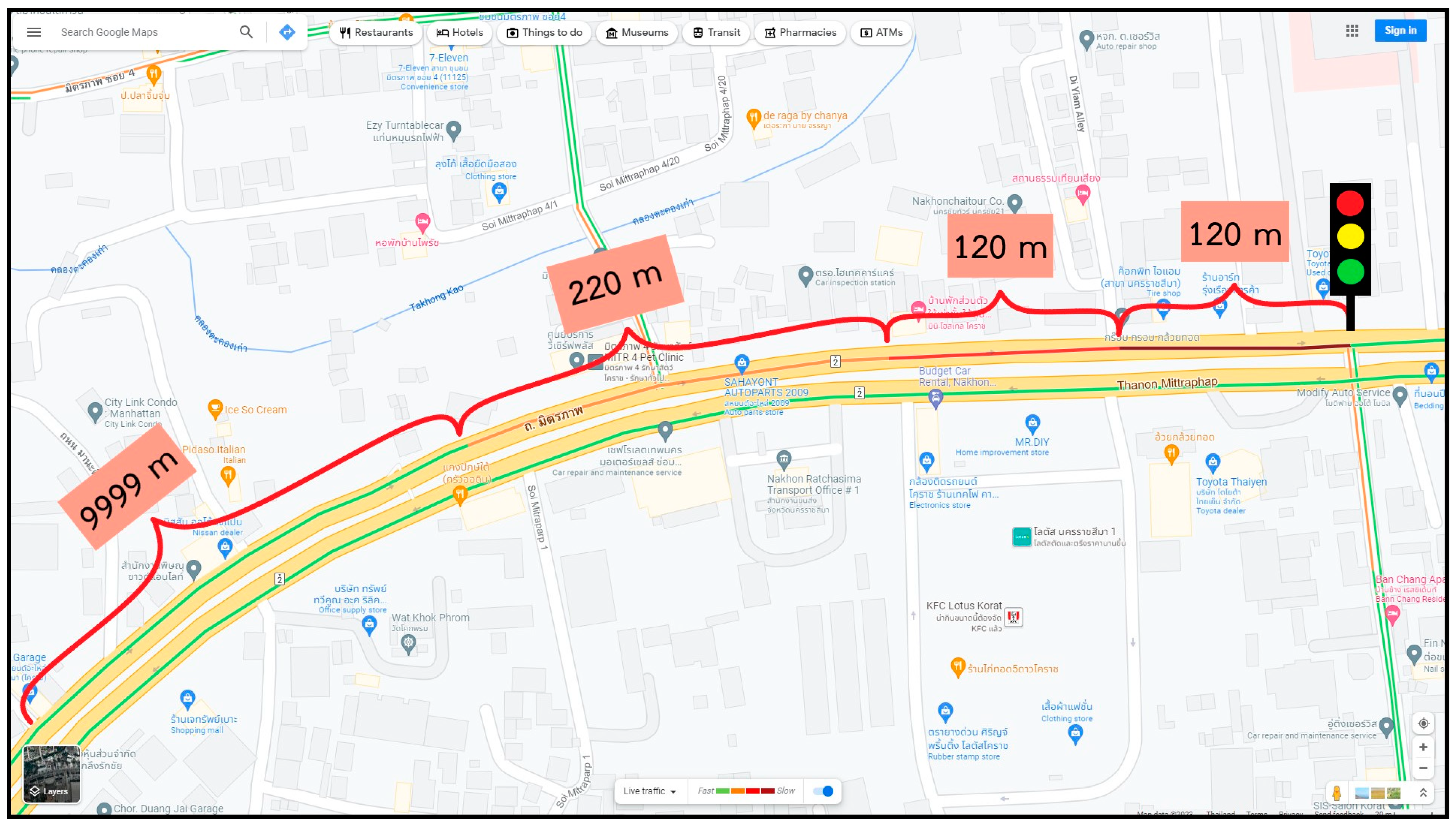
This paper uses the same data as those used by Jodnok and Pueboobpaphan [10], who surveyed and collected data of colors and lengths of each consecutive color band from Google Maps. They also simultaneously recorded the actual queue lengths. The area of study was a T-signalized intersection on the main arterial road in the Nakhon Ratchasima province, Thailand. The intersection is located in an area with heavy traffic and frequent traffic jams. There are four lanes in each direction. Figure 1 shows the area of study, where a prior traffic signal is absent in the inbound direction, but present in the outbound direction at a distance of 930 m upstream from the studied intersection. The survey and data collection was started at 7:00 a.m. and completed at 7:00 p.m. to cover the peak and off-peak periods. The survey was conducted for three days during weekdays and for two days during weekends.

2.1. Collection of Color-Code Data from Google Maps

A screenshot of Google Maps, which covers the entire area of investigation, was captured every 1 min. The Google Maps website was continually refreshed using the Auto-Refresh program to illustrate the change in the color-code data continuously. It was observed that in the direction without a prior signalized intersection, the last band shown on the edge of the screen was always a green-color band. Figure 2 shows an example of the color-code data obtained from Google Maps, where four color bands are displayed; the 1st band from the stop line is dark red with a length of 120 m, followed by a 120 m red band, a 220 m orange band, and finally, a green band, which extends beyond the screen. The length of the last band was specified as 9999 m. An example of the data extraction from the Google Maps screenshot (shown in Figure 2) is presented in Table 1.

2.2. Survey of the Actual Queue-Length Data

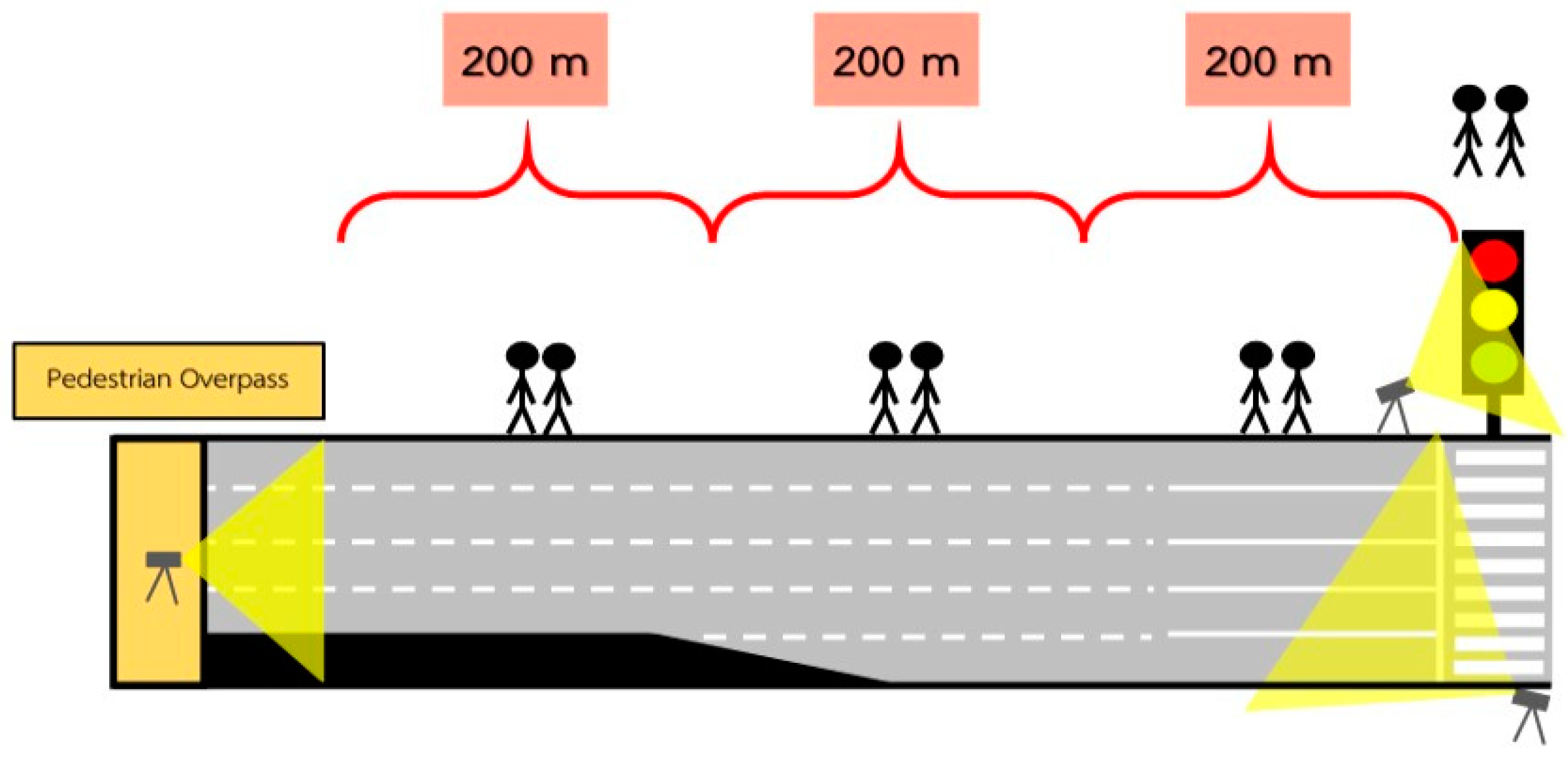
The actual queue lengths were surveyed by observers in the field. The curb was temporarily marked with a reflective tape every 20 m from the stop line. These marks were viewed against the tails of the queuing vehicles for measuring the queue length. In addition, a detailed map indicating the distance to various landmarks, such as buildings, light poles, billboards, and other structures that can be easily seen from a distance, was prepared to assist the observers in measuring the queue lengths. Generally, the queue lengths of the lanes may not be the same, but in our case, they are not much different. Therefore, the average of the queue lengths obtained from all four lanes was used to represent the queue length that was used as a dependent variable in the model. Seven fourth-year undergraduate students and one graduate student from the School of Transportation Engineering, Suranaree University of Technology, were recruited for field observation. Every two students had to cover a 200 m segment for two different lanes. Six students, thus, covered a total distance of 600 m of a four-lane road segment, which was sufficient in our case study. The remaining two students had to stand-by at the site for replacing their friends while also monitoring video cameras used to record traffic volume and traffic signals. The observers used radio communication to communicate about the current position of the queue tail. They were asked to follow the queue tail, if it is in the segment for which they were responsible, to record the actual queue length every 1 min (the same interval of capturing as the Google Maps screen). A speed threshold of less than 10 km/h was used to identify approaching vehicles as being in the queue. The direction and time were also recorded to identify whether the queue length was observed during peak or off-peak periods and whether there was a prior signalized intersection. When all vehicles were moving during the green signal and no queue occurred, the queue length was recorded as zero. Figure 3 illustrates the distribution of the observers and video cameras in the study area. Note that the inbound and outbound directions were observed independently on different days.

2.3. Data Processing

Jodnok and Pueboobpaphan [10] found that the highest number of bands counting from the stop line was six on the surveyed road section. The color bands were defined so that the band closest to the intersection was assigned as the first band, and the band furthest from the intersection was assigned as the last band. They also found that using data from the first three bands adjacent to the stop line was sufficient and produced equivalent performance to that of using data from all six bands. Therefore, in this paper, data from only the first three bands adjacent to the stop line were used to create independent variables. In addition, the following alternative ways of processing color-code data as independent variables were attempted:
Independent variable set 1 (IV1): consider all four original colors of Google Maps as in [10].
Independent variable set 2 (IV2): consider dark red and red as if they were the same color.
Independent variable set 3 (IV3): similar to IV2, but the green variable is also considered as a reference color and is dropped.
The name of the independent variables used in the model is shown in Table 2. The recorded value of each independent variable depends on whether the actual color from Google Maps matches the color of the variable as indicated by Equation (1). If the actual color of band i is the same color as the variable j_i, then the length of band i in meters is recorded. Otherwise, variable j_i will be zero.
j _ i = { l e n g t h   o f   b a n d   i ,   i f   a c t u a l   c o l o r   o f   b a n d   i   i s   j   0 ,   o t h e r w i s e

2.4. Modeling

In this paper, two machine-learning techniques, namely, the RF and GBM, are applied. The RF is an ensemble decision-tree method. The principle of RF is to create multiple decision trees, where each employs the same algorithm, but has different features. The data used to construct each tree are randomly selected from the same database. When a decision tree is completed, the data are returned to the original database, and a new set of data is randomly selected to create a new decision tree [33]. The GBM technique is an improved technique based on the RF technique. GBM is considered an ensemble learning technique. Initially, GBM creates a weak classifier and then calculates the error values. GBM learns the pattern of error values, improves to reduce the error, and builds a new model. Thus, the error in the new model is less than that of the previous one. GBM continues the modeling sequentially, until the error cannot be learned. Then, model building is stopped [34].
In addition to the RF and GBM techniques, a simple estimation method is considered in this paper. This method uses the average of historical queue lengths, which are separated by the direction and by the period, as the estimate of the queue length in each case. This is later called the Average method. It represents the simplest possible estimation, which does not require any other input, except for the historical queue-length data. The results obtained using the Average method were used as a benchmark for comparison with the results obtained from the RF and GBM methods.
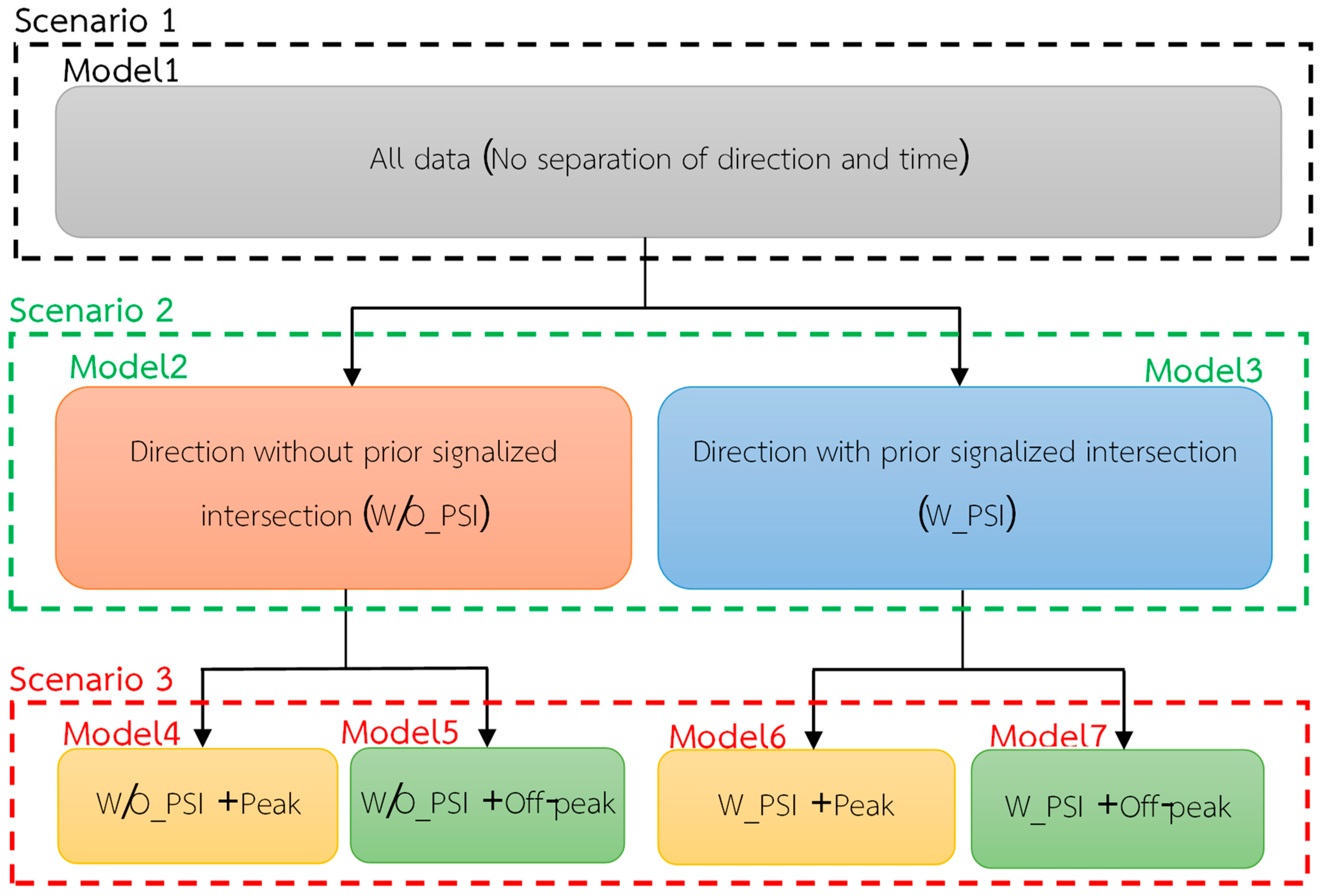
In general, traffic and queue patterns may differ between directions with and without a prior signalized intersection as well as between peak and off-peak periods. In this paper, seven different models based on these factors are considered. These models are described below and illustrated in Figure 4.
Model 1 (M1): Model with no separation of the direction and period
Model 2 (M2): Model for a direction without a prior signalized intersection and no separation of the period
Model 3 (M3): Model for a direction with a prior signalized intersection and no separation of the period
Model 4 (M4): Model for a direction without a prior signalized intersection and a peak period
Model 5 (M5): Model for a direction without a prior signalized intersection and an off-peak period
Model 6 (M6): Model for a direction with a prior signalized intersection and a peak period
Model 7 (M7): Model for a direction with a prior signalized intersection and an off-peak period
Based on the models described above, the following three equivalent scenarios were considered in the queue-length estimation:
Scenario 1: Model 1 was used to predict queue lengths in all cases with no separation of the direction and period.
Scenario 2: Model 2 was used to predict the queue length in a direction without a prior signalized intersection, and Model 3 was used to predict the queue length in a direction with a prior signalized intersection.
Scenario 3: Models 4 and 5 were used to predict queue lengths in a direction without a prior signalized intersection during peak and off-peak periods, respectively. Models 6 and 7 were used to predict queue lengths in a direction with a prior signalized intersection during peak and off-peak periods, respectively.
In this paper, the queue-length estimation models were constructed using RF and GBM from the packages in R [35], namely, caret [36] and gbm [37], respectively. To perform RF modeling using the caret package, the cforest method was used, and the tuning parameter of this method, mtry, which is the number of randomly selected predictors, was tuned in the 3–12 range. In GBM, caret was also used for parameter tuning. The GBM parameters were n.trees, interaction.depth, shrinkage, and n.minobsinnode. The entire dataset was divided into two subsets. The first 90% of data were used for training and modeling using a five-fold cross-validation method. The remaining 10% of data were used to test the prediction performance based on the root mean square error (RMSE) and the mean absolute percentage error (MAPE).
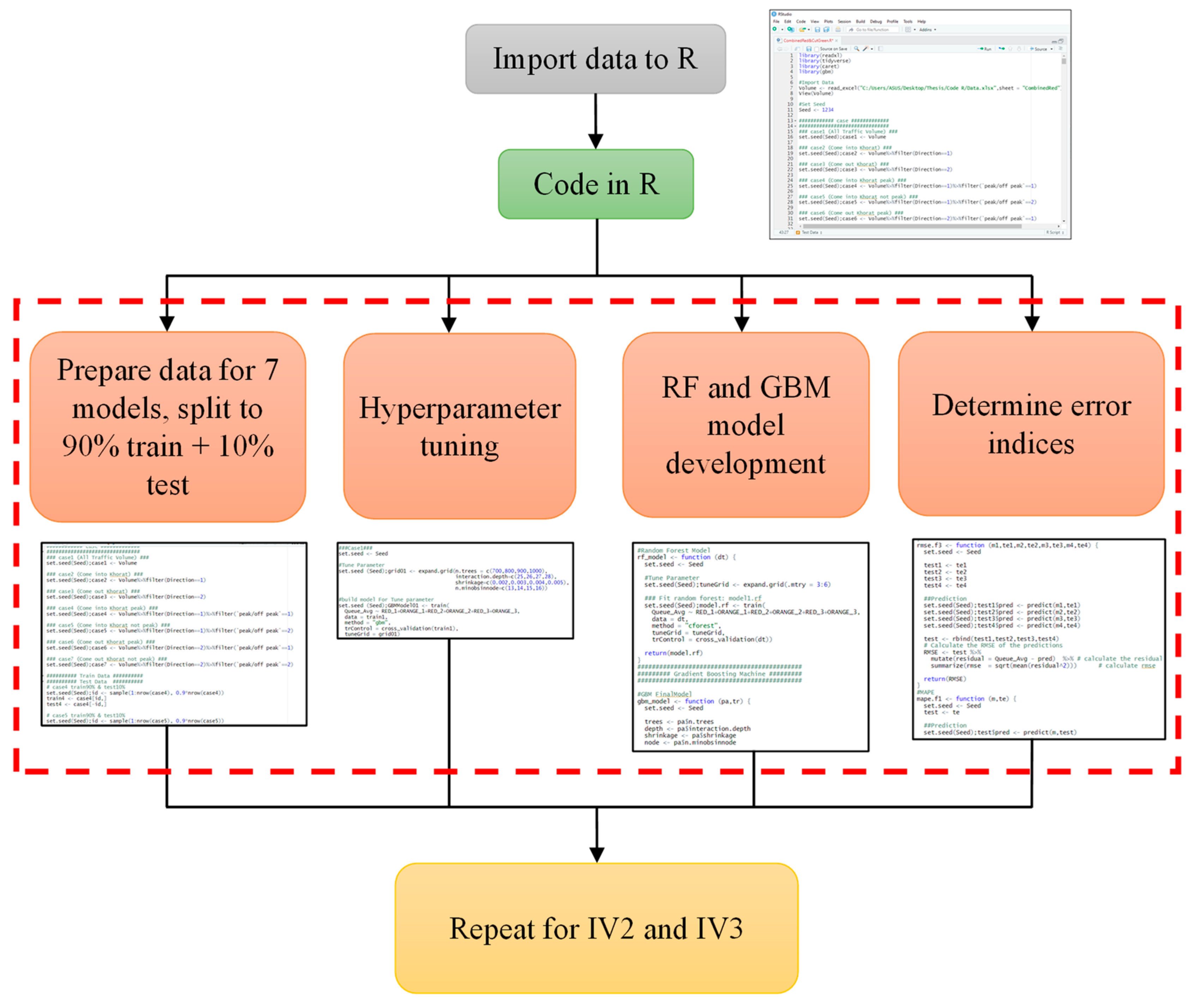
Figure 5 shows the overall modeling and analysis procedures. The procedures are summarized as follows:
1. Import actual queue length and color-code length data into the R program.
2. Create a separate dataset for each of the seven models.
3. Divide each dataset into 90% for training and 10% for testing.
4. For each of the independent variable sets, the training dataset is used for tuning the hyperparameters of the models. The GBM method uses package caret to tune the parameters. There are four parameters to tune: n.trees, interaction.depth, shrinkage, and n.minobsinnode. At first, a wide range of the parameter values were used for tuning. Subsequently, it is adjusted to a narrower range to fine-tune and seek the best value.
5. Once the optimum parameters are obtained, the GBM model is developed using the gbm package so that VI analysis can be performed. For the RF method, parameter tuning and modeling are performed simultaneously by the caret package.
6. The developed models are applied to the test dataset to predict the queue length, compare it with the actual queue length, and determine the error indices (RMSE and MAPE).
7. Repeat step 4–6 for other sets of independent variables.

3. Results and Discussion

3.1. Performance of the Queue-Length Estimation Models

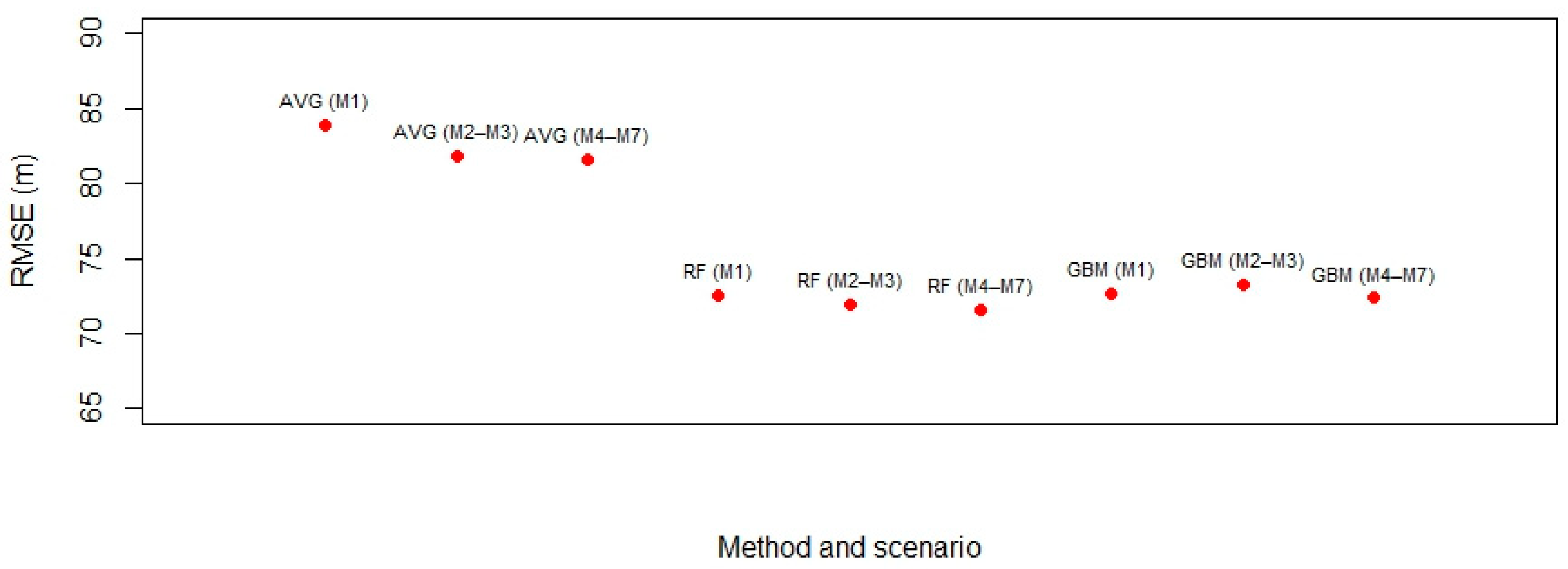
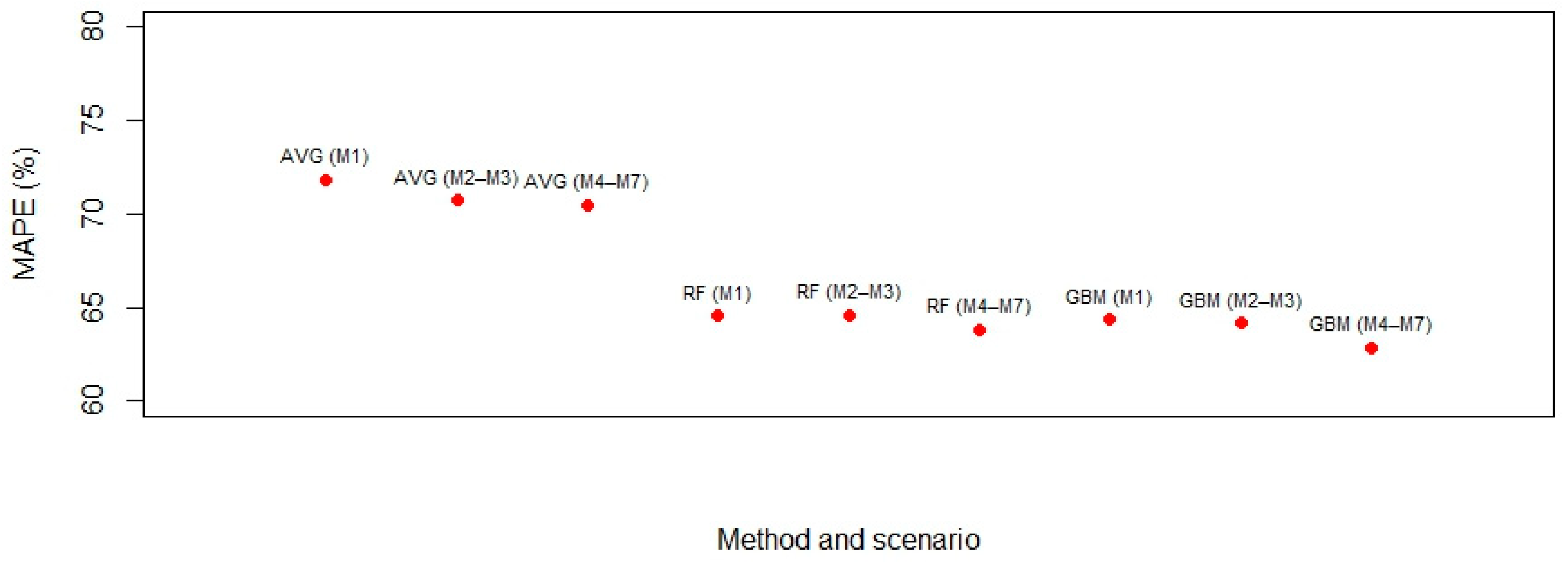
The prediction performances of the queue-length estimation models obtained from color-code data using the RF, GBM, and Average methods are presented and compared. Table 3 shows the RMSE and MAPE from all three scenarios and three sets of independent variables, whereas Figure 6 and Figure 7 show only the values from IV3 of each scenario and method. The results show that the lowest values of RMSE and MAPE are obtained in Scenario 3 with IV3 (combined red; green is used as a reference) using the RF and GBM methods, respectively. However, when comparing the RMSE and MAPE values in Scenario 3 vs. those in Scenarios 1 and 2, or IV3 vs. IV1 and IV2, no significant difference is observed. The error values are quite similar in all scenarios and all sets of the independent variables. Therefore, it is not possible to clearly discuss the differences between the RF and GBM methods. Nevertheless, the RMSE and MAPE values in both methods are significantly lower than those obtained using the Average method in all cases.
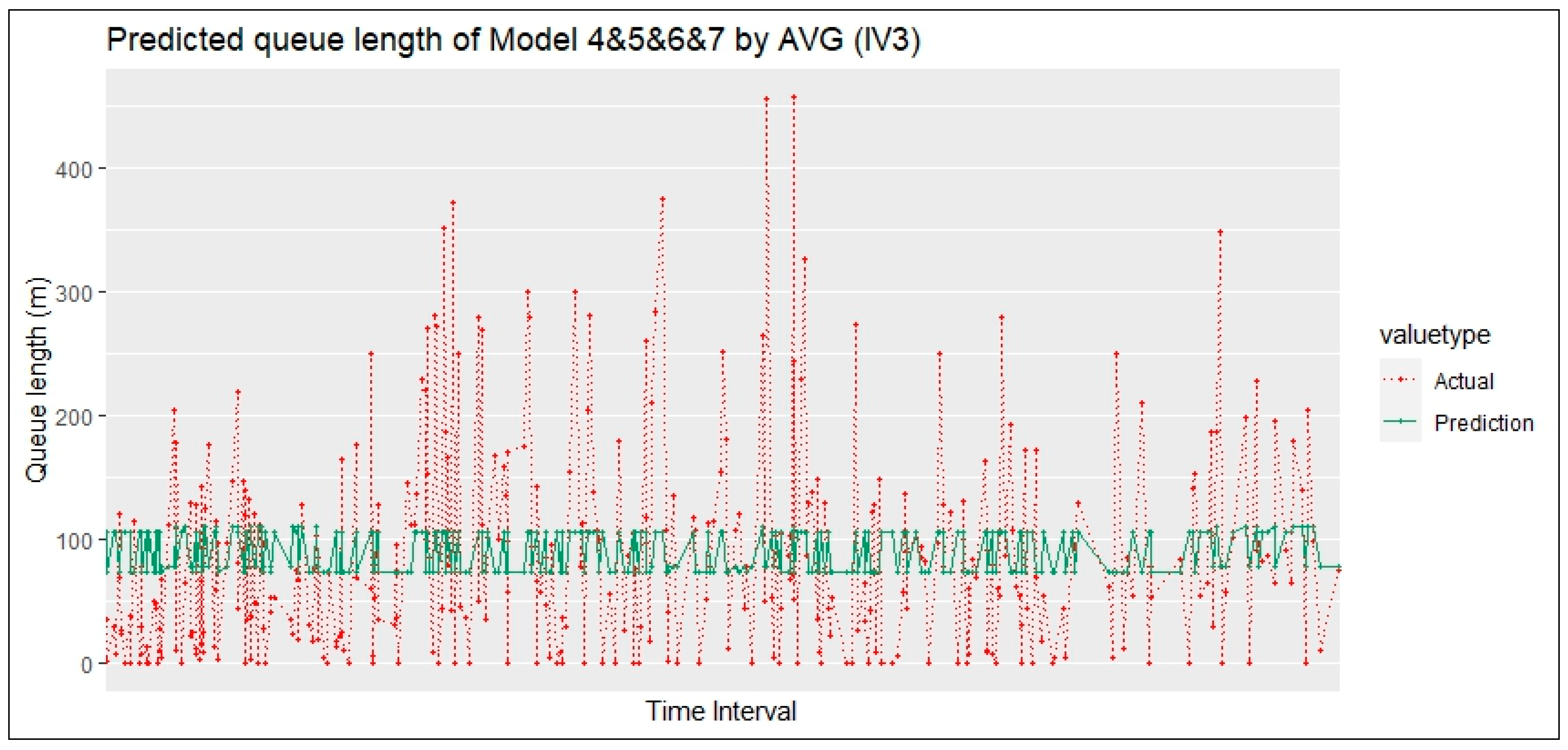
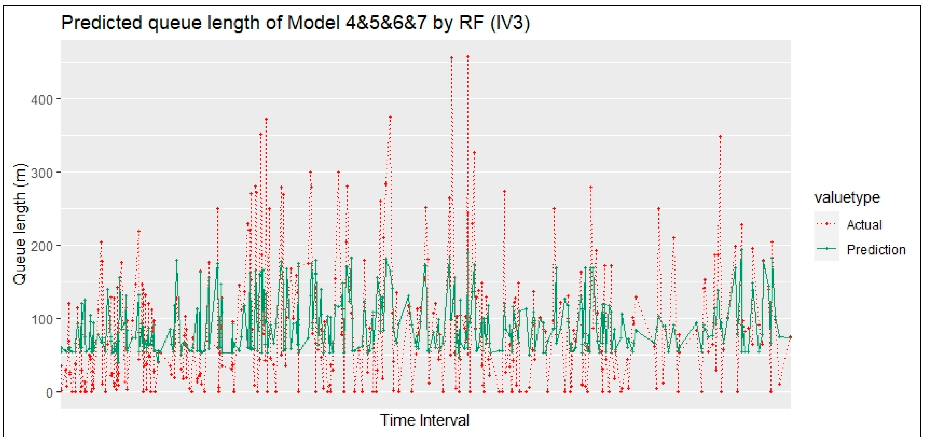
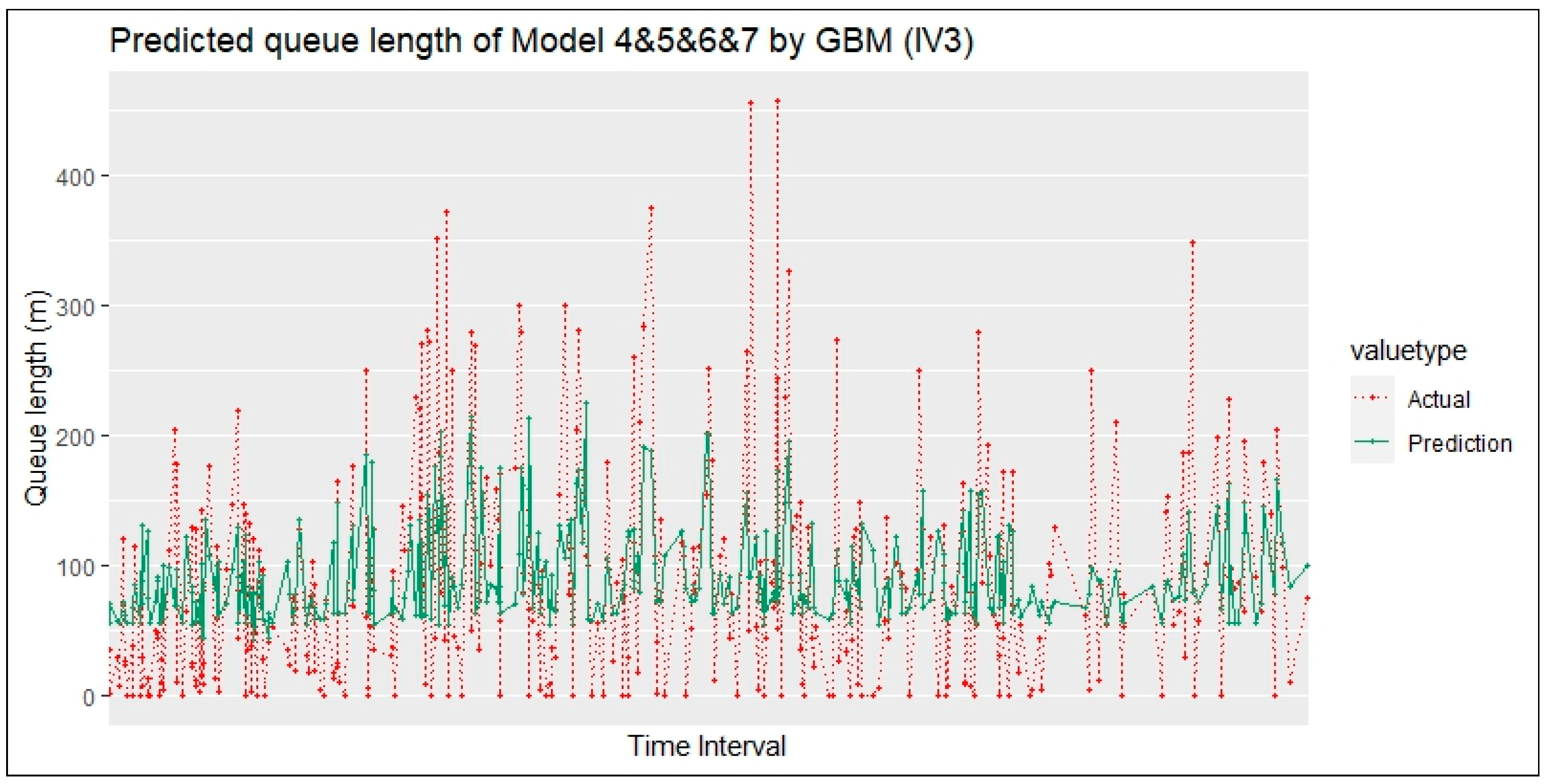
The above table shows that the queue-length predictions obtained using the RF and GBM methods are significantly better than those obtained using the Average method. Figure 8, Figure 9 and Figure 10 show the actual queue lengths obtained from the test dataset against the predicted queue lengths obtained using different methods in Scenario 3 with IV3. Although the predicted lengths obtained using the Average method can vary slightly depending on the direction and period, they cannot follow the dynamic change of the actual queue lengths. On the other hand, the lengths obtained using the RF and GBM methods can sufficiently follow the dynamic change of the actual queue lengths. Although the values obtained from both models still differ considerably from the actual values, their ability to capture the variations of the actual queue length is significantly better than that of the Average method.
It is worth noting that the traffic data from Google Maps is historical data based on previous measurements. The use of these data for traffic control, particularly with priority, may be debatable, as control at any given time must be adapted to the current length of the queue. Based on the prediction accuracy shown in Table 3 and Figure 8, Figure 9 and Figure 10, the proposed approach might not be sufficient for control operation, but it might be useful for design purposes, such as determining the length of additional lanes to turn at an intersection.

3.2. Variable Importance (VI) Analysis

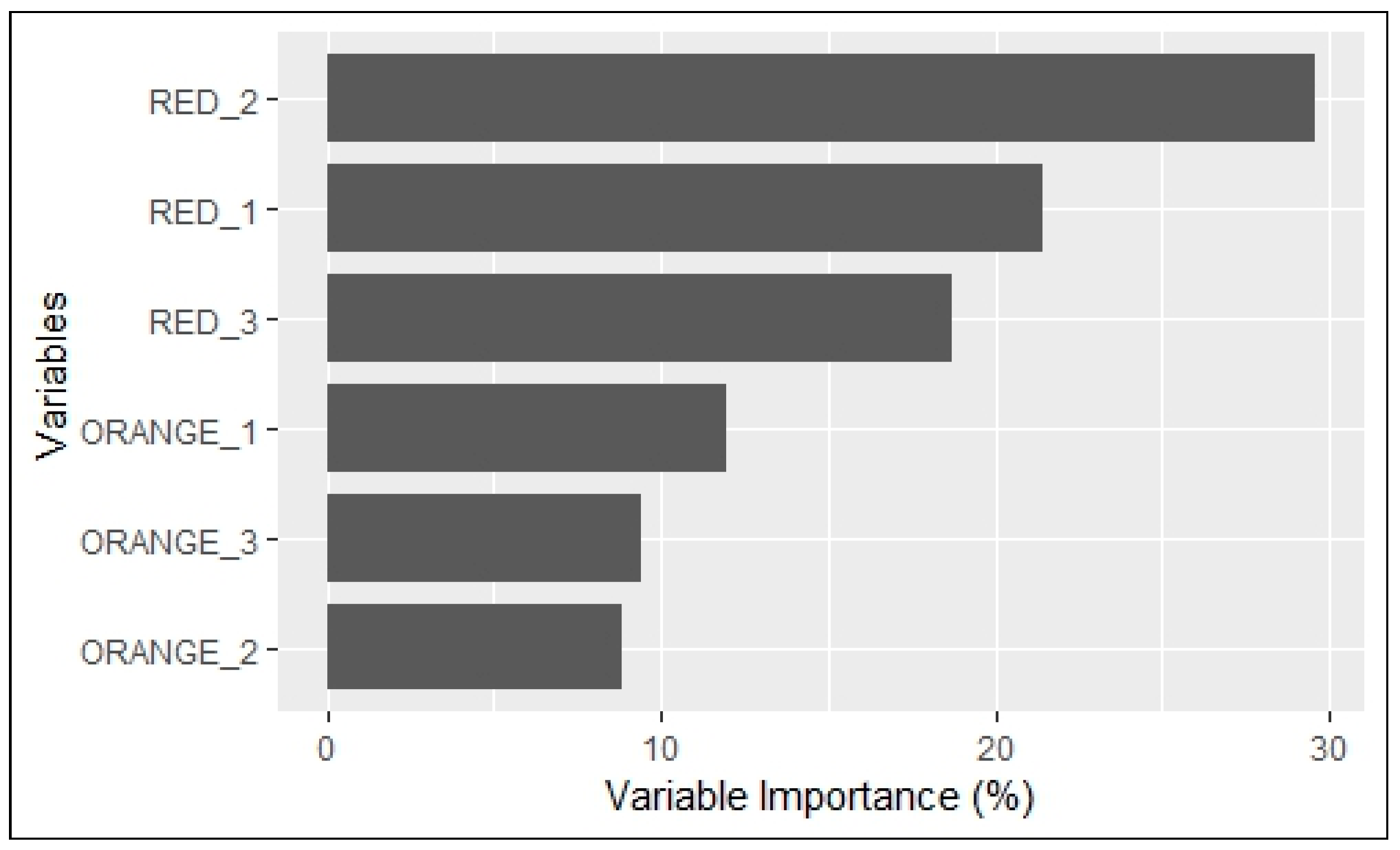
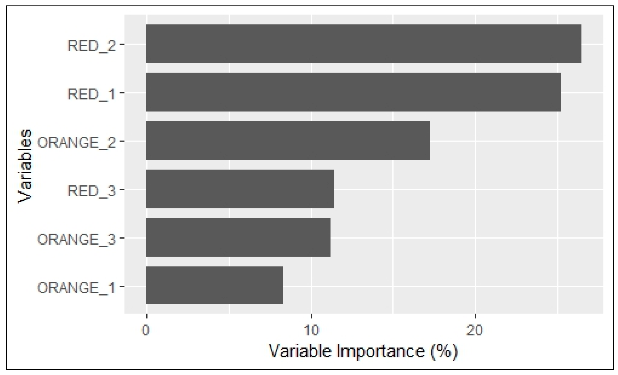
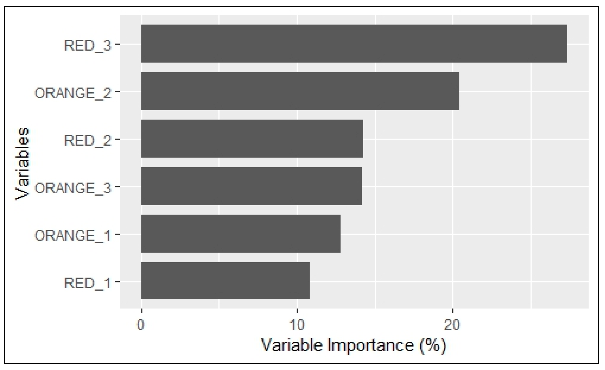
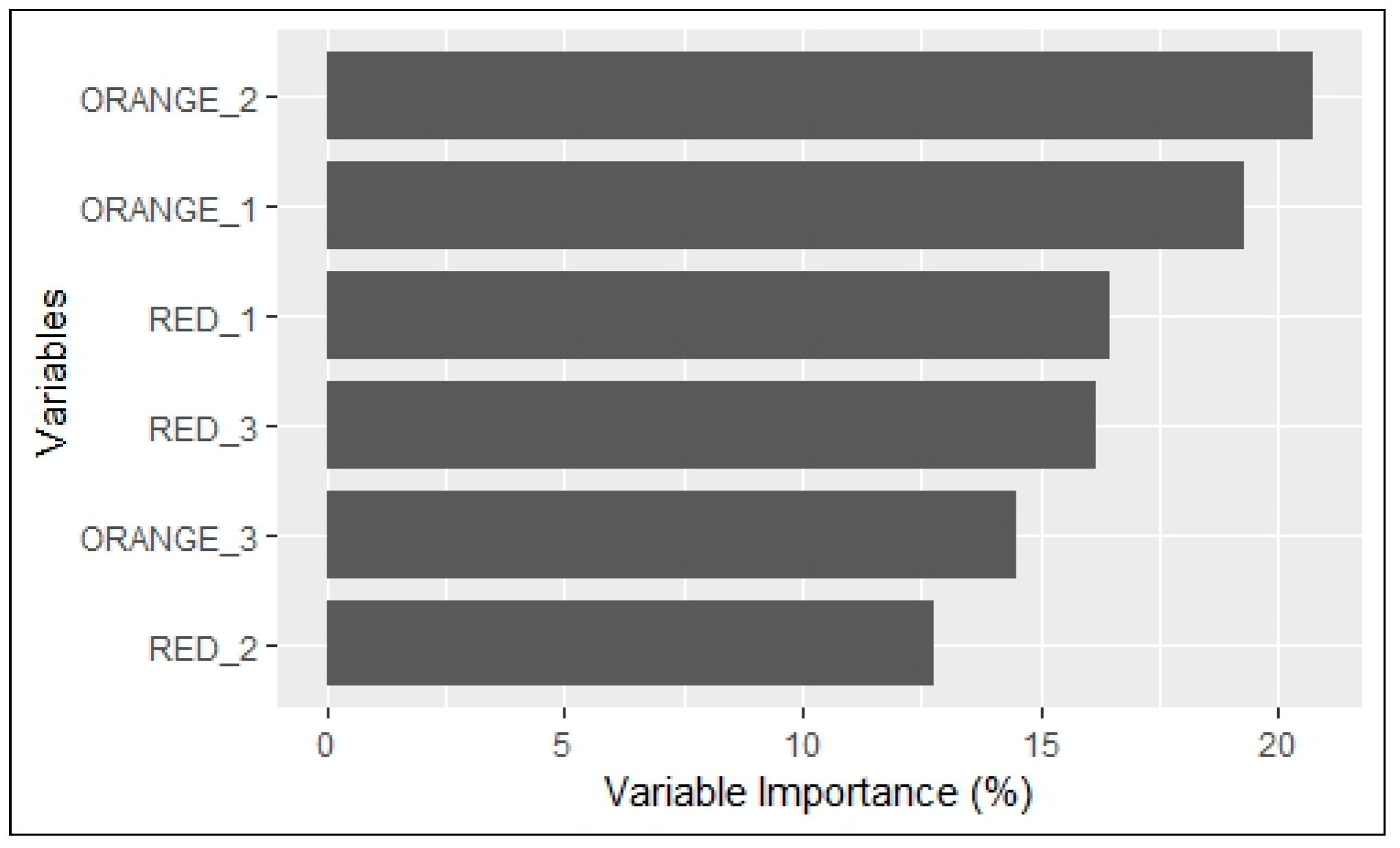
To better understand how the importance of the color band and its length affect the queue length and whether this importance differs between cases, the variable importance (VI) analysis results obtained using the GBM method in Scenario 3 (Models 4–7) with IV3 are presented. A variable with a high VI value is considered very important and highly affects the queue-length estimation. The VI analysis results (in percentage and in descending order) for each model are shown in Table 4 and Figure 11, Figure 12, Figure 13 and Figure 14.
The VI analysis results for Models 4 and 5, which correspond to the cases for a direction without a prior signalized intersection, show that the importance of the red band near the intersection is significantly higher than that of the other variables. The first two variables with the highest VI values are C_RED_2 and C_RED_1. During peak hours (Model 4), the importance level of the most important variable is significantly different from that of the second most important variable (29.61% for C_RED_2 vs. 21.45% for C_RED_1). This is different from the off-peak period, where the importance level of the most important variable is not significantly different from that of the second most important variable (26.47% for C_RED_2 vs. 25.22% for C_RED_1).
Comparisons between peak and off-peak periods for the direction with a prior signalized intersection (Models 6 and 7, respectively), indicate similar and different trends to those for the direction without a prior signalized intersection (Models 4 and 5). Regarding the same trends, during peak hours, the importance level of the most important variable is significantly different from that of the second most important variable (27.39% for C_RED_3 vs. 20.46% for ORANGE_2). During off-peak hours, the importance level of the most important variable is not significantly different from that of the second most important variable (20.75% for ORANGE_2 vs. 19.29% of ORANGE_1). Especially in Model 7, the importance level of each variable is not much different. This implies that the model can only partly capture the dynamic change of the actual queue lengths. However, the trend that differs from the direction without a prior signalized intersection is in the order of the variables, where C_RED_2 and C_RED_1 are no longer the top two most important variables. C_RED_3 and ORANGE_2 or ORANGE_1 are the most important variables in this case. This may be due to the updating and displaying of the Google Maps traffic color-code data, which are not real-time data, causing the traffic color-code display on Google Maps to be inconsistent with the actual queue length obtained from the survey. In addition, there is a difference in the distribution pattern of the arriving vehicles when a prior signalized intersection is absent or present. The arrival process for the direction without a prior signalized intersection is random, where vehicles arrive regularly, as opposed to the cluster-like pattern for the direction with a prior signalized intersection, where vehicles arrive in a platoon during the green, alternating with gaps during the red of the prior signal. With such characteristics, the traffic and queue for the direction with a prior signalized intersection are expected to show a relatively higher variation than that for the direction without a prior signalized intersection. As a result, the Google Maps color-code data in the direction with a prior signalized intersection may not be able to reflect well the changes in the traffic queue compared to those in the direction without a prior signalized intersection.

4. Conclusions

The objective of this paper was the estimation of traffic-queue lengths at signalized intersections using a new data source, specifically traffic color-code data obtained from Google Maps. The RF and GBM methods were employed and compared with a simple estimation method that uses only historical average queue-length data (i.e., the Average method). The original color-code data were processed to construct three different alternatives of independent variable specifications: (i) considering the colors as actually displayed on Google Maps, (ii) considering the dark red and red as if they were the same color, and (iii) using the green as a reference color. This study showed that the RF and GBM methods achieve similar prediction performance in all scenarios and provide independent variable specifications. Also, they perform significantly better than the Average method.
The VI analysis for a direction without a prior signalized intersection showed that the importance of the red band near the intersection is significantly higher than that of other variables. For a direction with a prior signalized intersection, the importance varies, depending on the period (peak or off-peak period), and the red band near the intersection is no longer the most important parameter. The off-peak period model showed that the importance of the color-code variable is not very different among all variables. The order of color bands based on their importance also differs between the two directions. This may be due to the updating frequency of the Google Maps data, which are not displayed in real time, causing the color-code data displayed on Google Maps to be inconsistent with the actual queue length obtained from the survey. Such non-real-time updates along with the cluster-like vehicle arrival pattern for a direction with a prior signalized intersection, cannot capture the relatively high dynamic changes in the traffic and the actual queue lengths. Thus, it is difficult for the model to capture information from the color-code data to estimate the queue length.
This study is a starting point for the feasibility of estimating queue lengths using color-code data obtained from Google Maps and provides an alternative to conventional approaches that use detector data. The proposed approach was able to estimate the queue length well only to a certain extent. Although the error of the proposed approach is still relatively high, it is far better than the error obtained using only historical queue-length data. This error can be attributed to several reasons, especially the non-real-time update of Google Maps. In addition, the display resolution of the Google Maps color bands, where the lengths are often displayed in a hierarchical order, may also affect the estimation of the queue length. Future research direction will be to investigate if the prediction accuracy of real-time queue-length estimation can be further increased by providing internet data processing technologies with additional capabilities such as the real-time display of color-code information and a better display resolution of color-band lengths. Other machine-learning techniques, such as neural network, support vector machines, and deep learning, will be adopted and compared to improve prediction accuracy. Another area of focus is to investigate and estimate the delay time of Google Maps updates, and develop methods to incorporate such delay time into the estimation procedure.

Author Contributions

Conceptualization, R.P. and S.P.; methodology, R.P. and P.S.; software, R.P. and P.S.; validation, R.P., P.S. and S.P.; formal analysis, R.P. and P.S.; investigation, R.P. and P.S.; data curation, P.S.; writing—original draft preparation, R.P. and P.S.; writing—review and editing, R.P., P.S. and S.P.; visualization, P.S.; supervision, R.P.; project administration, S.P. All authors have read and agreed to the published version of the manuscript.

Funding

This research received no external funding.

Institutional Review Board Statement

Not applicable.

Informed Consent Statement

Not applicable.

Data Availability Statement

Not applicable.

Conflicts of Interest

The authors declare no conflict of interest.

References

  1. Venkat, G.; Arulananth, T.S.; Baskar, M. Density Based Traffic Controller with Emergency Override using CCTV Camera. Int. J. Recent Technol. Eng. 2019, 8, 866–869. [Google Scholar] [CrossRef]
  2. Chuo, H.; Seah, Y.; Tan, K.; Lim, K.; Liau, C.; Kin Teo, K. On-Demand Priority Traffic Optimizer with Fuzzy Logic Microcontroller. In Proceedings of the 2022 IEEE International Conference on Artificial Intelligence in Engineering and Technology (IICAIET), Kota Kinabalu, Malaysia, 13–15 September 2022; pp. 1–6. [Google Scholar]
  3. Agarwal, H.; Rai, J. Traffic Control System Based on Density with Emergency Priority Mechanism. In Proceedings of the 2022 International Conference on Electronics and Renewable Systems (ICEARS), Tuticorin, India, 16–18 March 2022; pp. 192–197. [Google Scholar]
  4. Vishnu, U.; Sarma, S.; Yashumithaa, M.; Kr, S.; Gv, V. CNN Based Intelligent Traffic Control System to Support Emergency Vehicles. In Proceedings of the 2022 IEEE International Conference on Electronics, Computing and Communication Technologies (CONECCT), Bangalore, India, 8–10 July 2022; pp. 1–5. [Google Scholar]
  5. Lee, S.; Wong, S.C.; Li, Y.C. Real-Time Estimation of Lane-Based Queue Lengths at Isolated Signalized Junctions. Transp. Res. Part. C Emerg. Technol. 2015, 56, 1–17. [Google Scholar] [CrossRef]
  6. An, C.; Wu, Y.; Xia, J.; Huang, W. Real-Time Queue Length Estimation Using Event-Based Advance Detector Data. J. Intell. Transp. Syst. 2018, 22, 277–290. [Google Scholar] [CrossRef]
  7. Bae, B.; Liu, Y.; Han, L.D.; Bozdogan, H. Spatio-temporal Traffic Queue Detection for Uninterrupted Flows. Transp. Res. B Methodol. 2019, 129, 20–34. [Google Scholar] [CrossRef]
  8. Yao, J.; Tang, K. Cycle-Based Queue Length Estimation Considering Spillover Conditions Based on Low-Resolution Point Detector Data. Transp. Res. Part. C Emerg. Technol. 2019, 109, 1–18. [Google Scholar] [CrossRef]
  9. Noaeen, M.; Mohajerpoor, R.; Far, B.H.; Ramezani, M. Real-Time Decentralized Traffic Signal Control for Congested Urban Networks Considering Queue Spillbacks. Transp. Res. Part. C Emerg. Technol. 2021, 133, 103407. [Google Scholar] [CrossRef]
  10. Jodnok, P.; Pueboobpaphan, R. Estimating Time-Varying Queue Length at Signalized Intersection by Using Color-Coded Traffic on Google Maps. UBU Eng. J. 2021, 14, 48–60. [Google Scholar]
  11. Keawthong, P.; Muangsin, V.; Gowanit, C. Location Selection of Charging Stations for Electric Taxis: A Bangkok Case. Sustainability 2022, 14, 11033. [Google Scholar] [CrossRef]
  12. Asgharizadeh, E.; Jooybar, S.; Mahdiraji, H.A.; Garza-Reyes, J.A. A Novel Travel Time Estimation Model for Modeling a Green Time-Dependent Vehicle Routing Problem in Food Supply Chain. Sustainability 2022, 14, 8633. [Google Scholar] [CrossRef]
  13. Anjaneyulu, M.; Kubendiran, M. Short-Term Traffic Congestion Prediction Using Hybrid Deep Learning Technique. Sustainability 2023, 15, 74. [Google Scholar] [CrossRef]
  14. Naiudomthum, S.; Winijkul, E.; Sirisubtawee, S. Near Real-Time Spatial and Temporal Distribution of Traffic Emissions in Bangkok Using Google Maps Application Program Interface. Atmosphere 2022, 13, 1803. [Google Scholar] [CrossRef]
  15. Moon, J.; Hong, J.; Park, T. A Novel Method for Traffic Estimation and Air Quality Assessment in California. Sustainability 2022, 14, 9169. [Google Scholar] [CrossRef]
  16. Dumitrache, L.; Nae, M.; Simion, G.; Taloș, A.M. Modelling Potential Geographical Access of the Population to Public Hospitals and Quality Health Care in Romania. Int. J. Environ. Res. Public Health 2020, 17, 8487. [Google Scholar] [CrossRef] [PubMed]
  17. Wu, M.; Ke, C.; Lai, S. Optimizing the Routing of Urban Logistics by Context-Based Social Network and Multi-Criteria Decision Analysis. Symmetry 2022, 14, 1811. [Google Scholar] [CrossRef]
  18. Rahman, M.A.; Hossain, A.A.; Debnath, B.; Zefat, Z.M.; Morshed, M.S.; Adnan, Z.H. Intelligent Vehicle Scheduling and Routing for a Chain of Retail Stores: A Case Study of Dhaka, Bangladesh. Logistics 2021, 5, 63. [Google Scholar] [CrossRef]
  19. Tan, T.H.; Gochoo, M.; Chen, Y.F.; Hu, J.J.; Chiang, J.Y.; Chang, C.S.; Lee, M.H.; Hsu, Y.N.; Hsu, J.C. Ubiquitous Emergency Medical Service System Based on Wireless Biosensors, Traffic Information, and Wireless Communication Technologies: Development and Evaluation. Sensors 2017, 17, 202. [Google Scholar] [CrossRef]
  20. Mishra, S.; Bhattacharya, D.; Gupta, A. Congestion Adaptive Traffic Light Control and Notification Architecture Using Google Maps APIs. Data 2018, 3, 67. [Google Scholar] [CrossRef]
  21. Rezzouqi, H.; Gryech, I.; Sbihi, N.; Ghogho, M.; Benbrahim, H. Analyzing the Accuracy of Historical Average for Urban Traffic Forecasting Using Google Maps. In Intelligent Systems and Applications; Springer: Cham, Switzerland, 2019; pp. 1145–1156. [Google Scholar] [CrossRef]
  22. Nair, D.J.; Gilles, F.; Chand, S.; Saxena, N.; Dixit, V. Characterizing Multicity Urban Traffic Conditions Using Crowdsourced Data. PLoS ONE 2019, 14, e0212845. [Google Scholar] [CrossRef]
  23. Maps, G. Use Layers to Find Places, Traffic, Terrain, Biking & Transit. Available online: https://support.google.com/maps/answer/3092439?hl=en&co=GENIE.Platform%3DDesktop#zippy=%2Ctraffic (accessed on 10 November 2022).
  24. Alex. Google Maps Traffic Color Legend—The 4 Colors Explained. Available online: https://stereoupgrade.com/google-maps-traffic-color-legend/ (accessed on 10 November 2022).
  25. Jodnok, P. Estimation of Queue Lengths at a Signalized Intersection Using Google Maps’ Color-Code Traffic Information; Suranaree University of Technology: Nakhonratchasima, Thailand, 2020. [Google Scholar]
  26. Xu, N.; Xu, Y.; Yan, Y.; Guo, Z.; Wang, B.; Zhou, X. Evaluating Road Lighting Quality Using High-Resolution JL1-3B Nighttime Light Remote Sensing Data: A Case Study in Nanjing, China. Remote Sens. 2022, 14, 4497. [Google Scholar] [CrossRef]
  27. Navarro-Espinoza, A.; López-Bonilla, O.R.; García-Guerrero, E.E.; Tlelo-Cuautle, E.; López-Mancilla, D.; Hernández-Mejía, C.; Inzunza-González, E. Traffic Flow Prediction for Smart Traffic Lights Using Machine Learning Algorithms. Technologies 2022, 10, 5. [Google Scholar] [CrossRef]
  28. Sihag, G.; Parida, M.; Kumar, P. Travel Time Prediction for Traveler Information System in Heterogeneous Disordered Traffic Conditions Using GPS Trajectories. Sustainability 2022, 14, 10070. [Google Scholar] [CrossRef]
  29. Li, X.; Bai, R. Freight Vehicle Travel Time Prediction Using Gradient Boosting Regression Tree. In Proceedings of the 2016 15th IEEE International Conference on Machine Learning and Applications (ICMLA), Anaheim, CA, USA, 18–20 December 2016; pp. 1010–1015. [Google Scholar]
  30. Ma, X.; Ding, C.; Luan, S.; Wang, Y. Prioritizing Influential Factors for Freeway Incident Clearance Time Prediction Using the Gradient Boosting Decision Trees Method. IEEE Trans. Intell. Transp. Syst. 2017, 18, 2303–2310. [Google Scholar] [CrossRef]
  31. Yang, S.; Wu, J.; Du, Y.; He, Y.; Chen, X. Ensemble Learning for Short-Term Traffic Prediction Based on Gradient Boosting Machine. J. Sens. 2017, 2017, 7074143. [Google Scholar] [CrossRef]
  32. Cheng, J.; Li, G.; Chen, X. Research on Travel Time Prediction Model of Freeway Based on Gradient Boosting Decision Tree. IEEE Access 2019, 7, 7466–7480. [Google Scholar] [CrossRef]
  33. Biau, G.; Scornet, E. A Random Forest Guided Tour. TEST 2016, 25, 197–227. [Google Scholar] [CrossRef]
  34. Natekin, A.; Knoll, A. Gradient Boosting Machines, A Tutorial. Front. Neurorobot. 2013, 7, 21. [Google Scholar] [CrossRef] [Green Version]
  35. R Core Team. R: A Language and Environment for Statistical Computing; R Foundation for Statistical Computing: Vienna, Austria, 2022. [Google Scholar]
  36. Kuhn, M. Caret: Classification and Regression Training. 2022. Available online: https://cran.r-project.org/web/packages/caret/caret.pdf (accessed on 10 January 2023).
  37. Greenwell, B.; Boehmke, B.; Cunningham, J.; Developers, G.B.M. gbm: Generalized Boosted Regression Models. 2022. Available online: https://cran.r-project.org/web/packages/gbm/gbm.pdf (accessed on 10 January 2023).
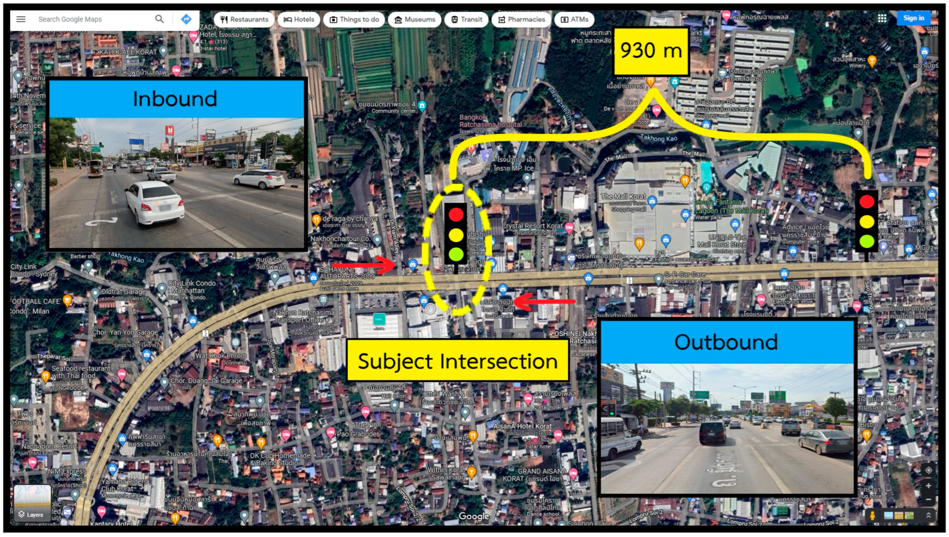
Figure 1. Area of study. The background map was captured from maps.google.com, accessed on 10 January 2023.
Sustainability 15 03466 g001
Figure 2. Example of length measurement using the Google Maps color-code data. The background map was captured from maps.google.com, accessed on 10 January 2023.
Sustainability 15 03466 g002
Figure 3. Distribution of observers and cameras in the study area.
Sustainability 15 03466 g003
Figure 4. Scenarios and models used for estimating the queue length.
Sustainability 15 03466 g004
Figure 5. Overall modeling and analysis procedures.
Sustainability 15 03466 g005
Figure 6. RMSE values for IV3 of each method and scenario.
Sustainability 15 03466 g006
Figure 7. MAPE values for IV3 of each method and scenario.
Sustainability 15 03466 g007
Figure 8. Predicted results in Scenario 3 with IV3 using the Average method.
Sustainability 15 03466 g008
Figure 9. Predicted results in Scenario 3 with IV3 using the RF method.
Sustainability 15 03466 g009
Figure 10. Predicted results in Scenario 3 with IV3 using the GBM method.
Sustainability 15 03466 g010
Figure 11. Variable importance (VI) analysis of Model 4, Scenario 3 with IV3.
Sustainability 15 03466 g011
Figure 12. Variable importance (VI) analysis of Model 5, Scenario 3 with IV3.
Sustainability 15 03466 g012
Figure 13. Variable importance (VI) analysis of Model 6, Scenario 3 with IV3.
Sustainability 15 03466 g013
Figure 14. Variable importance (VI) analysis of Model 7, Scenario 3 with IV3.
Sustainability 15 03466 g014
Table 1. Sample data obtained from Google Maps.
ItemsColorLength (m)
1st color from stop lineDark red120
2nd color from stop lineRed120
3rd color from stop lineOrange220
4th color from stop lineGreen9999
Table 2. New modified color-code variables.
Set of Independent
Variables (IV)
ColorName of Independent Variable
1st Band2nd Band3rd Band
IV1Dark redDARKRED_1DARKRED_2DARKRED_3
RedRED_1RED_2RED_3
OrangeORANGE_1ORANGE_2ORANGE_3
GreenGREEN_1GREEN_2GREEN_3
IV2Combined redC_RED_1C_RED_2C_RED_3
OrangeORANGE_1ORANGE_2ORANGE_3
GreenGREEN_1GREEN_2GREEN_3
IV3Combined redC_RED_1C_RED_2C_RED_3
OrangeORANGE_1ORANGE_2ORANGE_3
Table 3. RMSE and MAPE values of all models.
Type of VariableRandom ForestGradient BoostingAverage
RMSE
(Meters)
MAPE
(%)
RMSE
(Meters)
MAPE
(%)
RMSE
(Meters)
MAPE
(%)
Scenario 1
- IV171.833763.627472.767963.407083.907771.8533
- IV272.615364.551472.065764.046383.907771.8533
- IV372.591964.533672.674664.350183.907771.8533
Scenario 2
- IV172.176063.492172.706263.700981.828570.7399
- IV271.839563.926672.261563.305681.828570.7399
- IV371.959764.581773.252164.158781.828570.7399
Scenario 3
- IV172.049663.417472.595262.842381.613170.4689
- IV272.214463.869471.968662.988681.613170.4689
- IV371.617063.827872.354662.830481.613170.4689
Table 4. Variable importance (VI) analysis of Scenario 3 with IV3.
M4M5M6M7
VariableVI (%)VariableVI (%)VariableVI (%)VariableVI (%)
C_RED_229.616C_RED_226.472C_RED_327.398ORANGE_220.750
C_RED_121.448C_RED_125.219ORANGE_220.467ORANGE_119.297
C_RED_318.730ORANGE_217.233C_RED_214.254C_RED_116.482
ORANGE_111.948C_RED_311.453ORANGE_314.222C_RED_316.192
ORANGE_39.398ORANGE_311.244ORANGE_112.813ORANGE_314.517
ORANGE_28.857ORANGE_18.376C_RED_110.844C_RED_212.759
Disclaimer/Publisher’s Note: The statements, opinions and data contained in all publications are solely those of the individual author(s) and contributor(s) and not of MDPI and/or the editor(s). MDPI and/or the editor(s) disclaim responsibility for any injury to people or property resulting from any ideas, methods, instructions or products referred to in the content.