Energy Cost Assessment and Optimization of Post-COVID-19 Building Ventilation Strategies

Abstract

The advent of the COVID-19 pandemic puts stress on the requirements of indoor air quality. Significant improvements in the design of building ventilation systems have become necessary, as this allows for the supply of higher quantities of outdoor air in buildings. Additional capital investment is necessary for increases in the size of ventilation fans and ducts, as well as for the installation of efficient air-to-air recuperators, to recover the enthalpy of the rejected air. To address the increased operation costs, smart strategies are necessary to make rational use of the ventilation system. The required modifications are studied in the example of an 18-zone office building located in Volos, Greece. The building’s energy performance is studied by means of transient simulation. Operation of the ground-coupled heat pump, the upgraded ventilation system and the high-performance recuperators and filters’ interactions is presented in detail at various time scales. The results show the effect of increased ventilation requirements of new and renovated office and commercial buildings in the post-COVID era. The added capital equipment and operation costs must be met with a strong and sustained engineering effort. Especially in the case of nZEB buildings, the protection of public health must be attained, with reduction of the added electricity consumption penalties, in order to keep the nZEB character of the building.

1. Introduction

Nearly zero energy buildings (nZEB) are now a reality in most developed economies. The nZEB designation refers to a building that has a very high energy performance, and the very low amount of energy required per square meter should be covered to a very significant extent by renewable sources, mostly produced on-site [1]. These buildings combine a well-insulated building’s shell and structure, the exploitation of smart features of the buildings management systems and the installation of efficient heat pumps and high-performance rooftop photovoltaics. Following Article 9 of the EU Energy Performance of Buildings Directive 2010/31/EU (EPBD) [2], all new buildings constructed within the EU starting from 2021 must be nZEBs. This is implemented to a large extent, although there are wide differences across Member States in terms of nZEB implementation [3]. In parallel, a gradual electrification of buildings is carried out, which is necessary in order to contribute to the wider objective of highly energy-efficient and decarbonized buildings by 2050. Building heating is increasingly implemented by the use of high-performance heat pumps, with a wide penetration of ground-source [4] or dual-source heat pumps [5] at the core of their heating, ventilating and air-conditioning (HVAC) systems. Since nZEBs are normally producers of electricity, their high energy-efficiency frequently leads to an electricity surplus during the day, which can be profitably expended for charging the increasingly electrified cars of employees or occupants [6,7]. However, there exists an important building energy consumption source that tends to move in the opposite direction, becoming increasingly demanding. This is the building ventilation requirement, which is essential to a healthy building. Indoor air quality (IAQ), which has been considered in the past as a more-or-less subjective issue by building designers and owners, emerged to the foreground after 1990, due to the adverse effects of poor IAQ expressed by various instances of sick buildings. This requirement has been hard-coded in the newer editions of ASHRAE Standard 62 and the respective European norms after the year 2000 [8], because poor IAQ hinders the employees’ productivity in commercial and office buildings and discourages house tenants from renewing their leases. As of 1989, the requirements for space ventilation rates changed from 5 cfm per occupant to 15 or 20 cfm, depending on occupancy mode. ASHRAE Standards 62.1 and 62.2 guide the design, startup, operation and maintenance of commercial, institutional and residential ventilation systems [9]. As “continuous maintenance” standards, they are modified and updated every three years to incorporate all addenda approved in-between [10]. Acceptable indoor air quality can be achieved via the control of contaminant sources, adequate ventilation rates, management of humidity and supply and return air filtration. Apart from microbial contamination, particles or chemicals originate from occupants’ presence and activity, as well as from furniture and wall and floor coatings. They may infiltrate the building along with the air, or be transported along with the outdoor air introduced to the ventilation system. Obviously, controlling contaminants as close to the source as possible, which is the more cost-effective strategy, is not always possible. In most cases, dilution with outdoor air is the only possible approach. ASHRAE Standard 62.1 describes two procedures to calculate the necessary ventilation rates to dilute these contaminants. The most frequently applied is the Indoor Air Quality procedure, which determines minimum design ventilation rates (L/s outdoor air $q_{\mathrm{tot}}$) based on the following formula:

$$q_{\mathrm{tot}}=n\cdot q_p+A_R\cdot q_B$$

(1)

where $q_{\mathrm{tot}}$ is the total ventilation rate for the breathing zone, $n$ is the normal number of occupants, $q_p$ is the ventilation rate per person (L/s), $A_R$ is the floor area (m²) and $q_B$ (L/m²s) is the ventilation rate needed to dilute emissions from building surfaces. The above ventilation rates refer to well-mixed conditions, with uniform contaminant concentration levels. They also assume 100% ventilation effectiveness, which means that all outdoor air delivered by the ventilation system reaches the occupied zone. On the other hand, ventilation systems for spaces with intermittent or variable occupancy are separately addressed. Adjustment of their outdoor air quantity is allowed to provide the necessary dilution for acceptable levels of contaminant concentration [9]. The advent of the COVID-19 pandemic significantly challenged buildings’ ventilation systems [11]. This is due to the convergence of all research works to the conclusion that airborne transmission is the major propagation mode of COVID-19 in enclosed spaces [12]. High transmission rates have been reported when susceptible individuals are close (1–2 m) to an infected person. Droplet spray and inhalation exposure are intense in such small distances. However, transmission is also possible with several meters of distance inside a room [13]. It takes only 2 s for droplets to evaporate and leave drier, smaller particles (droplet nuclei), that are more easily swept by air motion, since their drag forces are comparable to gravity [14]. This allows the virus particles inside the nuclei to survive for one hour or more suspended in the air, since the size of coronavirus particle ranges from 80 to 160 nm [15]. Elsaid et al. [16] commented on the design of existing air-conditioners, as regards their impact on the spread of the coronavirus. They reviewed efforts to develop highly efficient air filters and ionizers for protection against epidemic infection. Hamdani et al. [17] conducted experiments with a full-scale negative pressure isolation room for COVID-19 patients at Syiah Kuala University to investigate the performance improvements in terms of temperature, pressure, humidity and energy consumption with a computer HVAC control system. Wide research experience from the pandemic made clear that adequate ventilation is essential to reduce the spread of respiratory viruses [18]. Alonso et al. [19] conducted onsite measurements of environmental variables in primary schools with mechanical ventilation systems in Spain, before and during the pandemic. They found a decrease of 300 ppm in CO₂ weekly average values during the pandemic with hybrid ventilation and a decrease of 400 ppm with natural ventilation during all teaching hours. Fageha et al. [20] proposed an optimized natural ventilation strategy in educational buildings to minimize the probability of viral infection and avoid draught discomfort by means of a building energy simulation tool, coupled with the Wells–Riley equation for probability of infection and Fanger’s draught equation to estimate the draught risk. Haohan et al. [21] investigated the relationship between infection risk and ventilation rate. They also examined optimal ventilation control for dilution ventilation and ventilation cooling. Wang et al. [22] aimed their study towards balancing a low-infection-risk with energy-efficient ventilation control. They proposed a smart, low-cost ventilation control strategy based on occupant density detection. According to the US Environmental Protection Agency (EPA), increased ventilation with outdoor air is a key engineering measure to reduce indoor air-pollutants or contaminants, including airborne viruses [23]. Mohammadi et al. [24] evaluated the transmission of outdoor pollutants into the indoor environment using 3D computational fluid dynamics with a pollution-dispersion model. Naturally ventilated buildings next to an urban canyon were modelled and validated against wind tunnel results from the Concentration Data of Street Canyons database. Pampati et al. [25] reviewed school-based strategies to improve ventilation to reduce incidences of COVID-19 in a nationally representative sample of U.S. K–12 public schools. They concluded that improved outdoor air ventilation is the key strategy recommended to reduce COVID-19 spread in school settings. Marotta et al. [26] reviewed strategies developed by several Sustainability Rating Systems to respond to any infectious disease and ensure that building occupants protect and maintain their health. The best practices point to an overall sustainability increase with resilience. The decomposition of the concept of sustainability in its three components (environmental, social and economic) shows that preventive strategies are likely to be systematically adopted as state-of-the-art. A well-documented study conducted by experts from the Federation of European Heating, Ventilation and Air Conditioning Associations (REHVA), points to the preventive direction. Following the collection of available evidence, a health-based ventilation design methodology was proposed [27]. In Europe and elsewhere, the current ventilation design, based on EN 16798-1:2019 [28] and ISO 17772-1:2017, is based on perceived air quality (odors) and has neglected respiratory disease transmission. REHVA proposed an infection-risk-based ventilation design method to provide new target ventilation rates in non-residential buildings, excluding healthcare and industrial buildings. Health-based ventilation rates are generally higher than those based on comfort conditions and are mandatory during epidemic periods. Moreover, to save energy in variable-occupancy spaces, Standard 62.1 allowed a calculated minimum space ventilation rate based on average space occupancy whenever peak occupancies were of short duration. Such provisions could no longer be applied under the new situation with the existence of highly contagious viral infections, such as COVID-19. This would further increase the required outdoor air quantities, as detailed in this study. Furthermore, the present study investigates the additional equipment and operational measures required to fulfill the increased outdoor ventilation rates for the case of an 18-zone nZEB office building, equipped with a rooftop PV installation, and space heating and cooling performed by a high-efficiency ground-source heat pump system. Moreover, the effect of the additional electricity consumption penalty induced by the updated ventilation requirements on an office building’s nZEB character is examined for the first time, according to the authors’ knowledge. Finally, specific strategies to minimize the electricity consumption penalty are discussed. This paper is organized in four sections. Section 2 presents the overview of the building’s HVAC system and input data for the transient simulation, with special emphasis to the computation of the ventilation system performance, according to the different scenarios. Section 3 presents and discusses the simulation results. The conclusions and future work are presented in Section 4.

2. Materials and Methods

The office building’s transient performance is investigated in the TRNSYS 16 simulation environment. Due to its modular structure, this software is routinely applied to understand and optimize similar cases of complex thermal systems. The transient operation of critical system components, such as the air-source heat pumps [29] or ground-coupled heat pumps [30], can be profitably studied in this environment. This allows for the study of component sizing for different climate types and building operation schedules [31]. Input data and component interactions are inserted in a graphical user interface. The simulation engine solves the resulting system of linear equations. This software has demonstrated a good fit to test results during the simulation of ground-source heat pump operations [32]. The comparative performance of TRNSYS against other standard building energy simulation software is presented in [33]. It is a certified building energy analysis software in the framework of ANSI/ASHRAE Standard 140-2001 [34]. In this section, the basic structure of the system’s model employed in the transient simulation is described, along with the building’s details and schedules, with special emphasis to the structure and modeling of the HVAC and ventilation system. As regards the size of the various components, the following philosophy was adopted: The building has been designed as a nZEB, with a HVAC system based on an efficient ground-coupled heat pump. The nZEB character of the building must be retained, which means that the annual energy balance should be kept positive (the building should be a net exporter to the grid). The flat roof of the building is used for the rooftop PV installation, along with the sixteen Air-handling Units (AHU) for the ventilation of all zones, except for the parking zone. This last zone, located in the basement, is equipped with a separate ventilation system based on wall ventilators for air supply and exhaust. The sizing of the rooftop PV installation was based on the available space (Figure 1).

2.1. Building Simulation Details

The 4-story office building (typical floor plan in Figure 1) has a ground trace of 1340 m² (84 × 16 m). A maximum number of 150 occupants is assumed during weekdays. An 80-car capacity parking zone lies in the basement, with 20 places equipped with 7 kW, 3-phase, 32 A/400 V electric car chargers.

The main building shell insulation data are presented in

Table A1. Building insulation data (U-values).

Shell Type	Layers	U (W/m2K)
Roof insulation	Reinforced concrete slab, extruded polystyrene, lightweight concrete, ceramic tiles	0.272
Concrete column	Reinforced concrete, extruded polystyrene	0.324
Outside wall	Ceramic brick, extruded polystyrene, ceramic brick	0.319
Floor insulation	Reinforced concrete slab, extruded polystyrene	0.443

, Appendix A. These include energy-efficient windows and automatic shading devices for the summer. This results in the summer cooling loads kept at similar levels as the winter heating loads. The total floor area is 6700 m², out of which the conditioned zones area is 5750 m². The ceiling height is 3 m for all levels above ground. The basement has a ceiling height of 4 m, hosting electromechanical installations and parking places. The level roof has a total of 315 PV panels (1134 × 1722 mm, 415 Wp nominal output) facing SSW in a portrait orientation (Figure 1) and at a 20 degree tilt angle. They produce a nominal 130.7 kW peak power. Meteorological data are introduced by means of a typical meteorological year (TMY) for the city of Volos, Greece. This comprises 8760 hourly input values of ambient Dry Bulb temperature, relative humidity, wind direction and speed and total/direct solar horizontal radiation.

2.2. HVAC System Details and Heat Pump Submodel

The technical data of the water–to-water heat pump are listed in

Table A2. Water–water heat pump efficiency data for heating and cooling modes.

	Heating Mode: Ground Loop Water Temperature [°C]
	18.0	15.0		13.0	10.0	8.5		7.0	4.5	2.0		0.0
kW thermal	271.4	255.4		241.9	228.8	216.0		209.7	193.2	183.0		173.0
KW	46.8	45.6		44.8	44	43.2		42.8	42	41.6		41.2
COP	5.8	5.6		5.4	5.2	5		4.9	4.6	4.4		4.2
Cooling Mode: Ground Loop Water Temperature [°C]
	20		25		30		35		40		45
kW thermal	201.6		198.9		196.1		194.2		185.6		177.8
kW	48		51		53		55.5		58		63.5
COP	4.2		3.9		3.7		3.5		3.2		2.8

—Appendix A. The heat pump receives or discharges heat to a ground network consisting of eighty ∅200 mm × 80 m depth boreholes. It is capable of supplying up to 210 kW of heating at 7 °C outdoor DB temperature, and 195 kW of cooling at 35 °C. It produces hot or cold water that feeds fan coil units to cover the heating and cooling loads for all office spaces in the building. Six rooftop air-handling units (Figure 1), and another four on the ground floor, are employed only to cover the ventilation needs of all zones except the basement. This keeps the air transportation needs to a minimum, minimizes the size of air ducts and allows greater flexibility in regulating air flow for each zone. All air-handling units are set to 100% outdoor air (Figure 2) and are equipped with high-performance recuperators to reclaim up to 70% of the exhausted air’s enthalpy. They are also typically equipped with pre-filters and bag filters. Efficient LED lighting and high-efficiency (A+) electrical equipment is installed. The heat pump model follows Type 668 [35]. The year-round heat transfer operation of the vertical U-tube ground loop is modeled based on Type 557a [35].

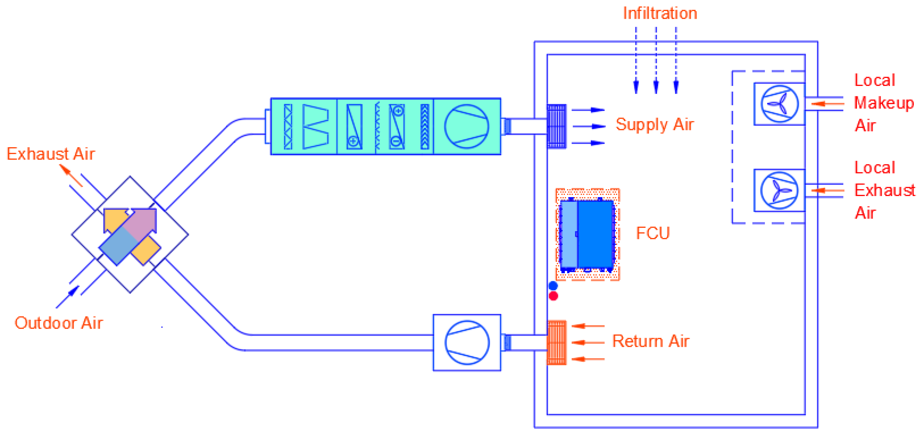
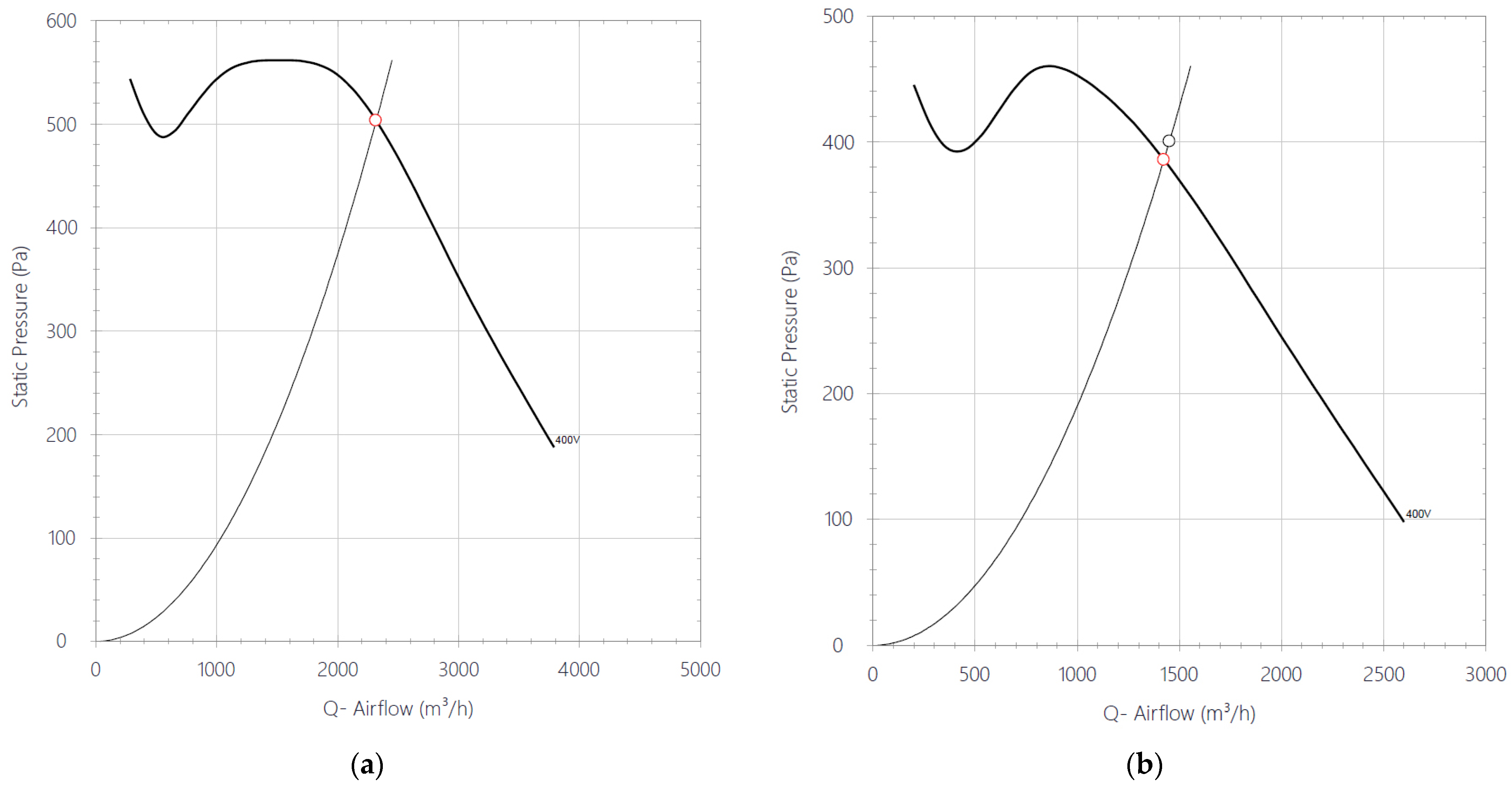
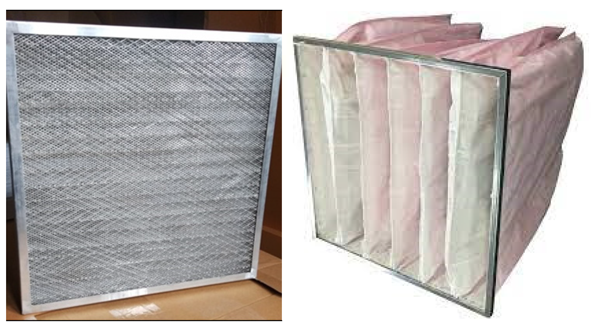
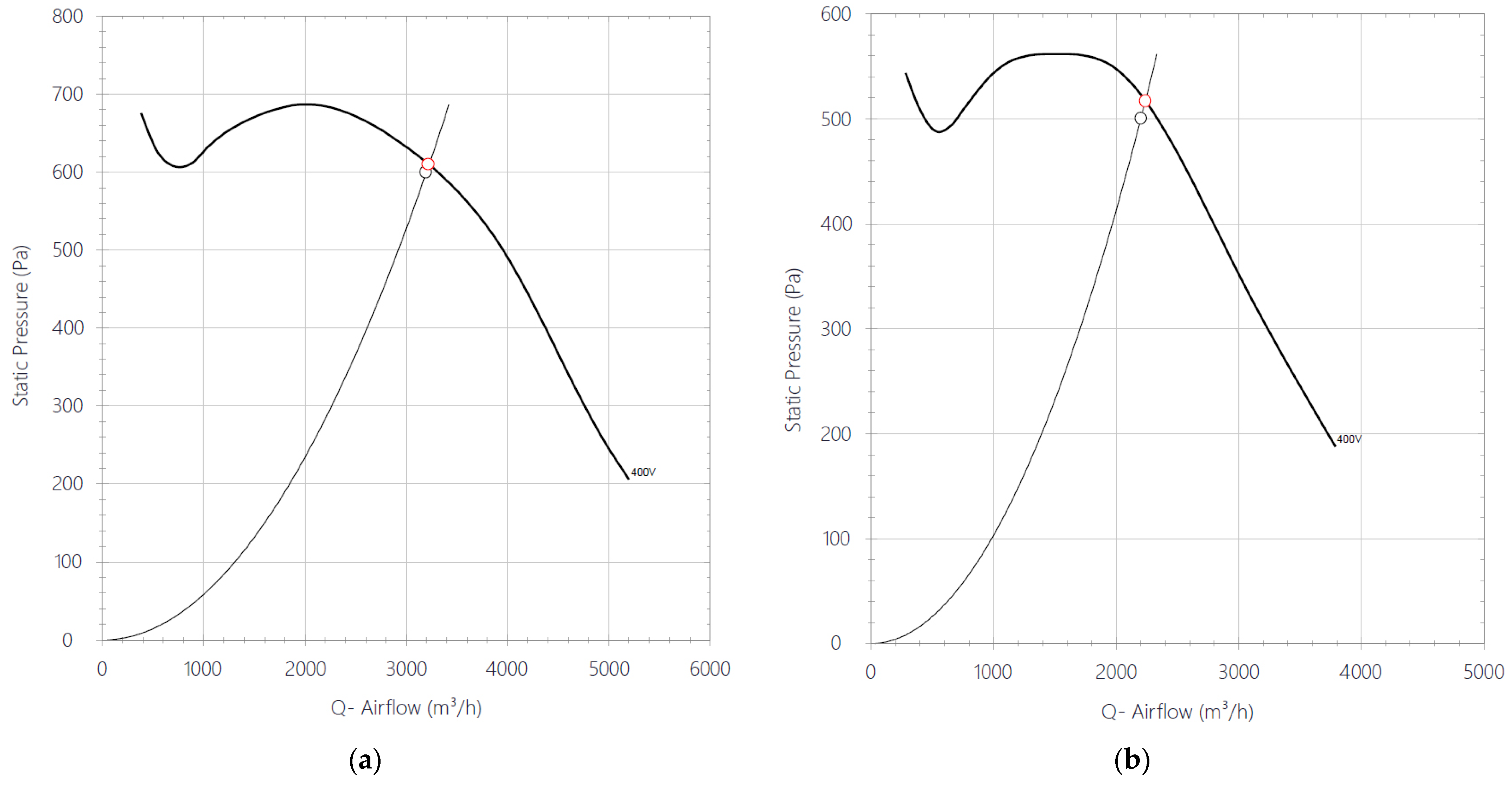
2.3. Air-Handling Units, Details of Centrifugal Fan Characteristics, Filters, Recuperators

As mentioned above, the ventilation air for each zone is furnished by an air-handling unit of the general type shown in Figure 2. These units are supplying 100% outdoor air (no recirculation is permitted) and are equipped with recuperators for the pre-heating or pre-cooling of the outdoor air introduced to the system. Now, according to the detailed calculations, the system must be capable of supplying a maximum of 19,000 m³/h outdoor air to the specific building under study, in order to cover the requirements of EN 16798-1:2019 for Category II, which is the normal level used for new buildings and renovations (see

Table 1. Description of the applicability of the indoor environment categories used in EN 15251 and EN 16798-1:2019 [28].

Category	Explanation	$\mathbf{Ventilation} \mathbf{Rate} {\mathit{q}}_{\mathit{B}} (\mathbf{L}/{\mathbf{m}}^{\mathbf{2}}\mathbf{s}) (\mathbf{Equation} (1\left)\right)$
I	High level of expectation: recommended for spaces occupied by very sensitive, fragile persons with special requirements: handicapped, sick, very young children, elderly persons	1
II	Normal level of expectation: should be used for new buildings and renovations	0.7
III	An acceptable, moderate level of expectation: may be used for existing buildings	0.4

).

This quantity is supplied by six rooftop AHU of 2200 m³/h capacity each and another four AHU of 1450 m³/h capacity placed at ground level. The 2200 m³/h nominal flow rate of each of the larger AHU is supplied by a fan with characteristics shown in Figure 3a, powered by a direct-drive, 3-phase, 1.1 kW motor. The associated exhaust fan is powered by a 3-phase, 0.55 kW motor. The 1450 m³/h nominal flow rate of each of the smaller-sized AHU is attained by a supply fan with characteristics in Figure 3b, powered by a direct-drive, 3-phase, 0.55 kW motor and an exhaust fan powered by a single-phase, 0.40 kW motor [36]. As indicated by the respective characteristics of the centrifugal fans in Figure 3, the static pressure head at their design points approaches 500 and 400 Pa, respectively.

Typical pre-filter (Figure 4a) and bag filters (Figure 4b) are installed in the supply side of each AHU. HEPA filters are not installed, due to the high backpressure levels involved.

2.4. Photovoltaic Installation Modeling

The detailed PV operation model is based on [37] to reconstruct the module’s I-V curve by fitting data from the manufacturer’s datasheet. The cell is viewed as an equivalent, single-diode circuit. The following values are fitted to the main model parameters: I_L (the light current, I_L,f = 10.85 A), I₀ (reverse diode current, I₀ = 0.299 nA), R_S (module series resistance, R_S = 0.0605 Ω), R_SH (shunt resistance, R_SH = 5000 Ω), and α (modified ideality factor, α = 2.664). The panel’s I–V curve is reconstructed according to the following equation:

$$I=I_L-I_0\left(e^{\frac{V+I{R}_S}{\alpha }}-1\right)-\frac{V+I{R}_S}{R_{SH}}$$

(2)

The modified ideality factor α depends on the cell temperature T_C, the number of cells in series N_S, the usual ideality factor ${\eta }_I$, the Boltzmann constant k and electron charge q. The above-stated model parameter values were extracted by solving the de Soto model equations to fit the data provided in the manufacturers data sheet of

Table 2. Technical data of the 415 Wp monocrystalline silicon, 120 half-cells PV panels NU JC415 [38], as used in TRNSYS type194.

PV Module Parameter	Value	Comments
ISC at STC	13.87 A	Short circuit current
VOC at STC	38.08 V	Open circuit voltage
IMPP at STC	13.18 A	Current at max power point
VMPP at STC	31.49 V	Voltage at max power point
Temp. coefficient of ISC (STC)	0.054%/K	αISC
Temp. coefficient of VOC (STC)	−0.262%/K	βVOC
Number of cells wired in series	2 strings × 60	modules
Module temperature at NOCT	315.5 K
Ambient temperature at NOCT	293 K
Module area	1.95 m2
Module efficiency	21.25%

[38]. In this way, the full I-V curve for the panel is produced for the modeling.

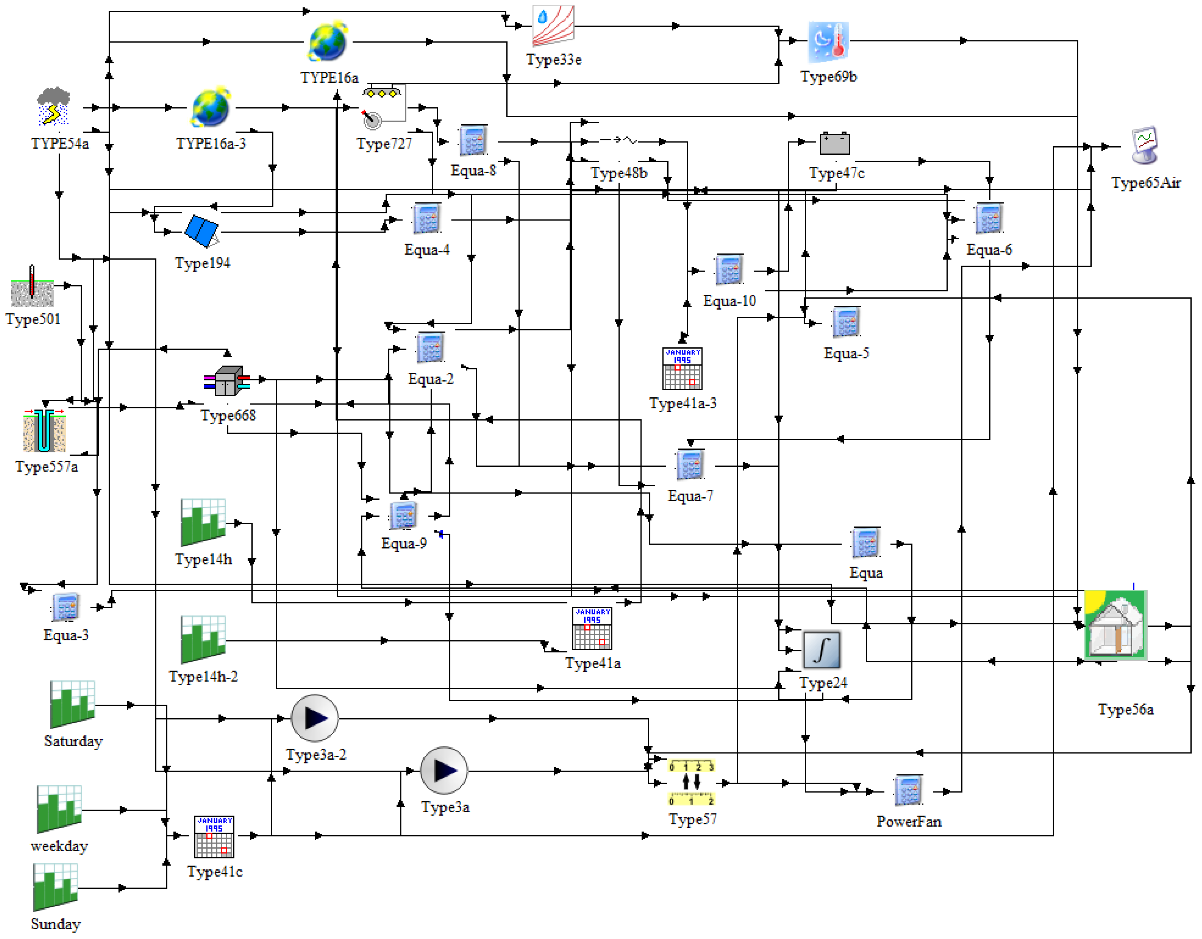
2.5. TRNSYS 16 Types and Simulation Details

The basic component of the system model is the 18-zone model of the office building (Type 56). Other components include Type 54 (weather generator), Type 16 (solar radiation processor), Type 69 (effective sky temperature), Type 501 (ground temperature calculation) and Type 33 (psychrometrics). Electrical components include Type 194 (PV panels), Type 48a (inverter), Type 668 (heat pump), Type 557a (ground heat exchangers) and Type 3a (ventilation fans). All subroutines are parts of the TRNSYS 16 and TESS libraries [35].

All TRNSYS types, and their interconnection in the TRNSYS simulation studio interface, are presented in Figure 5.

2.6. Increased Outdoor Air Requirements during COVID-19 Episodes

As explained in the introduction section, increased outdoor air capacities are expected to be available in new buildings of the post-COVID-19 era. This increased capacity would be exploited, in order to allow physical presence in offices during specific episodes of COVID-19. Focused research works point to increased capacity, supported by continuous recordings of indoor air CO₂ concentration with varying occupancy in specific space categories. Increased levels of outdoor air are required to keep a rational target CO₂ concentration of 800 ppm [39]. Although the related legislation is not yet agreed, due to the significant increase in investment and, especially, operating costs for the oversized fans, a good estimate of the added burden to the ventilation system can be made if we take, as a starting point, the increased outdoor air requirements of Category I buildings with high levels of expectation for indoor air quality (Table 1), which are recommended for spaces occupied by very sensitive and fragile persons with special requirements, such as handicapped, sick, very young children and elderly persons, according to the European Standard EN 16798-1:2019 [28]. By adhering to these assumptions, the detailed calculations show that the system must be capable to supply a maximum of 27,000 m³/h outdoor air to the building.

This increased quantity can be supplied by the same number of ten Air-handling Units, which now need to be oversized as follows: six rooftop AHU of 3100 m³/h capacity each and four AHU of 2100 m³/h capacity each placed at ground level. The 3100 m³/h nominal flowrate of each of the larger AHU would require a supply fan, with characteristics as in Figure 5a, powered by a direct-drive, 3-phase, 2.2 kW motor [36] and an associated exhaust fan, powered by a 3-phase, 1.1 kW motor. The 2100 m³/h nominal flowrate of each smaller-sized AHU would require a supply fan with characteristics as in Figure 5b, powered by a direct-drive, 3-phase, 1.1 kW motor and an exhaust fan, powered by a 3-phase, 0.55 kW motor [36]. As indicated on the respective characteristics of the centrifugal fans in Figure 6, the static pressure head at their design points is close to 600 and 500 Pa, respectively.

As expected, the oversized equipment would be operated in demand-driven ventilation mode, which means that, during the normal operation (outside of COVID-19 episodes), the ventilator motors will be regulated at a reduced speed by their inverters. In the next section, an assessment of the increase in operating costs involved is carried out by means of the comparative building energy simulation runs of the two alternative ventilation systems.

It must be noted in this context that the increased ventilation rates, apart from the increased ventilators’ electricity consumption, induce additional heating or cooling by the heat pump in order to bring the outdoor air to the required indoor temperature (known as ventilation load). This effect is included in the building energy simulation and reported in the results. The effectiveness of the recuperators that are present in all Air-handling Units is taken into account for the ventilation load computations.

3. Results and Discussion

The original results of the transient simulation include a 0.1 h time resolution of several outdoor and indoor environment variables. In addition, the main building electricity consumption variables are presented to describe the electrical system’s behavior, as well as the following variables, describing the electric power interaction of the building with the external grid:

(i) The electric power imported from the grid when the photovoltaic production cannot cover the building’s demand; (ii) The power surplus, which is the difference between electric power that is produced by the rooftop PV installation and consumed by the HVAC system, lighting and electric appliances. This is managed by the building’s management system and can be exploited by charging the employees’ EVs, or can be exported to the electricity grid; (iii) The power exported to the grid, which is calculated after subtraction from the power surplus of the electric power that is possibly consumed by employees’ electric cars’ batteries charging.

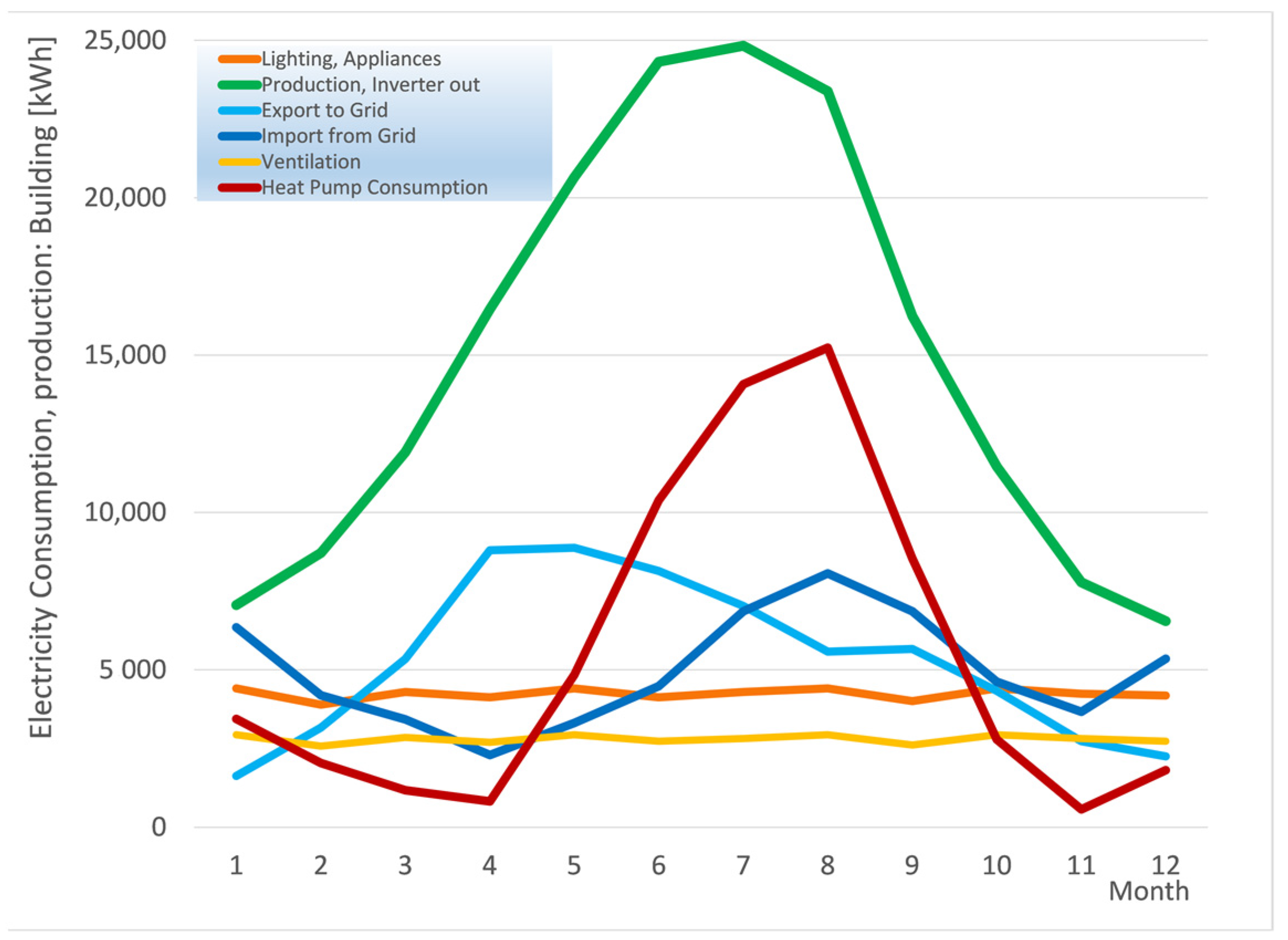
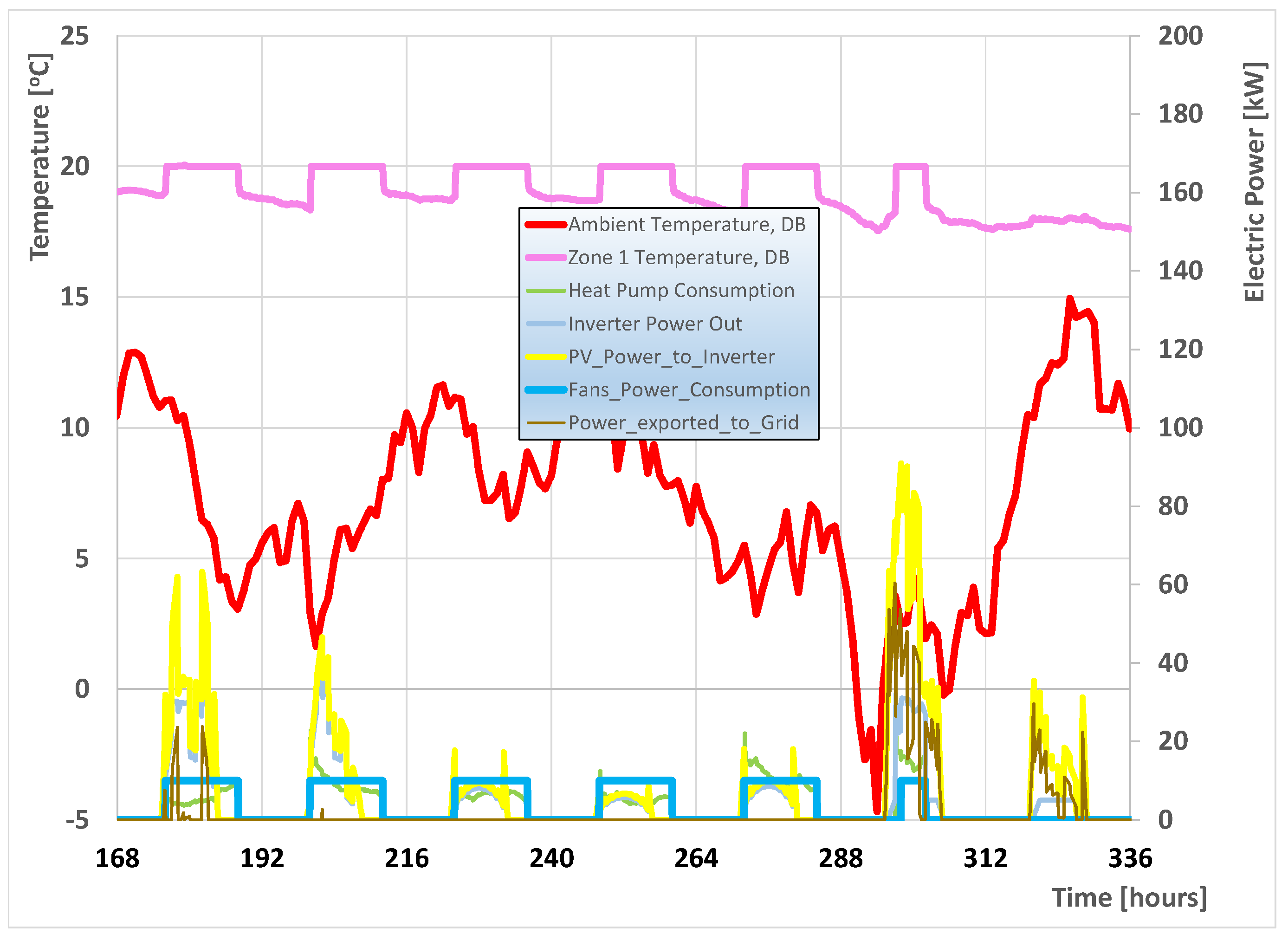
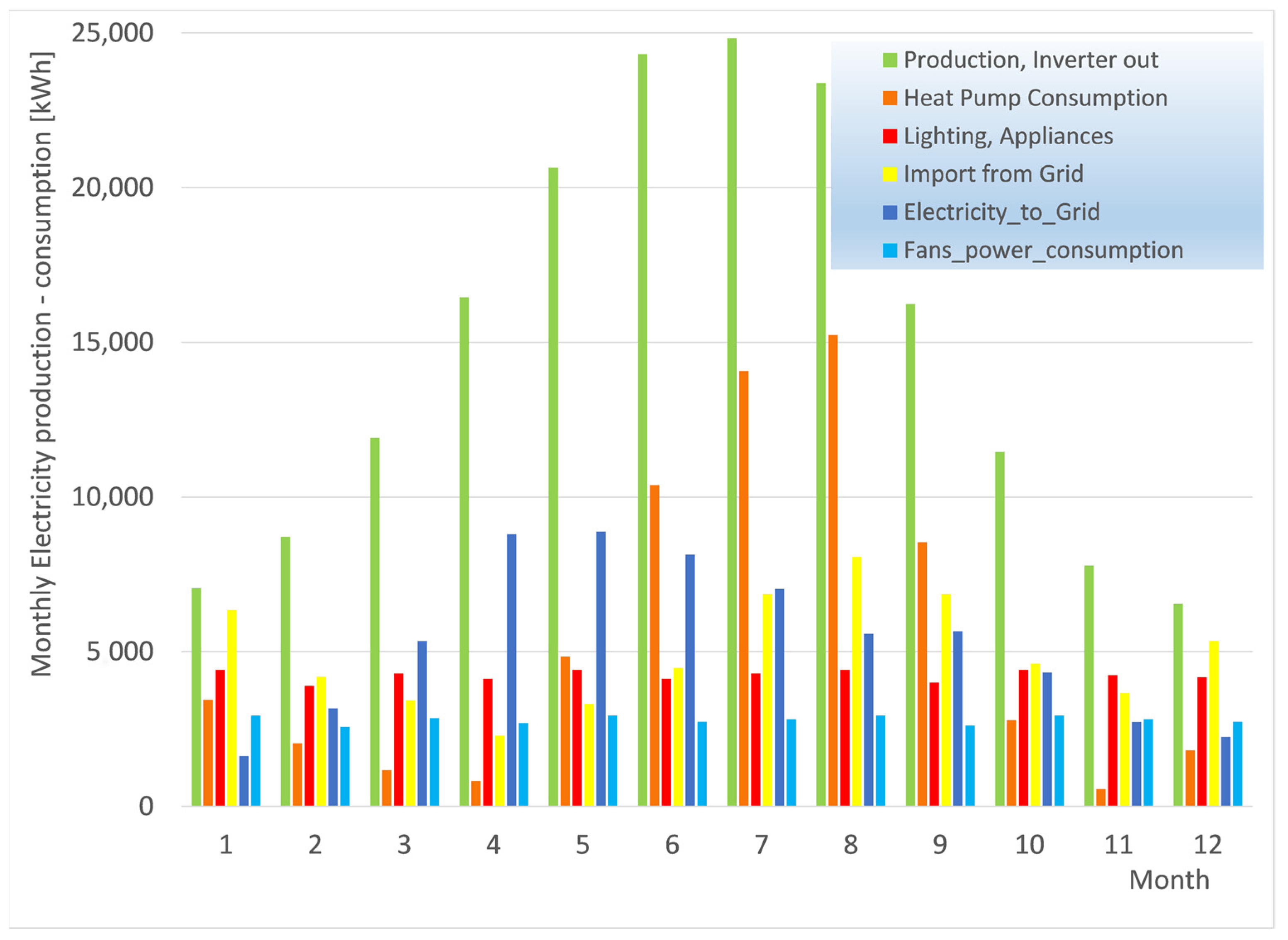
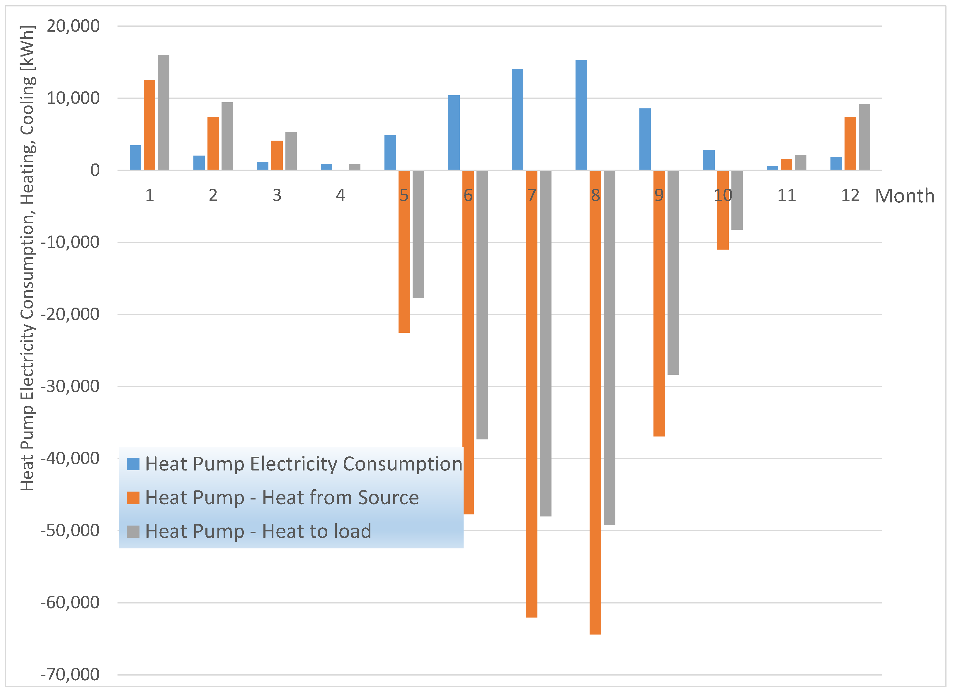
3.1. Monthly System’s Performance and Annual Summary—Baseline Building

The overall system’s performance can be assessed by means of monthly energy data, as presented in Figure 7. The highest PV production is observed in June and July, approaching 25,000 kWh/month, and the lowest is observed in December at 6500 kWh.

The heat pump consumption varies during the year, becoming negligible during the neutral months. The building’s electricity consumption for the lighting and electrical appliances averages to less than 4500 kWh/month. The building’s annual electricity consumption is computed to the amount of 150,000 kWh, or about 26 kWh/m²y. This corresponds to 75.5 kWh/m²y primary energy consumption, where the limit set by the European legislation for an nZEB building is 80–90 kWh/m²y total primary energy consumption [40]. The total annual electricity produced by the PV installation is predicted at 179,000 kWh. The building imports from the grid a total of 59,500 kWh and exports annually 63,600 kWh. Thus, the annual building’s electricity self-production is at the same levels with its annual consumption, which confirms the building’s nZEB character. On a monthly basis, we observe in Figure 6 that the building is a net electricity consumer during the seven months from August to February. During the remaining five months of the year, it becomes a net exporter to the grid. Before exporting the surplus quantity to the grid during the surplus period, there exists the additional possibility of charging an average of 20 employees’ electric cars during the week days, which would consume 200 kWh per working day (4400 kWh/month). Selling this quantity to the employees which are owners of electric cars can be beneficial to the building, because the charging period coincides with the hours of sunshine. Obviously, it is important to study the specific hours of the day where the building is importing or exporting to the grid. This will be carried out during the study of the hourly building energy performance in the sequel. An examination of the variation of energy production and consumption in Figure 6 justifies the selection of the 20° panels’ tilt angle mentioned above. By this specific choice, the rooftop PV installation is optimized for summer operation, where the need is higher, due to the increased HVAC cooling loads. These data are examined in more detail in Figure 8.

The seasonal heating and cooling energy production, along with the electricity consumption, are presented in Figure 8. The heat gain from the ground during winter is added to the compressor work, and the total is transferred to the load in heating mode. During cooling mode operation, the heat absorbed from the load is added to the compressor’s work and rejected to the ground. The monthly average coefficient of performance (COP) varies between 4.4–5.6 in heating and 3.2–4.0 in cooling. The summer cooling loads significantly exceed the winter heating loads. This is due to the local climate, which has mild winters and hot summers. It should be mentioned that the actual operation of ground-source heat pumps may deviate significantly from the theoretical design predictions [41], due to the uncertainty regarding the variation of ground thermophysical properties in the neighborhood of the boreholes [42]. This is related to the incomplete knowledge of soil- and ground-humidity variation with depth [43]. The annual heat pump’s electricity consumption reaches 65,700 kWh (12 kWh/m²y). These low consumption levels become attainable by the good building’s shell insulation and the high-efficiency levels of the ground-source heat pump. Figure 9 shows the comparative variation of electricity exported and imported from the grid, which allows a better overview and comparison of the electricity production and consumption for various purposes in the course of the year. A comparison between the monthly electricity consumption of the heat pump with the consumption of the HVAC system fans in Figure 9 reveals that, during the winter and neutral months, they consume more electricity than the heat pump itself. That is, the transportation of the ventilation air from the outside to the building’s interior costs more than its heating.

The reverse is observed during the hot summer months, where the heat pump electricity consumption significantly exceeds that of the ventilation system fans. Overall, the ventilation system fans consume 33,600 kWh (6 kWh/m²y), which is about half of the heat pump consumption. On the other hand, the electricity consumed for the building’s lighting and the office equipment are kept at very low levels throughout the year, due to the optimal exploitation of the daylight and the high-efficiency of office equipment. Overall, the monthly electricity consumption for lighting and electrical appliances is about 50% higher than the respective power allocated to the ventilation. Further, it would be useful to know the specific hours of the day that electricity would be available (and much needed) for exportation, as discussed in detail in the next figures.

As a starting point, the system’s operation during the second week of January is presented in Figure 10, beginning on Monday. The thermostat is set to 20 °C indoor temperature in all office spaces during working hours. A significant variation of available sunshine and ambient temperatures, which affect the heating loads, produces the observed patterns, where the availability of electricity for export to the grid (or EV charging) is limited to short duration periods during Monday, and to large periods during Saturday and Sunday.

The situation changes dramatically during the neutral months of April and May, where the heat pump consumption is negligible. Moreover, there is plenty of sunshine, which keeps PV production at steadily high levels, making the building a net electricity exporter to the grid. This situation is presented in the example of Figure 11 (late April–beginning of May). Significant amounts of electricity surplus become available for export to the grid or EV charging, up to a maximum power level exceeding 12 kW at noon hours during most weekdays, and reaching 15 kW during the weekend. The total ventilation fans’ consumption stays at their nominal level, which is a total of 7 kW during the working hours. However, the advent of summer is associated with higher temperature levels, with sporadic heat waves occurring during July and August. As an example of this operation mode, Figure 12 allows an assessment of the building’s energy performance during the first days of July. The indoor temperature set point for cooling mode is set to 26 °C. The heat pump is observed to operate in cooling mode at high power levels to address the high cooling loads of the prolonged heat-wave of Monday—Tuesday, and—to a lesser extent—during the next days.

Starting from 4042 h on Monday, a steep ramp is observed in ambient temperatures. Initially, during the morning, the building’s heat capacity delays heating of the interior. The heat pump consumption is kept at low levels and, due to the maximized PV production, the building continues to keep an electricity surplus for export or EV charging. However, during the afternoon, the electricity loads are high and the building needs to import electricity. This general pattern is observed during the next days of the week. That is, the building has a surplus during the morning and needs to import certain amounts of energy during the afternoon. The ground-source heat pump demonstrates a high-efficiency in cooling operation, mainly due to the significant heat capacity of the ground.

The above observations allow for assessment of the seasonality and daily variation of the mode of interaction of the nZEB building with the grid. That is, we observe a shift from import to export mode during each day and also a seasonality of the building’s behavior, with higher export levels during the neutral months and reverse behavior during the winter and summer months. To give an annual overview and allow the assessment of the observed peaks in import and export power, Figure 13 shows the fluctuation of power from the grid and the respective power transferred to the grid on an hourly basis for one full year. Some electricity export peaks are reaching 100 kW. As already seen in the transient simulation diagrams, these instances usually do not exceed the duration of a few hours each day. These electricity exports to the grid are more frequent from May to September, where PV production is at its highest. Export to the network occurs also during the weekends throughout the year, due to a surplus of electricity because of decreased building loads. The annual total of 63,300 kWh is exported (Figure 7). At the opposite side, a total amount of 59,500 kWh is imported from the grid, being more evenly distributed during the year, peaking to 60 kW, with some rare peaks observed at 80 kW.

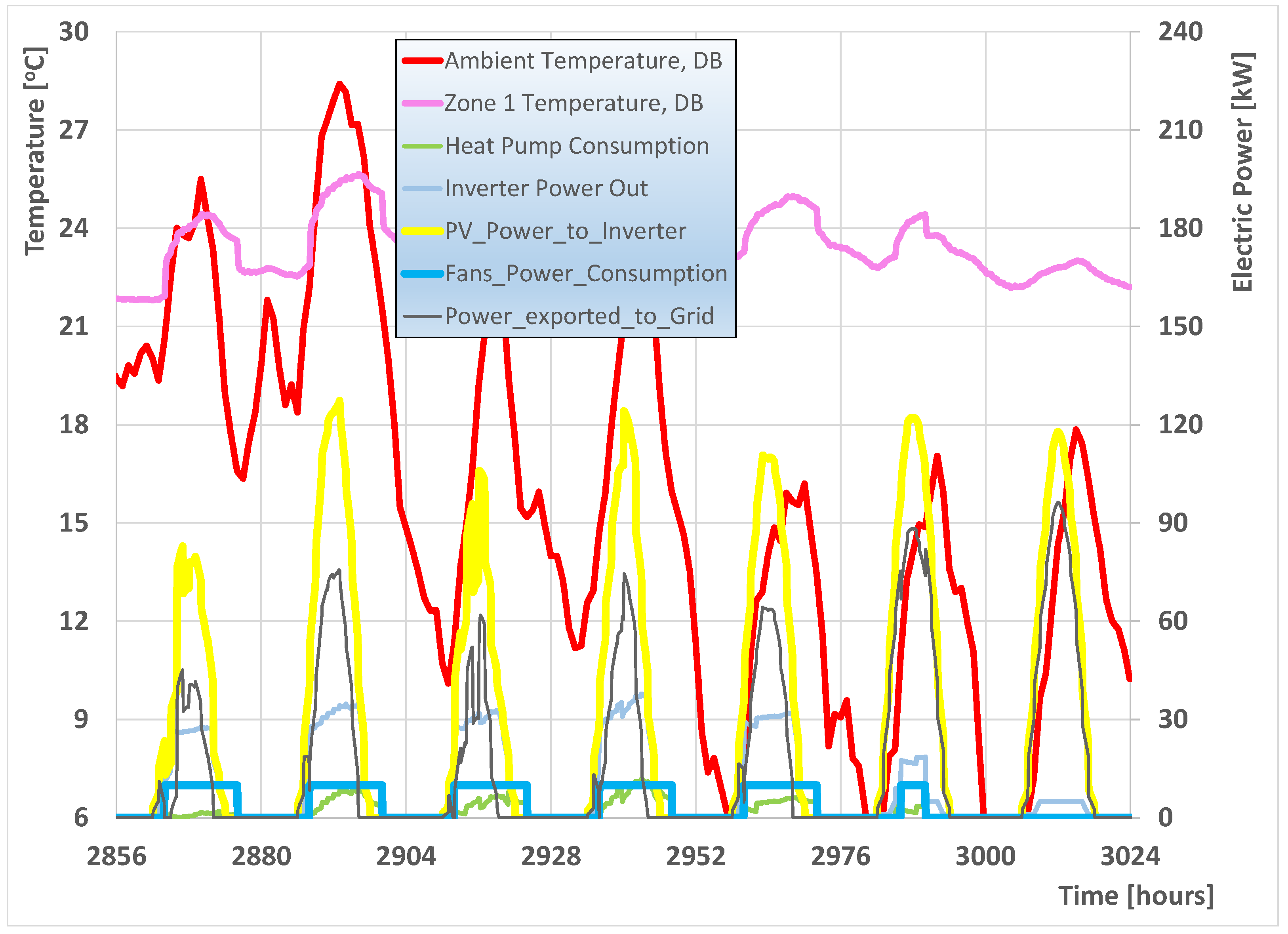
3.2. Monthly System’s Performance—Building with Increased Ventilation

The above results give a good understanding of the performance of an nZEB office building with Category II. Now, the adoption of an increased capacity for indoor air quality of Category I, which exist as extreme cases in the current European Standard and the associated ASHRAE 62, significantly affects the building’s electricity consumption, as will be demonstrated in the new simulation results. To this end, the building energy system is modeled with ten increased capacity Air-handling Units which, according to the detailed calculations, should supply a maximum of 27,000 m³/h outdoor air to the building.

The summary results for this alternative scenario is presented in Figure 14, where the comparison with the reference case of Figure 9 reveals the following important excursions of the building energy performance: (i) The ventilation fans’ annual electricity consumption has now increased to a total of 70,000 kWh. The monthly consumption of the ventilation fans is seen now to significantly exceed the remaining electricity consumption for lighting and appliances for the building; (ii) As a result of the increased ventilation fans’ consumption, and an associated smaller increase in heat pump consumption to address the increased ventilation heating and cooling loads, the monthly electricity imports from the grid are significantly increased, and the respective electricity exports have decreased. A total annual amount of 87,800 kWh is imported, and a respective 52,300 kWh is exported to the network. The building becomes a net importer of electricity with 35,500 kWh/y, or 6.18 kWh/m²y. This corresponds to 17.9 kWh/m²y net primary energy consumption of the building (current primary energy conversion coefficient for the Greek electricity generation system is 2.9). Thus, the nZEB character of the building, which requires less than 20 kWh/m²y net primary energy consumption [40], is challenged to a certain degree.

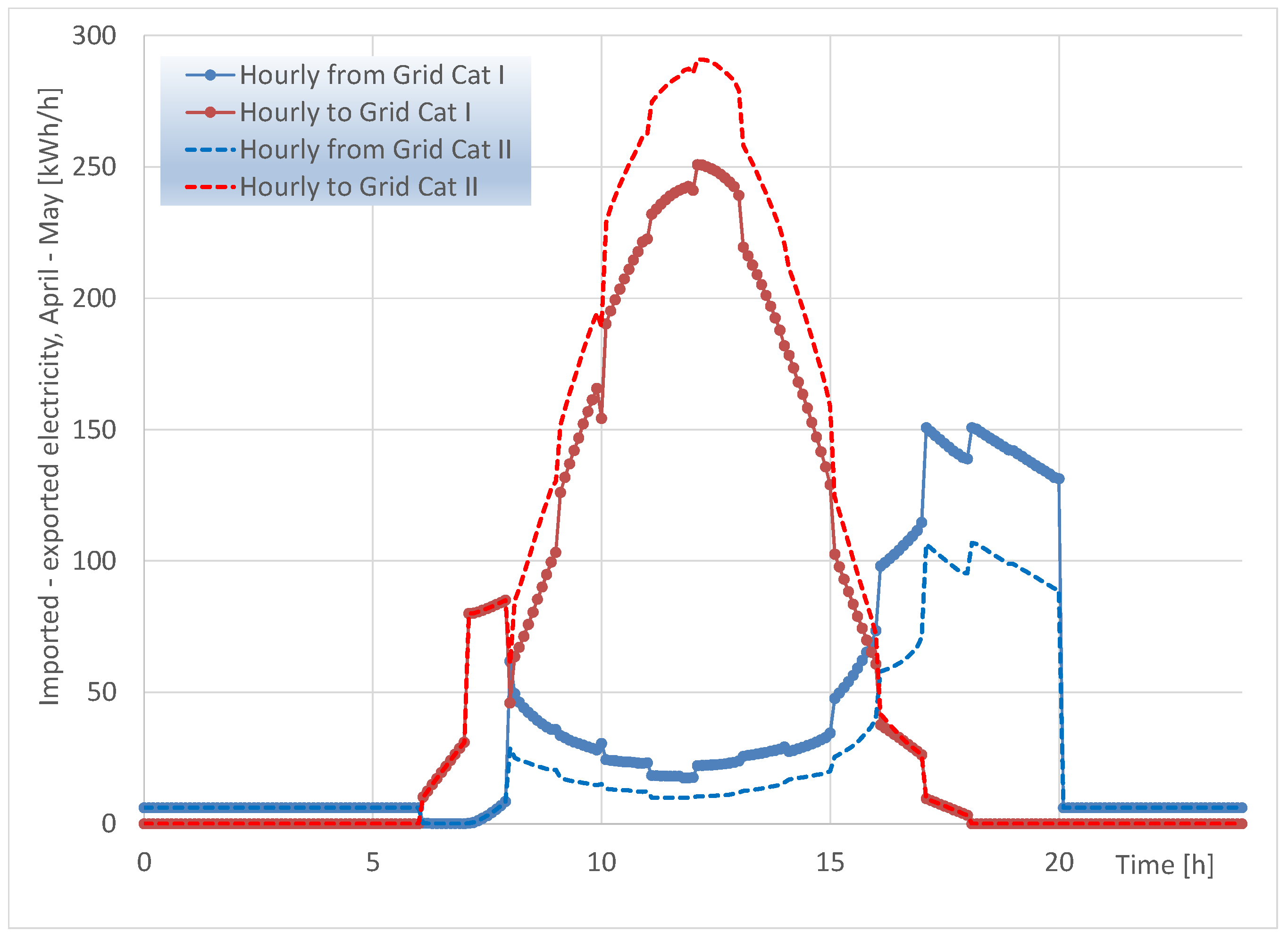
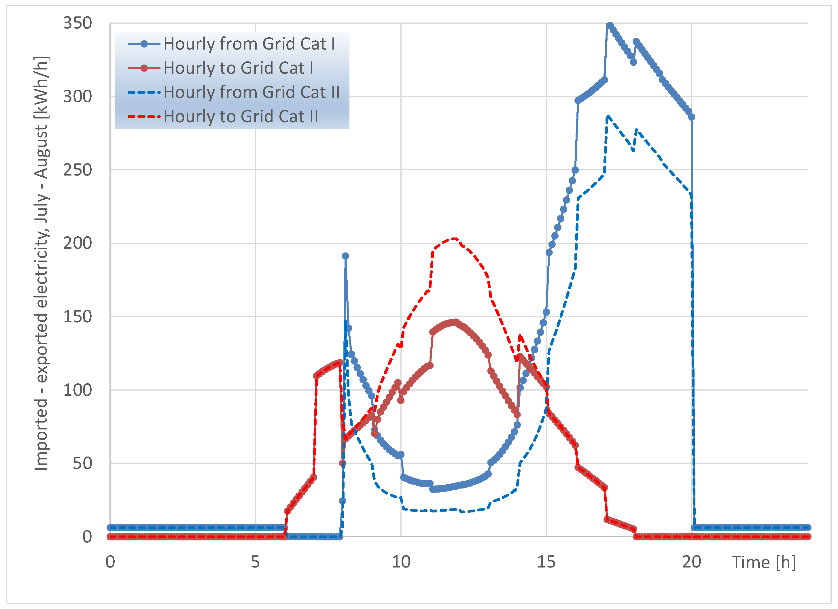
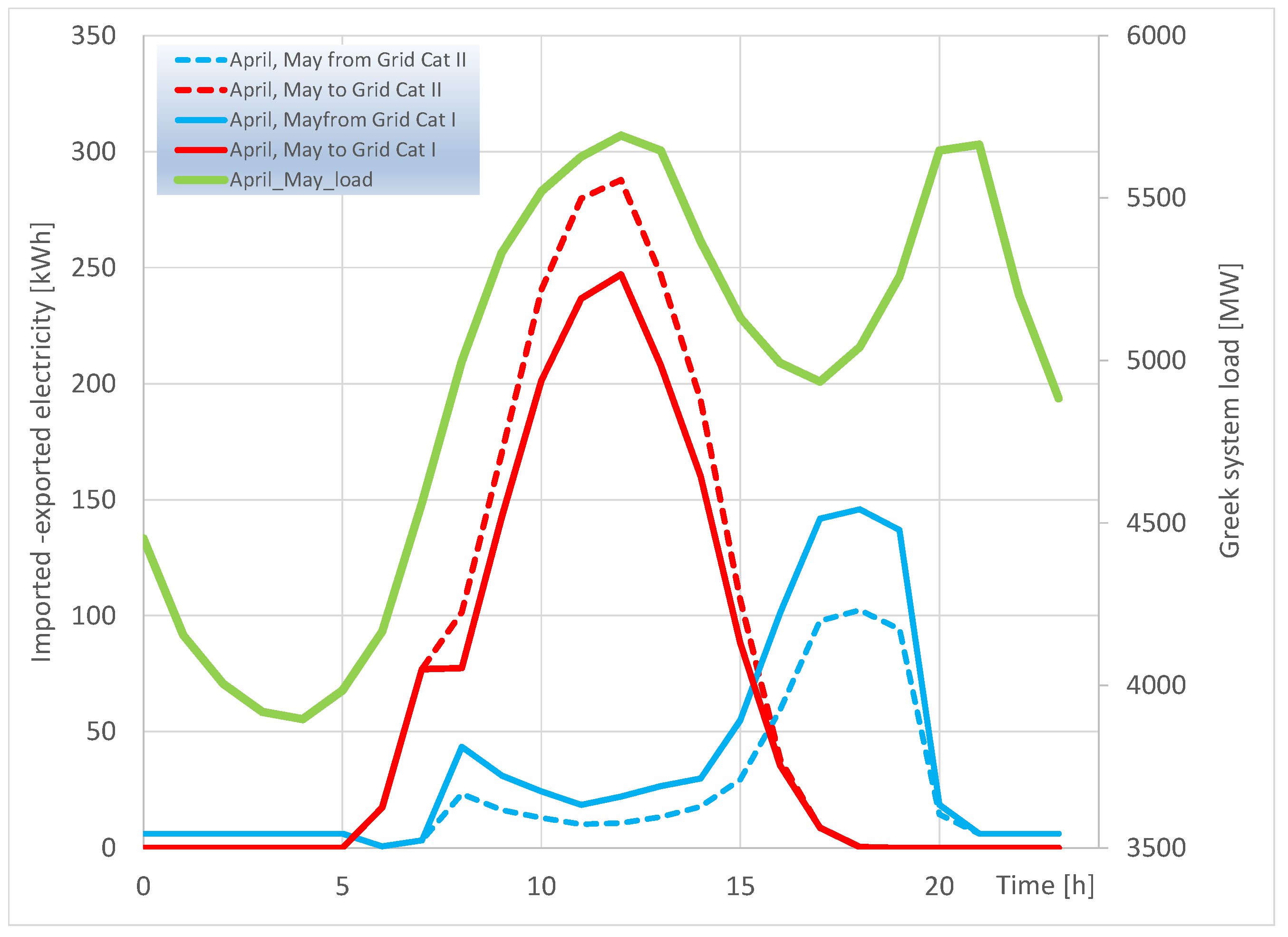
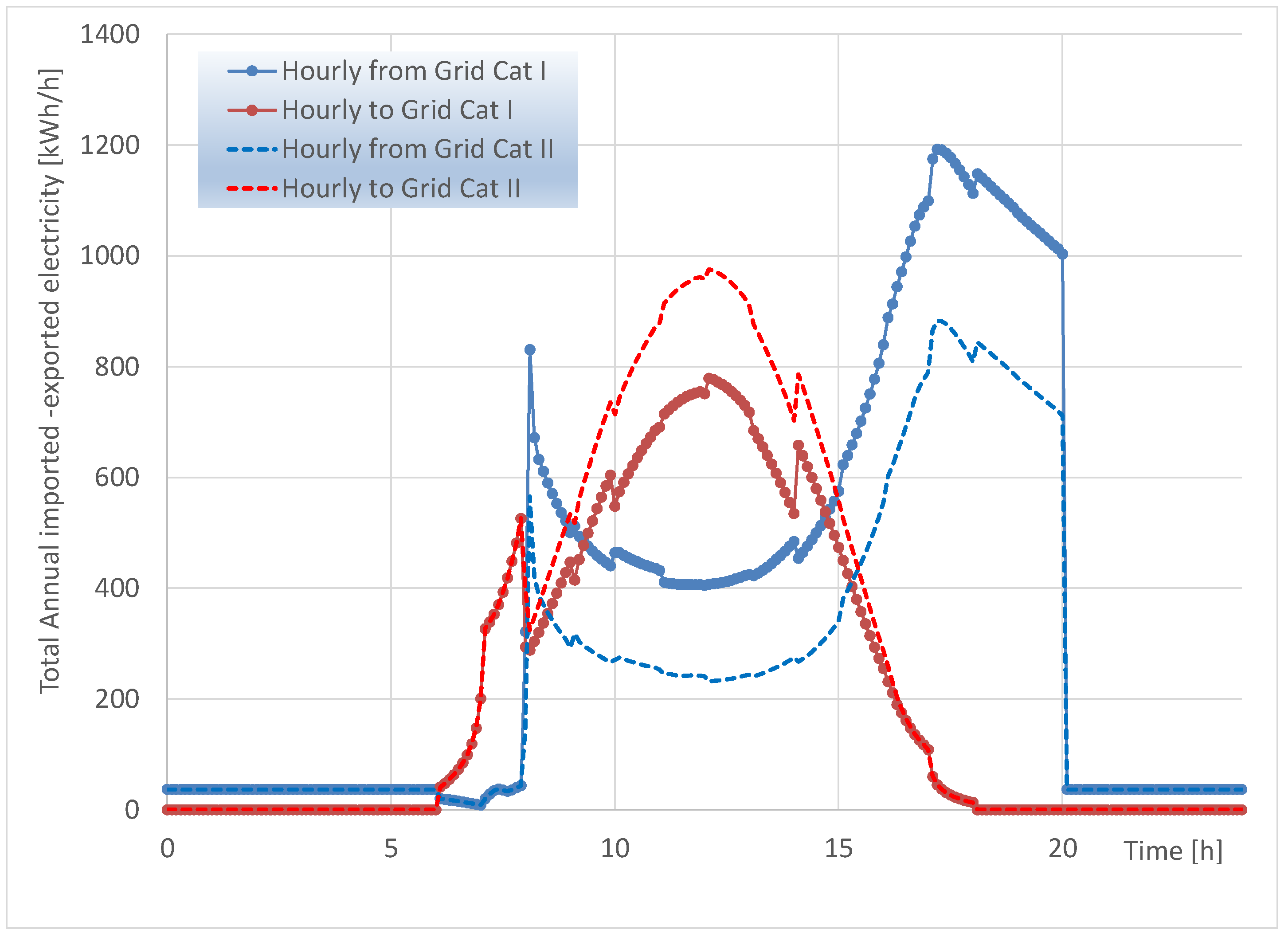
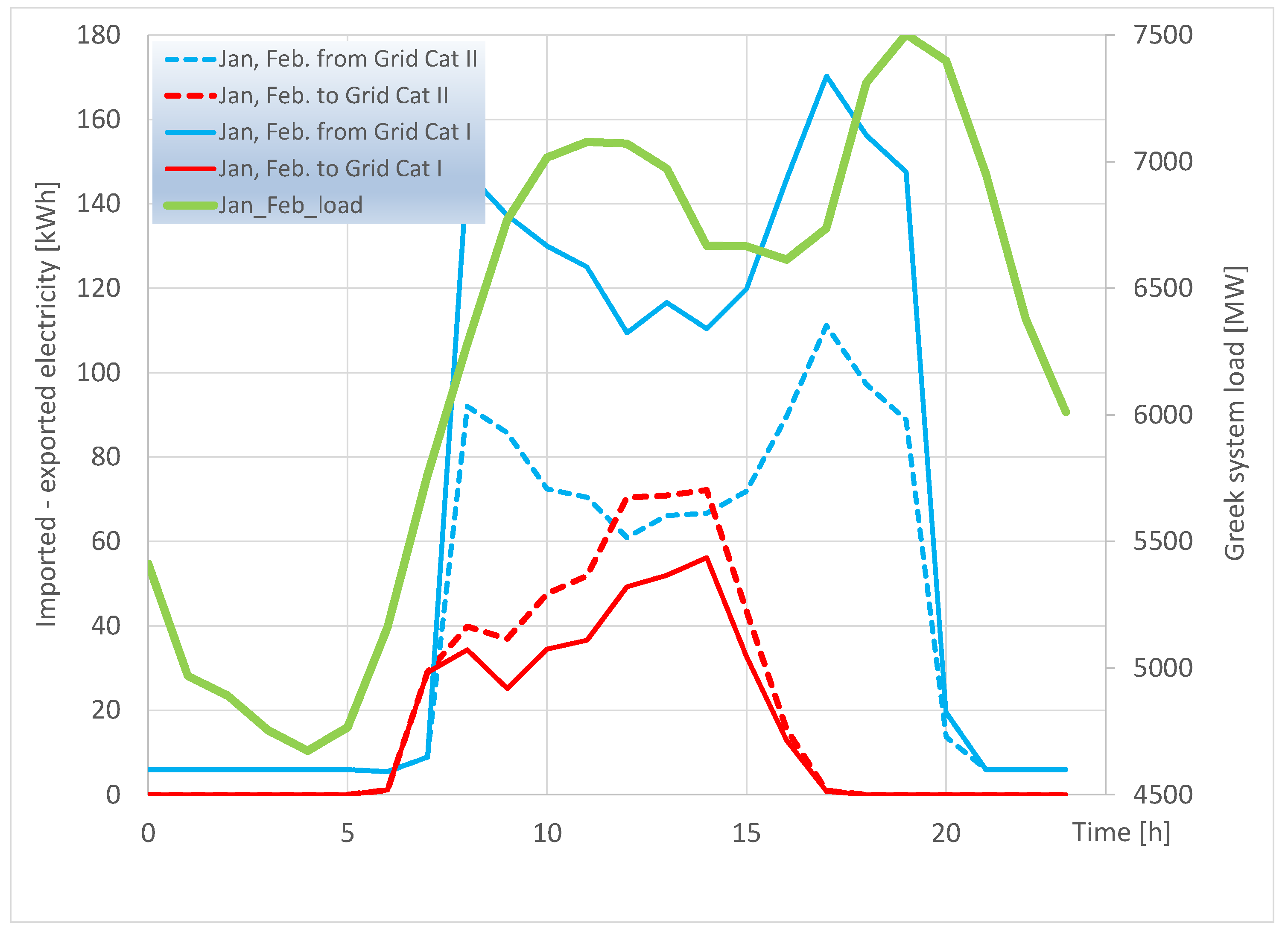
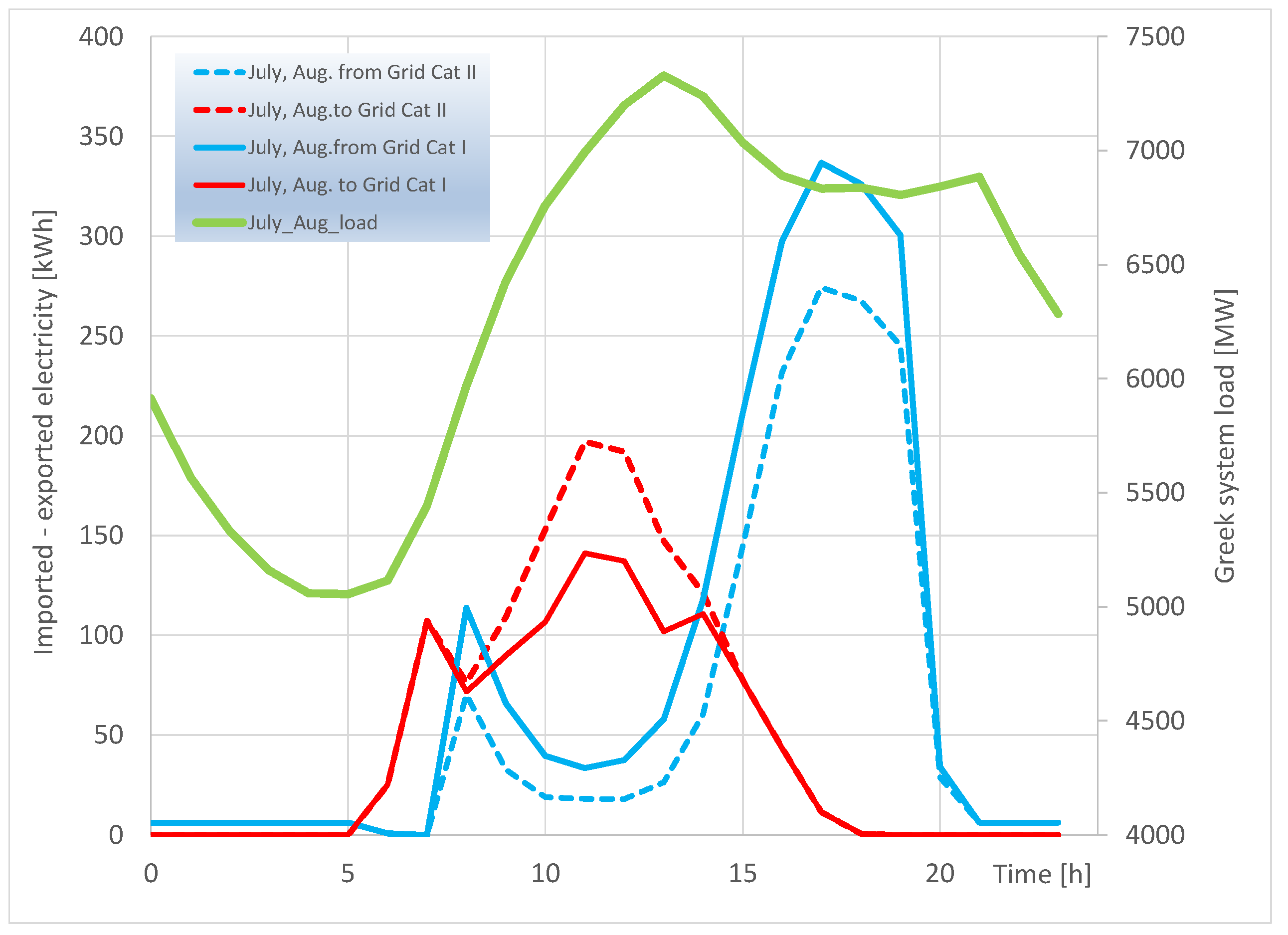
3.3. Comparative Performance of the Building with Category I–II Ventilation Requirements

A better assessment of the electricity exchange with the grid, according to the two alternative scenarios with the Category I–II requirements on the ventilation air quantities, can be seen in the diagram of Figure 15, with the total electricity from grid and the respective export to the grid plotted for each hour of the day. Starting from the standard category II requirements, we observe total exports of 400 kWh per hour at early morning hours 07:00–08:00 before the start of the working schedule. After 08:00, the situation reverses and we observe, during a significant number of days, a total demand for electricity import which sum up to 250–400 kWh/h, according to the Category II requirements, until 15:00 in the early afternoon. These total import quantities increase to the levels of 400–600 kWh/h when the simulations are carried out according to Category I ventilation requirements. On the other hand, presumably during a significant number of days in different seasons, electricity exports to the grid reaching 1000 kWh/h at noon hours for Category II ventilation (800 kWh/h for Category I) are observed. These stay above 600 kWh/h until 15:00 and continue decaying until 17:30. On the other hand, significant electricity imports are observed, presumably during different seasons during the same period. The total imports peak at 850 kWh/h for Category II and 1200 kWh/h for Category I requirements at 17:30, but they stay at high levels, above 700 and 1000 kWh/h, respectively, until the end of the daily working schedule, which takes place at 20:00 (Figure 14).

In order to understand the reasons for the observed seasonality in the behavior of the hourly electricity exchange of the building with the grid, under the two alternative scenarios of ventilation requirements, it is interesting to focus first on the situation during the cold winter months, January and February. This is presented in Figure 16, where, for Category II ventilation requirements, the total levels of electricity exported roughly match (with the exception of the early morning hours) the respective imports until 15:00 h. Afterwards, presumably due to the drop in PV production in this winter season, there are no more exports observed. The respective total electricity imports stay at an average of 100 kWh/h for Cat. II and 150 kWh/h for Cat. I requirements.

Thus, the changes from Category II to Category I requirements become especially apparent in the comparative plot of Figure 14, with regard to the total imported electricity from the grid, to cover the increased ventilation fans’ consumption.

Next, it is interesting to study the respective hourly distribution of electricity exchange with the grid during the neutral months of April-May. It can be observed in Figure 17 that the necessary imports are negligible until 15:00, presumably due to the negligible consumption of the heat pump and the available sunshine. On the other hand, the total electricity exported to the grid during this period reaches noon peak levels of 300 and 250 kWh/h for Cat II and I requirements, respectively. Afterwards, the situation is reversed and electricity imports peaking at 100 and 150 kWh/h are necessary until 20:00, according to Cat. II and Cat. I requirements, respectively.

Finally, it is interesting to focus on the behavior of the hourly electricity exchange with the grid during the hot summer months of July and August, where the heat pump consumption is at its highest levels, as is the PV electricity production. As seen in Figure 18, according to the Category II ventilation requirements scenario, the hourly balance of electricity exchange shows a prevailing export character until 15:00 h, since the necessary imports after a short peak between 08:00–09:00 become negligible until 14:00. On the other hand, from 15:00–20:00 h, we observe a quite significant increase of electricity imports that are necessary to cover the high consumption levels of the heat pump during the afternoon. Thus, electricity imports peaking at 280 and 350 kWh/h are necessary until 20:00, according to Cat. II and Cat. I requirements, respectively.

The above hourly results reveal two critical time slots where the building requests significant electricity quantities from the grid, especially with Category II ventilation requirements. The first is of very short duration, between 08:00–09:00, during the beginning of the work schedule. However, the second is of several hours duration and may significantly add to the stress of the external grid, which is already loaded during the afternoon ramp. As regards the available electricity surplus, due to its timing in the morning and noon hours, it is especially favorable to be allocated to charging the electric cars of employees which are parked in the available charging lots.

To summarize the system’s performance during the three different seasons, we start at Figure 19 with the two-months winter period. The increased requirements for electricity imports from the grid, according to Category I, between 09:00–10:00 a.m., coincide with the morning ramp of the Greek system’s load curve. The same observation is valid for the time slot 16:00–19:00, where the demand for imports is maximized, coinciding with the afternoon ramp of the Greek system’s load curve. The significant additional burden to the system, produced by the shifting from the standard category II requirements to the increased Category I, is obvious.

Continuing in Figure 20, with the neutral period of April—May, we observe, contrary to the previous period, that the building has available electricity surplus for export or charging of electric vehicles, almost coinciding with the morning ramp of the system’s load curve from the grid, between 08:00–11:00 am. That is, the building’s export capacity is favorable to address the needs of the external grid, both for Category I and Category II requirements. The situation reverses after 15:00, where a small demand for imports is observed. However, this demand ceases after 19:00, where the late afternoon ramp of the Greek system’s load is observed.

Finally, the situation changes again during the hot summer period of July–August, as seen in Figure 21. Only minimal requirements of short duration for electricity imports from the grid, according to Category I, are observed in the early morning, following a previous availability for export between 6:00–7:00. Thus, the morning ramp of the Greek system’s load curve (7:00–12:00) is not affected. On the contrary, a moderate export availability coincides with the morning ramp from 08:00–12:00. However, requirements for electricity import from the grid are maximized between 15:00–20:00, thus challenging the afternoon ramp of the demand curve. The significant additional burden to the system that is produced by the shifting from the standard category II requirements to the increased Category I is obvious also in this case.

As a next step, it would be interesting to study optimal regulation rules for on-demand ventilation to be operated in the specific type of building, or to examine alternate strategies to reduce the requirements of mechanical ventilation in office spaces that have ample access to external windows. Another important issue is the design optimization of the placement of inlet and exhaust grilles in each room or office space, aiming to realize displacement ventilation [44]. This ventilation technique has been proven most effective against virus transmission, initially studied in detail and supported by detailed measurements for the design of inpatient wards [45]. Finally, the additional burden placed by high-performance HEPA filters on the sizing of the ventilation system fans and the total electricity consumption is a matter of special importance for the future.

4. Conclusions

This paper examines in detail the additional burden to the ventilation system that is placed by the post-COVID-19 era, in a case study with an nZEB office building in Volos, Greece. The reference ventilation system design based on the existing standards EN 16798-1:2019 requires, according to the detailed calculations, the capability to supply a maximum of 19,000 m³/h outdoor air for Category II, which is the normal level adopted in new buildings and renovations. On the other hand, a good estimate of the added burden to the ventilation system is made by assuming the increased outdoor air requirements of Category I buildings of the same standard, with a high level of expectation for indoor air quality which are recommended for spaces occupied by very sensitive and fragile persons with special requirements. By adhering to these assumptions, the detailed calculations show that the system must be capable of supplying a maximum of 27,000 m³/h of outdoor air to the building. The comparative building energy simulation results of the alternative scenarios indicate an increase in the ventilation fans’ annual electricity consumption from 33,600 to 70,000 kWh. As a result of this increase, and, as the associated increase in the ventilation heating and cooling loads increase, the building shifts from a net electricity exporter of 4100 kWh (difference between exports and imports from the grid), to a net importer of 35,500 kWh per year, according to the worst-case scenario. This amounts to 18 kWh/m²y of net primary energy, a figure that challenges the nZEB character of the building. The increased electricity consumption of the Category I ventilation rates reduces electricity quantities that otherwise would be profitably available for charging the employees’ electric vehicles during the morning. As a means to reduce added costs, the oversized equipment could be operated in a demand-driven ventilation mode, which means that, during the normal operation (outside of COVID-19 episodes), the ventilator motors would be regulated at a reduced speed by their inverters. Also, the effect of advanced HEPA and electrostatic filters to the electricity consumption of the ventilation system needs to be carefully assessed and optimized in future research work.

References

1. European_Commission. Nearly Zero-Energy Buildings. 2022. Available online: https://energy.ec.europa.eu/topics/energy-efficiency/energy-efficient-buildings/nearly-zero-energy-buildings_en (accessed on 30 January 2023).
2. EU. Directive 2010/31/EU of the European Parliament and of the Council of 19 May 2010 on the Energy Performance of Buildings; EU: Maastricht, The Netherlands, 2010. [Google Scholar]
3. BPIE. Nearly Zero: A Review of EU Member State Implementation of New Build Requirements; BPIE: Brussels, Belgium, 2021. [Google Scholar]
4. Lebrouhi, B.E.; Schall, E.; Lamrani, B.; Chaibi, Y.; Kousksou, T. Energy Transition in France. Sustainability 2022, 14, 5818. [Google Scholar] [CrossRef]
5. Bottarelli, M.; González Gallero, F.J. Energy Analysis of a Dual-Source Heat Pump Coupled with Phase Change Materials. Energies 2020, 13, 2933. [Google Scholar] [CrossRef]
6. Stamatellos, G.; Zogou, O.; Stamatelos, A. Energy Analysis of a NZEB Office Building with Rooftop PV Installation: Exploitation of the Employees’ Electric Vehicles Battery Storage. Energies 2022, 15, 6206. [Google Scholar] [CrossRef]
7. Stamatellos, G.; Zogou, O.; Stamatelos, A. Interaction of a House’s Rooftop PV System with an Electric Vehicle’s Battery Storage and Air Source Heat Pump. Solar 2022, 2, 186–214. [Google Scholar] [CrossRef]
8. NN. ANSI/ASHRAE Standard 62.1-2004; Ventilation and Acceptable Indoor Air Quality: Atlanta, GA, USA, 2004; p. 44. [Google Scholar]
9. ANSI/ASHRAE. ASHRAE Standard 62.1-2022; Ventilation and Acceptable Indoor Air Quality (ANSI Approved): Atlanta, GA, USA, 2022. [Google Scholar]
10. ASHRAE. ASHRAE 62.1-2022 Document History. 2022. Available online: https://www.techstreet.com/ashrae/standards/ashrae-62-1-2022?product_id=2501063 (accessed on 30 January 2023).
11. Mokhtari, R.; Jahangir, M.H. The effect of occupant distribution on energy consumption and COVID-19 infection in buildings: A case study of university building. Build. Environ. 2021, 190, 107561. [Google Scholar] [CrossRef] [PubMed]
12. Lu, J.; Gu, J.; Li, K.; Xu, C.; Su, W.; Lai, Z.; Zhou, D.; Yu, C.; Xu, B.; Yang, Z. COVID-19 Outbreak Associated with Air Conditioning in Restaurant, Guangzhou, China, 2020. Emerg. Infect. Dis. J. 2020, 26, 1628. [Google Scholar] [CrossRef]
13. Dao, H.T.; Kim, K.-S. Behavior of cough droplets emitted from Covid-19 patient in hospital isolation room with different ventilation configurations. Build. Environ. 2022, 209, 108649. [Google Scholar] [CrossRef]
14. Xie, X.; Li, Y.; Chwang, A.T.Y.; Ho, P.L.; Seto, W.H. How far droplets can move in indoor environments–revisiting the Wells evaporation–falling curve. Indoor Air 2007, 17, 211–225. [Google Scholar] [CrossRef]
15. Guo, M.; Xu, P.; Xiao, T.; He, R.; Dai, M.; Miller, S.L. Review and comparison of HVAC operation guidelines in different countries during the COVID-19 pandemic. Build. Environ. 2021, 187, 107368. [Google Scholar] [CrossRef]
16. AE. AE-A-Series EV Charger. Available online: https://www.ae-electronics.com/ (accessed on 30 January 2023).
17. Hamdani, H.; Sabri, F.S.; Harapan, H.; Syukri, M.; Razali, R.; Kurniawan, R.; Irwansyah, I.; Sofyan, S.E.; Mahlia, T.M.I.; Rizal, S. HVAC Control Systems for a Negative Air Pressure Isolation Room and Its Performance. Sustainability 2022, 14, 11537. [Google Scholar] [CrossRef]
18. Zheng, W.; Hu, J.; Wang, Z.; Li, J.; Fu, Z.; Li, H.; Jurasz, J.; Chou, S.K.; Yan, J. COVID-19 Impact on Operation and Energy Consumption of Heating, Ventilation and Air-Conditioning (HVAC) Systems. Adv. Appl. Energy 2021, 3, 31. [Google Scholar] [CrossRef]
19. Alonso, A.; Llanos, J.; Escandón, R.; Sendra, J.J. Effects of the COVID-19 Pandemic on Indoor Air Quality and Thermal Comfort of Primary Schools in Winter in a Mediterranean Climate. Sustainability 2021, 13, 2699. [Google Scholar] [CrossRef]
20. Fageha, M.K.; Alaidroos, A.; Fageha, M.K.; Alaidroos, A. Performance Optimization of Natural Ventilation in Classrooms to Minimize the Probability of Viral Infection and Reduce Draught Risk. Sustainability 2022, 14, 14966. [Google Scholar] [CrossRef]
21. Sha, H.; Zhang, X.; Qi, D. Optimal control of high-rise building mechanical ventilation system for achieving low risk of COVID-19 transmission and ventilative cooling. Sustain. Cities Soc. 2021, 74, 103256. [Google Scholar] [CrossRef]
22. Wang, J.; Huang, J.; Feng, Z.; Cao, S.-J.; Haghighat, F. Occupant-density-detection based energy efficient ventilation system: Prevention of infection transmission. Energy Build. 2021, 240, 110883. [Google Scholar] [CrossRef]
23. EPA. Ventilation and Coronavirus (COVID-19). 2022. Available online: https://www.epa.gov/coronavirus/ventilation-and-coronavirus-covid-19 (accessed on 30 January 2023).
24. Mohammadi, M.; Calautit, J.; Mohammadi, M.; Calautit, J. Impact of Ventilation Strategy on the Transmission of Outdoor Pollutants into Indoor Environment Using CFD. Sustainability 2021, 13, 10343. [Google Scholar] [CrossRef]
25. Pampati, S.; Rasberry, C.N.; McConnell, L. Ventilation Impriesovement Strategies among K–12 Public Schools—The National School COVID-19 Prevention Stud. MMWR Morb. Mortal. Wkly. Rep. 2022, 71, 770. [Google Scholar] [CrossRef] [PubMed]
26. Marotta, A.; Porras-Amores, C.; Rodríguez Sánchez, A. Resilient Built Environment: Critical Review of the Strategies Released by the Sustainability Rating Systems in Response to the COVID-19 Pandemic. Sustainability 2021, 13, 11164. [Google Scholar] [CrossRef]
27. REHVA. Health-based target ventilation rates and design method for reducing exposure to airborne respiratory infectious diseases. In REHVA Proposal for Post COVID Target Ventilation Rates; REHVA: Brussels, Belgium, 2022. [Google Scholar]
28. EN 16798-1:2019; Energy Performance of Buildings-Ventilation for Buildings-Part 1: Indoor Environmental Input Parameters for Design and Assessment of Energy Performance of Buildings Addressing Indoor Air Quality, Thermal Environment, Lighting and Acoustics. CEN: Brussels, Belgium, 2019.
29. Stamatellos, G.; Zogou, O.; Stamatelos, A. Energy Performance Optimization of a House with Grid-Connected Rooftop PV Installation and Air Source Heat Pump. Energies 2021, 14, 740. [Google Scholar] [CrossRef]
30. Zogou, O.; Stamatelos, A. Optimization of thermal performance of a building with ground source heat pump system. Energy Convers. Manag. 2007, 48, 2853–2863. [Google Scholar] [CrossRef]
31. Zogou, O.; Stamatelos, A. Application of Building Energy Simulation in the Sizing and Design Optimization of an Office Building and Its HVAC Equipment; Chapter 11 in Energy and Buildings: Efficiency, Air Quality, and Conservation; Utrick, J.B., Ed.; Nova Science Publishers: Hauppauge, NY, USA, 2009. [Google Scholar]
32. Safa, A.A.; Fung, A.S.; Kumar, R. Heating and cooling performance characterisation of ground source heat pump system by testing and TRNSYS simulation. Renew. Energy 2015, 83, 565–575. [Google Scholar] [CrossRef]
33. Neymark, J.; Judkoff, R.; Knabec, G.; Lec, H.-T.; Duerig, M.; Glasse, A.; Zweifele, G. Applying the building energy simulation test (BESTEST) diagnostic method to verification of space conditioning equipment models used in whole-building energy simulation programs. Energy Build. 2002, 34, 917–931. [Google Scholar] [CrossRef]
34. Standard 140-2001; Standard Method of Test for the Evaluation of Building Energy Analysis Computer Programs. ASHRAE: Atlanta, GA, USA, 2001.
35. Component Libraries for TRNSYS, Version 2.0. User’s Manual; TESS: Madison, WI, USA, 2004; Available online: http://www.tess-inc.com/services/software (accessed on 30 January 2023).
36. S&P. EasyVent Fan Selection Tool. Available online: https://easyvent.solerpalau.com/ (accessed on 30 January 2023).
37. De Soto, W.; Klein, S.A.; Beckman, W.A. Improvement and validation of a model for photovoltaic array performance. Sol. Energy 2006, 80, 78–88. [Google Scholar] [CrossRef]
38. Sharp. 415Wp/Mono NUJC415 Data Sheet. Available online: https://docs.aws.sharp.eu/Marketing/Datasheet/2208_NUJC_415_HC-Mono_Datasheet_EN.pdf (accessed on 30 January 2023).
39. Chen, C.-Y.; Chen, P.-H.; Chen, J.-K.; Su, T.-C. Recommendations for ventilation of indoor spaces to reduce COVID-19 transmission. J. Formos. Med. Assoc. 2021, 120, 2055–2060. [Google Scholar] [CrossRef]
40. EU. COMMISSION RECOMMENDATION (EU) 2016/1318 of 29 July 2016 on Guidelines for the Promotion of Nearly Zero-Energy Buildings and Best Practices to Ensure That, by 2020, All New Buildings Are Nearly Zero-Energy Buildings; Official Journal of the European Union: Brussels, Belgium, 2016. [Google Scholar]
41. Sang, J.; Liu, X.; Liang, C.; Feng, G.; Li, Z.; Wu, X.; Song, M. Differences between design expectations and actual operation of ground source heat pumps for green buildings in the cold region of Northern China. Energy 2022, 252, 124077. [Google Scholar] [CrossRef]
42. Huang, S.; Zhu, K.; Dong, J.; Li, J.; Kong, W.; Jiang, Y.; Fang, Z. Heat transfer performance of deep borehole heat exchanger with different operation modes. Renew. Energy 2022, 193, 645–656. [Google Scholar] [CrossRef]
43. Wang, Y.; Wang, Y.; You, S.; Zheng, X.; Wei, S. Operation optimization of the coaxial deep borehole heat exchanger coupled with ground source heat pump for building heating. Appl. Therm. Eng. 2022, 213, 118656. [Google Scholar] [CrossRef]
44. Awbi, H. Ventilation Systems: Design and Performance; Taylor and Francis: Abingdon, UK, 2008. [Google Scholar]
45. Ren, J.; Wang, Y.; Liu, Q.; Liu, Y. Numerical Study of Three Ventilation Strategies in a prefabricated COVID-19 inpatient ward. Build. Environ. 2021, 188, 107467. [Google Scholar] [CrossRef]
Figure 1. Layout drawing of the office building employed in the simulations: (a) Plan of a typical floor level, (b) plan of rooftop PV installation and rooftop air-handling units. Dimensions in meters (m).
Sustainability 15 03422 g001
Figure 2. Schematic of a typical ventilation system.
Sustainability 15 03422 g002
Figure 3. Characteristic performance curves and design operation points of the two types of supply fans installed in the respective air-handling units (a) 1.1 kW, 3-phase, 4-pole motor, direct-drive; (b) 0.55 kW, 3-phase, 4-pole motor, direct-drive [36].
Sustainability 15 03422 g003
Figure 4. Typical pre-filter (left) and bag filter (right) installed at the supply side of the Air-handling Units (see Figure 2).
Sustainability 15 03422 g004
Figure 5. Schematic of TRNSYS-16 building energy system’s model, with all types employed in the simulation studio.
Sustainability 15 03422 g005
Figure 6. Characteristic performance curves and design operation points of the two types of supply fans installed in the respective air-handling units (a) 2.2 kW, 3-phase, 4-pole motor, direct-drive; (b) 1.1 kW, 3-phase, 4-pole motor, direct-drive [36].
Sustainability 15 03422 g006
Figure 7. Monthly electricity production and consumption during the year.
Sustainability 15 03422 g007
Figure 8. Heat pump energy performance and electricity consumption on a monthly basis. Heat gain from the ground and heat transferred to the load are positive in heating mode and negative in cooling mode. Cooling mode prevails between May—October, as seen by the negative thermal kWh values.
Sustainability 15 03422 g008
Figure 9. Monthly quantities of PV production and main types of electricity consumption of the office building with category II ventilation.
Sustainability 15 03422 g009
Figure 10. Ambient temperature, zone 1 temperature, heat pump consumption, PV inverter out power, and ventilation fan consumption during the second week of January.
Sustainability 15 03422 g010
Figure 11. Transient building’s energy performance during a week in the beginning of May. Cooling season temperature set point is 25 °C.
Sustainability 15 03422 g011
Figure 12. Transient building’s energy performance during one week in late June with a heat-wave. Temperature set point to 25 °C.
Sustainability 15 03422 g012
Figure 13. Power levels that are imported or exported hourly to the electricity grid in the course of the year.
Sustainability 15 03422 g013
Figure 14. Monthly quantities of PV electricity production and electricity consumption of the building with Category I ventilation.
Sustainability 15 03422 g014
Figure 15. Total electricity imported—exported to the grid for each hour of the day: Comparison of Category I versus Category II indoor air quality requirements.
Sustainability 15 03422 g015
Figure 16. Total hourly imported—exported electricity during the two-month period 1.1–28.2: Comparison of Category I versus Category II indoor air quality requirements.
Sustainability 15 03422 g016
Figure 17. Total hourly imported—exported electricity during the two-month period 1.4-31.5: Comparison of Category I versus Category II indoor air quality requirements.
Sustainability 15 03422 g017
Figure 18. Total hourly imported—exported electricity during the two-month period 1.7–31.8: Comparison of Category I versus Category II indoor air quality requirements.
Sustainability 15 03422 g018
Figure 19. Correlation of the hourly imported—exported electricity during the two-month period 1.1–28.2, with the average hourly Greek system’s load for the same period. Category I versus Category II indoor air quality requirements.
Sustainability 15 03422 g019
Figure 20. Correlation of the hourly imported—exported electricity during the neutral two-month period 1.4–31.5, with the average hourly Greek system’s load for the same period. Category I versus Category II indoor air quality requirements.
Sustainability 15 03422 g020
Figure 21. Correlation of the hourly imported—exported electricity during the hot summer period 1.7–31.8, with the average hourly Greek system’s load for the same period. Category I versus Category II indoor air quality requirements.
Sustainability 15 03422 g021