Comprehensive Review on Waste Generation Modeling

Abstract

Strategic plans for waste management require information on the current and future waste generation as a primary data source. Over the years, various approaches and methods for waste generation modeling have been presented and applied. This review provides a summary of the tasks that require information on waste generation that are most frequently handled in waste management. It is hypothesized that there is not currently a modeling approach universally suitable for forecasting any fraction of waste. It is also hypothesized that most models do not allow for modeling different scenarios of future development. Almost 360 publications were examined in detail, and all of the tracked attributes are included in the supplementary. A general step-by-step guide to waste generation forecasting, comprising data preparation, pre-processing, processing, and post-processing, was proposed. The problems that occurred in the individual steps were specified, and the authors’ recommendations for their solution were provided. A forecasting approach based on a short time series is presented, due to insufficient options of approaches for this problem. An approach is presented for creating projections of waste generation depending on the expected system changes. Researchers and stakeholders can use this document as a supporting material when deciding on a suitable approach to waste generation modeling or waste management plans.

1. Introduction

In developing countries, the prevailing goal is to dispose of waste, while in developed countries (e.g., the ones in the EU), there is an effort to process the waste more sustainably. The preferred methods of waste management (WM) and disposal in the EU have been stipulated in the Waste Management Hierarchy [1] to make use of the waste potential. The EU member states have been implementing the necessary legislative changes, and the next step is to adapt the existing WM systems to meet the respective objectives. Strategic plans for the modernization and construction of waste collection and processing infrastructure require information on the generation and composition of waste, including their expected development, as a primary data source. The aim is to create a WM system that is sustainable from both the economic and environmental points of view. In response to this situation, there is a growing number of publications dealing with waste generation modeling. This review aims to summarize the available modeling approaches and discuss their suitability for different applications in WM.

1.1. Application-Based Targeting

WM is a very complex field in which many tasks and problems can be encountered in decision-making. The direction of WM development is conditioned by the appropriate strategic planning of the various components of the WM system (waste collection, construction of new treatment facilities, change in facility capacity). A whole series of interventions in the system requires several years for the preparation and implementation of the plan. It is therefore necessary to start from well-developed comprehensive strategic plans, which, among other things, take into account the expected development of the generation of the waste fractions in question.

Each task is unique in nature, but all stages of the process require specific input data, differing mainly in their time or territorial detail. The most challenging parameters are the generation rates of different types of waste and waste composition (mostly MMW or separately collected waste, e.g., paper, plastic). Therefore, the tasks are divided into three logical blocks, where their characteristics are described to create models associated with the current or future waste quantities.

1.1.1. Waste Management Legislation and Policy

The proper specification of the recycling or waste prevention targets included in legislation requires reliable long-term knowledge of waste generation and treatment. Historical data can identify the links of various socio-economic and demographic factors to WM development [2]. The connections identified may reveal potential societal changes and, consequently, positively affect waste generation trends and processing methods.

In the context of long-term forecasting (5–20 years), the Circular economy package of the EU is relevant because it sets recycling targets for municipal solid waste (MSW) until 2035 [3] and landfill restrictions [4]. At the country level, the data are usually aggregated annually, and as such, are suitable for forecasting. The disadvantage often is the availability of only short historical data series, due to annual data records. The only reasonable alternative for forecasting is finding the trend that the data follow (Section 4.3.2). Ghinea et al. (2016) [5] considered multiple functions for describing trends, of which the S-curve proved to be the most suitable for MSW. Ayeleru et al. (2018) [6] used a linear dependence to describe the expected city-level rate of the generation of MSW. Other available works dealt with very complex models that are not suitable for forecasting. A complete overview is given in the Supplementary Materials (see Section 2.1).

Modeling waste generation makes it possible to compare mostly very ambitious legislative goals with the forecasted values. The most significant shortcoming of the methods for the longer-term estimation of waste generation is the failure to consider potential interventions in the waste system itself. If the forecast is not in line with the goals, then the projections are modeled. This can reveal the potential for changes in individual territorial units. Within the projections, the forecasts are modified to achieve the set target [7].

1.1.2. Strategic Decision-Making on Waste Management Infrastructure

Strategic decision-making in WM concerns the planning and implementation of long-term projects for facility construction [8]. Compared to the previous part, waste management legislation and policy, waste generation forecasting usually focuses on the regional level. Data at the regional level are often available on an annual basis and estimating trends from historical data is possible. However, the data and trends also usually feature significant volatility, which makes forecasting more complicated and less accurate. It is good to keep in mind the conditions in the surrounding regions that may affect the planned project [9]. A hierarchical territorial division can ensure consistent forecasts between regions and the entire country [10]. The definition of possible scenarios for future waste amounts takes place in the strategic planning. Such scenarios arise from external interventions into the WM system, and they allow for evaluating the impact on the planned projects’ sustainability [11].

A significantly shorter time horizon is sufficient for collection strategy planning due to the relatively short service life of collection containers and frequent legislative changes [12]. Models for collection planning usually focus on the daily or weekly data sets. This type of data is common for cities and municipalities, where monitoring is conducted in greater detail and during longer time horizons.

To ensure the financial and technical sustainability of a project, it is necessary to assume, during its evaluation, that several parameters are uncertain, including the generation rate and the waste composition [13]. The current state and outlook for the area of interest are needed to appropriately site a new facility or collection infrastructure with a well-chosen capacity.

1.1.3. Operational Decision-Making in Waste Management

The last point is related to the planning of daily operations. Container level data are needed in waste collection applications that use routing models (a summary of routing problems and their application was presented by [14], which may feature various targets. A typical representative of this is dynamic collection planning, where the waste quantities at the individual collection points are estimated each day. On the other hand, when creating a new collection plan, weekly or monthly data are required to properly set the collection frequency. The frequency itself depends on both the waste properties and the capacities of the collection points. Collection planning is closely related to the siting of the collection points, which was discussed in detail in the previous sections.

1.2. Tasks Encountered in Waste Generation Modeling

When building waste generation models, it is necessary to distinguish whether an estimate of the current or the future generation rate is made. The differences in the terminology regarding prediction, forecasting, and projection are provided in the following sections.

1.2.1. Prediction

The prediction of waste generation is used to describe the current or future situation. Estimating the current waste generation rate is essential to define the links in the system and to develop the models for other territorial units. These links can be used to model the expected future waste generation. A common application is in the modeling of the waste generation rate, depending on various socio-economic, demographic, and other factors. The pitfalls of such models were described by [15] in more detail. The main weakness is that the links in the system can change over time. Problems may occur when the links are modeled using all of the historical data, without regard to their temporal variance. Consequently, this may impact the quality of the future predictions of the respective models.

A common mistake is also to build models using the absolute data, without standardization. Then, multicollinearity is often observed, which negatively impacts the obtained results. In addition, the data yielded by a WM model should always include information on the uncertainty, e.g., via confidence intervals.

1.2.2. Forecasting

Forecasting, sometimes termed prognosis, exclusively concerns the estimation of future development. Most forecasts in WM involve waste generation. Other forecasting targets (waste composition, waste treatment) are rare. When making a forecast, it is necessary to remember that inferring the future development based on the current or historical data is always a difficult—and often largely unsolvable—task.

Forecasting models assume that the respective parameters will evolve in a similar way to their past development. The primary feature of a forecast is that no change in the current conditions is expected. Data from even short-term forecasts must be evaluated carefully. Longer-term forecasts are more indicative in terms of how the development of waste generation might manifest if nothing changes (e.g., without any changes being made to the legislation). When it comes to waste generation, the problem is further compounded by the fact that often only data sets covering very short time ranges are available. If sociology-, economics-, or demography-related data from a “prediction” model are to be used, it is imperative that such a prediction is of sufficient quality.

Forecasts should also consider the links between the waste streams, which are interrelated (higher generation of separated waste leads to lower amount of mixed municipal waste (MMW) etc.). A model should always allocate a certain number of data points at the end of the time series for verification purposes. Even in forecasting, the results should include information on the uncertainty.

1.2.3. Projection

Projections also deal with the estimation of future development; however, in contrast to forecasting, they assume that a change will happen in the boundary conditions (legislative, technological progress). These conditions, which affect waste generation, cannot be forecasted. Therefore, projections are often future scenarios given the specific boundary conditions chosen by the authors. Scenarios can be created with respect to the objectives of the WM, but deviations from the corresponding forecast should be as slight as possible. Due to territorial hierarchy, it is appropriate to consider the division of national targets (i.e., individual regions according to their potential for change). Monotony in terms of waste generation potential should be maintained. Possible links among waste fractions should also be taken into account.

1.3. Research Questions

The underlying goal of this review is to gather supporting material for the development of a comprehensive waste generation model, particularly with regard to its application (see Section 1.1). Before studying the available literature, the research questions that are addressed in the following text are formulated.

• What are the common shortcomings of the available data, and how many data points in a time series are sufficient? Response: Section 2.1 and Section 3.
• Which approaches and methods are suitable for certain applications? Response: Section 3.
• Can general recommendations be formulated for data processing? Response: Section 4.
• Can prediction models be used to estimate future data? Under what conditions? Response: Section 5.
• How to implement changes and interventions in WM (legislative interventions, changes in data reporting methodology, introduction of new waste catalogue numbers) within mathematical models? Response: Section 5.

The actual review methodology is described in Section 2. A detailed overview of the studied publications can be found in Supplementary Materials. An extensive review was carried out in order to create an overview of the methods and approaches to date. Based on this, it is possible to choose a suitable approach for other tasks. In the event that the existing approaches are insufficient for some types of tasks, it is appropriate to consider the issue of developing new approaches. Section 3 presents the process of choosing a modeling method. Section 4 then summarizes the modeling processes (preparation, pre-processing, processing, post-processing) in the form of the problems and the authors’ recommendations. A SWOT analysis for the individual models is provided for each method in Appendix A. The main benefit of this contribution is the combined approach of forecasting and projection based on a short time series, see Section 5. The presented method is designed as a universal approach for any waste fraction. The lack of a multipurpose approach was found to be a research gap. A common and problematic feature of the available data is a short time series. Considering this feature, the approach is based on a trend analysis of the historical data, followed by data reconciliation. This choice took place according to the decision-making process in Section 3. A brief summary is provided in Section 6, including the suggestions regarding further research directions.

2. Literature Review

First, attention was paid to previously published review papers on the discussed topic, with the aim being to prevent repetition, the summary is in

Table 1. Previously published review papers.

Citation	Time Range	Number of Publications	Criteria
(Beigl et al., 2008 [16]);	Until 2005	45	regional scale, MSW waste streams, independent variables, modeling methods
(Cherian and Jacob, 2012 [17])	Until 2011	9	regional scale, MSW waste streams, independent variables, modeling methods, socio-economic factors
(Kolekar et al., 2016 [18])	2006–2014	20	modeling methods, territorial division, amount and frequency of time-dependent data, independent variables, waste stream
(Goel et al., 2017 [19])	1972–2016	106	classification into typical (multiple linear regression—MLR, time series analysis—TSA, factor analysis) and unconventional (fuzzy methods, artificial neural networks—ANN) approaches
(Alzamora et al., 2022 [20])	2008–2021	120	MSW stream, geographic scale, data type, modeling technique, independent variables
(Abdallah et al., 2020 [21])	2004–2019	85	artificial intelligence in WM, identified six applications; described multiple models incl. hybrid ones
(Guo et al., 2021 [22])	2003–2020	40	machine learning methods in organic solid waste treatment
(Xu et al., 2021 [23])	2010–2020	177	ANN models, categories of review scales: macroscale (mainly focused on waste generation), mesoscale (waste properties and process parameters), meso-microscale (waste process efficiencies), microscale (reaction mechanisms or microstructures)

.

Older reviews clearly specify the as-of-yet unresolved research gap, while the more recent works—e.g., [21,22,23]—deal exclusively with artificial intelligence and do not consider other methods. As the works by [17,18] described the target periods with only a modest number of published models, a new review for that period has been conducted in the present paper. The contribution [19] presented a relatively extensive review, but further applications require more elaboration in the context of waste fractions. The contribution [20] aims to investigate the relationship between waste generation and socioeconomic factors. Thus, a review of approaches that do not use influential factors for models (e.g., TSA) is not provided. Therefore, the review will be carried out again in this contribution, with a broader scope of the methods used. The review [16] is taken as the starting point, the publication is ca. 15 years old and, therefore, an update is due. The review [16] summarizes the methods used until 2005, but there are no described new approaches that have not been addressed until then. It is therefore not necessary to study the contributions before 2006, as this period has already been well covered in paper [16].

The review is therefore conducted for articles published in 2006 and later. The main databases queried were ScienceDirect and Scopus with the keywords being: “msw prediction“, “msw forecast“, “waste prediction“, “waste forecast“, “waste generation“, “waste production“, “waste forecasting“, “municipal waste prediction“ or “municipal waste forecast“. The articles were sort on “relevance”.

For the articles that matched the listed keywords, their relevance to this review was assessed against the title or abstract. The criterion is that the chosen article presents a model of either the current or future waste generation. When sorting by relevance, the articles suitable for review are first displayed. Then, more occurred, which were excluded from the review. When there were more than 20 non-relevant articles in a row when sorting by relevance, the search was terminated. A total of 359 articles were identified for the detailed examination within the review.

The following text is particularly beneficial because it contains detailed modeling recommendations for specific WM applications. The criteria utilized in [16] have been kept and several new parameters (the amount of data, waste types, etc.) have been added.

2.1. Summary of the Results

This study evaluated the 359 selected publications from several points of view. A detailed overview of all the monitored criteria is available in Supplementary Materials; the main text contains references only to the fundamental publications that the authors have chosen for the citation in individual parts of the text. Supplementary Materials is structured as follows:

• Publication details (columns B–H): title, authors, journal, year, nationality according to the affiliation of the main author, number of citations, keywords.
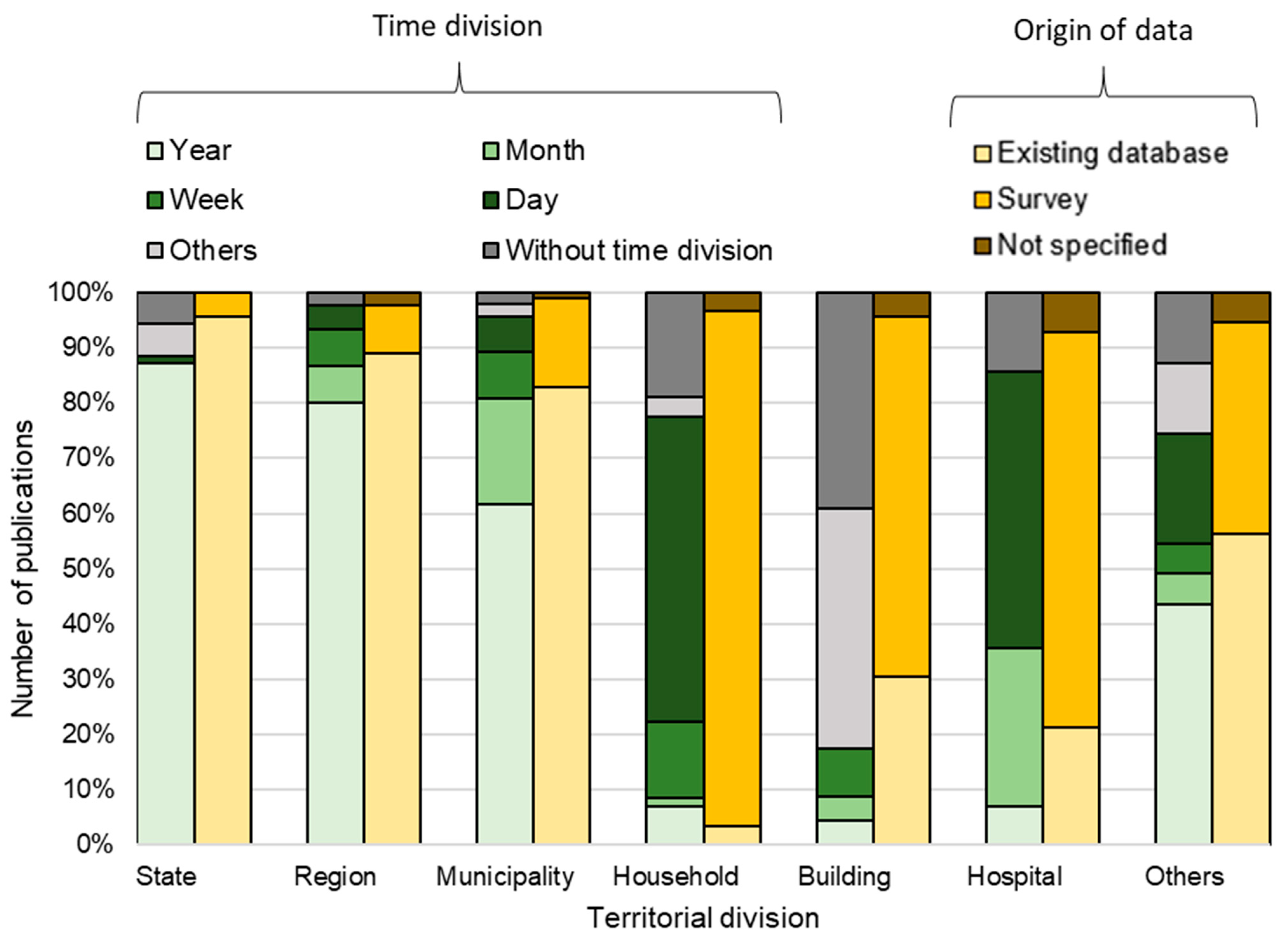
• Origin of data (columns I–K): state, continent, the source of WM data.
• Data details (columns L–R): number of dependent variables, time interval, number of time intervals, territorial division, number of territories.
• Forecasting (columns S, T): forecasting (yes/no), forecasting period length.
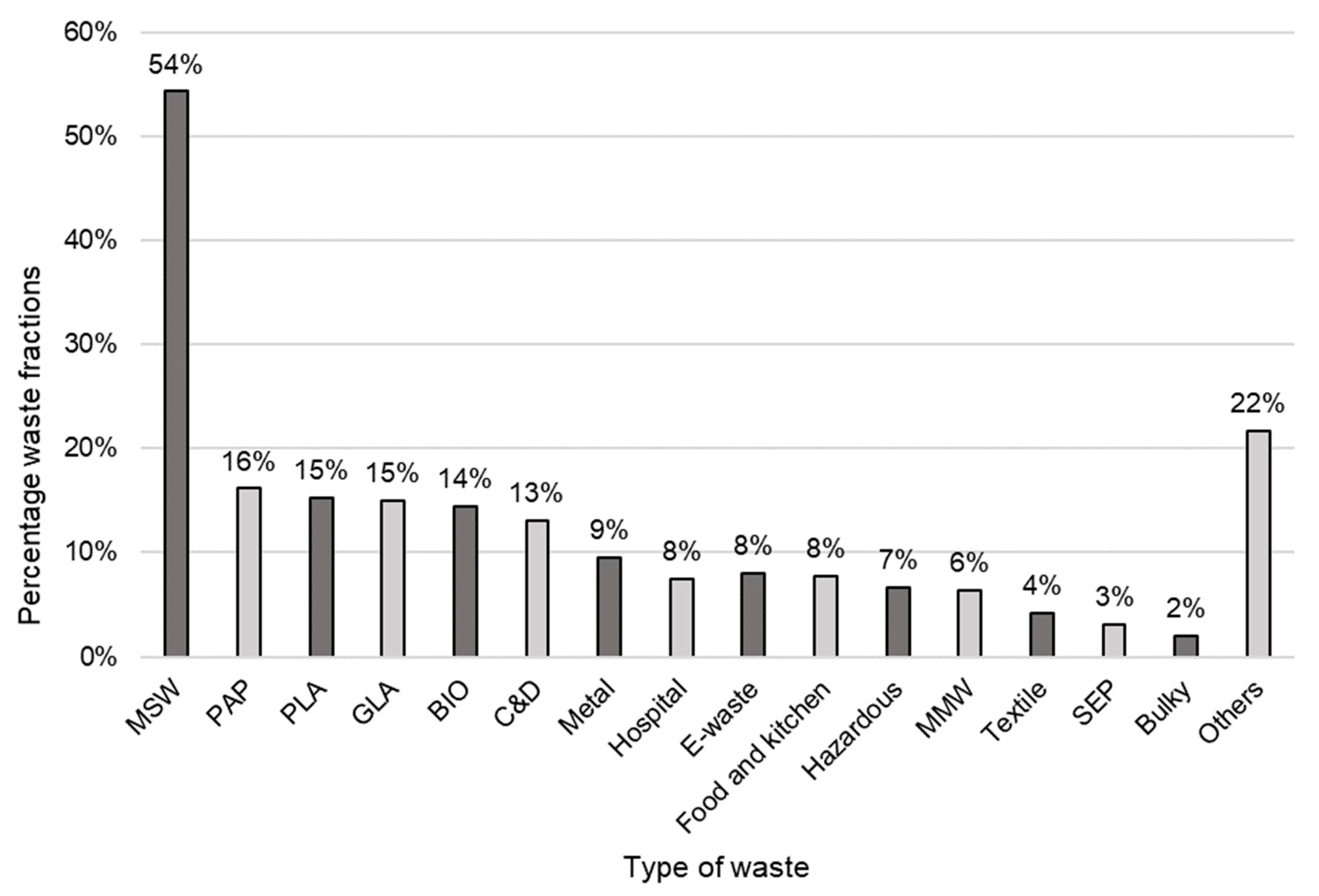
• Waste streams (columns U–AK): MSW, MMW, bio-waste, paper, plastics, glass, etc.
• Influencing factors (columns AL–AT): influencing factors (yes/no), population size, education, age, income, gross domestic product (GDP), etc.
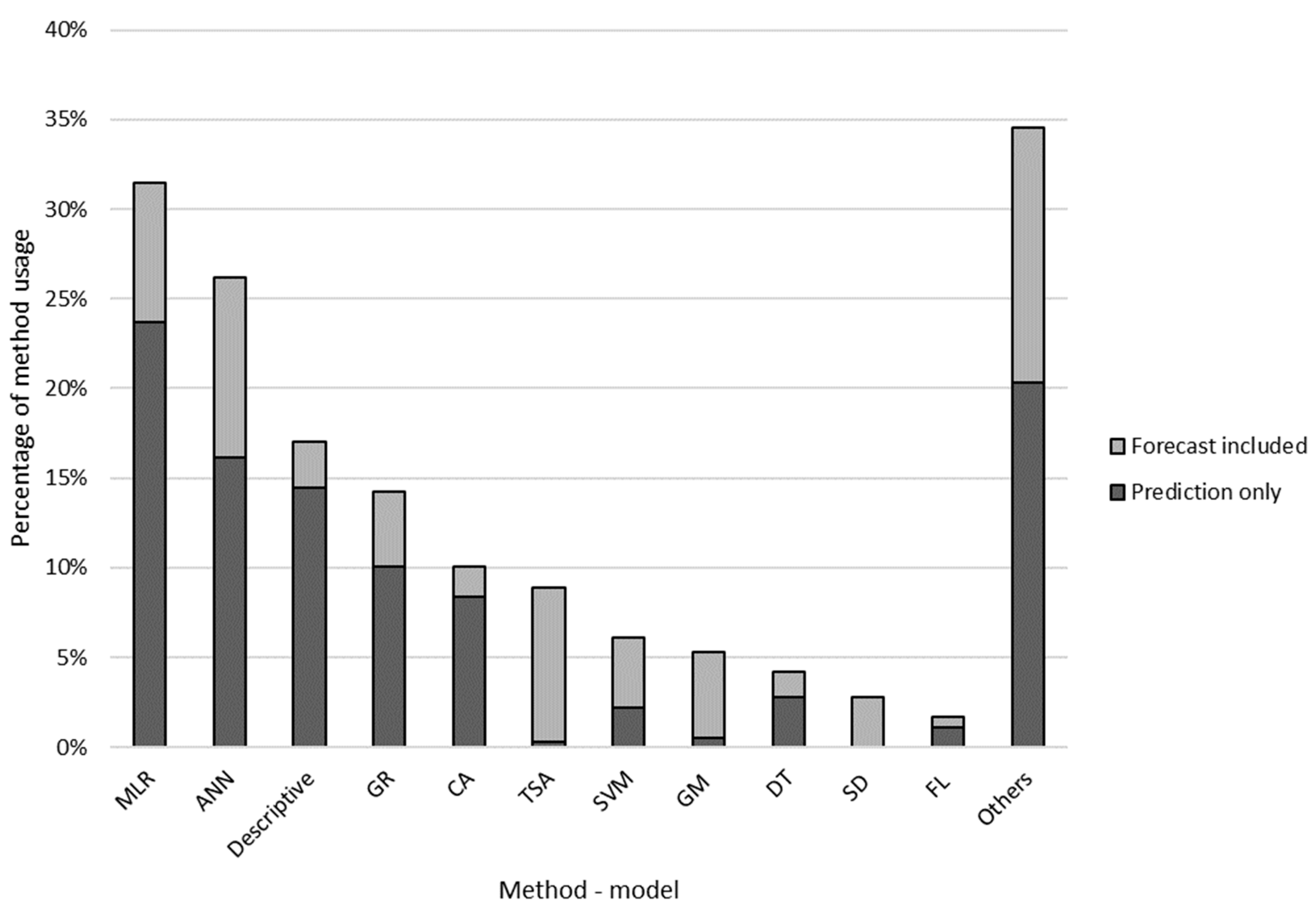
• Utilized methods (columns AU–BF): LR, general regression (GR), TSA, ANN, etc.
• Processing (columns BG–BH): pre-processing (yes/no), verification of assumptions for LR.
• Model quality (columns BI–BM): coefficient of determination (R²), mean absolute error (MAE), mean absolute percentage error (MAPE), etc.

2.1.1. Data Pre-Processing

Pre-processing is included in 26% of the papers, but it is often introduced very briefly without a detailed description of the actual procedures used. Only 60 papers out of 359 involved pre-processing and simultaneously evaluated the quality of the developed model. Approximately 32% of these 60 articles with pre-processing used weekly or daily data [24] and about 47% of the articles with pre-processing used annual data. However, the models with annual data are usually created on many territorial units, where, again, it was possible to use common methods such as z-score [25], Grubb’s test, or Dixon’s test [26]. Outliers occurring in a short time series were often dealt with expertly. The authors’ recommendations regarding the pre-processing of short time series are provided in Section 4.2. It should be mentioned that pre-processing did not address changepoint detection in the studied papers, although it can have a major impact on the model.

2.1.2. The Detail of a Dataset

The selected publications focused on different waste types, as shown in Figure 1. The most frequently modeled component was MSW, at 54%. This was followed by the separately collected waste with high potential for material recovery (paper, plastics, glass, bio-waste), with a frequency of about 15%. Separated waste (SEP) was also modeled as one stream, i.e., the separately collected but not individually distinguished components of MSW. It is worth noting that a relatively small percentage of the publications (6%) focused on MMW generation (terminology is not uniform, in some publications also called residual waste). The reason for this might have been that this stream is quite difficult to model due to the relationship between MMW and the sorted components.

The following territorial divisions were monitored: state, region, municipality, household, building, hospital and “others” (which included all the remaining levels due to their infrequent occurrence). Some territorial divisions were directly related to specific waste types, e.g., building (construction and demolition waste), hospital, hotel, or aircraft. Figure 2 shows the relationship of the territorial detail with the time division and the input data acquisition method. The household data were most often available on a daily basis (more than 55%). This was because they came from surveys in which the produced waste was commonly collected from a sample of households and weighed every day. The national-level data, on the other hand, were available yearly in 87% of cases.

Regarding the household-level data (waste generation and socio-economic information), they were usually obtained via surveys or interviews. Existing databases about reports were mostly used as the source for collecting the data for hierarchically higher levels (municipality, region, state).

2.1.3. Approaches Applied

The values in Figure 3 indicate the shares of papers utilizing each method (please note that some articles employed multiple methods). The most common method—appearing in 31% of the studies—was MLR. In this case, the waste generation was estimated based on the available sociological, economic, demographic, and other data. ANN, which belongs to artificial intelligence methods and has become increasingly popular in recent years, was the second most used (26% approach), followed by the simple descriptive approach and general regression—GR (e.g., generalized linear model—GLM, analysis of variance—ANOVA, or nonlinear regression). Some publications also featured other methods than those listed explicitly in Figure 3 (grouped under “Others”). These included, for instance, mass balance, the theory of planned behavior, or models based on geographical information systems (GIS). The colors in the respective composite bar chart indicate whether the models described in the evaluated papers were predictive or included forecasting as well.

Several models were tested in paper [27], of which the most accurate results were obtained for the utilized data set using gamma regression (GLM). Karpušenkaitė et al. (2016) [28] tested different models for a specific waste fraction (namely, medical waste), and different time series lengths. The result was that no universally applicable model exists, but the GLM models provided the best results for the regional-level data. Kannangara et al. (2018) [29] compared DT and ANN and found that ANN achieved higher accuracy, while the results from DT could be interpreted more clearly. According to [23], 45% of WM papers using ANN worked with at most 100 data points, but ANN have still become popular in WM. Petridis et al. (2016) [30] compared different models for time series, and autoregressive moving average (ARMA) provided the most accurate results, but the Box-Jenkinson methodology (ARMA, autoregressive integrated moving average—ARIMA, and their modifications) achieves good results on long time series. Ghinea et al. (2016) [5] presented S-curve models as the most suitable option for trend analyses depending on the data available.

A different route is followed by hybrid models, which combine the advantages of the individual methods used. Xu et al. (2013) [31] showed that the combination of the seasonal ARIMA (SARIMA) and grey system was robust enough to fit the seasonal and annual dynamic behavior of waste generation. However, the mentioned models are focused on the specific waste fraction, and general applicability cannot be deduced. This is a feature of most of the models in the review. The methodology proposed in [32] combined the S-curve trend and ANN, where for the future construction projects, the S-curve trend was linked to the project characteristics via the ANN forecasting of waste generation. Trend analysis, followed by correcting the estimates to maintain the hierarchical links in the system, was supplemented by data reconciliation in the methodology presented in [33].

The selection of the suitable methods depends mainly on the nature of the input data and the objectives of the model. The evaluation of the model quality presented in various studies is problematic because of the different input data qualities, verification of compliance with method assumptions, or model refitting risk. However, generally, it holds true that higher-quality models can be obtained at higher levels of territorial division due to lower data variability.

2.2. Evaluation of Review

The review showed the possibilities of using different modeling methods, and a summary of the main outputs is shown in Figure 4. The numerical value indicates how many models, out of a total of 359 publications, correspond to the given characteristic. It should be noted that one publication may include several types of models, e.g., for testing reasons or when using a hybrid method. Therefore, the sum of the values in one layer does not have to correspond to the value in a higher layer. Attention is paid to the forecasting models (130 publications out of 359); the prediction models for current waste generation were previously addressed in the publication [15]. Forecasting models can be divided into two basic types. One of them only works with historical data on waste generation and models the development over time. These models use common approaches of TSA. The eventual principles of ANN, GR, MLR, etc. are applied for modeling the trend in the data, where time is the only independent variable. The second type models the links between waste generation and various factors (economic, environmental, sociological, etc.). Based on the expected development of these factors, a waste generation forecast is created. This area includes both conventional and machine learning approaches.

The detail of the time division is crucial because it often determines the length of the time series: the annual data create short time series and higher detail can create long time series. The detail of the time series for both types of method (development in the time and links in the system) was divided into year detail and others in Figure 4. The time division is 28/23 (year/others) models for the methods using development in time series and 64/15 (year/others) models for the methods using links in the system. Thus, a total of 92 models use data in the year detail and only 28 models of 92 use methods based on the development in the time. The fundamental problem of methods that use links in the system is the need to forecast all of the influential factors. Usually, forecasts of these factors are not available in the necessary quality and sufficient forecasting length, see [34]. The authors consider it more appropriate to use methods based on time development due to the smaller requirements for input data.

Furthermore, it is desirable to deal with the issue of territorial hierarchy. In most cases, the model is created for one level of territory (state, municipality, etc.). For WM planning, the waste generation forecasts are necessarily for different territorial divisions, but these forecasts are performed separately without the hierarchical links. The review includes only six models that consider the territorial hierarchy for short time series forecasts, and all of these models were previously presented by the authors of this review. Most authors do not consider territorial links (22 models for short time series), which the authors consider as a one of the research gaps.

• The choice of modeling method (Section 3 and Section 4).

The presented studies apply different methods without explaining why a particular method was chosen. Based on the findings, this text provides support for decision-making when choosing a suitable method. Data availability and data properties are primarily taken into account (Section 3). The schematic representation of the suggested decision process is described in Figure 5. In Section 4. the problems found in the modeling and recommendations for their solution are formulated, which should make it easier for the reader to apply the methods further.

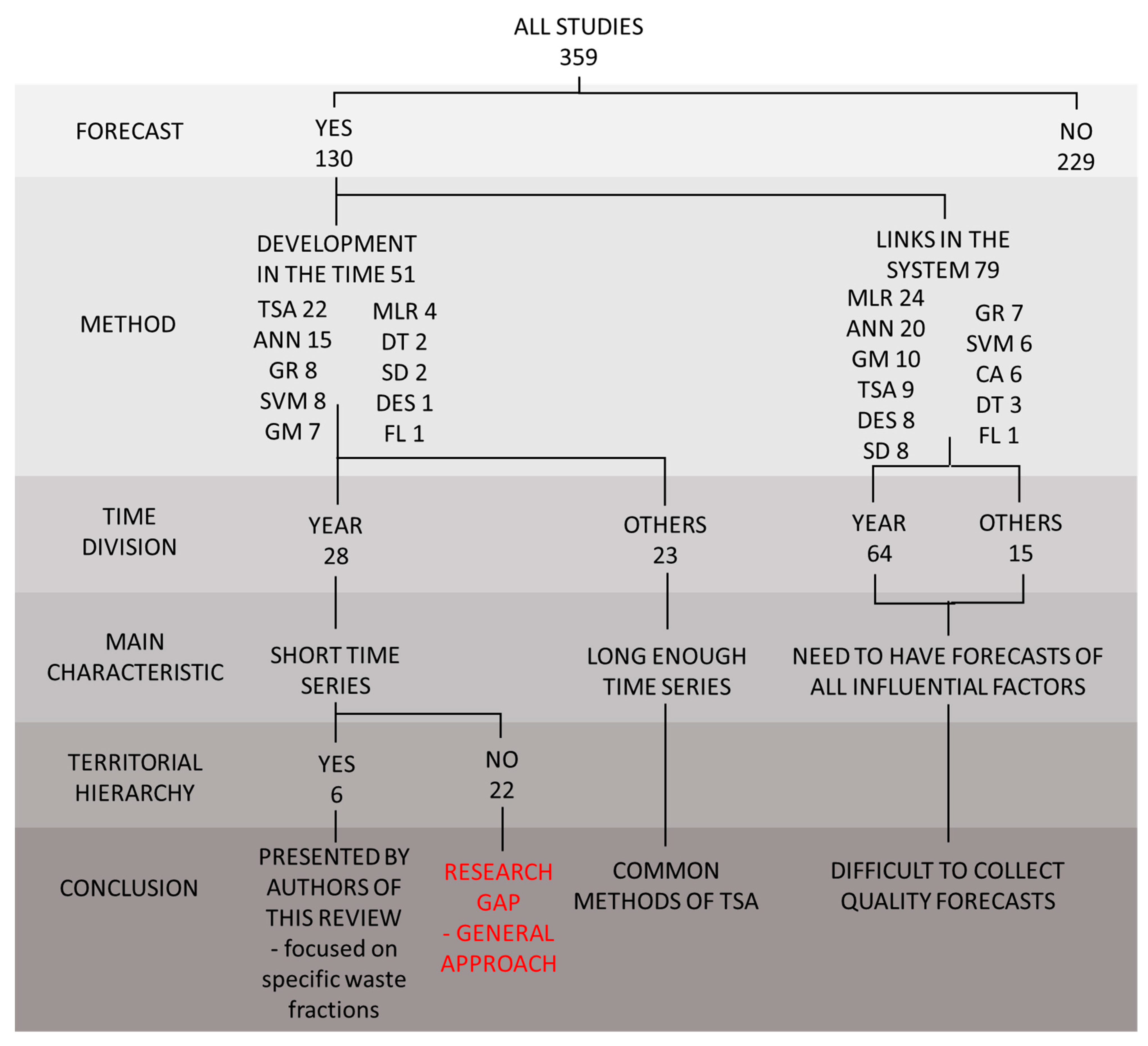
• The general approach of waste generation forecasting (Section 5)

The models mentioned in the literature review (Section 2) are focused on specific waste fractions, and general applicability cannot usually be deduced. This is a feature of most models in the review. Within this manuscript, the approach usable for arbitrary waste fraction is presented (Section 5). The main characteristic of the approach is in the interconnectedness of the forecast and projection, which can achieve the results taking into account real conditions.

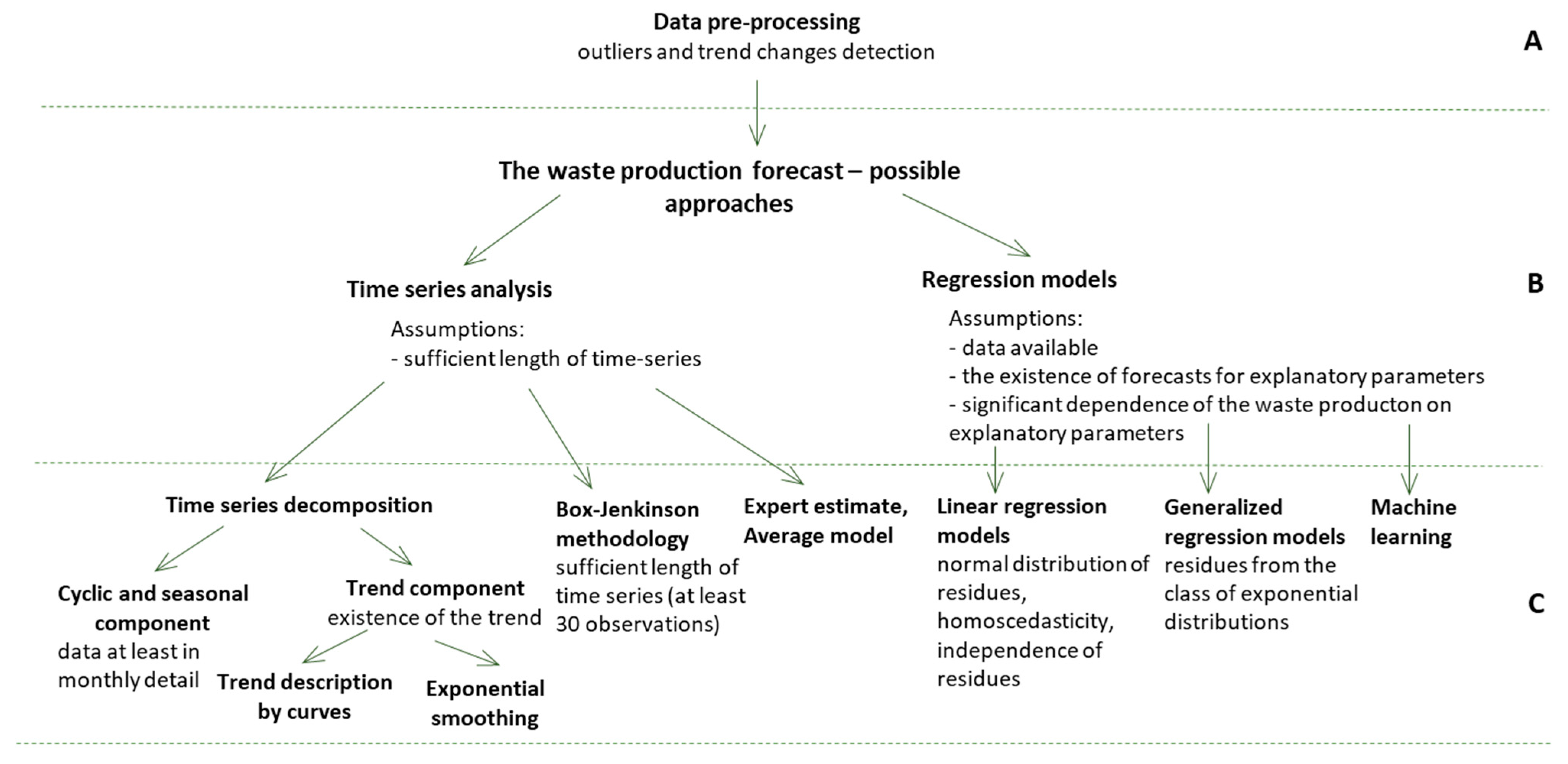
3. The Decision Process for Method Selection

The selection of a suitable modeling method depends on the target application and available data. For the applications presented in Section 1.1, it is advisable to use the models from

Table 2. Representative model types for individual applications.

Application	Most Common Features	Model	Reference
Waste management legislation and policy	- long-term forecasting - smaller data frequency (e.g., years) - larger territorial units (e.g., state)	MLR	[35,36,37]
		ANN	[38,39]
		TSA	[40,41]
		Scenario models	[7,42,43]
Strategic decision-making on waste management infrastructure	- long-term forecasting - smaller data frequency (e.g., years) - different territorial levels (city, region, state)	MLR	[6,44,45]
		DT	[46]
		ANN	[29,47,48]
		TSA	[5,49]
		Scenario models	[50,51]
Operational decision-making in waste management	- shorter-term forecasting - greater data frequency (e.g., months, days) - smaller territorial units (e.g., municipalities)	MLR	[49,52]
		ANN	[53,54]
		TSA	[55,56]
		Scenario models	[57]

. This table shows only the forecasting and projection models, which are necessary for planning the future directions to be taken in WM. For WM legislation and policy tasks (Section 1.1.1), long-term forecasts with less territorial and temporal detail will be more advantageous. The opposite is true in the case of operational decision-making in waste management (Section 1.1.3); that is, short-term forecasting, which will usually require more detail in terms of territory and time, will be most appropriate for this task. If dynamic planning is required, then it is necessary to also take into account the computational complexity of the methods.

Among almost 360 evaluated studies, no GLM model was found to be applied to forecasting. In the case of methods describing waste generation via the influencing factors (MLR, GLM, DT, ANN), it is necessary to forecast all of the influencing factors in advance. This significantly limits the usability of the mentioned methods because forecasts of influencing factors are unavailable or of poor quality. As for TSA, these are mainly trend models for long-term planning. Short-term time series information, such as seasonal effects and autoregression, are essential for operational decision-making.

A general guide to selecting an appropriate forecasting method is shown in Figure 5. The choice of a specific method depends primarily on the number and character of the input data. The flow chart also contains the assumptions and requirements put on the input data. The main steps in the process of forecasting are summarized below:

• I. Conversion of data to unit quantity (with respect to activity rate) and data transformation

Requirement: Activity rate is a significant parameter. Typically, generation per capita is considered to be a unit quantity for MSW. Then, the number of inhabitants represents the activity rate. If desired, the data can be transformed at this stage.

2.

II. Data pre-processing (level A in Figure 5)

Detection of outliers and changes in the trend.

3.

III. Assessment of significant parameters

Requirement: Data for all territorial units of the system.

4.

IV. Selection of the modeling method (level B in Figure 5)

Requirement: Validity of assumptions with respect to the selected method. Sufficient time series length for TSA depends on the method used in level C. Generally, the most stringent limitations are set for cyclic and seasonal components and the Box Jenkinson methodology. Expert estimates and average models, on the other hand, can be applied to only a few data points.

5.

V. Forecasting via the selected method (level C in Figure 5)

Requirement: Validity of assumptions for the respective method.

Figure 5. Forecasting method selection procedure.

Figure 5. Forecasting method selection procedure.

The final forecast should meet the following criteria:

• Compliance with balances and interactions: balance of estimates on different hierarchy levels. The hierarchical structure of territorial units and waste fractions should be maintained [33], see Section 4.3.3.
• Confidence intervals: the expected uncertainty is integral to the results [58]. In most cases, however, information on model uncertainty is missing.
• Evaluation of the model quality: most models involve at least some quality assessment. Several commonly used criteria are R², MAPE, and prediction errors. It is also recommended to verify the quality of the forecast based on the testing data. Before the forecast is made, a certain part of the data at the end of the time series is allocated for this purpose, and then the prediction provided by the model is compared to this pre-allocated data set.

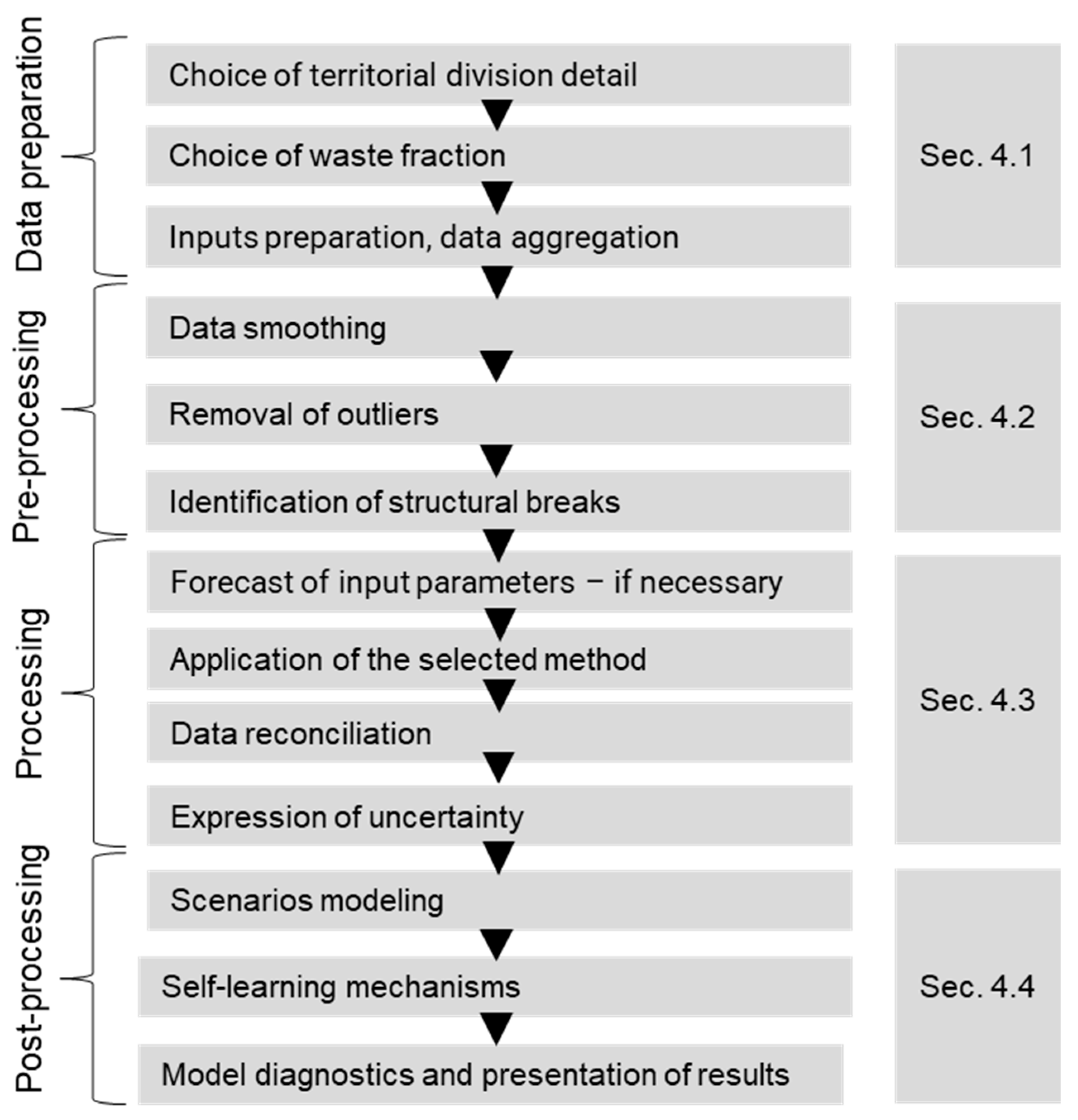
4. Problems and Recommendations for Waste Generation Forecasting

A wide range of theoretical bases for forecasting approaches is provided by [59], but without a link to specific applications in WM. The requirements and processes that are inherent to each waste generation estimate are explained below. Based on the studied publications, the authors of this review proposed a 13-step approach for forecasting, which can be divided into four parts: data preparation, pre-processing, processing, and post-processing. Predictive models are described in detail in the previous papers and will therefore not receive much attention. It is possible to be inspired by predictive models when processing data for forecasting. The following text will formulate the problems (P) and recommendations (R) for the individual forecasting steps based on the experience of the authors and the comprehensive review of the published papers. Almost every article dealing with waste-related data features some steps from Figure 6 and, therefore, potential research gaps will also be specified for issues that have not been sufficiently addressed.

4.1. Data Preparation

P1: The use of historical data within time series can be complicated due to a change in the methodology of monitoring and recording this data.

R1: Historical data must be collected using the same methodology. If the methodology changes, it is necessary to delete the data prior to the alteration or to modify the data accordingly. An example is the merging of some waste streams for recording. Then, it is possible to also merge these waste streams in the historical data before the change.

P2: The required data are not available for all variables or territorial units.

R2: The data can be aggregated to obtain the missing values for higher territorial units. Aggregation also reduces data variability, which is more pronounced at lower levels. In addition, the missing data can be added using predictive models (see Section 1.2 [15]).

P3: It is difficult to compare regions in absolute terms due to the different sizes of producers. The analysis is therefore problematic because of extreme values.

R3: The data often needs to be normalized to check the relationships between variables [15]. Normalization or standardization applies to both waste and socio-economic data. The most common is normalization per capita, household or area. The normalization can also be shifted to improve the interpretability (e.g., the number of stores per 1000 inhabitants). If the data are not normalized per capita, it is recommended to discard extreme values in predictive models. Such data usually originate in the capital or other big cities that, due to their size, can have a considerable impact on the model behavior.

P4: Heteroskedasticity frequently occurs in the data.

R4: For some variables, it is recommended to transform the data to obtain a more even distribution of values. Logarithmic transformation is used most often. The logarithm with base 2 is recommended due to the character of the data in WM. However, here, the possible zero values must be treated appropriately. For zero values, the logarithmic transformation is not defined at all, values close to zero will have a disproportionately significant impact in subsequent analyses. At present, the authors do not know a suitable approach for the processing of zero values in logarithmic transformation.

P5: The data on waste generation include waste fractions, which influence the generation of other fractions.

R5: Interdependent waste fractions should be modeled together. For instance, there is a significant interdependence between MMW and SEP [60]. It may be advantageous to forecast the generation of these waste fractions as an aggregate in the absolute value (e.g., MMW + SEP) and, simultaneously, individual fractions as a rate of the total quantity (e.g., MMW/(MMW + SEP)). This will cause smoothing in the data.

4.2. Data Pre-Processing

P1: Historical WM data may be influenced by unknown or complicated regressors (economic cycles).

R1: It is possible to adjust the data for changes in the given parameters over time, such as economic cycles, or one-off situations, such as the COVID-19 pandemic. The adjusted (smoothed) data can then be used for modeling and forecasting.

P2: The presence of outliers negatively impacts the model.

R2: For long time series, it is possible to follow the common methods for the detection of outliers (see, e.g., [24]). These methods, however, are problematic when it comes to short time series (typically annual data) because the methods’ assumptions cannot be confirmed. Therefore, it is necessary to use a combination of approaches and supplement them with an expert view. The authors can recommend the Holt method (for trend cleaning) together with the Grubbs’ test for the identification of outliers in residues.

P3: The common methods for changepoint detection are not suitable due to their short time series [24].

R3: The following points are recommended for changepoint detection:

• Historical data should be standardized. This makes it possible to specify the same critical limit for each time series.
• Use data visualization if the amount of time series allows.
• Do not identify multiple changepoints in one time series if it is not long enough.
• Focus on the angles between the partial subsequences of the time series and the angles of the historical data lines with the x-axis.
• For further calculations, use the part of the time series behind the changepoint.

P4: It is difficult to detect data anomalies (outliers, changepoints) at the endpoints of the time series.

R4: It is risky to mark an anomaly endpoint as an outlier or a changepoint because no subsequent development in the data is known. It is recommended to test the model with and without the endpoint and compare the output ranges. This will verify the effect of the endpoint on the resulting model. The final decision in the consideration of the. removal of the endpoint due to an anomaly is up to the user.

P5: A time series behaves differently than the other time series (i.e., the whole time series has an extreme generation of waste compared to other producers).

R5: If the entire time series features anomalies, it is advisable to look for influencing factors that may affect it. Another option is to test for a possible correlation between neighboring territorial units because the WM characters may be similar in nearby localities. Expert judgment is the only way to assess the results and evaluate the pre-processing quality.

4.3. Data Processing

4.3.1. Forecasting of Input Parameters

P1: Finding models that describe the waste generation based on the input parameters with sufficient accuracy is not guaranteed.

R1: Clustering can be applied to territories, and then the model can be built at the cluster level [61]. By compiling a model for each cluster separately, higher accuracy can be achieved due to local conditions. The different links can be described in specific clusters of territories and increase the model accuracy.

P2: Forecasting models require the forecasts of all their input parameters for the desired level of territorial division [62], but for some influencing factors, these are not available. Alternatively, only short-term forecasts of the influencing factors are available, but they do not cover the entire waste generation forecasting horizon [34]. Enormous uncertainty would enter waste modeling right at the beginning (not to mention the fact that it is not desirable to proceed with flawed input data).

R2: The inclusion of the influencing factors in the waste generation forecast is not suitable if the forecast of the influencing factors does not cover the whole forecasting horizon or there is significant uncertainty. Then, it is recommended to use the principles of TSA. Forecasts of demographic influencing factors differ from other socio-economic characteristics, and it is recommended to include demographic development in WM forecasts [34]. Long-term demographic projections are usually of sufficient accuracy, but unfortunately, they may not be available for smaller regions. It must be noted that demographic models are, in fact, projections because they are created in the form of scenarios [63].

4.3.2. Application of the Selected Method

P1: A specific method for TSA must be chosen concerning the data frequency detail and the length of the time series.

R1: If daily, weekly, or at most monthly data are available, then it is possible to monitor the cyclic and seasonal components, and short-term forecasting usually is possible [49]. Otherwise, when only yearly data are available for aggregated territories (region, state, i.e., most data sets commonly provided by states or government strategic planning agencies), solely the trend can be examined by the regression function [5]. In some cases, it can be advantageous to use Poisson regression. In the comparison with the trend in the form of a nonlinear function, the Poisson regression has less accurate results. However, the advantage is lower computational time.

P2: The choice of the regression function for describing the trend in the data is not clear (several different functions can give similar results).

R2: It is advisable to look for a compromise between the quality of the fitting according to the chosen criteria (e.g., R², MAPE) and the properties of the selected functions. The authors evaluated the following properties as substantial:

• Monotony—the trend over the forecasting horizon should not change from rising to declining and vice versa, so the trend is assumed to be monotonous. Oscillations around the trend caused by the seasonal or cyclical component are not possible to describe in short time series. Requiring monotony will also reduce the risk of model overfitting. It is recommended to use the power function for trend modeling. The advantage is its wide application for both rising and declining trends [34].
• Limited growth—some time series have a very significant growth in historical data (resp. decline), which may be exponential. Such a trend is usual after the system change, e.g., by collecting a new waste fraction. It cannot be expected to continue this trend over the entire forecast horizon. The more likely development is that the waste generation will slow down the growth. In such cases, it is appropriate to model the trend using an S-shaped curve [34].

It is recommended to model the trend with a simple model and a constant value in the following cases, see [34]:

• By excluding data after pre-processing, the time series remains too short for trend estimation. The minimum number of data can be adjusted to the specific length of the time series.
• The trend model in the data using the functions described above is of poor quality. As a criterion recommends using R2, the critical limit R2 can be customized.
• A simple model with a constant value leads to results that are comparable to a more complex model.
• As a special case, time series containing zero generation of waste in recent years should be extrapolated as a zero value–it is not expected to start generating this waste again.

P3: Attention should be paid to possible special cases of the waste streams. For example, the legislation may change, which may then cause a changepoint, etc. Completely new waste streams may also be introduced after the legislative intervention. Historical data then cannot be used for forecasting in the usual manner.

R3: The mentioned special cases should be detected in pre-processing if the change has already been reflected in the historical data. It is possible to consider the trend forecasting even if not all regions have already responded to the change. In other words, more advanced regions may outline the future directions for the less developed ones (Smejkalová et al., 2020 [64]). An analogous idea can be applied at the state level considering countries with differently advanced WM. Other notable special cases represent waste fractions whose quantities are directly influenced by the developments of specific external factors. A typical example is metal waste, which is linked to the purchase price of raw materials. The purchase price is difficult to forecast due to its cyclic behavior, leading to complicated forecasting of the metal waste fraction.

4.3.3. Data Reconciliation

P1: Historical waste generation data can contain internal consistency links, which form a hierarchical structure: the state comprises the regions, the regions comprise the municipalities. These links are not always maintained after applying the selected method (Section 4.3.2).

R1: The authors recommend correcting waste generation models to restore the system links using, for example, a data reconciliation model [33]. It is assumed that the amount of waste generated at a higher territorial unit is equal to the sum of the amounts in the territories that belong to it (e.g., municipalities located in a particular region). The second type of internal balance assumes links between the waste fractions. An example is the effect of separated waste generation on the amount of MMW [10].

P2: The data reconciliation model is significantly affected by the model weight settings, for example, different importance of the results that are balanced.

R2: It is necessary to pay attention to appropriately chosen weights when balancing; weights should be considered both in terms of total waste generation (preferably in the square root) and in terms of the quality of the estimate. In the case of the balance, percentage changes must also be taken into account [34].

P3: An increase in the generation of one fraction does not mean a decrease in the production of another fraction by exactly this amount; that is, the overflow of waste amounts is not consistent.

R3: The interdependence of waste fractions must be captured in a form that corresponds to reality; the values of the transition between the fractions do not have to be equal; individual waste streams are created and disappear [60].

P4: The possibilities of the chosen solver can significantly affect the success of the calculation when the model is stated as a mathematical programming problem.

R4: The data reconciliation model can be formulated in additive or multiplicative form [34]. The multiplicative form has a significant advantage for wastes with high variability between individual fractions. Producers with significantly different waste generations can occur at different levels of the territory. The additive formulation causes numerical and rounding errors. The setting of the model weights also depends on the formulation. In addition, the multiplicative form works with the percentage change, which is a problem in the case of zero values [34].

P5: The solver is not able to find the optimal solution due to the task size or computational complexity problems.

R5: Usually, at least a relaxed solution is available, i.e., the balances are not met exactly. This may not be a problem for some forecasts. In other cases, it is recommended to reduce the optimization task so that smaller sets of waste streams will be balanced, e.g., only for individual catalogue numbers.

4.3.4. Expression of Uncertainty

P1: Each forecast should provide confidence intervals [65], ideally also prediction intervals. If data reconciliation has been carried out (previous step, Section 4.3.3), it is not possible to use common interval constructs with a normal probability distribution around the model mean value.

R1: The authors suggest simulating the confidence and prediction intervals with the bootstrap method. It is possible to use historical data as one of the possible realizations, and then its variance to generate new data sets. A forecast is made for these generated data, which creates different realizations of the forecast. Based on the properties of forecasts for individual realizations, confidence and prediction intervals are compiled [34]. In the case of a limited number of possible generations within the bootstrap, the variance of forecasts for the construction interval is estimated. In this case, approximately 30 bootstraps are considered sufficient [34].

4.4. Data Post-Processing

4.4.1. Modeling of Scenarios

P1: A forecast does not include possible changes to the system, as described in Section 1.2. Projections deviate from a basic forecast because they must obey the model constraints and predefined boundary conditions. It is essential to ensure the feasibility and consistency of a projection.

R1: Legislative interventions take place at the state level or the levels of other self-governing units. The distribution of the projection changes to the micro-region is essential for determining the potential for future development. For analyses associated with the potential to increase the separation of MSW, it is necessary to have available (or at least estimate) the MMW composition, which allows estimating the potential for change. When using projections, it is recommended to consider the links between waste streams [60]. For the projections, it is necessary to determine the potential for change. The following applies to scenario solutions:

• The scenario does not exceed the potential for change which was set for a specific territorial unit.
• All territorial units show a shift towards meeting the scenario if the potential allows it.
• The individual territories do not overtake in terms of the fulfillment of potential and are monotonous.

4.4.2. Self-Learning Mechanisms

P1: The results must be updated when the input data set changes. The change may occur due to the data editing in the original database or the addition of new data on waste generation from the next period.

R1: During model re-evaluation, one must carry out all the forecasting steps specified in Figure 6. When the data are dynamic in nature, it is necessary to react quickly and develop an adequate methodology [66]. As an example, one might mention forecasting utilizing smart technologies such as weight or fill level sensor-equipped containers.

4.4.3. Model Diagnostics and Presentation of Results

P1: The quality of the models must be verified.

R1: The quality of a forecast should be tested using a pre-allocated test data set. In other words, the forecast should be made using a smaller data set, and the results should then be compared with the remaining values that were not used as the model input data. Model verification can also be conducted via confidence intervals.

R2: Forecasts provided by the models must be presented clearly so that their end-users (the decision-makers) can easily interpret them. Methods for representing results visualization can be found in the paper [45]. Another promising approach for communicating the results and incorporating them into the simulation calculations is the gamification approach [67]. Tools based on gamification for strategic planning in waste management provide interactive feedback with respect to the set criteria [68].

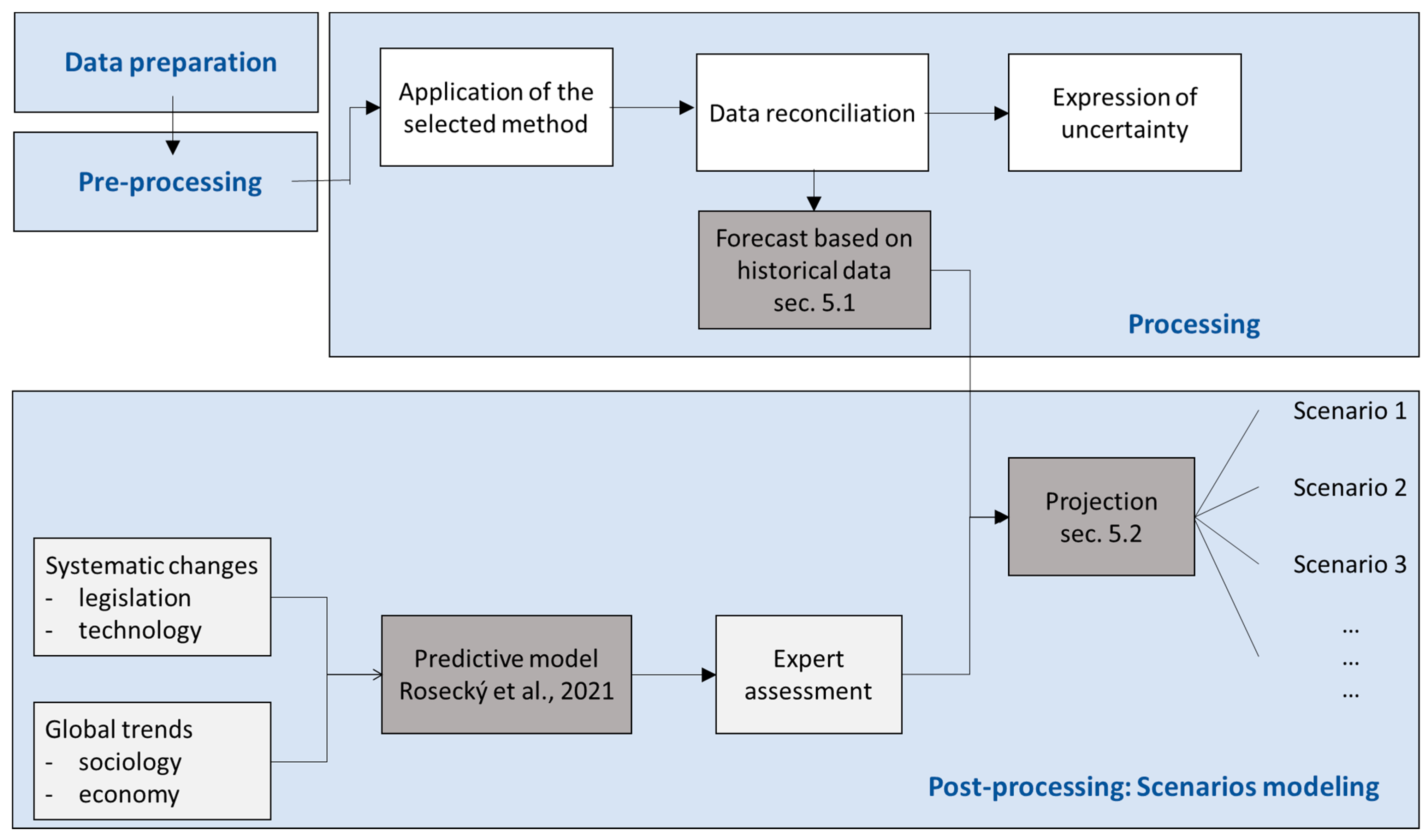
5. Modeling Future Waste Generation and Treatment Based on Short Time Series

Authors of this contribution recommend applying a combination forecast model and a subsequent projection model, see Figure 7. Compared to Figure 6, Figure 7 shows the essential steps of the projection in greater detail. In the first step, a forecast should be created based on historical data, which considers maintaining the current form of WM into the future, see Section 5.1. This part corresponds to data preparation, pre-processing and processing in Figure 6. This is basic information, but waste generation will be affected by systematic changes (legislative, technological etc.) and global trends (sociology, economy etc.) in the real world. Using predictive models, the influence of these factors on waste generation can be estimated, but their development cannot be well forecasted. The expected development of the influencing factors is a matter of expert assessment. Waste generation projection should be a combination of the forecast results with a predictive model, and the impact of the external interventions can be modelled as different scenarios. In the form of scenarios, an estimate of future waste generation can be achieved, which will correspond as best as possible to the real conditions.

5.1. Waste Generation and Treatment Forecast

It is recommended to apply a method based on trend analysis with subsequent data reconciliation in order to maintain hierarchical links in the data [34]. The trend in the historical data can be modelled by the suitable curve. The model of the waste generation trend $p_t$ is significantly affected by the type of the curve $f_t$ (1), where t is the index of time including both the historical data and a forecast.

$$p_t=f_t.$$

(1)

Designation $f_t$ indicates the curve that is recommended in the form of power function (2) or logistic function (3) based on the data character:

$$p_t=a+b{t}^c,$$

(2)

$$p_t=\frac{1}{1+e^{-\left(a+bt\right)}}.$$

(3)

where $a$, $b$, $c$ are the regression coefficients. A model that fits the historical data well is extrapolated to cover the entire forecasting horizon.

The trend estimates do not generally maintain the hierarchical links, i.e., the sum of the regional trends does not correspond to the national trend and similarly for other links. Therefore, it is recommended to apply data reconciliation to ensure these links. This is achieved by a set of constraints. For the territorial hierarchy, this is constraint (4), where $A_{j,\overline{j}}$ defines the relations between territories ($j$ is a superior territorial unit and $\overline{j}$ is a lower territory).

$$k_j={\displaystyle \sum }_{\overline{j}\in J}{A}_{j,\overline{j}}{k}_{\overline{j}}.\hspace{1em}\hspace{1em}\hspace{1em}\hspace{1em}\hspace{1em}\forall j\in J.$$

(4)

Constraints in the case of links between waste fractions can also be formulated similarly. Equation (5) connects the waste generation input data $p_j$ in particular time with the model variable $k_j$ and the waste generation data error ${\epsilon }_j$ in the form of additive notation. In some cases, for reasons of solvability, the multiplicative form of notation is more advantageous.

$$k_j=p_j+{\epsilon }_j.\hspace{1em}\hspace{1em}\hspace{1em}\hspace{1em}\hspace{1em}\forall j\in J,$$

(5)

Equation (6) represents the objective function for the variant with weights $v_j$ to take into account the size of the producer and weights $w_j$ according to quality of fitting.

$${\displaystyle \sum }_{j\in J}{\left(v_j{w}_j\right)}^2\left[{\left({\epsilon }_j^{+}\right)}^2+{\left({\epsilon }_j^{-}\right)}^2\right].$$

(6)

The result of the performed data reconciliation is a forecast based on historical data; this is a basic scenario, further marked BAU (business-as-usual scenario).

5.2. Waste Generation and Treatment Projection

Projections of waste generation are usually formed to meet some targets that are set for aggregated territory (national level). The default information is forecast (BAU, Section 5.1), which is modified to achieve the conditions formulated in the scenario. It is assumed that interventions can influence waste separation and waste generation prevention. The increase in the waste separation within the scenario is caused by the higher separation of the modelled fraction $f$ (e.g., paper, plastics, glass) from unseparated waste u (e.g., MMW, bulky waste). Thus, the expert assessment includes setting the following parameters:

• percentage waste prevention ($pre{v}^{SC,N1}$: $SC$—marking the scenario, $N1$—territorial level NUTS1),
• separation rate of individual assessed waste fractions ($S{R}_{u,f}^{SC,N1}$: $u$—unseparated waste fraction, $f$—modelled waste fraction).

The main results of scenario $SC$ on aggregated territory $N1$ are:

• Separated waste $k_{u,f}^{SC,N1}$.

The generation of separated waste $f$, which originates in the unseparated fraction $u$, is determined according to (7). The expression $k_{u,f}^{BAU,N1}+l_{u,f}^{BAU,N1}$ means the total generation of fraction $f$ according to BAU, i.e., separated $k_{u,f}^{BAU,N1}$ originates in u and rest of f in unseparated fraction $l_{u,f}^{BAU,N1}$ amount. From the total generation, the separated amount is determined using the separation rate $S{R}_{u,f}^{SC,N1}$, and the impact of prevention is also taken into account as $\left(1-pre{v}^{SC,N1}\right)$.

• Waste $f$in unseparated waste $u$: $l_{u,f}^{SC,N1}$.

The result of this point is therefore the composition of the unseparated waste u, and it is determined according to Equation (8). The principle is similar to the previous point for separated waste $k_{u,f}^{SC,N1}$, only the supplement to the separation rate is considered as $\left(1-S{R}_{u,f}^{SC,N1}\right)$.

• Total unseparated waste $\left(L_u^{SC,N1}\right)$.

The generation of the unseparated waste u is given by (9). It comes from the generation of u in BAU $\left(L_u^{BAU,N1}\right),$ which is reduced by the prevention in the form $\left(1-pre{v}^{SC,N1}\right)$. The waste that was separated according to the scenario SC is deducted from this amount. The separation of waste f in the scenario SC is determined as the difference between quantity in BAU given by ${\displaystyle \sum }_{f\in F}{l}_{u,f}^{BAU,N1}\left(1-pre{v}^{SC,N1}\right)$ and the new quantity in $SC$ scenario given by ${\displaystyle \sum }_{f\in F}{l}_{u,f}^{SC,N1}$.

$$k_{u,f}^{SC,N1}=\left(1-pre{v}^{SC,N1}\right)\left(k_{u,f}^{BAU,N1}+l_{u,f}^{BAU,N1}\right)S{R}_{u,f}^{SC,N1}\hspace{1em}\hspace{1em}\hspace{1em}\hspace{1em}\hspace{1em}\forall u\in U, \forall f\in F$$

(7)

$$l_{u,f}^{SC,N1}=\left(k_{u,f}^{BAU,N1}+l_{u,f}^{BAU,N1}\right)\left(1-S{R}_{u,f}^{SC,N1}\right)\left(1-pre{v}^{SC,N1}\right)\hspace{1em}\hspace{1em}\hspace{1em}\hspace{1em}\hspace{1em}\forall u\in U, \forall f\in F$$

(8)

$$L_u^{SC,N1}=L_u^{BAU,N1}\left(1-pre{v}^{SC,N1}\right)-\left({\displaystyle \sum }_{f\in F}{l}_{u,f}^{BAU,N1}\left(1-pre{v}^{SC,N1}\right)-{\displaystyle \sum }_{f\in F}{l}_{u,f}^{SC,N1}\right)\hspace{1em}\hspace{1em}\hspace{1em}\hspace{1em}\hspace{1em}\forall u\in U$$

(9)

The result of the SC scenario at the aggregated (national) level, given by (7)–(9), should be subsequently divided into lower territorial units, down to the municipalities, because the national WM is the result of the activities of the lower units (municipalities). It is recommended to divide the scenario for the national level (N1) to the level of municipalities (L2) according to the potential that individual municipalities have for waste separation improvement. A suitable indicator of this potential may be the separation rate.

The goal of the presented approach is a suggestion of a general approach that is applicable to any waste fraction based on short time series. At the same time, it is a unique approach, combining the principles of forecasting with the consideration of influential factors through scenarios. Thanks to modelled scenarios, the expected variability of waste generation is taken into account, which will enable more efficient planning of WM.

6. Conclusions

Over the years, various methods used for waste generation modeling have been proposed. Prediction, forecasting, and projection must be distinguished, while the use of various approaches depends on the specific application in WM. A deficiency was found in that a significant number of past publications have been devoted to designing a suitable modeling method. However, the authors recommend paying attention to the quality of the input data, which has been minimal in the reviewed papers. It is important to remember that input data are essential for every model. In addition, the end-user of a forecast, prediction, or projection must be provided with the model uncertainties in the form of confidence intervals or several scenarios. This is another key part of each model that was missing in the majority of the evaluated papers on WM modeling. Although many methods do not offer a direct way of expressing the model uncertainty, bootstrapping can be used to at least estimate it.

The data set available, its territorial and temporal detail, and the prediction horizon are decisive for the modeling method choice. As prediction models have already been elaborated in greater detail [15], most of the text is devoted to forecasts and projections. The authors formulated the decisive process for the choice of modeling method, which provides unique support for further forecasters. In summary, if the influencing factors and their links to waste generation are used for modeling, the influencing factors must be forecasted as well. The use of TSA is often limited by its requirements of time series length. In addition, the presented methods are intended for specific waste fractions. Based on the mentioned conclusions of the review, the authors presented a general approach for forecasting. To use this method, it is necessary to have a time series of historical data on waste generation. Compared to other TSA-based methods, a significantly shorter time series is sufficient. The calculation of the method is based on the optimization task of nonlinear programming. The user must therefore have software suitable for this calculation with adequate solvers (CONOPT, KNITRO, etc.). The main feature of forecasting is that it models future developments while maintaining historical conditions. The impact of changing the influential factors on waste generation can be implemented in the forecast in the form of scenarios.

References

1. Directive 2008/98/EC of the European Parliament and of the Council of 19 November 2008 on Waste and Repealing Certain Directives (Text with EEA Relevance). Available online: https://eur-lex.europa.eu/legal-content/ES/TXT/PDF/?uri=CELEX:32008L0098&from=EN (accessed on 23 June 2020).
2. Gardiner, R.; Hajek, P. Municipal waste gener ation, R&D intensity, and economic growth nexus—A case of EU regions. Waste Manag. 2020, 114, 124–135. [Google Scholar] [CrossRef]
3. Directive EU 2018/851 of the European Parliament and of the Council of 30 May 2018 amending Directive 2008/98/EC on Waste (Text with EEA Relevance). Available online: https://eur-lex.europa.eu/legal-content/EN/TXT/PDF/?uri=CELEX:32018L0851&rid=5 (accessed on 23 June 2020).
4. Directive EU 2018/850 of the European Parliament and of the Council of 30 May 2018 amending Directive 1999/31/EC on the landfill of waste (Text with EEA relevance). Available online: https://eur-lex.europa.eu/legal-content/EN/TXT/PDF/?uri=CELEX:32018L0850&rid=3 (accessed on 23 June 2020).
5. Ghinea, C.; Drăgoi, E.N.; Comăniţă, E.-D.; Gavrilescu, M.; Câmpean, T.; Curteanu, S.; Gavrilescu, M. Forecasting municipal solid waste generation using prognostic tools and regression analysis. J. Environ. Manag. 2016, 182, 80–93. [Google Scholar] [CrossRef] [PubMed]
6. Ayeleru, O.O.; Okonta, F.N.; Ntuli, F. Municipal solid waste generation and characterization in the City of Johannesburg: A pathway for the implementation of zero waste. Waste Manag. 2018, 79, 87–97. [Google Scholar] [CrossRef]
7. Mena-Nieto, A.; Estay-Ossandon, C.; dos Santos, S.P. Will the Balearics and the Canary Islands meet the European Uniontargets for municipal waste? A comparative study from 2000 to 2035. Sci. Total Environ. 2021, 783, 147081. [Google Scholar] [CrossRef]
8. Tomić, T.; Dominković, D.F.; Pfeifer, A.; Schneider, D.R.; Pedersen, A.S.; Duić, N. Waste to energy plant operation under the influence of market and legislation conditioned changes. Energy 2017, 137, 1119–1129. [Google Scholar] [CrossRef]
9. Ilbahar, E.; Kahraman, C.; Cebi, S. Location selection for waste-to-energy plants by using fuzzy linear programming. Energy 2021, 234, 121189. [Google Scholar] [CrossRef]
10. Pavlas, M.; Šomplák, R.; Smejkalová, V.; Stehlík, P. Municipal Solid Waste Fractions and Their Source Separation: Forecasting for Large Geographical Area and Its Subregions. Waste Biomass Valorization 2020, 11, 725–742. [Google Scholar] [CrossRef]
11. Bramati, C.M. Waste generation and regional growth of marine activities an econometric model. Mar. Pollut. Bull. 2016, 112, 151–165. [Google Scholar] [CrossRef] [PubMed]
12. Ghiani, G.; Laganà, D.; Manni, E.; Triki, C. Capacitated location of collection sites in an urban waste management system. Waste Manag. 2012, 32, 1291–1296. [Google Scholar] [CrossRef] [PubMed]
13. Nie, X.H.; Huang, G.H.; Li, Y.P.; Liu, L. IFRP: A hybrid interval-parameter fuzzy robust programming approach for waste management planning under uncertainty. J. Environ. Manag. 2007, 84, 1–11. [Google Scholar] [CrossRef]
14. Koç, C.; Bektaş, T.; Jabali, O.; Laporte, G. Thirty years of heterogeneous vehicle routing. Eur. J. Oper. Res. 2016, 249, 1–21. [Google Scholar] [CrossRef]
15. Rosecký, M.; Šomplák, R.; Slavík, J.; Kalina, J.; Bulková, G.; Bednář, J. Predictive modelling as a tool for effective municipal waste management policy at different territorial levels. J. Environ. Manag. 2021, 291, 112584. [Google Scholar] [CrossRef] [PubMed]
16. Beigl, P.; Lebersorger, S.; Salhofer, S. Modelling municipal solid waste generation: A review. Waste Manag. 2008, 28, 200–214. [Google Scholar] [CrossRef] [PubMed]
17. Cherian, J.; Jacob, J. Management models of municipal solid waste: A review focusing on socio economic factors. Int. J. Econ. Financ. 2012, 4, 131–139. [Google Scholar] [CrossRef]
18. Kolekar, K.A.; Hazra, T.; Chakrabarty, S.N. A review on prediction of municipal solid waste generation models. Procedia Environ. Sci. 2016, 35, 238–244. [Google Scholar] [CrossRef]
19. Goel, S.; Ranjan, V.P.; Bardhan, B.; Hazra, T. Forecasting solid waste generation rates. Modelling Trends in Solid and Hazardous. Waste Manag. 2017, 20, 35–64. [Google Scholar] [CrossRef]
20. Alzamora, B.R.; Barros, R.T.D.V.; de Oliveira, L.K.; Gonçalves, S.S. Forecasting and the influence of socioeconomic factors on municipal solid waste generation: A literature review. Environ. Dev. 2022, 44, 100734. [Google Scholar] [CrossRef]
21. Abdallah, M.; Talib, M.A.; Feroz, S.; Nasir, Q.; Abdalla, H.; Mahfood, B. Artificial intelligence applications in solid waste management: A systematic research review. Waste Manag. 2020, 109, 231–246. [Google Scholar] [CrossRef]
22. Guo, H.-N.; Wu, S.-B.; Tian, Y.-J.; Zhang, J.; Liu, H.-T. Application of machine learning methods for the prediction of organic solid waste treatment and recycling processes: A review. Bioresour. Technol. 2021, 319, 124114. [Google Scholar] [CrossRef]
23. Xu, A.; Chang, H.; Xu, Y.; Li, R.; Li, X.; Zhao, Y. Applying artificial neural networks (ANNs) to solve solid waste-related issues: A critical review. Waste Manag. 2021, 124, 385–402. [Google Scholar] [CrossRef]
24. Blázquez-García, A.; Conde, A.; Mori, U.; Lozano, J.A. A review on outlier/anomaly detection in time series data. arXiv 2020, arXiv:abs/2002.04236. [Google Scholar] [CrossRef]
25. Aggarwal, V.; Gupta, V.; Singh, P.; Sharma, K.; Sharma, N. Detection of spatial outlier by using improved Z-score test. In Proceedings of the International Conference on Trends in Electronics and Informatics, Tirunelveli, India, 23–25 April 2019; pp. 788–790. [Google Scholar] [CrossRef]
26. De Muth, J.E. Tests to Evaluate Potential Outliers. APS Adv. Pharm. Sci. Ser. 2019, 40, 197–210. [Google Scholar] [CrossRef]
27. Ibáñez, M.V.; Prades, M.; Simó, A. Modelling municipal waste separation rates using generalized linear models and beta regression. Resour. Conserv. Recycl. 2011, 55, 1129–1138. [Google Scholar] [CrossRef]
28. Karpušenkaitė, A.; Ruzgas, T.; Denafas, G. Forecasting medical waste generation using short and extra short datasets: Case study of Lithuania. Waste Manag. Res. 2016, 34, 378–387. [Google Scholar] [CrossRef]
29. Kannangara, M.; Dua, T.; Ahmadi, L.; Bensebaa, F. Modeling and prediction of regional municipal solid waste generation and diversion in Canada using machine learning approaches. Waste Manag. 2018, 74, 3–15. [Google Scholar] [CrossRef]
30. Petridis, N.E.; Stiakakis, E.; Petridis, K.; Dey, P. Estimation of computer waste quantities using forecasting techniques. J. Clean. Prod. 2016, 112, 3072–3085. [Google Scholar] [CrossRef]
31. Xu, L.; Gao, P.; Cui, S.; Liu, C. A hybrid procedure for MSW generation forecasting at multiple time scales in Xiamen City, China. Waste Manag. 2013, 33, 1324–1331. [Google Scholar] [CrossRef] [PubMed]
32. Lu, W.; Peng, Y.; Chen, X.; Skitmore, M.; Zhang, X. The S-curve for forecasting waste generation in construction projects. Waste Manag. 2016, 56, 23–34. [Google Scholar] [CrossRef] [PubMed]
33. Pavlas, M.; Šomplák, R.; Smejkalová, V.; Nevrlý, V.; Zavíralová, L.; Kůdela, J.; Popela, P. Spatially distributed generation data for supply chain models—Forecasting with hazardous waste. J. Clean. Prod. 2017, 161, 1317–1328. [Google Scholar] [CrossRef]
34. Smejkalová, V.; Šomplák, R.; Pluskal, J.; Rybová, K. Hierarchical optimisation model for waste management forecasting in EU. Optim. Eng. 2022, 23, 2143–2175. [Google Scholar] [CrossRef]
35. Andersen, F.M.; Larsen, H.V. FRIDA: A model for the generation and handling of solid waste in Denmark. Resour. Conserv. Recycl. 2012, 65, 47–56. [Google Scholar] [CrossRef]
36. Hřebíček, J.; Kalina, J.; Soukopová, J.; Horáková, E.; Prášek, J.; Valta, J. Modelling and forecasting waste generation—DECWASTE information system. IFIP Adv. Inf. Commun. Technol. 2017, 507, 433–445. [Google Scholar] [CrossRef]
37. Awasthi, A.K.; Cucchiella, F.; D’Adamo, I.; Li, J.; Rosa, P.; Terzi, S.; Wei, G.; Zeng, X. Modelling the correlations of e-waste quantity with economic increase. Sci. Total Environ. 2017, 613, 46–53. [Google Scholar] [CrossRef]
38. Chhay, L.; Reyad, M.A.H.; Suy, R.; Islam, M.R.; Mian, M.M. Municipal solid waste generation in China: Influencing factor analysis and multi-model forecasting. J. Mater. Cycles Waste Manag. 2018, 20, 1761–1770. [Google Scholar] [CrossRef]
39. Yusoff, S.H.; Din, U.N.K.A.; Mansor, H.; Midi, N.S.; Zaini, S.A. Neural network prediction for efficient waste management in Malaysia. Indones. J. Electr. Eng. Comput. Sci. 2018, 12, 738–747. [Google Scholar] [CrossRef]
40. Karpušenkaitė, A.; Ruzgas, T.; Denafas, G. Time-series-based hybrid mathematical modelling method adapted to forecast automotive and medical waste generation: Case study of Lithuania. Waste Manag. Res. 2018, 36, 454–462. [Google Scholar] [CrossRef]
41. Islam, M.T.; Huda, N. E-waste in Australia: Generation estimation and untapped material recovery and revenue potential. J. Clean. Prod. 2019, 237, 117787. [Google Scholar] [CrossRef]
42. Cole, C.; Quddus, M.; Wheatley, A.; Osmani, M.; Kay, K. The impact of Local Authorities’ interventions on household waste collection: A case study approach using time series modelling. Waste Manag. 2014, 34, 266–272. [Google Scholar] [CrossRef] [PubMed]
43. Klavenieks, K.; Blumberga, D. Forecast of Waste Generation Dynamics in Latvia. Energy Procedia 2016, 95, 200–207. [Google Scholar] [CrossRef] [Green Version]
44. Lebersorger, S.; Beigl, P. Municipal solid waste generation in municipalities: Quantifying impacts of household structure, commercial waste and domestic fuel. Waste Manag. 2011, 31, 1907–1915. [Google Scholar] [CrossRef] [PubMed]
45. Chen, D.M.-C.; Bodirsky, B.L.; Krueger, T.; Mishra, A.; Popp, A. The world’s growing municipal solid waste: Trends and impacts. Environ. Res. Lett. 2020, 15, 074021. [Google Scholar] [CrossRef]
46. Johnson, N.E.; Ianiuk, O.; Cazap, D.; Liu, L.; Starobin, D.; Dobler, G.; Ghandehari, M. Patterns of waste generation: A gradient boosting model for short-term waste prediction in New York City. Waste Manag. 2017, 62, 3–11. [Google Scholar] [CrossRef] [PubMed]
47. Vu, H.L.; Ng, K.T.W.; Bolingbroke, D. Time-lagged effects of weekly climatic and socio-economic factors on ANN municipal yard waste prediction models. Waste Manag. 2019, 84, 129–140. [Google Scholar] [CrossRef] [PubMed]
48. Sunayana; Kumar, S.; Kumar, R. Forecasting of municipal solid waste generation using nonlinear autoregressive (NAR) neural models. Waste Manag. 2021, 121, 206–214. [Google Scholar] [CrossRef]
49. Denafas, G.; Ruzgas, T.; Martuzevičius, D.; Shmarin, S.; Hoffmann, M.; Mykhaylenko, V.; Ogorodnik, S.; Romanov, M.; Neguliaeva, E.; Chusov, A.; et al. Seasonal variation of municipal solid waste generation and composition in four East European cities. Resour. Conserv. Recycl. 2014, 89, 22–30. [Google Scholar] [CrossRef]
50. Dwivedy, M.; Mittal, R.K. Future trends in computer waste generation in India. Waste Manag. 2010, 30, 2265–2277. [Google Scholar] [CrossRef]
51. Komwit, S.; Chompoonuh, K.P. Effects of area characteristics and municipal waste collection fees on household waste generation. J. Mater. Cycles Waste Manag. 2020, 22, 89–96. [Google Scholar] [CrossRef]
52. Gu, B.; Fujiwara, T.; Jia, R.; Duan, R.; Gu, A. Methodological aspects of modeling household solid waste generation in Japan: Evidence from Okayama and Otsu cities. Waste Manag. Res. 2017, 35, 1237–1246. [Google Scholar] [CrossRef]
53. Yang, Y.; Yuan, G.; Cai, J.; Wei, S. Forecasting of disassembly waste generation under uncertainties using digital twinning-based hidden Markov model. Sustainability 2021, 13, 5391. [Google Scholar] [CrossRef]
54. Song, J.; He, J.; Zhu, M.; Tan, D.; Zhang, Y.; Ye, S.; Shen, D.; Zou, P. Simulated annealing based hybrid forecast for improving daily municipal solid waste generation prediction. Scinetific World J. 2014, 834357. [Google Scholar] [CrossRef]
55. Rimaityté, I.; Ruzgas, T.; Denafas, G. Application and evaluation of forecasting methods for municipal solid waste generation in an eastern-European city. Waste Manag. Res. 2012, 30, 89–98. [Google Scholar] [CrossRef]
56. Montecinos, J.; Ouhimmou, M.; Chauhan, S.; Paquet, M. Forecasting multiple waste collecting sites for the agro-food industry. J. Clean. Prod. 2018, 187, 932–939. [Google Scholar] [CrossRef]
57. Long, F.; Song, B.; Wang, Q.; Xia, X.; Xue, L. Scenarios simulation on municipal plastic waste generation of different functional areas of Beijing. J. Mater. Cycles Waste Manag. 2012, 14, 250–258. [Google Scholar] [CrossRef]
58. Abbasi, M.; Abduli, M.A.; Omidvar, B.; Baghvand, A. Results uncertainty of support vector machine and hybrid of wavelet transform-support vector machine models for solid waste generation forecasting. Environ. Prog. Sustain. Energy 2014, 33, 220–228. [Google Scholar] [CrossRef]
59. Petropoulos, F.; Apiletti, D.; Assimakopoulos, V.; Babai, M.Z.; Barrow, D.K.; Ben Taieb, S.; Bergmeir, C.; Bessa, R.J.; Bijak, J.; Boylan, J.E.; et al. Forecasting: Theory and practice. Int. J. Forecast. 2022, 38, 705–871. [Google Scholar] [CrossRef]
60. Šomplák, R.; Smejkalová, V.; Kůdela, J. Mixed-integer quadratic optimization for waste flow quantification. Optim. Eng. 2022, 23, 2177–2201. [Google Scholar] [CrossRef]
61. Adeleke, O.; Akinlabi, S.A.; Jen, T.-C.; Dunmade, I. Prediction of municipal solid waste generation: An investigation of the effect of clustering techniques and parameters on ANFIS model performance. Environ. Technol. 2020, 43, 1634–1647. [Google Scholar] [CrossRef] [PubMed]
62. Kalina, J.; Hřebíček, J.; Bulková, G. Case study: Prognostic model of Czech municipal waste generation and treatment. In Proceedings of the 7th International Congress on Environmental Modelling and Software: Bold Visions for Environmental Modeling iEMSs, San Diego, CA, USA, 15–19 June 2014; Volume 2, pp. 932–939. [Google Scholar]
63. Bleha, B.; Burcin, B.; Kučera, T.; Šprocha, B.; Vaňo, B. The population prospects of Czechia and Slovakia until 2060. Demografie 2018, 60, 219–233. [Google Scholar]
64. Smejkalová, V.; Šomplák, R.; Nevrlý, V.; Burcin, B.; Kučera, T. Trend forecasting for waste generation with structural break. J. Clean. Prod. 2020, 266, 121814. [Google Scholar] [CrossRef]
65. Jiang, P.; Liu, X. Hidden Markov model for municipal waste generation forecasting under uncertainties. Eur. J. Oper. Res. 2016, 250, 639–651. [Google Scholar] [CrossRef]
66. De Weerdta, L.; Sasaoc, T.; Compernolleb, T.; Van Passela, S.; De Jaegerd, S. The effect of waste incineration taxation on industrial plastic waste generation: A panel analysis. Resour. Conserv. Recycl. 2020, 157, 104717. [Google Scholar] [CrossRef]
67. Papamichael, I.; Pappas, G.; Siegel, J.E.; Zorpas, A.A. Unified waste metrics: A gamified tool in next-generation strategic planning. Sci. Total Environ. 2022, 833, 154835. [Google Scholar] [CrossRef]
68. Pappas, G.; Papamichael, I.; Zorpas, A.; Siegel, J.E.; Rutkowski, J.; Politopoulos, K. Modelling key performance indicators in a gamified waste management tool. Modelling 2022, 3, 27–53. [Google Scholar] [CrossRef]
69. Azadi, S.; Karimi-Jashni, A. Verifying the performance of artificial neural network and multiple linear regression in predicting the mean seasonal municipal solid waste generation rate: A case study of Fars province, Iran. Waste Manag. 2016, 48, 14–23. [Google Scholar] [CrossRef] [PubMed]
70. Oribe-Garcia, I.; Kamara-Esteban, O.; Martin, C.; Macarulla-Arenaza, A.M.; Alonso-Vicario, A. Identification of influencing municipal characteristics regarding household waste generation and their forecasting ability in Biscay. Waste Manag. 2015, 39, 26–34. [Google Scholar] [CrossRef]
71. Krishnamoorthy, K.; Mathew, T.; Mukherjee, S. Normal-Based Methods for a Gamma Distribution. Technometrics 2008, 50, 69–78. [Google Scholar] [CrossRef]
72. Papadopoulos, S.; Azar, E.; Woon, W.L.; Kontokosta, C.E. Evaluation of tree-based ensemble learning algorithms for building energy performance estimation. J. Build. Perform. Simul. 2018, 11, 322–332. [Google Scholar] [CrossRef]
73. Mao, H.; Meng, J.; Ji, F.; Zhang, Q.; Fang, H. Comparison of Machine Learning Regression Algorithms for Cotton Leaf Area Index Retrieval Using Sentinel-2 Spectral Bands. Appl. Sci. 2019, 9, 1459. [Google Scholar] [CrossRef]
74. Khan, M.; Noor, S. Performance Analysis of Regression-Machine Learning Algorithms for Predication of Runoff Time. Agrotechnology 2019, 8, 1–12. [Google Scholar] [CrossRef] [Green Version]
75. Hastie, T.; Tibshirani, R.; Friedman, J.H. The Elements of Statistical Learning: Data Mining, Inference, and Prediction; Springer: New York, NY, USA, 2017. [Google Scholar]
Figure 1. Waste types studied in the evaluated publications. Legend: MSW—municipal solid waste; PAP—paper; PLA—plastics; GLA—glass; BIO—bio waste; C and D—construction and demolition waste; MMW—mixed municipal waste; SEP—separated waste.
Sustainability 15 03278 g001
Figure 2. The relationship between data origin and territorial division (left column in each pair), and time and territorial division (right column).
Sustainability 15 03278 g002
Figure 3. Distribution of methods used in the evaluated studies. Legend: MLR—multiple linear regression; ANN—artificial neural network; GR—general regression; CA—correlation analysis; TSA—time series analysis; SVM—support vector machine; GM—gray models; DT—decision trees and forests; SD—system dynamics; FL—fuzzy logic.
Sustainability 15 03278 g003
Figure 4. Distribution of methods used in the evaluated studies. Legend: TSA—time series analysis; ANN—artificial neural network; GR—general regression; SVM—support vector machine; GM—gray models; MLR—multiple linear regression; DT—decision trees; SD—system dynamics; DES—description; FL—fuzzy logic; CA—correlation analysis.
Sustainability 15 03278 g004
Figure 6. Schematic representation of the waste generation modeling procedure.
Sustainability 15 03278 g006
Figure 7. Schematic representation of the integration of forecasting and projection. Predictive model [15].
Sustainability 15 03278 g007