A Software Framework for Predicting the Maize Yield Using Modified Multi-Layer Perceptron

Abstract

Predicting crop yields is one of agriculture’s most challenging issues. It is crucial in making national, provincial, and regional choices and estimates the government to meet the food demands of its citizens. Crop production is anticipated based on various factors such as soil conditions and meteorological, environmental, and crop variables. This study intends to develop an effective model that can accurately anticipate agricultural production in advance, assisting farmers in better planning. In the current study, the Crop Yield Prediction Dataset is normalized initially, and then feature engineering is performed to determine the significance of the feature in assessing the crop yield. Crop yield forecasting is performed using the Multi-Layer Perceptron model and the Spider Monkey Optimization method. The Multi-Layer Perceptron technique is efficient in dealing with the non-linear relations among the features in the data, and the Spider Monkey Optimization technique would assist in optimizing the corresponding feature weights. The current study uses data from the Food and Agriculture Organization and the World Data Bank to forecast maize yield in the Saudi Arabia region based on factors such as average temperature, average rainfall, and Hg/Ha production in past years. The suggested MLP-SMO model’s prediction effectiveness is being evaluated using several evaluation metrics such as Root-Mean-Square Error, R-Squared, Mean Absolute Error, and Mean Bias Error, where the model has outperformed in the prediction process with a Root-Mean-Square Error value of 0.11, which is lowest among all the techniques that are considered in the statical analysis in the current study.

1. Introduction

Today’s globe is beset by problems such as food insecurity, climate change, water scarcity, and droughts. As a result, decision-makers and politicians must avoid food insecurity. While resource management and agriculture improve crop production’s economic efficiency, food consumption rises as the population expands dramatically. To fulfill that demand, crop quality, and output must improve. Dynamic agriculture may help various nations build economies by enhancing economic efficiency [1]. Crop production predictions that are accurate will assist decision-makers in better planning for concerns such as crop conveyance, crop allocation, and economic efficiency. Aside from that, precise crop yield estimates will allow for the most efficient use of limited land resources to fulfill both present and future food needs. As a result, crop production forecast models must be correct. This would allow them to improve existing agricultural and irrigation systems and assist in better decision-making in exporting and importing food products. Saudi Arabia produced approximately 89 million metric tons of maize in 2019, increasing from 84 million tons in previous years [2]. It is worth noting that the demand for food production in the Kingdom of Saudi Arabia (KSA) is changing, although expanding. From 2017 to 2019, it climbed by roughly 1.3%. Despite the unfavorable meteorological conditions, the agriculture industry contributed 2.2% to the KSA’s GDP in 2018 [3]. Figure 1 shows the consumption of various crops over the years in terms of metric tons across the globe.

Planning and policy-making are critical in establishing food security in a nation like Saudi Arabia, which lacks the key components of agricultural production, namely, land and water. Saudi Arabia’s food security plans include decreasing food waste and improving indigenous growth to lessen import dependency. Several efforts have been presented, and the government is putting forth hard to prevent food waste and loss. While conventional agricultural yield estimating techniques are time-consuming and unscalable, automation estimation is cost-effective and extremely efficient. Real-time crop production projections may assist farmers by providing high accuracy at a low cost. The current study focused on designing a future perspective model that precisely assesses crop yield. While conventional agricultural yield estimating techniques are time-consuming and unscalable, automation estimation is cost-effective and extremely efficient. Real-time crop production projections may assist farmers by providing high accuracy at a low cost. The model is designed by incorporating the Multi-Layer Perceptron (MLP) that could deal with massive amounts of increasing data with non-linearities. The Spider Monkey Optimization (SMO) would ensure to retain the significant features in the prediction process by optimizing the feature weights by considering both the local and global best feature weights over the iterations.

The food industry and the national and global economy are directly impacted by predictions of crop yields. Crop yields are heavily reliant on irrigation and weather data. Increasing irrigation does not always boost yield. Thus, irrigation optimization and more sustainable irrigation schemes are crucial. One method for optimizing the process is to predict yield using crop-recommended systems and to develop an ambient environment. The variety of meteorological conditions, humidity, overall temperature, and underlying environmental conditions will significantly influence soil composition and crop yield. Therefore, the current generation has to find ways to mitigate the negative consequences of environmental impacts on agricultural production.

In contrast, data-driven and intelligent machine models have become the dominant technique for assessing crop yield. The current study is a thorough analysis that evaluates the competence of a collection of state-of-the-art machine learning and statistical techniques in conjunction with an extensive range of meteorological and environmental factors in crop production forecasting. While simulation crop models are accurate predictors, they are more difficult to implement than machine learning (ML) algorithms because of data storage, runtime, and data calibration restrictions. However, ML has seen widespread usage in various situations, including ecological predictive modeling, because of its capacity to handle non-linear connections and unstructured data with high-quality outcomes and in a reasonable computation time. Figure 2 represents the various factors that influence crop yield.

The motivation for the current study is the model’s ability to forecast crop production accurately, which would benefit both farmers and government bodies since it helps people to predict market trends, organize import and export activities, and reduce social costs. Aside from major agricultural corporations and small farmers, agricultural enterprises benefit from such forecasts because they may make informed decisions about crop management. The contribution of the current study is listed below:

• Acquiring the crop-related data for training the model and analyzing the factors influencing crop production.
• Performing Feature Engineering for localizing the features contributing to precise crop yield analysis.
• Training the model and analyzing the hyperparameters to read the data’s insights adequately.
• The Spider Monkey Optimization technique optimizes the Multi-Layer Perceptron model for analyzing the outcome.
• Analyzing the model’s performance with various evolution metrics such as sensitivity, specificity, F1- Score, and accuracy measures.
• The prediction efficiency of the model is being analyzed against the other state of art techniques used in crop yield prediction.

The other parts of the study are organized in the following fashion, and Section 2 presents the literature survey on various AI-driven models for crop yield prediction. Section 3 offers the details of the proposed model with adequate details about the proposed model and the optimization technique. Section 4 presents the results and statistical analysis and discusses the outcome of the proposed model. Section 5 offers the conclusion, followed by the future scope of the model.

2. Literature Review

Machine learning (ML), a branch of AI that emphasizes learning, is a useful technology that, depending on the input data, can provide a more accurate estimate of future crop yields. Machine learning has the ability to analyze data for hidden patterns and connections. ML includes various techniques such as Ridge Regression (RR) [4], Regression Tree (RT) [5], Support Vector Machine (SVM) [6], XGBoost [7], Convolutional Neural Network (CNN) [8], Random Forests (RF), and K-Nearest Neighbor (KNN) and Deep Neural Network have all been used for crop detection and yield forecasting of specific crops in various contexts [9,10,11]. The literature on these strategies has been thoroughly examined and debated. Khaki, S. et al. [12] used and evaluated various classification models such as Ordinary Least Square (OLS) [13], Least Absolute Shrinkage and Selection operator (LASSO) [14], Back Propagation Neural Network (BPNN) [15], Gaussian Process Regression (GPR) [16], Ensembled Classifiers [17], Support Vector Machines Regression (SVR), RF [18], AdaBoost [19], General Regression Neural Network (GRNN) [20], Multiswarm Firefly Algorithm [21] and Deep Neural Network (DNN) [22] to estimate winter wheat production during the growing season in the United States at the county level and identified AdaBoost as the best approach.

Various hybrid and metaheuristic models are being used in forecasting crop yield, and the model has proven to exhibit reasonable accuracy. A study on weed prediction in wheat crops using drones was experimented with by El-Kenawy, et al. [23], and the authors used a Metaheuristic Optimization technique that would result in better crop yield and ensure the quality of the crop. Another study by Alexandros et al. [24] presented a hybrid machine learning model based on CNN and DNN for crop yield prediction, and the model yielded a Root-Mean-Square Error (RMSE) value of 0.266, Mean Square Error (MSE) value as 0.017. Batool et al. [25] have used a hybrid machine learning model based on the XGBoost regressor for tea crop yield prediction, and the model has shown a performance with an RMSE of the value of 0.48 and MSE of 0.23. Shingade and Mudhalwadkar [26] have proposed a hybrid model named deep-Q Elman neural network for crop yield prediction, and the model has attained an overall accuracy of 99.44%. However, the hybrid models sometimes need tremendous efforts in finetuning the model to best fit with the data.

Jambekar et al. [27] Regression analysis forecast crop yields of wheat, rice, and maize. Multivariate Adaptive and Multiple-Linear Regression and Random Forest based Regression models are being used in the analysis, out of which the Random Forest Regression has outperformed. On experimenting with various classification techniques such as RF, LR, and DT, Vidhya et al. [28] have proven that more features boost accuracy. The included dataset has additional variables for more accurate prediction, and it is observed that the RF has exhibited better performance. Sangeeta et al. [29] have compared machine learning, Decision Trees, Polynomial Regression, and Random forests. According to their technique, Random Forest outperforms other yield prediction models.

Using DL models, including Convolutional Neural Networks [30], You et al. [31] created an approach to estimating crop yields from satellite imagery. Using a CNN with a Gaussian process component with a feature optimization strategy, this approach assessed agricultural production for mostly poor nations throughout the year. Soybean data was used for the study, combining three sources of information from the United States: sensing data, climate data, and soil data. Their procedure proves that the Gaussian approach was used to lower the RMSE. Accurate agricultural yield predictions that consider environmental factors’ effects might be made using ensembled methods. Classifiers based on artificial neural networks (ANNs) and support vector machines (SVMs) were used by Fegade and Pawar [32]. Crop predictions consider factors such as the actual quantity of rainfall, temperature range, soil type, pH, and soil moisture. The entire database was culled from the agriculture section of Maharashtra’s official website. The information was divided up across nine distinct agricultural regions. Farmers now have a dedicated portal to enter crop forecasting data. The neural network was able to produce an 86.80% accurate forecast.

To make accurate projections of agricultural output, Tiwari and Shukla [33] utilized a wide variety of geospatial data. One type of common precipitation index is the normalized vegetation difference index. Using the BP-NN error standard, data from previous climates were analyzed for useful information. This was achieved during training by having all characteristics contribute to the yield point. The experiment relied more heavily on the accuracy of its results thanks to the inclusion of geographical data collected in the Indian state of Madhya Pradesh. The suggested model outperforms prior methods across a wide range of assessment metrics. Some recent studies have shown that the accuracy and transparency of crop production forecasts might be improved by combining ML algorithms with crop simulation models. For three US Corn Belt states, RMSE was lowered from 20% to 8% when crop simulation results were included in an ML model, as found by Shahhosseini et al. [34].

Table 1. Various studies in crop yield prediction.

Authors	Year	Crop	Technique	Outcome
Krithika K.M. et al. [35]	2022	Groundnut	LASSO ElasticNet	RMSE: 20.68% RRMSE: 20.66%
Amna Ikram et al. [36]	2022	General Analysis	Ensemble Learning (DT, NB, SVM, KNN, RF)	Accuracy = 97.45%
Kumar Raj and Singhal Vivek [37]	2022	General Analysis	XGBoost	Accuracy = 92.0%
Vinson Joshua et al. [38]	2022	General Analysis	BPNN SVM GRNN	BPNN-RMSE (kg ha−1): 296.07% SVM-RMSE (kg ha−1): 234.65 GRNN-RMSE (kg ha−1): 161.47%
Vignesh et al. [39]	2022	General Analysis	Hybrid Deep Belief Network with VGG	Accuracy = 98.0% F1 Score = 88.0%
Paudel et al. [40]	2021	Soft wheat Spring barley Sunflower Sugar beet Potatoes	GB SVR KNN	GB-RMSE (kg ha−1): 17.52% SVR (kg ha−1): 17.42 KNN-RMSE (kg ha−1): 16.38
Bali et al. [41]	2021	Wheat	RNN + LSTM ANN RF MLR	RNN with LSTM-RMSE (kg ha−1): 147.12 ANN-RMSE (kg ha−1): 732.14 RF-RMSE (kg ha−1): 540.88 MLR-RMSE (kg ha−1): 915.64
Rajagopal [42]	2021	General Analysis	Discrete Hybrid DBN-VGG RCSO	Accuracy = 97% Recall = 94% MSE = 0.01% Precision = 97%

summarizes some of the research conducted in the previous two years to predict agricultural yields.

Many machine learning approaches can handle massive datasets and provide great prediction accuracy. However, since all these models are black boxes, the predictive ability is influenced by conceptual framework and parameter tuning, making it impossible to explain why predictions are right or incorrect [43]. We present a novel crop yield forecasting model using the Multi-Layer Perceptron model that combines the strengths and avoids the limitations of the previous techniques. A combinatorial Spider Monkey Optimization technique used with the model not only chooses the most revealing features but also discovers their most prominent interactions; the contributions of these features and interactions to crop production are then quantified using Multiple-Linear Regression.

3. Background

The current section of the manuscript discusses the pre-processing techniques associated with the dataset pre-processing for data normalization and the feature engineering tasks that would assist in better prediction accuracy.

3.1. Data Normalization

The values must be normalized for the data processing procedure. Some normalization just entails rescaling procedures to acquire values linked to another variable. When crop population characteristics are known, we may reduce mistakes by making a few easy modifications. After adjusting the mistakes, the population values may be regularly distributed rather than randomly distributed. The z-score is obtained as the initial stage of the normalization procedure. Equation (1) represents the z-score over the sample $s$.

$$Z_s=\frac{\left(s-\mu \right)}{\sigma }$$

(1)

From the above equation, the variable $\mu$ represents the crop population, and the notation $\sigma$ denotes the standard deviation associated with the crop population. When the crop population means and standard deviation are unknown, the standard score is determined to use the mean and standard deviation of the sample, as shown in Equation (2).

$${z^{\prime }}_s=\frac{s-\widehat{s}}{{\sigma }_s}$$

(2)

From the equation above, the notation $\widehat{s}$ designates the mean of the corresponding sample and the notation ${\sigma }_s$ designates the standard deviation of the sample being considered. The resultant sequence will be transformed into a matrix form for correct variable assignment.

$$m=s\times {\left(s^{T}s\right)}^{-1s^T}$$

(3)

The variance of the matrix is calculated as shown in Equation (4).

$$var={\sigma }^2(1-\frac{1}{i}-\left[\right(s_i-s^2)/{\displaystyle \sum }_{j=1}^i\left(s_j-s^{-2}\right)\left]\right)$$

(4)

3.2. Feature Engineering

Feature engineering is one of the pivotal tasks in dealing with supervised learning techniques. Focusing on relevant features would assist in getting better prediction accuracy in a reasonable time. Various processes are being performed as part of feature engineering, including identifying the significant features, discarding the irrelevant features, and assigning the weights based on their significance. The weights are optimized over the epochs to minimize the prediction loss. The entropy is considered in deciding the significance of the feature in the prediction process.

Where the set of samples is identified as $K=\left\{X_1,X_2,X_3\dots X_m\right\}$, where a subset of features are being considered for assessing the entropy, i.e., $r\subseteq K$, the subset being identified by $K/r=\left\{x_1,x_2,x_3\dots x_m\right\}.$ The entropy of the feature is denoted by the variable $e_s$ using the probability measure denoted by $\rho \left(x\right)$ for sample $x$ is measured using the formula as shown in Equation (5)

$$e_s={{\displaystyle \sum }}_{i=1}^m\rho \left(x_i\right)lo{g}_2\rho {\left(x_i\right)}^{-1}\mathrm{where}{x}_i\subseteq K/r$$

(5)

In the current study, the relevant features are added to the list using the feature adder function $f^{+}\left(x\right)$ as shown in Equation (6), and the features that are less relevant features are being identified using a remover function $f^{-}\left(x\right)$ as shown in Equation (7) [44].

$$f^{+}\left(x\right)=\left(f_n{\displaystyle \cup }{f}_{n+1}\right){\displaystyle \sum }_{i=1}^n{e}_s\left(i\right)+{\displaystyle \sum }_{j=1}^m{e}_s\left(j\right)$$

(6)

$$f^{-}\left(x\right)=\left(f_n{\displaystyle \cap }{f}_{n+1}\right){\displaystyle \sum }_{i=1}^n{e}_s\left(i\right)-{\displaystyle \sum }_{j=1}^m{e}_s\left(j\right)$$

(7)

The weight of the feature $f_w$ are measures using Equation (8)

$$f_w={{\displaystyle \sum }}_x\rho \left(x|{\alpha }_{i,j}\right)log\left(\frac{\rho (x|{\alpha }_{i,j})}{\rho \left(x\right)}\right)$$

(8)

From the above equation, the mutual information of occurrences $x$ and $\alpha$, on average, with the expectation calculated concerning the posterior probability distribution of $x$, is denoted by $f_w$. $f_w$ is a measure of divergent a priori and a posteriori opinions about $x$-useful feature values. A feature’s weight is described as the weighted mean of all associated weights denoted by $w_{mean}$ as shown in Equation (9) [45].

$$w_{mean}\left(i\right)={{\displaystyle \sum }}_{j|i}\rho \left({\alpha }_{ij}\right)·f_w$$

(9)

From the above equation, $\rho \left({\alpha }_{ij}\right)$ denotes the probability that the feature $i$ holds the value of $\left({\alpha }_{ij}\right).$ As $w_{mean}\left(i\right)$ is biased toward features with multiple values, the total number of samples corresponding to each feature value is smaller to allow for accurate learning.

4. Proposed Method

The proposed crop yield prediction model uses the Multi-Layer Perceptron model with a modified flamingo search optimization technique. It is capable of solving difficult non-linear issues in a feed-forward manner. It is capable of handling massive volumes of data input. The power of Multi-Layer Perceptron networks resides in their theoretical ability to fit many smooth, non-linear functions with excellent precision.

4.1. Multi-Layer Perceptron Model

An MLP design comprises an input node, hidden nodes, and an output vector. The input layer assigns one individual input neuron to every input variable. The network’s basic logic lies in the hidden layer. The output layer provides the predicted values that assist in determining the crop yield. The MLP’s true computing capability is found in the arbitrary sum of hidden units added between the input and output layers. Data goes forward in an MLP, analogous to a feed-forward network. The neuron is trained using the backpropagation approach. MLPs are meant for approximating integrals capable of addressing non-linearly separable problems. MLPs are made out of neurons known as perceptrons. A perceptron takes n features as input $i_p=\left\{i{p}_1,i{p}_2,\dots ,i{p}_n\right\}$, and every feature is assigned a weight, and the assigned weights for the features are to be a numerical value. To utilize a perceptron, non-numeric input characteristics must be transformed into numeric ones. For example, a feature vector with $n$ potential values may be transformed to $n$ input features that reflect the existence of these values. These are dummy variables, whose power would be 0 if the corresponding value is absent. Figure 3 presents the architecture diagram of the MLP-driven model.

The input feature vector is fed into as an input to the function u, which calculates the summation of the input characteristics, as shown in Equation (10).

$$I={\displaystyle \sum }_{x=1}^n{\omega }_{i}i{p}_x$$

(10)

From the equation above, the notation ${\omega }_i$ designates the weight associated with the corresponding node $i$. The weights link the input and hidden layers that are identified as ${\omega }_{ih}$, and the weights that link the hidden layers with the output layer that are being identified as ${\omega }_{hj}$. The threshold at the hidden layers is identified as $T_h$. The network learns the association among input units and expected output feedback by adjusting the weight and bias parameters. As a result, the MLP network anticipated output for the $h\mathrm{th}$ neuron with the $m\mathrm{th}$ the node can assess using the formula shown in Equation (11).

$$O_x\left(m\right)={\displaystyle \sum }_{h=1}^m{\omega }_h^{2}f\left({\displaystyle \sum }{\omega }_{ih}^1{g}_i\left(m\right)+T_h\right)$$

(11)

The function used in the above equation denotes the activation function, i.e., the sigmoid function for assessing the fitness of the neuron whose value usually lies in the range of [$-1,1]$ in the MLP model over a set of real numbers, the corresponding formula for activation function is shown in Equation (12) [46].

$$f\left(\eta \right)=\frac{1}{1+e^{-\eta }}$$

(12)

The output $O_x\left(m\right),$ could be fed as the input for the next corresponding sub-layer of the hidden layer for further processing. The corresponding weight from sub-layers of the hidden layer is identified as ${\omega }_{h1}$ and the corresponding bias is identified as $b_{hj}$, then the corresponding outcome of the neuron is identified as $S_h$ is determined using Equation (13) [47].

$$S_h={\displaystyle \sum }_{j=1}^m{\omega }_{hj}\times O_x\left(m\right)+b_{hj}$$

(13)

With the actual value $y_n$ in mind, the loss estimated is used in the network to adjust the weights of the input neurons, the weights of the hidden nodes in the output layer, and the predicted value $y_n^{\prime }$ as shown in Equation (14).

$$E=\frac{1}{N}{\displaystyle \sum }_{n=1}^N{\left(y_n-y_n^{\prime }\right)}^2$$

(14)

4.2. Neuron Selection Using Spider Monkey Optimization

The neurons to be considered for the next phase of prediction processing are being identified using the Spider Monkey Optimization by considering both the local and global best. The search space’s initial fitness is set by randomly selecting the population’s members during the initiation phase. The initial fitness values are assigned using the formula shown in Equation (15).

$$N_{i,j}=N_{x,j}+\left(N_{y,j}-N_{x,j}\right)\times rand\left(0,1\right)$$

(15)

From the above equation, the variable $N_x$ denote the neurons categorized as the lower bound and the variable N_y denotes the neurons of the upper bound over the $j\mathrm{th}$ dimension. The $rand\left(\right)$ function is used for uniform random distribution of the computed fitness value in the range of 0 and 1. The fitness values in each category (for both lower and upper bound) are being updated concerning the local best value identified as $N_{xb}$ and $N_{yb}$, respectively. The values are updated using Equations (16) and (17), the same was repeated for all the categories across the problem formulation [48].

$$N_{ij}=N_{ij}+\left(N_{xb}-N_{ij}\right)\times rand\left(0,1\right)+\left(N_{rx}-N_{ij}\right)\times rand\left(-1,1\right)$$

(16)

$$N_{ij}=N_{ij}+\left(N_{yb}-N_{ij}\right)\times rand\left(0,1\right)+\left(N_{ry}-N_{ij}\right)\times rand\left(-1,1\right)$$

(17)

From the above equation, $N_{rx}$ denotes the perturbation rate corresponding to the category $x,$ and $N_{ry}$ denotes the perturbation rate corresponding to the category $y$. The values of local best are being updated concerning the globally best values, as shown in Equation (18).

$$N_{ij}=N_{ij}+\left(N_{iG}-N_{ij}\right)\times rand\left(0,1\right)+\left(N_{rj}-N_{ij}\right)\times rand\left(-1,1\right)$$

(18)

From the above equation, the variable $N_{iG}$ designates the global best and the variable $N_{rj}$ Denotes the local best corresponding to the feature $j$. The neurons are carried forward based on their fitness values, and at every iteration, the loss is measured, and the hyperparameters are adjusted to maintain the minimum error ratio.

4.3. Dataset Collection

The data that is used in the current study is fetched from an open-source dataset, the Crop Yield Prediction Dataset [49], which is fetched from the dataset of the Food and Agriculture Organization (FAO) [50] and World Data Bank [51]. The dataset consists of information on crop yield for divergent crop varieties such as cassava, maize, potatoes, rice, sweet potatoes, sorghum, soybeans, and wheat. The crop yield data is from 1990 to 2013 across the countries such as Albania, Angola, Argentina, Armenia, Australia, Bahamas, Bangladesh, Belarus, Belgium, Botswana, Brazil, Burkina Faso, Burundi, Cameroon, Canada, Central African Republic, Chile, Colombia, Croatia, Denmark, Dominican Republic, Ecuador, Egypt, El Salvador, Eritrea, France, Germany, Ghana, Greece, Guatemala, Guinea, Haiti, Honduras, Hungary, India, Indonesia, Iraq, Ireland, Italy, Jamaica, Japan, Kazakhstan, Kenya, Lebanon, Lesotho, Libya, Lithuania, Madagascar, Malawi, Malaysia, Mali, Mauritania, Mauritius, Mexico, Morocco, Mozambique, Namibia, Nepal, The Netherlands, Nicaragua, Niger, Norway, Pakistan, Papua New Guinea, Peru, Poland, Portugal, Qatar, Romania, Rwanda, Saudi Arabia, Senegal, Slovenia, South Africa, Spain, Suriname, Sweden, Switzerland, Tajikistan, Thailand, Tunisia, Turkey, Uganda, Ukraine, United Kingdom, Uruguay, and Zimbabwe. In the current study, the details of Saudi Arabia are considered concerning the maize crop. The features involve area, crop, year, hectogram per hectare (Hg/Ha), average rainfall (in mm), and the average temperature considered as part of the evaluation. From the dataset, 8556 records concerning maize crops are used for training, and records randomly chosen from 4121 are used for testing purposes from a labeled dataset. The details associated with food consumption and crop growth in the Kingdom of Saudi Arabia are shown in Figure 4.

From the above figure, it can see that the maize crop has a significant impact on the economy of the country. There has been incremental growth in the consumption of maize in Saudi Arabia over the years. At the same time, the crop yield also has considerable improvement over the years, which can address the growth of demand. The numerous factors influencing crop productivity, such as the average temperature, average rainfall, and hg/ha yield over the years, are shown as a heatmap in Figure 5, which depicts the correlation among the variables in the dataset.

4.4. Details of Implementation Platform

The current study on crop yield prediction is conducted on an independent computer using the Jupiter notebook platform. Python programming language is used in coding the implementation environment for the proposed MLP with the SMO technique. The complete details of the implementation platform are shown in

Table 2. Details of Implementation Platform.

Implementation Environment	Details
Processor	Intel Core i7-1260P (12 Gen)
Make	HP Pavilion 15-EG2039TU
Architecture	64
Operating System	Windows 11
Memory Allotted	3 GB
GPU	Iris Xe
Coding language	Python
Framework	Jupiter Notebook v6.5.1
Libraries used	sklearn, PyTorch, NumPy, pandas

.

5. Results and Discussion

In the current study, the Multi-Layer Perceptron model with the Spider Monkey Optimization model relay on the historical data obtained from the Food and Agriculture Organization and the World Data Bank considered in assessing the maize yield. Upon fitting the model with the historical data in the training phase, the model is evaluated with unforeseen data, i.e., the testing samples. The difference between the predicted value and the actual values in the testing samples is considered the loss measure. The loss measures are used to determine the performance of the model. The performance is measured using criteria such as Mean Absolute error (MSE), Root-mean-square error, R-Squared (R²), and Mean Bias Error (MBE), which are used in the statistical analysis of the proposed model [52]. Averaging of the absolute differences among observed and projected values across the dataset is determined by mean absolute error. The rooted value of the mean absolute error is the RMSE [53], which is used in assessing the standard deviation of the residuals and R-Squared, whose value is always less than one. This shows how much the model explains the dependent variable’s variation. The formulas for the abovementioned metrics are shown in Equations (19)–(21).

$$MAE=\frac{1}{S}{\displaystyle \sum }_{x=1}^S\left|y_{x,act}-y_{x,pre}\right|$$

(19)

$$RMSE=\sqrt{\frac{1}{S}{\displaystyle \sum }_{x=1}^S(y_{x,act}-y_{x,pre})}$$

(20)

$$R^2=1-\frac{{\displaystyle \sum }{\left(y_{x,act}-y_{x,pre}\right)}^2}{{\displaystyle \sum }{\left(y_{x,act}-y_{x,avg}\right)}^2}$$

(21)

$$MBE=\frac{1}{S}{\displaystyle \sum }_{x=1}^S\left(y_{x,act}-y_{x,pre}\right)$$

(22)

From the above equations, the variable $y_{x,act}$ is the actual value of the corresponding variable and the variable $y_{x,pre}$ denoted the predicted value of the corresponding variable. It is desired that the value of $\left|y_{x,act}-y_{x,pre}\right|$ must be minimum. The variable $y_{x,avg}$ denotes the averages of values of the corresponding variable. The metrics mentioned above are used in the statistical analysis of the model suggested concerning crop yield prediction. The scatter plot in Figure 6 shows the trade-off between the actual and predicted values of the proposed MLP with SMO and MLP alone.

It can be observed from Figure 6 that the proposed Multi-Layer Perceptron model with the Spider Monkey Optimization technique has outperformed compared to the Multi-Layer Perceptron model alone. When evaluating the model’s efficacy, comparable cutting-edge methods are used for comparisons such as LASSO, XGBoost, LightGBM, RF, LR, SVM, Optimized weights-based ensemble (OWE) model, BPNM, GRNN, and the obtained values are shown in

Table 3. Performance comparison concerning RMSE, R², and MBE metrics.

Approach	RMSE (Mg/Ha)	R2	MBE (Mg/Ha)
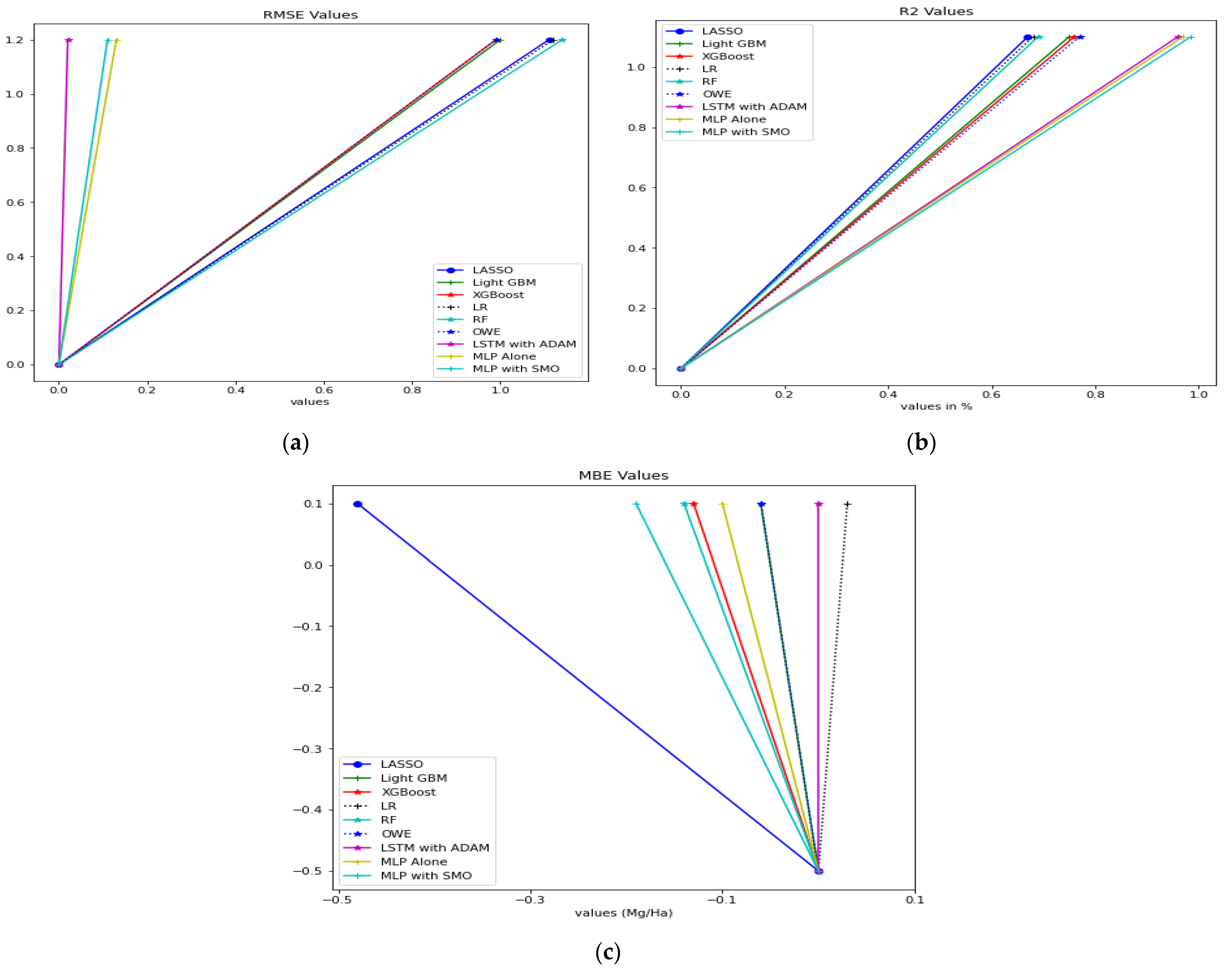
LASSO [34]	1.11	0.67	−0.48
LightGBM [34]	1.0	0.75	−0.06
XGBoost [34]	0.99	0.75	−0.13
RF [34]	1.12	0.68	−0.14
LR [34]	1.12	0.68	0.03
OWE [34]	0.99	0.75	−0.06
LSTM Model with Adam [54]	0.02	0.96
MLP alone	0.13	0.96	−0.10
MLP with SMO	0.11	0.98	−0.19

and the corresponding graphs are presented in Figure 7.

The above table demonstrates that the intended MLP with SMO has outperformed with minimal RMSE and higher R² values among the models that are being considered for statistical analysis. To make the model evident, the proposed model is also being evaluated concerning the mean absolute error, as shown in

Table 4. Performance comparison concerning RMSE, R², and MAE metrics.

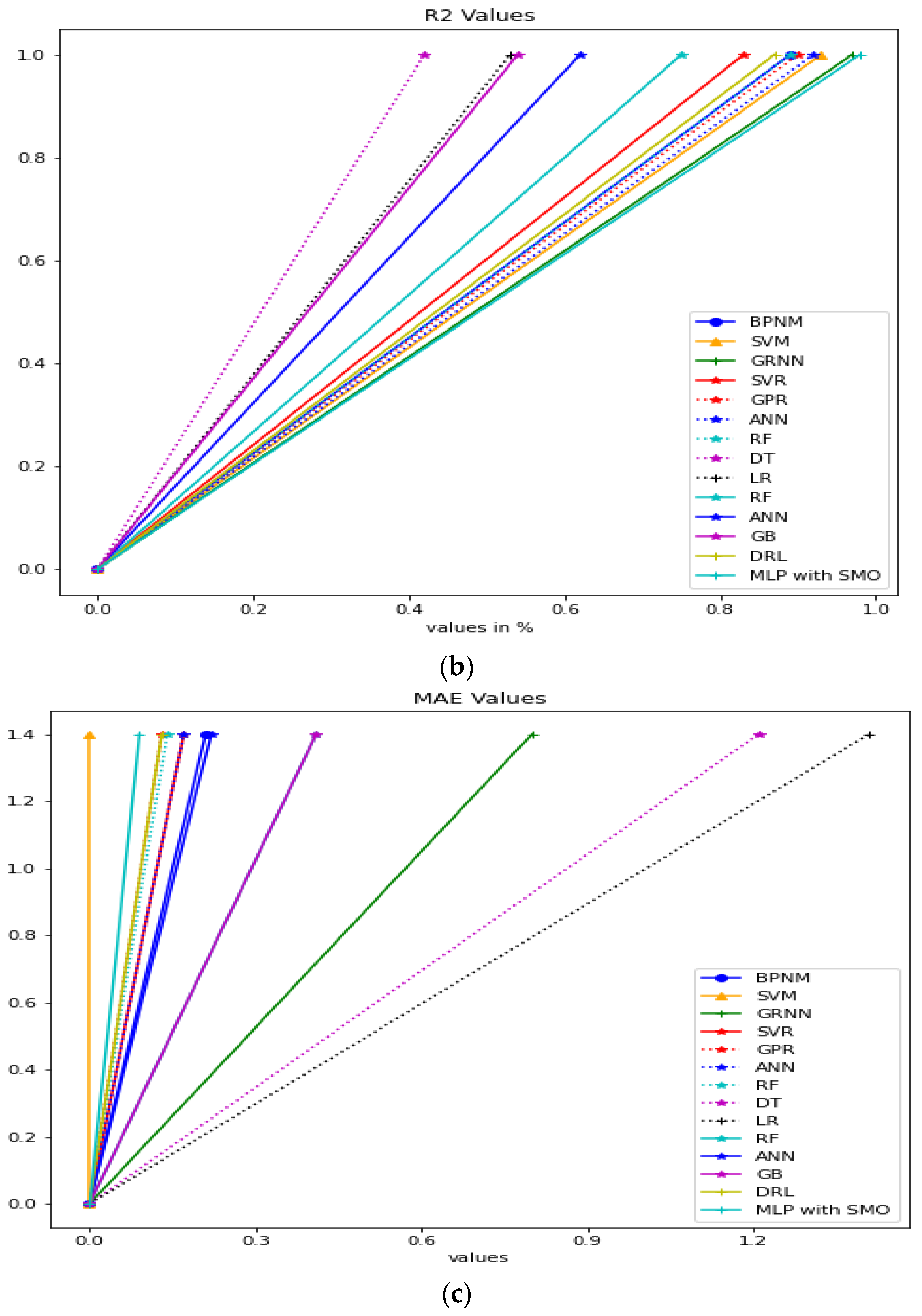
Approach	RMSE (Mg/Ha)	R2	MAE
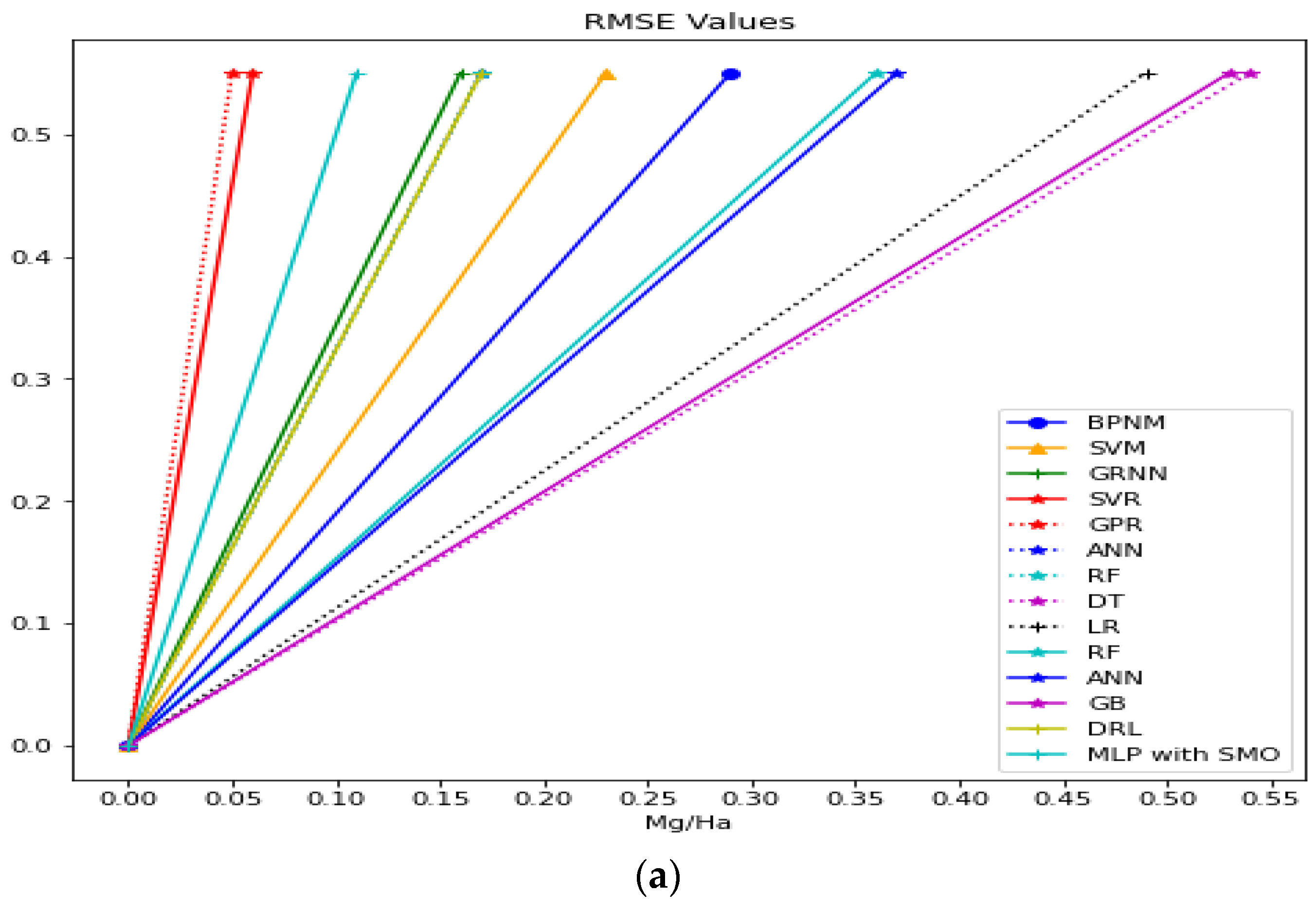
BPNM [38]	0.29	0.89	0.21
SVM [38]	0.23	0.93
GRNN [38]	0.16	0.97	0.08
SVR [55]	0.06	0.83	0.17
GPR [55]	0.05	0.90	0.13
ANN [55]	0.17	0.92	0.17
RF [55]	0.17	0.89	0.14
DT [56]	0.54	0.42	1.21
LR [56]	0.49	0.53	1.41
RF [56]	0.36	0.75	0.41
ANN [56]	0.37	0.62	0.22
Gradient Boosting [57]	0.53	0.54	0.41
DRL [57]	0.17	0.87	0.13
MLP with SMO	0.11	0.98	0.09

. The obtained values of the proposed approach and other state-of-the-art models are graphically represented in Figure 8.

It can be observed from the figures that are shown above, the proposed MLP with SMO model has resulted in minimal RMSE and MAE values compared to that of the other methods considered in the evaluation process. The model exhibited an exceptionally high R² value. The model is further evaluated using the 5-fold cross-validation for training RMSE, validation RMSE, training correlation, and validation correction percentages concerning the yield prediction for the MLP model alone and MLP with the SMO technique. The outcomes of the results are shown in

Table 5. Comparison of training and validation metrics of the proposed model.

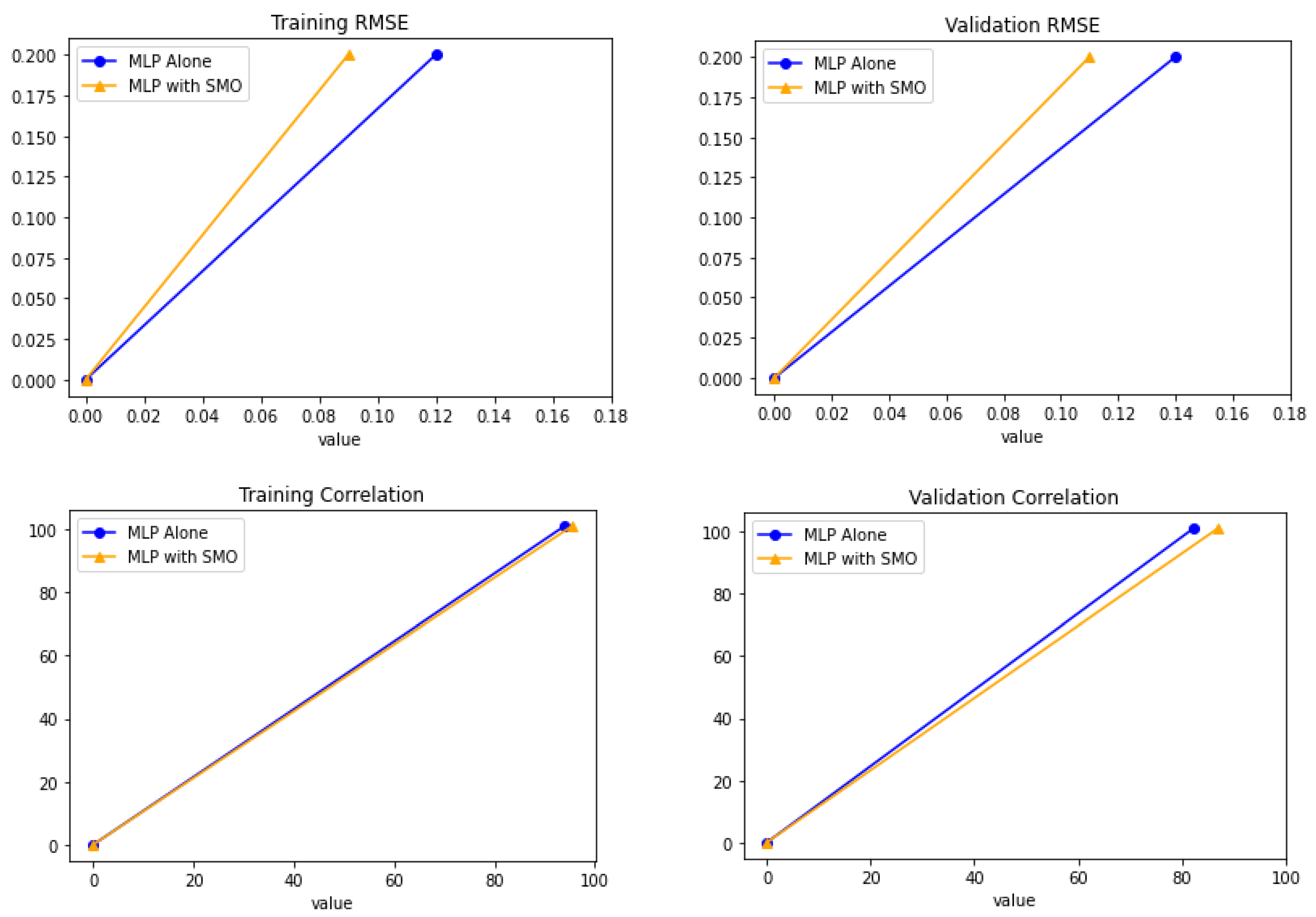
Approach	Training RMSE	Validation RMSE	Training Correlation	Validation Correlation
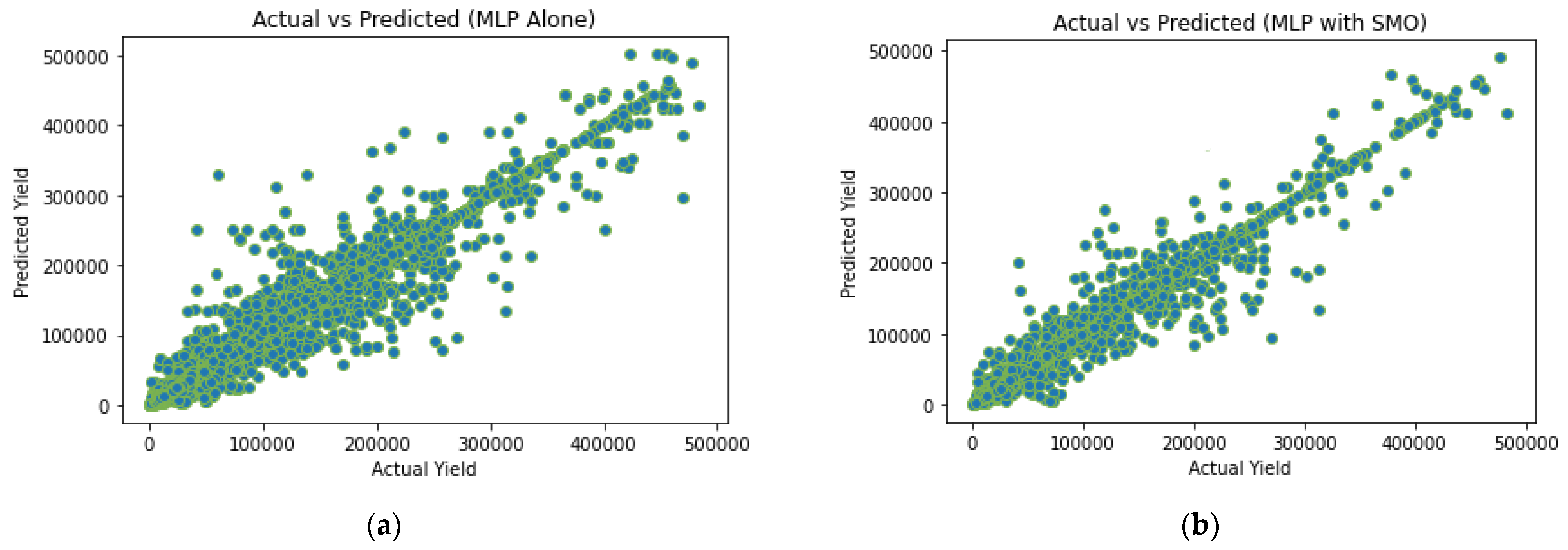
MLP	0.12	0.14	93.9%	82.2%
MLP with SMO	0.09	0.11	95.4%	86.9%

below, and the graphs generated are shown in Figure 9.

The proposed model is being further statistically analyzed using standard evaluation metrics such as the Wilcoxon signed-ranks test along with the wins and losses of the features that could be made to make the study more evident and explainable. The corresponding values of wins and losses with a standard deviation of 0.15 over 2139 records for MLP alone and MLP with SMO are presented in

Table 6. Wins and Loses instances with MLP and MLP with SMO.

	MLP	MLP with SMO
Wins (+)	2000	2061
Loses (−)	139	78

, and the Wilcoxon values are presented in

Table 7. Wilcoxon signed ranks for MLP and MLP with SMO.

	MLP	MLP with SMO
Average error	0.197	0.183
Average Fitness	0.271	0.259
Best Fitness	0.187	0.165
Worst Fitness	0.292	0.274
R+	51	51
R−	0	0
Significant(alpha)	0.05	0.05

.

The proposed approach has proven a reasonable efficiency concerning various evaluation parameters such as RMSE, R², MAE, MBE, and correlation. The current study’s statistical analysis is limited to the MLP model alone and MLP with SMO. The feature engineering process has not been considered in the evaluation process of divergent feature sets. The initial weights contributed to faster convergence of the model, but the impact of initial weights is not being analyzed in the current study. The current study is confined to the metrological factors that are being recorded in history, and the analysis is limited to recorded data. The changes that happen over the seasons and the crop demand for metrological changes as it keeps growing are not considered. Involving those underlying metrological factors might make the problem a complex temporal model, yet the models would yield a precise outcome in line with the changing scenarios.

The current model would work as a reference framework for crop yield prediction. Various studies on similar aspects working on machine models would assist the agriculture department, as the crop yield is largely dependent on the various factors that would change dynamically and would be challenging for precise predictions of the yield, even for the machine learning approaches. The other crucial factors are crop demand changes as it keeps growing, and the changes in metrological factors over the seasons and draught situations would keep the prediction models in a tough situation. There is a demand for sustainable models that take all the factors mentioned above into consideration.

6. Conclusions

The proposed study on the prediction of maize crop yield in the Saudi Arabia region using the Multi-Layer Perceptron model with Spider Monkey Optimization, the model has exhibited a promising performance in accurately forecasting the crop yield and evaluating the model with various metrics such as RMSE, R², MAE, and MBE the model has resulted in better performance than many states of art models. The proposed model makes predictions based on features such as average rainfall, average temperature, and Hg/Ha values in assessment. The data about the crop yield prediction would assist the farmers and the government in planning the imports and making the ecosystem ready for storing and processing the harvested crop. The model has exhibited a lower prediction error, with a reasonable training time. However, the proposed model has consumed a considerable amount of time for feature engineering, which could be considered one of the potential limitations of the proposed model, which has to be addressed in future studies.

Future studies can evaluate the model across divergent crops over distinct datasets. The number of features being considered for the yield analysis must be increased to increase the diverse factors. In contrast, in the current study, features such as fertilizer consumption, soil moisture, nutrition level, soil pH, water pH, and many other crucial features are not considered. There is a need to design intelligent machine models capable of working with minimal training, resulting in working with optimized resources. However, we think our study significantly contributes to the digital revolution in agriculture, helping us optimize agriculture and generate more with fewer resources. In future work, the metrological factors that would keep changing over the seasons and the demand for various underlying factors would result in a precise outcome. There is demand for models that could keep track of the changes in the crop as it keeps growing, as intermediator data is also crucial in making precision predictions.

References

- Al-Adhaileh, M.H.; Aldhyani, T.H. Artificial intelligence framework for modeling and predicting crop yield to enhance food security in Saudi Arabia. PeerJ Comput. Sci. 2022, 8, e1104. [Google Scholar] [CrossRef] [PubMed]
- Jayagopal, P.; Muthukumaran, V.; Koti, M.S.; Kumar, S.S.; Rajendran, S.; Mathivanan, S.K. Weather-based maize yield forecast in Saudi Arabia using statistical analysis and machine learning. Acta Geophys. 2022, 70, 2901–2916. [Google Scholar] [CrossRef]
- Elzaki, R.M.; Elrasheed, M.; Elmulthum, N.A. Optimal crop combination under soaring oil and energy prices in the kingdom of Saudi Arabia. Socio-Econ. Plan. Sci. 2022, 83, 101367. [Google Scholar] [CrossRef]
- Gana, R. Ridge Regression and the Elastic Net: How Do They Do as Finders of True Regressors and Their Coefficients? Mathematics 2022, 10, 3057. [Google Scholar] [CrossRef]
- Botana, I.L.-R.; Eiras-Franco, C.; Alonso-Betanzos, A. Regression Tree Based Explanation for Anomaly Detection Algorithm. Proceedings 2020, 54, 7. [Google Scholar] [CrossRef]
- Naga Srinivasu, P.; Srinivasa Rao, T.; Dicu, A.M.; Mnerie, C.A.; Olariu, I. A comparative review of optimisation techniques in segmentation of brain MR images. J. Intell. Fuzzy Syst. 2020, 38, 6031–6043. [Google Scholar] [CrossRef]
- Guleria, P.; Naga Srinivasu, P.; Ahmed, S.; Almusallam, N.; Alarfaj, F.K. XAI Framework for Cardiovascular Disease Prediction Using Classification Techniques. Electronics 2022, 11, 4086. [Google Scholar] [CrossRef]
- Nevavuori, P.; Narra, N.; Linna, P.; Lipping, T. Assessment of Crop Yield Prediction Capabilities of CNN Using Multisource Data. In New Developments and Environmental Applications of Drones; Lipping, T., Linna, P., Narra, N., Eds.; Springer: Cham, Switzerland, 2022. [Google Scholar] [CrossRef]
- Feng, P.; Wang, B.; Li Liu, D.; Waters, C.; Xiao, D.; Shi, L.; Yu, Q. Dynamic wheat yield forecasts are improved by a hybrid approach using a biophysical model and machine learning technique. Agric. For. Meteorol. 2020, 285–286, 107922. [Google Scholar] [CrossRef]
- Nyéki, A.; Neményi, M. Crop Yield Prediction in Precision Agriculture. Agronomy 2022, 12, 2460. [Google Scholar] [CrossRef]
- Yli-Heikkila, M.; Wittke, S.; Luotamo, M.; Puttonen, E.; Sulkava, M.; Pellikka, P.; Heiskanen, J.; Klami, A. Scalable Crop Yield Prediction with Sentinel-2 Time Series and Temporal Convolutional Network. Remote Sens. 2022, 14, 4193. [Google Scholar] [CrossRef]
- Khaki, S.; Wang, L. Crop yield prediction using deep neural networks. Front. Plant Sci. 2019, 10, 621. [Google Scholar] [CrossRef] [PubMed]
- Xu, J.; Tang, S.; Li, P.; Zhang, H. Empirical Study on the Grain Output Based on Regression Analysis. J. Sensors 2022, 2022, 2567790. [Google Scholar] [CrossRef]
- Shahhosseini, M.; Hu, G.; Huber, I.; Archontoulis, S.V. Coupling machine learning and crop modeling improves crop yield prediction in the US Corn Belt. Sci. Rep. 2021, 11, 1606. [Google Scholar] [CrossRef] [PubMed]
- Wang, X.; An, S.; Xu, Y.; Hou, H.; Chen, F.; Yang, Y.; Zhang, S.; Liu, R. A Back Propagation Neural Network Model Optimized by Mind Evolutionary Algorithm for Estimating Cd, Cr, and Pb Concentrations in Soils Using Vis-NIR Diffuse Reflectance Spectroscopy. Appl. Sci. 2020, 10, 51. [Google Scholar] [CrossRef]
- Maritz, J.; Lubbe, F.; Lagrange, L. A Practical Guide to Gaussian Process Regression for Energy Measurement and Verification within the Bayesian Framework. Energies 2018, 11, 935. [Google Scholar] [CrossRef]
- Guleria, P.; Ahmed, S.; Alhumam, A.; Srinivasu, P.N. Empirical Study on Classifiers for Earlier Prediction of COVID-19 Infection Cure and Death Rate in the Indian States. Healthcare 2022, 10, 85. [Google Scholar] [CrossRef]
- VGeetha, V.; Punitha, A.; Abarna, M.; Akshaya, M.; Illakiya, S.; Janani, A. An Effective Crop Prediction Using Random Forest Algorithm. In Proceedings of the 2020 International Conference on System, Computation, Automation, and Networking (ICSCAN), Puducherry, India, 3–4 July 2020; pp. 1–5. [Google Scholar] [CrossRef]
- Koduri, S.B.; Gunisetti, L.; Ramesh, C.R.; Mutyalu, K.V.; Ganesh, D. Prediction of crop production using adaboost regression method. J. Physics Conf. Ser. 2019, 1228, 012005. [Google Scholar] [CrossRef]
- Kopal, I.; Labaj, I.; Vršková, J.; Harničárová, M.; Valíček, J.; Ondrušová, D.; Krmela, J.; Palková, Z. A Generalized Regression Neural Network Model for Predicting the Curing Characteristics of Carbon Black-Filled Rubber Blends. Polymers 2022, 14, 653. [Google Scholar] [CrossRef]
- Bacanin, N.; Miodrag, Z.; Sarac, M.; Petrovic, A.; Strumberger, I.; Antonijevic, M.; Petrovic, A.; Venkatachalam, K.A.; Strumberger, I.; Antonijevic, M.; et al. A Novel Multiswarm Firefly Algorithm: An Application for Plant Classification. In Intelligent and Fuzzy Systems; Kahraman, C., Tolga, A.C., Cevik Onar, S., Cebi, S., Oztaysi, B., Sari, I.U., Eds.; INFUS 2022. Lecture Notes in Networks and Systems; Springer: Cham, Switzerland, 2022; Volume 504. [Google Scholar] [CrossRef]
- Haque, F.F.; Abdelgawad, A.; Yanambaka, V.P.; Yelamarthi, K. Crop Yield Prediction Using Deep Neural Network. In Proceedings of the 2020 IEEE 6th World Forum on Internet of Things (WF-IoT), New Orleans, LA, USA, 2–16 June 2020; pp. 1–4. [Google Scholar] [CrossRef]
- El-Kenawy, E.-S.M.; Khodadadi, N.; Mirjalili, S.; Makarovskikh, T.; Abotaleb, M.; Karim, F.K.; Alkahtani, H.K.; Abdelhamid, A.A.; Eid, M.M.; Horiuchi, T.; et al. Metaheuristic Optimization for Improving Weed Detection in Wheat Images Captured by Drones. Mathematics 2022, 10, 4421. [Google Scholar] [CrossRef]
- Oikonomidis, A.; Catal, C.; Kassahun, A. Hybrid Deep Learning-based Models for Crop Yield Prediction. Appl. Artif. Intell. 2022, 36, 1. [Google Scholar] [CrossRef]
- Batool, D.; Shahbaz, M.; Shahzad Asif, H.; Shaukat, K.; Alam, T.M.; Hameed, I.A.; Ramzan, Z.; Waheed, A.; Aljuaid, H.; Luo, S. A Hybrid Approach to Tea Crop Yield Prediction Using Simulation Models and Machine Learning. Plants 2022, 11, 1925. [Google Scholar] [CrossRef] [PubMed]
- Shingade, S.D.; Mudhalwadkar, R.P. Hybrid deep-Q Elman neural network for crop prediction and recommendation based on environmental changes. Concurr. Computat. Pract. Exper. 2022, 34, e6991. [Google Scholar] [CrossRef]
- Jambekar, S.; Nema, S.; Saquib, Z. Prediction of Crop Production in India Using Data Mining Techniques. In Proceedings of the Pune, Pune, India, 16–18 August 2018; pp. 1–5. [Google Scholar] [CrossRef]
- Vidhya, R.; Mathur, P.; Valluri, S.S. Crop yield prediction using random forest. Int. J. Adv. Sci. Technol. 2020, 29, 3084–3086. [Google Scholar]
- Sangeeta, S. Design and implementation of crop yield prediction model in agriculture. Int. J. Sci. Technol. Res. 2020, 8, 544–549. [Google Scholar]
- Deepalakshmi, P.; Prudhvi, K.T.; Siri, C.S.; Lavanya, K.; Srinivasu, P.N. Plant Leaf Disease Detection Using CNN Algorithm. Int. J. Inf. Syst. Model. Des. 2021, 12, 1–21. [Google Scholar] [CrossRef]
- You, J.; Li, X.; Low, M.; Lobell, D.; Ermon, S. Deep Gaussian process for crop yield prediction based on remote sensing data. In Proceedings of the Thirty-First AAAI Conference on Artificial Intelligence (AAAI’17); AAAI Press: Washington, DC, USA, 2017; pp. 4559–4565. [Google Scholar]
- Fegade, T.K.; Pawar, B. Crop Prediction Using Artificial Neural Network and Support Vector Machine. In Data Management, Analytics and Innovation; Springer: Berlin/Heidelberg, Germany, 2020; pp. 311–324. [Google Scholar]
- Tiwari, P.; Shukla, P.K. A hybrid approach of TLBO and EBPNN for crop yield prediction using spatial feature vectors. J. Artif. Intell. 2019, 1, 45–59. [Google Scholar] [CrossRef]
- Sajid, S.S.; Shahhosseini, M.; Huber, I.; Hu, G.; Archontoulis, S.V. County-scale crop yield prediction by integrating crop simulation with machine learning models. Front. Plant Sci. 2022, 13, 1000224. [Google Scholar] [CrossRef]
- Krithika, K.M.; Maheswari, N.; Sivagami, M. Models for feature selection and efficient crop yield prediction in the groundnut production. Res. Agric. Eng. 2022, 68, 131–141. [Google Scholar] [CrossRef]
- Ikram, A.; Aslam, W.; Aziz, R.H.H.; Noor, F.; Mallah, G.A.; Ikram, S.; Ahmad, M.S.; Abdullah, A.M.; Ullah, I. Crop Yield Maximization Using an IoT-Based Smart Decision. J. Sens. 2022, 2022, 2022923. [Google Scholar] [CrossRef]
- Kumar, R. IoT Enabled Crop Prediction and Irrigation Automation System Using Machine Learning. Recent Adv. Comput. Sci. Commun. 2022, 15, 88–97. [Google Scholar] [CrossRef]
- Joshua, S.V.; Priyadharson, A.S.M.; Kannadasan, R.; Khan, A.A.; Lawanont, W.; Khan, F.A.; Rehman, A.U.; Ali, M.J. Crop yield prediction using machine learning approaches on a wide spectrum. Comput. Mater. Contin. 2022, 72, 5663–5679. [Google Scholar]
- Vignesh, K.; Askarunisa, A.; Abirami, A.M. Optimized Deep Learning Methods for Crop Yield Prediction. Comput. Syst. Sci. Eng. 2023, 44, 1051–1067. [Google Scholar] [CrossRef]
- Paudel, D.; Boogaard, H.; de Wit, A.; Janssen, S.; Osinga, S.; Pylianidis, C.; Athanasiadis, I.N. Machine learning for large-scale crop yield forecasting. Agric. Syst. 2020, 187, 103016. [Google Scholar] [CrossRef]
- Bali, N.; Singla, A. Deep Learning Based Wheat Crop Yield Prediction Model in Punjab Region of North India. Appl. Artif. Intell. 2021, 35, 1304–1328. [Google Scholar] [CrossRef]
- Rajagopal, A.; Jha, S.; Khari, M.; Ahmad, S.; Alouffi, B.; Alharbi, A. A Novel Approach in Prediction of Crop Production Using Recurrent Cuckoo Search Optimization Neural Networks. Appl. Sci. 2021, 11, 9816. [Google Scholar] [CrossRef]
- Ansarifar, J.; Wang, L.; Archontoulis, S.V. An interaction regression model for crop yield prediction. Sci. Rep. 2021, 11, 17754. [Google Scholar] [CrossRef]
- Uddin, M.F.; Lee, J.; Rizvi, S.; Hamada, S. Proposing Enhanced Feature Engineering and a Selection Model for Machine Learning Processes. Appl. Sci. 2018, 8, 646. [Google Scholar] [CrossRef]
- Lee, C.-H.; Gutierrez, F.; Dou, D. Calculating Feature Weights in Naive Bayes with Kullback-Leibler Measure. In Proceedings of the 2011 IEEE 11th International Conference on Data Mining, Vancouver, BC, Canada, 11 December 2011; pp. 1146–1151. [Google Scholar] [CrossRef]
- Isabona, J.; Imoize, A.L.; Ojo, S.; Karunwi, O.; Kim, Y.; Lee, C.-C.; Li, C.-T. Development of a Multilayer Perceptron Neural Network for Optimal Predictive Modeling in Urban Microcellular Radio Environments. Appl. Sci. 2022, 12, 5713. [Google Scholar] [CrossRef]
- Rojas, M.G.; Olivera, A.C.; Vidal, P.J. Optimising Multilayer Perceptron weights and biases through a Cellular Genetic Algorithm for medical data classification. Array 2022, 14, 100173. [Google Scholar] [CrossRef]
- Ethala, S.; Kumarappan, A. A Hybrid Spider Monkey and Hierarchical Particle Swarm Optimization Approach for Intrusion Detection on Internet of Things. Sensors 2022, 22, 8566. [Google Scholar] [CrossRef]
- Crop Yield Prediction Dataset. Available online: https://www.kaggle.com/datasets/patelris/crop-yield-prediction-dataset (accessed on 25 December 2022).
- Food and Agriculture Organization. Available online: http://www.fao.org/home/en/ (accessed on 25 December 2022).
- World Data Bank. Available online: https://data.worldbank.org/ (accessed on 25 December 2022).
- Derrac, J.; García, S.; Molina, D.; Herrera, F. A practical tutorial on the use of nonparametric statistical tests as a methodology for comparing evolutionary and swarm intelligence algorithms. Swarm Evol. Comput. 2011, 1, 3–18. [Google Scholar] [CrossRef]
- Srinivasu, N.P.; Rao, S.T.; Srinivas, G.; Reddy, P.P.V.G.D. A Computationally Efficient Skull Scraping Approach for Brain MR Image. Recent Adv. Comput. Sci. Commun. 2020, 13, 833–844. [Google Scholar] [CrossRef]
- Çetiner, H.; Kara, B. Recurrent Neural Network based model development for wheat yield forecasting. Adıyaman Üniversitesi Mühendislik Bilim. Derg. 2022, 9, 204–218. [Google Scholar] [CrossRef]
- Ahmed, N.; Asif, H.; Saleem, G.; Muhammad, M. Development of Crop Yield Estimation Model using Soil and Environmental Parameters. arXiv preprint 2021, arXiv:2102.05755. [Google Scholar] [CrossRef]
- Chicco, D.; Warrens, M.J.; Jurman, G. The coefficient of determination R-squared is more informative than SMAPE, MAE, MAPE, MSE and RMSE in regression analysis evaluation. PeerJ Comput. Sci. 2021, 7, e623. [Google Scholar] [CrossRef] [PubMed]
- Elavarasan, D.; Vincent, P.M.D. Crop Yield Prediction Using Deep Reinforcement Learning Model for Sustainable Agrarian Applications. IEEE Access 2020, 8, 86886–86901. [Google Scholar] [CrossRef]