Missing Structural Health Monitoring Data Recovery Based on Bayesian Matrix Factorization

Abstract

The exposure of bridge health-monitoring systems to extreme conditions often results in missing data, which constrains the health monitoring system from working. Therefore, there is an urgent need for an efficient data cleaning method. With the development of big data and machine-learning techniques, several methods for missing-data recovery have emerged. However, optimization-based methods may experience overfitting and demand extensive tuning of parameters, and trained models may still have substantial errors when applied to unseen datasets. Furthermore, many methods can only process monitoring data from a single sensor at a time, so the spatiotemporal dependence among monitoring data from different sensors cannot be extracted to recover missing data. Monitoring data from multiple sensors can be organized in the form of matrix. Therefore, matrix factorization is an appropriate way to handle monitoring data. To this end, a hierarchical probabilistic model for matrix factorization is formulated under a fully Bayesian framework by incorporating a sparsity-inducing prior over spatiotemporal factors. The spatiotemporal dependence is modeled to reconstruct the monitoring data matrix to achieve the missing-data recovery. Through experiments using continuous monitoring data of an in-service bridge, the proposed method shows good performance of missing-data recovery. Furthermore, the effect of missing data on the preset rank of matrix is also investigated. The results show that the model can achieve higher accuracy of missing-data recovery with higher preset rank under the same case of missing data.

1. Introduction

With the expansion of the global economy, there is a corresponding worldwide increase in the number of infrastructure constructions, particularly large bridges. However, structural damage to bridges can lead to devastating disasters. Therefore, structural health monitoring (SHM) of bridges is of paramount importance. High-quality data form the foundation of SHM systems [1]. Nevertheless, the monitoring data inevitably contain missing data because of the harsh and noisy environments in which the SHM system operates. Therefore, the recovery of missing data is imminent [2].

With the development of data acquisition technology, SHM is facing big data problem, such as missing recovery and damage identification [3], which needs to be solved with machine learning and deep learning approaches. There have been numerous efforts in SHM targeting missing-data recovery. Missing-data recovery is using observed data to restore missing data. Therefore, non-destructive methods based on the use of data mining approaches are very appropriate to restore missing data. Many scholars have proposed various non-destructive methods based on the use of data mining approaches for missing recovery, including traditional machine learning and novel deep learning. On the one hand, due to the powerful nonlinear fitting ability of neural networks, neural networks have been used for missing-data recovery and achieved good results. Jeong et al. [4] used a bidirectional recurrent neural network (RNN) to develop a method for monitoring data recovery applied to SHM. Liu [5] et al. recovered missing data using long short-term memory (LSTM). Rautela et al. [6] used model assisted convolutional and recurrent neural networks to realize structural damage detection and localization. The results showed that both the networks have good performance of classification and regression. However, in practical engineering, high-quality datasets for training neural networks are not readily available. On the other hand, because of the uncertainty of monitoring data, probabilistic methods are natural methods for missing data restoration. For example, Wan et al. [7] used Bayesian multitask learning with multidimensional GP priors to recover missing data. Chen [8] used functional data analysis techniques to analyze and model the inter-sensor relationship between the two strain sensors located at different locations. However, model selection is time-consuming. Rabcan et al. [9] proposed non-destructive diagnostic of aircraft engine blades by fuzzy decision tree, which also can be used to solve regression problems, such as missing-data recovery.

However, some unignorable challenges still exist in the research of missing-data recovery. First, as mentioned above, high-quality datasets for training neural networks are often difficult to obtain because of the ubiquity of missing data. Second, tuning the parameters is also very time-consuming during training deep neural networks, which limits the application of deep learning in recovery of missing data. Finally, traditional machine learning, such as support vector machine (SVM), can only achieve recovery of missing data from a single sensor. However, each sensor may contain missing data in its monitoring data. There are also other problems in some machine learning algorithms. For example, decision tree as a predictive model has been used to solve classification and regression problems in structure engineering and achieved good results. However, it is prone to overfitting when used for regression problems such as missing-data recovery. The utilization of tensor learning has been employed to make substantial advances in image processing, recommender systems, and traffic data analysis [10,11,12,13,14], yielding a resurgence in recent years, which may be one of the solutions to the above challenges. It has been shown that tensor learning can be applied to missing SHM data recovery [15]. Specifically, multisource monitoring data can be organized as matrices (i.e., low-rank tensors). Spatiotemporal matrix factorization is then applied, where the low-rank structure can effectively describe the complicated spatiotemporal dependence based on the data to obtain the spatiotemporal feature factors of the monitoring-data matrix. Based on the spatiotemporal feature factors, the entire monitoring-data matrix can be reconstructed, and the missing data can be recovered during reconstruction.

Compared to deep learning and traditional machine learning, tensor learning has the ability to deal with sparse and incomplete data [16]. Therefore, tensor learning can recover missing data without high quality datasets. Furthermore, we developed an efficient deterministic Bayesian inference algorithm for matrix factorization, which solves problems of tuning and overfitting. Last but not least, matrix factorization can extract the spatio-temporal dependence in monitoring data and recover missing data from multiple sensors simultaneously, greatly improving the efficiency of missing recovery.

The main contributions of this study are as follows: first, missing data in monitoring data from all sensors are restored simultaneously by extracting the spatiotemporal characteristics of the monitoring-data matrix. Second, the entire model is placed in a full Bayesian framework, which solves the problem of overfitting and tuning. Finally, we achieve recovery of missing data using low-quality dataset directly.

The main contents of this study are as follows. The introduction is presented in the first section of this paper. The Bayesian matrix factorization (BMF) theory used in this study is described in Section 2. In Section 2.1, the general principles of the missing-data recovery problem are introduced. In Section 3, the performance of the proposed method is verified using actual engineering monitoring data. Section 4 summarizes the main contributions of this study and proposes future research prospects.

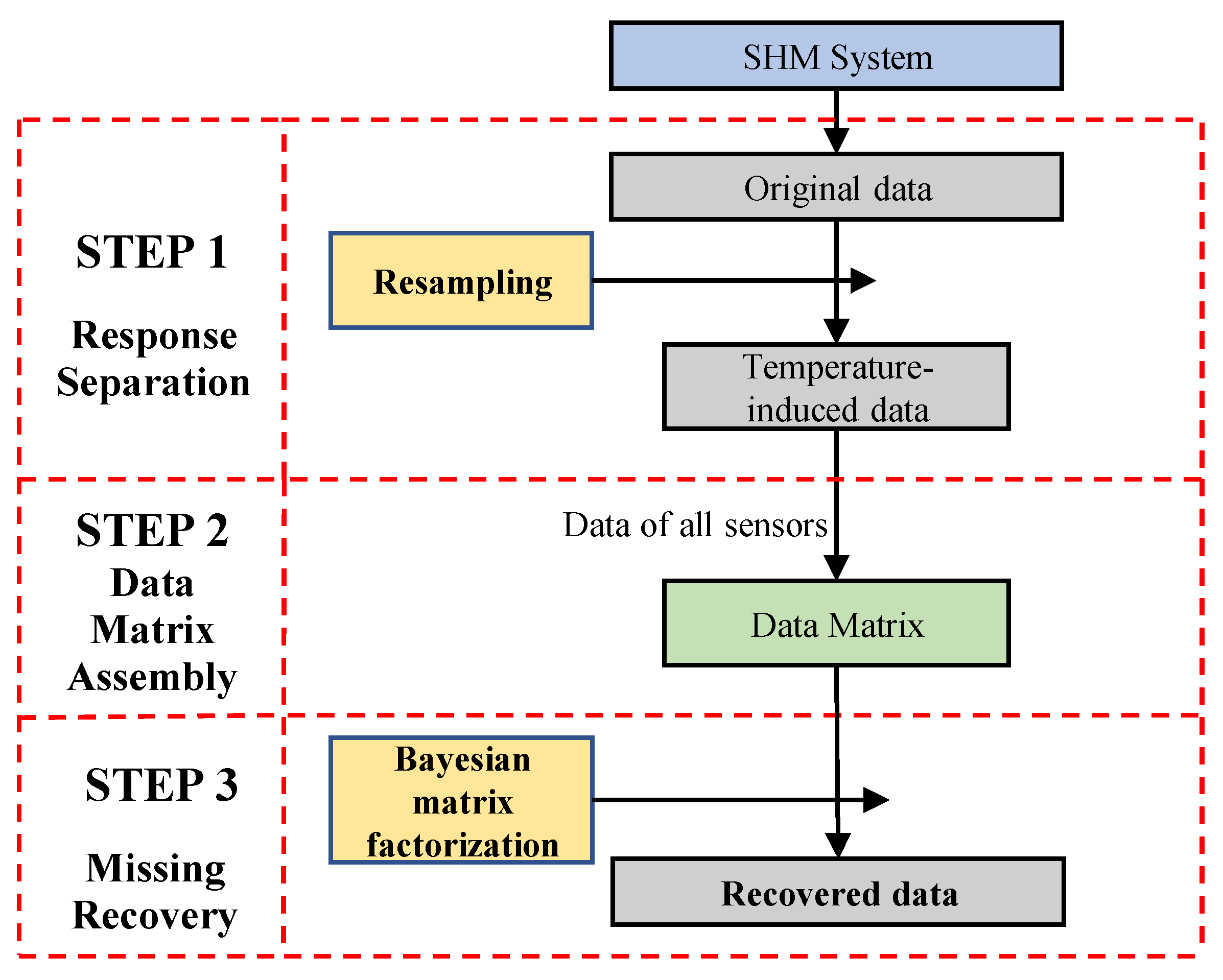
2. Methodology

In this section, the problem of missing-data recovery for SHM systems based on Bayesian matrix factorization is elaborated, and the theoretical model and methodology are introduced in detail.

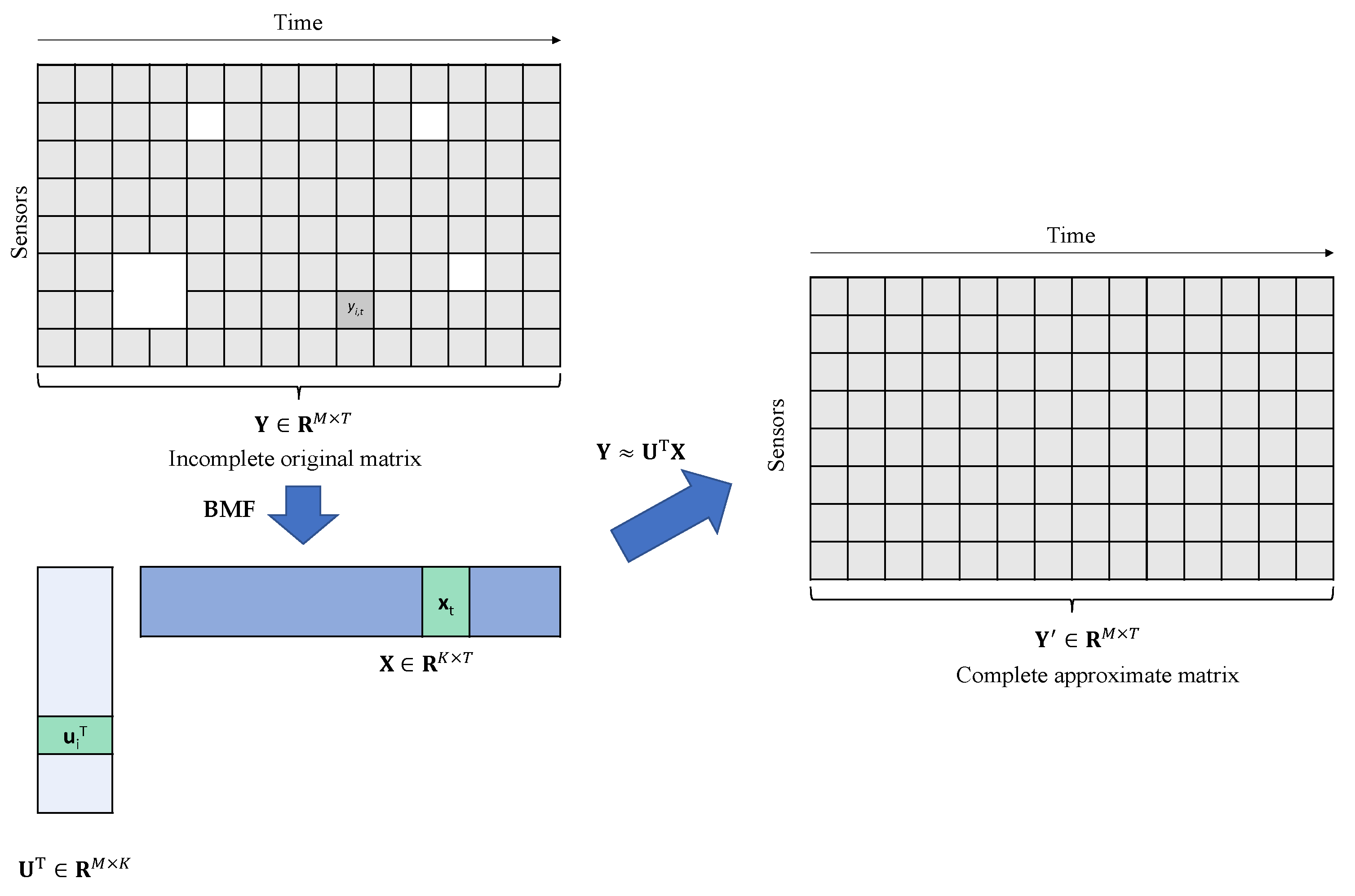
2.1. Problem Introduction

The aim of missing-data recovery is to attain the missing data by utilizing the data obtained from the sensors through monitoring [17]. The multisource monitoring data containing missing data can be organized in the form of a matrix $Y\in R^{\mathrm{M}\times \mathrm{T}}$, where M is the number of sensors and T is the number of timestamps during a continuous monitoring period. The missing recovery process first learns the spatial factor U and temporal factor X from observation Y containing the missing data. Missing recovery can then be achieved using the learned spatial factor U and temporal factor X to obtain the approximate and complete matrix.

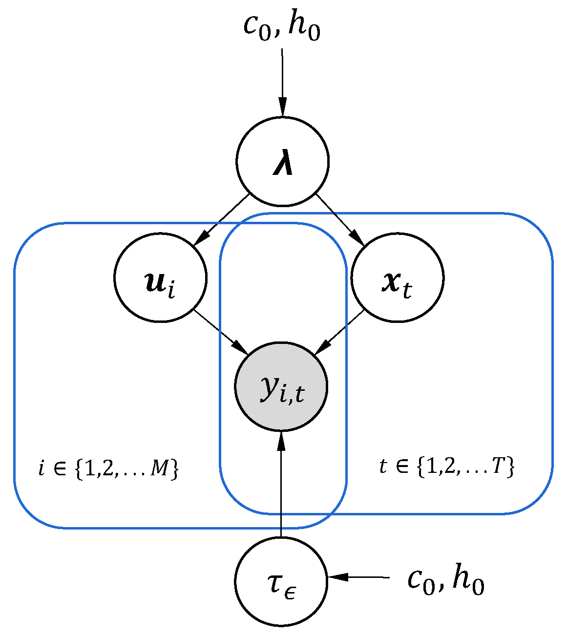
2.2. Bayesian Hierarchical Model for Matrix Factorization

The SHM data with T timestamps observed from M sensors can be constructed in the form of a matrix: $Y\in R^{\mathrm{M}\times \mathrm{T}}$. Because there are inevitable missing data in practice, an indicator set B for the elements observed in Y is set to indicate the location of missing data in the observed data Y, that is, if $y_{i,t}$ is missing, then $b_{i,j}=0$ else, $b_{i,j}=0$. To characterize the spatiotemporal dependence, we use matrix factorization to approximate the observations using two-factor matrices:

$$Y\approx U^{\mathrm{T}}X$$

(1)

where $U\in R^{\mathrm{K}\times \mathrm{M}}$ denotes a potential spatial factor whose column vector is ${\mathrm{u}}_{\mathrm{i}}$; $X\in R^{\mathrm{K}\times \mathrm{M}}$ denotes the potential temporal factor whose column vector is $x_{\mathrm{t}}$, where K denotes the rank of the matrix. ${\mathrm{y}}_{\mathrm{i},\mathrm{t}}$ is obtained from the inner product of $u_{\mathrm{i}}$ and $x_{\mathrm{t}}$,

$${\mathrm{y}}_{\mathrm{i},\mathrm{t}}\approx u_{\mathrm{i}}^{\mathrm{T}}{x}_{\mathrm{t}},$$

(2)

where $u_{\mathrm{i}}$∈$R^{\mathrm{K}}$ denotes the latent spatial feature of the ith sensor and $x_{\mathrm{t}}\in R^{\mathrm{K}}$ is the latent temporal feature bound to time t. The schematic of the robust matrix factorization is shown in Figure 1, which illustrates that the purpose of matrix factorization is to achieve missing recovery in the process of data reconstruction using learnt spatial and temporal factors.

As mentioned above, we employ a fully Bayesian treatment for matrix factorization to solve problems of overfitting and tuning. The probabilistic graphical model of Bayesian matrix factorization proposed in this study is shown in Figure 2. The Bayesian inference process shown in Figure 2 is described in detail as follow.

2.3. Setting Priors for Parameters and Hyperparameters

The process of modeling a fully Bayesian approach for matrix factorization is described in detail. First, we assume that the prior distribution of observations ${\mathrm{y}}_{\mathrm{i},\mathrm{t}}$ is a Gaussian distribution, that is,

$${\mathrm{y}}_{\mathrm{i},\mathrm{t}}~\mathrm{N}\left(u_{\mathrm{i}}^{\mathrm{T}}{x}_{\mathrm{t}},{\mathsf{\tau }}_{ϵ}^{-1}\right),$$

(3)

where $\mathrm{N}(·)$ denotes the Gaussian distribution and ${\mathsf{\tau }}_{ϵ}$ is the precision term.

Next, we model the spatial feature $u_{\mathrm{i}}$ and the temporal feature $x_{\mathrm{t}}$. A multivariate normal distribution is placed on both spatial feature $u_{\mathrm{i}}$ and temporal feature $x_{\mathrm{t}}$, that is,

$$u_{\mathrm{i}}~\mathrm{N}\left(\mathbf{0},{\left[\mathrm{diag}\left(\lambda \right)\right]}^{-1}\right),$$

(4)

$$x_{\mathrm{t}}~\mathrm{N}\left(\mathbf{0},{\left[\mathrm{diag}\left(\lambda \right)\right]}^{-1}\right),$$

(5)

where $\mathbf{0}\in R^{\mathrm{K}}$ denotes the mean vector. The purpose of setting the mean vector to zero is to simplify the structure of the Bayesian network. $\mathrm{diag}(·)$ denotes diagonalization of the matrix. $\lambda \in R^{\mathrm{K}}$ is the hyperparameter of the spatiotemporal features $u_{\mathrm{i}}$ and $x_{\mathrm{t}}$, whose diagonalized matrix can then be transformed into a multivariate normally distributed covariance matrix.

The next stage of Bayesian model generation is modeling the hyperparameter λ and the precision term ${\mathsf{\tau }}_{ϵ}$. First, we modeled the hyperparameter λ. To make the covariance matrix of multivariate normal distribution positive definite, each element of λ should always be positive. Therefore, we assumed that the prior distribution of all elements in vector λ is a gamma distribution, that is,

$${\mathsf{\lambda }}_{\mathrm{j}}~\mathrm{Gamma}\left({\mathrm{c}}_0,{\mathrm{h}}_0\right),\mathrm{j}\in \left\{1,2,\dots ,\mathrm{K}\right\}.$$

(6)

Subsequently, we placed the gamma distribution on ${\mathsf{\tau }}_{ϵ}$ as its prior distribution, that is,

$${\mathsf{\tau }}_{ϵ}~\mathrm{Gamma}\left({\mathrm{a}}_0,{\mathrm{b}}_0\right),$$

(7)

where the gamma distribution probability density formula is

$$\mathrm{p}({\mathsf{\tau }}_{ϵ}{|\mathrm{a}}_0,{\mathrm{b}}_0)=\frac{{\mathrm{b}}_0{}^{{\mathrm{a}}_0}}{\mathsf{\Gamma }({\mathrm{a}}_0)}{({\mathsf{\tau }}_{ϵ})}^{{\mathrm{a}}_0-1}\exp (-{\mathrm{b}}_0{\mathsf{\tau }}_{ϵ}),$$

(8)

where ${\mathrm{a}}_0$ is shape parameter and ${\mathrm{b}}_0$ is rate parameter.

2.4. Gibbs Sampling for Bayesian Matrix Factorization

After setting priors for parameters and hyperparameters, we can use the model to obtain the predicted distribution of missing data. Based on the Bayesian modeling formulation, the predicted distribution of missing data is inferred as follows:

$$\mathrm{p}\left({\mathrm{y}}_{\mathrm{i},\mathrm{t}}^{*}|Y,{\mathrm{a}}_0,{\mathrm{b}}_0,{\mathrm{c}}_0,{\mathrm{h}}_0\right)={\displaystyle \int }{\displaystyle \int }\mathrm{p}\left({\mathrm{y}}_{\mathrm{i},\mathrm{t}}^{*}|u_{\mathrm{i}},x_{\mathrm{t}},{\mathsf{\tau }}_{ϵ}\right)\mathrm{p}\left(U,X,{\mathsf{\tau }}_{ϵ}|Y,\lambda ,{\mathrm{c}}_0,{\mathrm{h}}_0\right)\mathrm{p}\left(\lambda {|\mathrm{a}}_0,{\mathrm{b}}_0\right)\mathrm{d}\left\{U,X,{\mathsf{\tau }}_{ϵ}\right\}\mathrm{d}\left\{\lambda \right\}.$$

(9)

However, because the integral in Equation (9) is extremely complex, its exact analytical solution cannot be obtained. Thus far, we use MCMC sampling to determine the approximate solution to Equation (9). The basic principle of MCMC sampling is that independent sample sequences can be drawn from the target distribution to approximate the entire distribution. The approximate solution to the predictive distribution in Equation (9) can be expressed as follows:

$$\mathrm{p}\left({\mathrm{y}}_{\mathrm{i},\mathrm{t}}^{*}|Y,{\mathrm{a}}_0,{\mathrm{b}}_0,{\mathrm{c}}_0,{\mathrm{h}}_0\right)\approx \frac{1}{\mathrm{N}}{\displaystyle \sum }_{\mathrm{n}=1}^{\mathrm{N}}\mathrm{p}\left({\mathrm{y}}_{\mathrm{i},\mathrm{t}}^{*}|u_{\mathrm{i}}^{\left(\mathrm{n}\right)},x_{\mathrm{t}}^{\left(\mathrm{n}\right)},{\mathsf{\tau }}_{ϵ}^{\left(\mathrm{n}\right)}\right),$$

(10)

where $\{u_{\mathrm{i}}^{\left(\mathrm{n}\right)},x_{\mathrm{t}}^{\left(\mathrm{n}\right)},{\mathsf{\tau }}_{ϵ}^{\left(\mathrm{n}\right)}\}$ denotes the sample obtained from the nth sampling of the target’s posterior distribution. In this study, we used Gibbs sampling to sample the target distribution. Gibbs sampling is a special branch of MCMC sampling for high-dimensional distributions, in which each variable is sampled from its conditional distribution while keeping other variables fixed. Next, we describe the Gibbs sampling process for each parameter in Bayesian matrix factorization in detail.

2.4.1. Sampling Spatiotemporal Feature ${\mathrm{u}}_{\mathrm{i}}$ and ${\mathrm{x}}_{\mathrm{t}}$

According to Bayes’ rule, likelihood function in Equation (3), prior distribution in Equation (4), and posterior distribution of the spatial feature, $u_{\mathrm{i}}$ can be obtained as

$$\mathrm{p}\left({\mathsf{\mu }}_{\mathrm{i}}|x_{\mathrm{t}},U,{\mathsf{\tau }}_{ϵ},\lambda \right)=\mathrm{N}\left({\mathsf{\mu }}_{\mathrm{i}}|{\tilde{\mathsf{\mu }}}_{\mathrm{i}}^{*},{\tilde{\Lambda }}_{\mathrm{i}}^{*}\right)\propto {\displaystyle \prod }_{\mathrm{t}=1}^{\mathrm{T}}\mathrm{N}\left({\mathrm{y}}_{\mathrm{i},\mathrm{t}}|u_{\mathrm{i}}^{\mathrm{T}}{x}_{\mathrm{t}},{\mathsf{\tau }}_{ϵ}\right)\times \left(u_{\mathrm{i}}|\mathbf{0},{\left[\mathrm{diag}\left(\lambda \right)\right]}^{-1}\right).$$

(11)

Let $A_{\mathrm{i}}=b_{\mathrm{i}}{}^{\mathrm{T}}\odot X^{\mathrm{T}}$, where ⊙ denotes the Khatri–Rao product, then

$${\tilde{\Lambda }}_{\mathrm{i}}^{*}={\left[{\mathsf{\tau }}_{ϵ}{A}_{\mathrm{i}}{A}_{\mathrm{i}}{}^{\mathrm{T}}\right]}^{-1},{\tilde{\mathsf{\mu }}}_{\mathrm{i}}^{*}={\mathsf{\tau }}_{ϵ}{\tilde{\Lambda }}_{\mathrm{i}}^{*}{A}_{\mathrm{i}}{y}_{\mathrm{i}}.$$

(12)

The posterior distribution of the temporal feature $x_{\mathrm{t}}$ can be obtained in a similar manner. According to Bayes’ rule, the posterior distribution of the temporal feature $x_{\mathrm{t}}$ can be expressed as follows:

$$\mathrm{p}\left(x_{\mathrm{t}}|u_{\mathrm{i}},X,{\mathsf{\tau }}_{ϵ},\lambda \right)=\mathrm{N}\left(x_{\mathrm{t}}|{\tilde{x}}_{\mathrm{t}}^{*},{\tilde{\Lambda }}_{\mathrm{t}}^{*}\right)\propto {{\displaystyle \prod }}_{\mathrm{i}=1}^{\mathrm{M}}\mathrm{N}\left({\mathrm{y}}_{\mathrm{i},\mathrm{t}}|u_{\mathrm{i}}^{\mathrm{T}}{x}_{\mathrm{t}},{\mathsf{\tau }}_{ϵ}\right)\times \left(x_{\mathrm{t}}|0,{\left[\mathrm{diag}\left(\lambda \right)\right]}^{-1}\right).$$

(13)

Let $A_{\mathrm{i}}=b_{\mathrm{i}}{}^{\mathrm{T}}\odot U^{\mathrm{T}}$, then

$${\tilde{\Lambda }}_{\mathrm{t}}^{*}={\left[{\mathsf{\tau }}_{ϵ}{A}_{\mathrm{t}}{A}_{\mathrm{t}}{}^{\mathrm{T}}\right]}^{-1},{\tilde{x}}_{\mathrm{t}}^{*}={\mathsf{\tau }}_{ϵ}{\tilde{\Lambda }}_{\mathrm{t}}^{*}{A}_{\mathrm{t}}{y}_{\mathrm{t}}.$$

(14)

2.4.2. Sampling ${\mathsf{\tau }}_{ϵ}$

According to Bayes’ rule, we can obtain the posterior distribution of the accuracy term ${\mathsf{\tau }}_{ϵ}$:

$$\mathrm{p}\left({\mathsf{\tau }}_{ϵ}{|\mathrm{y}}_{\mathrm{i},\mathrm{t}},x_{\mathrm{t}},u_{\mathrm{i}},{\mathsf{\tau }}_{ϵ},{\mathrm{a}}_0,{\mathrm{b}}_0\right)=\mathrm{Gamma}\left({\mathsf{\tau }}_{ϵ}|{\tilde{\mathrm{a}}}_0^{*},{\tilde{\mathrm{b}}}_0^{*}\right)\propto {\displaystyle \prod }_{\mathrm{i}=1}^{\mathrm{M}}{\displaystyle \prod }_{\mathrm{t}=1}^{\mathrm{T}}{\mathrm{b}}_{\mathrm{i},\mathrm{t}}\left({\mathrm{y}}_{\mathrm{i},\mathrm{t}}|u_{\mathrm{i}}^{\mathrm{T}}{x}_{\mathrm{t}},{\mathsf{\tau }}_{ϵ}\right)\times \mathrm{Gamma}\left({\mathrm{a}}_0,{\mathrm{b}}_0\right),$$

(15)

where

$${\tilde{\mathrm{a}}}_0^{*}={\mathrm{a}}_0+\frac{1}{2}{{\displaystyle \sum }}_{\mathrm{i},\mathrm{t}}{\mathrm{b}}_{\mathrm{i},\mathrm{t}},{\tilde{\mathrm{b}}}_0^{*}={\mathrm{b}}_0+\frac{1}{2}{{\displaystyle \sum }}_{\mathrm{i},\mathrm{t}}{\mathrm{b}}_{\mathrm{i},\mathrm{t}}\left({\mathrm{y}}_{\mathrm{i},\mathrm{t}}-u_{\mathrm{i}}^{\mathrm{T}}{x}_{\mathrm{t}}\right).$$

(16)

2.4.3. Sampling Hyperparameter λ

The posterior distribution of the hyperparameter λ is as follows:

$$\mathrm{p}\left({\mathsf{\lambda }}_{\mathrm{j}}|U,X,{\mathrm{c}}_0,{\mathrm{h}}_0\right)=\mathrm{Gamma}\left({\mathsf{\lambda }}_{\mathrm{j}}|{\tilde{\mathrm{c}}}_0^{*},{\tilde{\mathrm{h}}}_0^{*}\right)\propto {\displaystyle \prod }_{\mathrm{i}=1}^{\mathrm{M}}\mathrm{p}\left({\mathrm{u}}_{\mathrm{ij}}{|\mathsf{\lambda }}_{\mathrm{j}}\right){\displaystyle \prod }_{\mathrm{t}=1}^{\mathrm{T}}\mathrm{p}\left({\mathrm{x}}_{\mathrm{tj}}{|\mathsf{\lambda }}_{\mathrm{j}}\right)\times \mathrm{Gamma}\left({\mathrm{c}}_0,{\mathrm{h}}_0\right),$$

(17)

where

$${\tilde{\mathrm{c}}}_0^{*}={\mathrm{c}}_0+\frac{1}{2}\left(\mathrm{M}+\mathrm{T}\right),{\tilde{\mathrm{h}}}_0^{*}={\mathrm{h}}_0+\frac{1}{2}\left({\displaystyle \sum }_{\mathrm{i}=1}^{\mathrm{M}}{\mathrm{u}}_{\mathrm{ij}}{}^2+{\displaystyle \sum }_{\mathrm{t}=1}^{\mathrm{T}}{\mathrm{x}}_{\mathrm{tj}}{}^2\right).$$

(18)

3. Experimental Verification

In this section, the missing recovery performance of the proposed Bayesian matrix factorization is tested using actual monitoring data from real bridges.

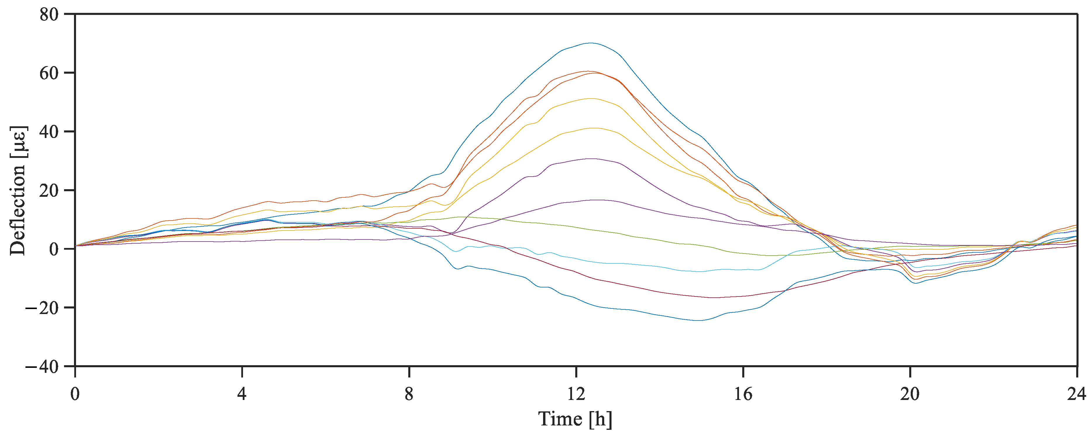
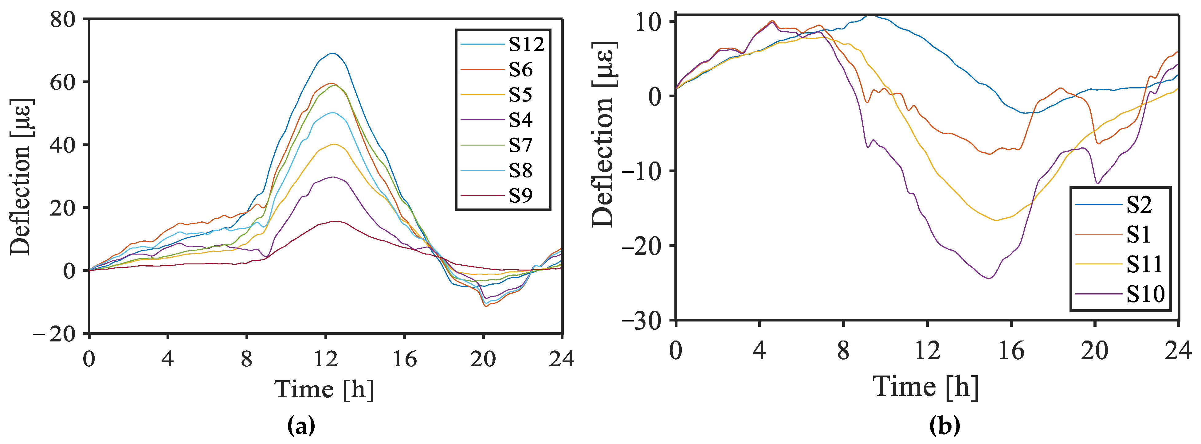
3.1. Bridge Introduction

As shown in Figure 3, the engineering project used in this study is a cable-stayed bridge with a main span of 456 m and total length of 1150 m. The numbers and locations of the vertical deflection sensors are shown in Figure 4. S denotes sensor.

The SHM system of the bridge collected monitoring data at a sampling frequency of 10 Hz. The data were resampled at 10 s intervals to obtain static temperature-induced deflection data. Figure 5 shows the recorded static temperature-induced deflection from the 11 sensors in a day. These monitoring data can be organized in a matrix format. There were significant differences among the data from the sensors at different locations. The relative torsion between different sections leads to different correlations of temperature-induced deflection in these sections [18]. To ensure the effect of missing recovery, the data with strong correlations were aggregated into a single cluster. Data from sensors placed in the main span were aggregated into one cluster, and data from sensors placed in the side spans were aggregated into another cluster. The clustering results for the deflection data are shown in Figure 6. For ease of description, the main span sensor data cluster is referred to as Cluster 1 and the side span sensor data cluster is referred to as Cluster 2.

We developed a framework for missing-data recovery based on Bayesian matrix factorization, as shown in Figure 7. We followed this framework to perform validation experiments, as detailed in Section 4.

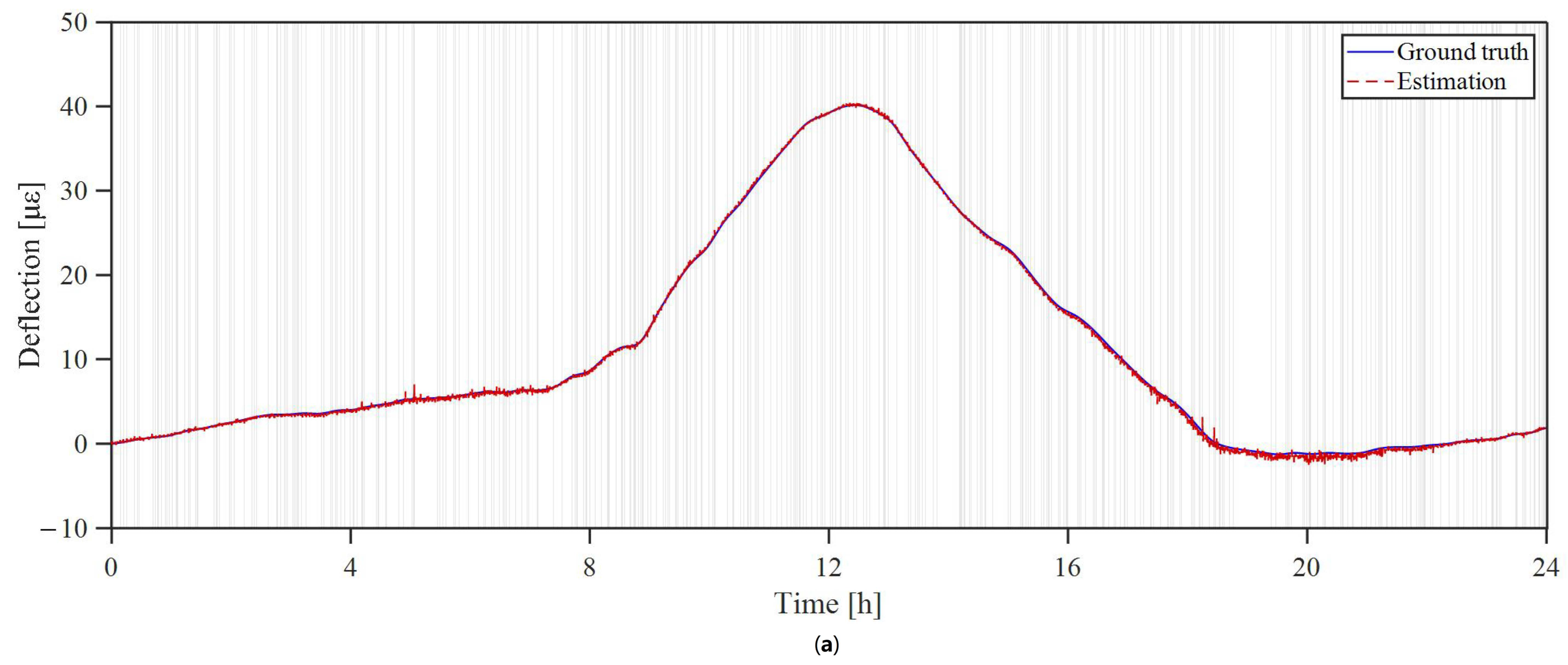
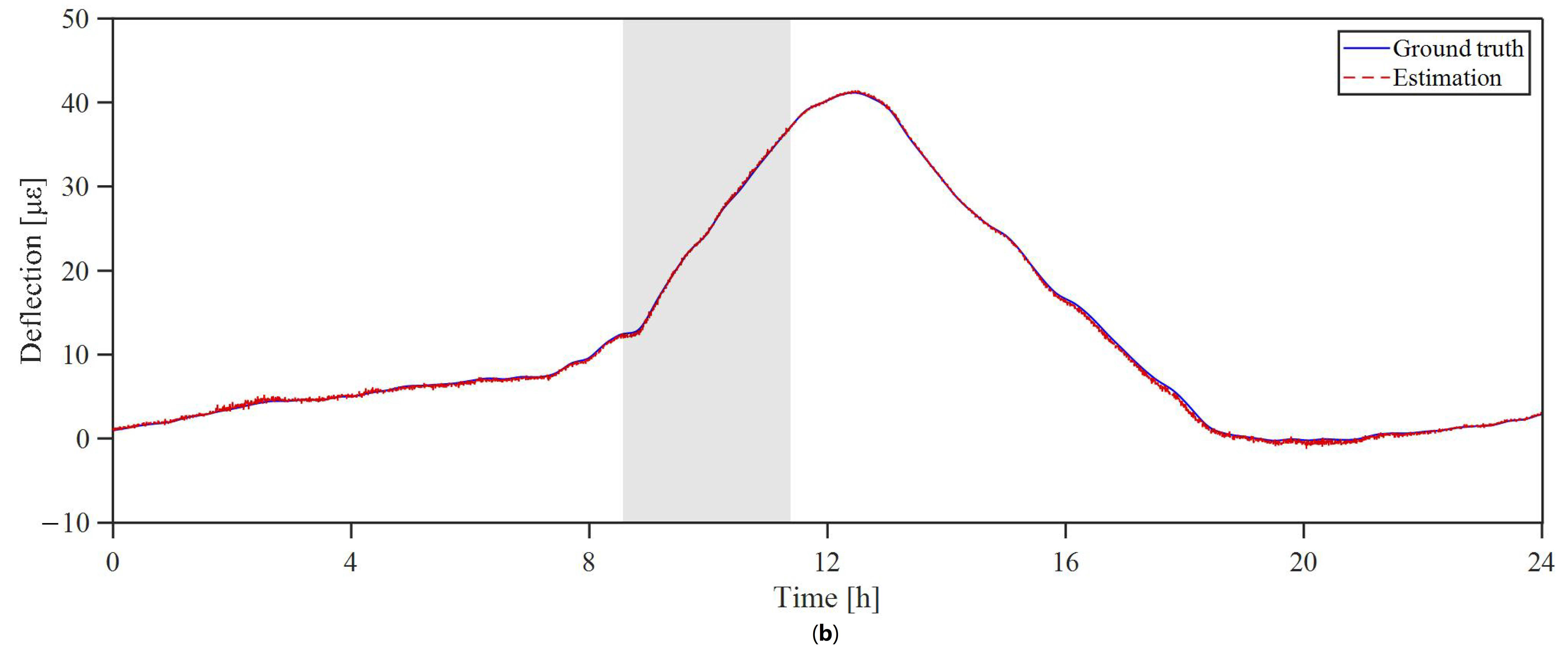
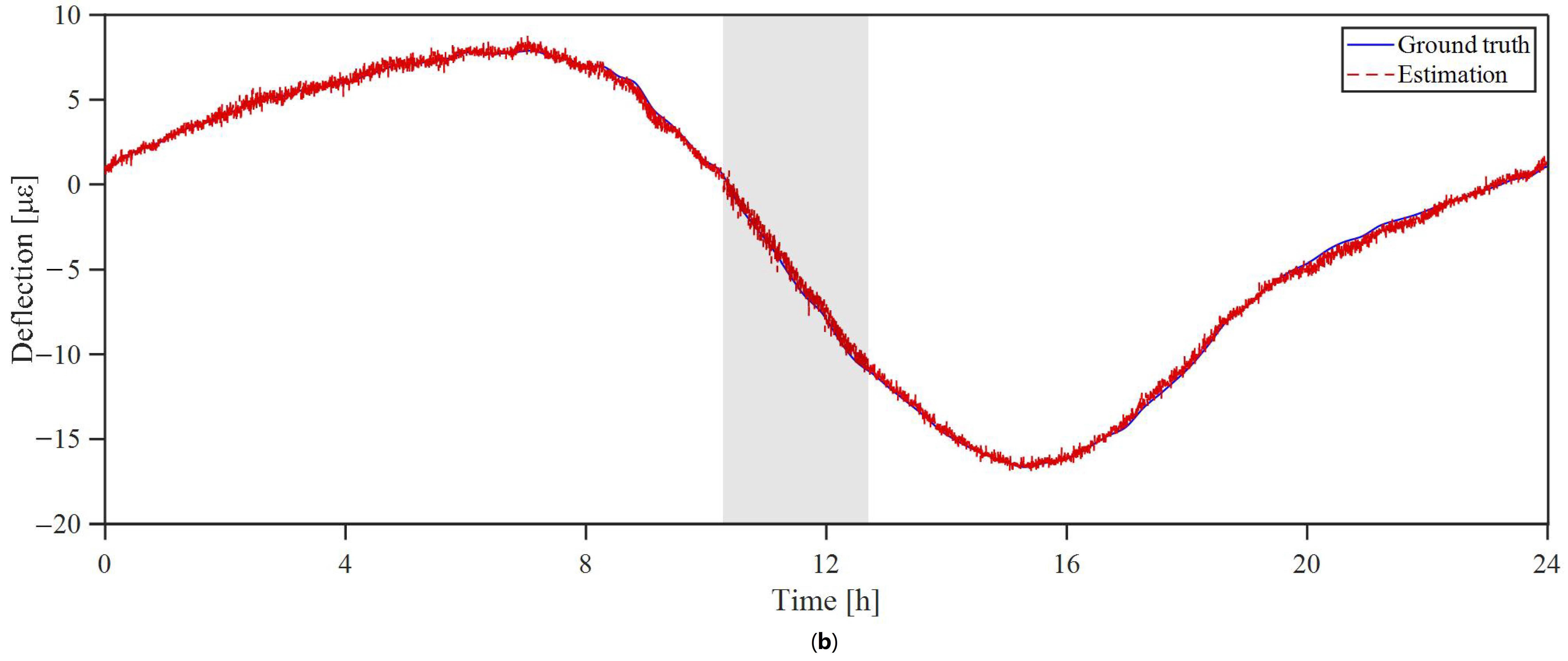
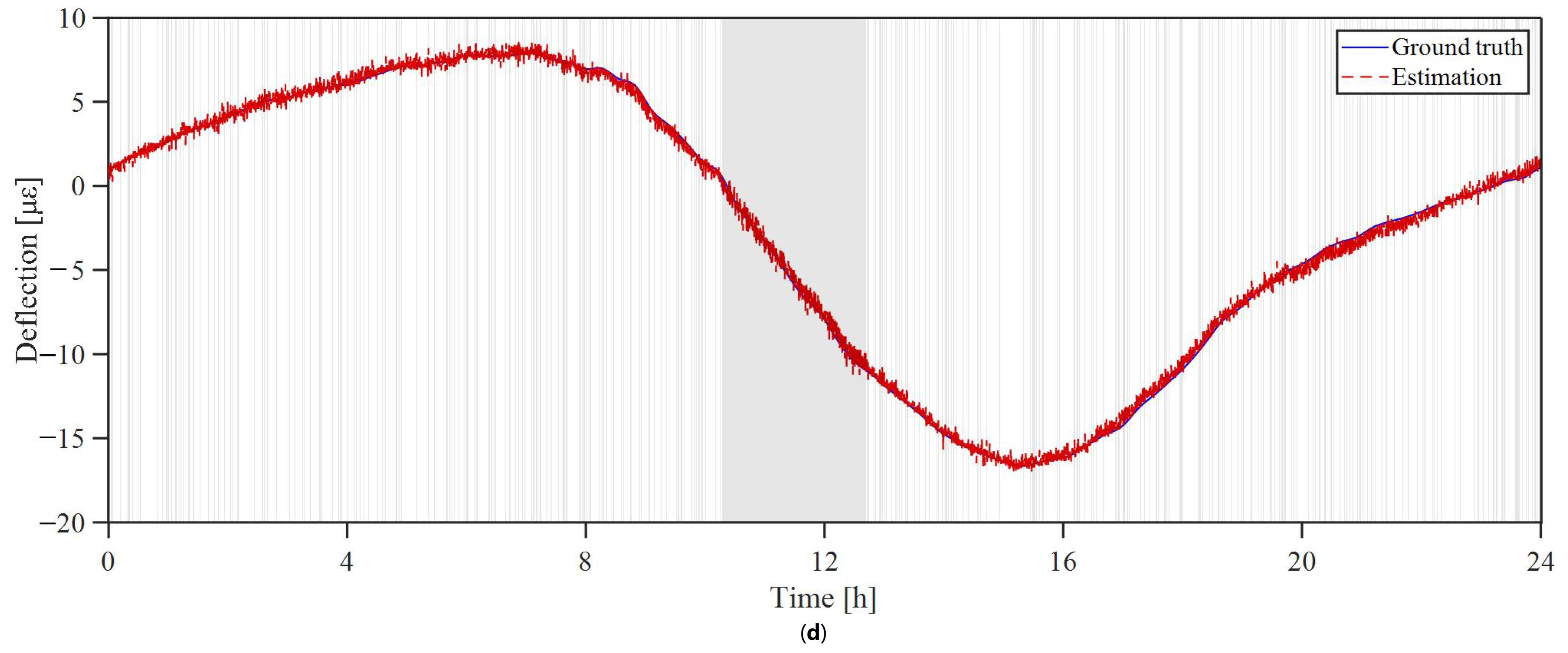
3.2. Missing-Data Recovery Result

To demonstrate the performance of the proposed method, the type of missing data should first be defined. The missing rate, which is the ratio of the number of missing data to the total number of observations, is introduced in the missing setting. Second, to simulate the missing scenarios in real monitoring data, three basic missing scenarios were defined for the data in a matrix form [19]. The first scenario is referred to as random missing (RM), which is random-missing data in the matrix. The elements in the matrix were randomly set as missing. The next scenario is called structured missing (SM), that is, there is continuous-missing data (i.e., 1 h or 1 d) owing to sensor failure during certain periods. Although this is the most common missing scenario in practical applications, it is more challenging and less studied in the literature. We simulated an actual missing condition by randomly selecting a continuous monitoring period and deleting the data to structurally remove the deflection data. The final scenario is called mixing missing (MM), which consists of random missing and structured missing proportions. In the following experiments, the scalars are initialized as: ${\mathrm{a}}_0={10}^{-6}$,${\mathrm{b}}_0={10}^{-6}$,${\mathrm{c}}_0={10}^{-6}$, and ${\mathrm{h}}_0={10}^{-6}$. Vector λ is initialized as a unit vector.

We set up four missing cases: 10% RM, 10% SM, 20% SM, and 20% MM, as shown in

Table 1. Cases with large-proportion structures missing.

Case	${\mathit{\eta }}_{\mathit{m}}$	Missing Type
1	10%	RM
2	10%	SM
3	20%	SM
4	10%SM + 10%RM	MM

. We defined a sparse binary matrix to facilitate the location of missing data and compared the recovery results with the ground truth. The recovery accuracy is defined as the mean absolute error (MAE) between the estimations and the corresponding ground truth normalized by the absolute mean of the target value:

$${\rho }_r=\left(1-\frac{\frac{1}{n}{{\displaystyle \sum }}_{i=1}^n\left|y_i-y_i^{*}\right|}{\frac{1}{n}{{\displaystyle \sum }}_{i=1}^n\left|y_i\right|}\right)\times 100\%,$$

(19)

where $y_i^{*}$ and $y_i$ represent the estimation and ground truth at position i, respectively.

In Equation (19), $\frac{1}{n}{\displaystyle \sum }_{i=1}^n\left|y_i-y_i^{*}\right|$ is the average of the sum of the errors between all estimations and ground truth. However, this does not truly reflect the missing-data recovery accuracy of BMF because the accuracy is also related to the value of ground truth. Therefore, the recovery accuracy is defined as the mean absolute error (MAE) between the estimations and the corresponding ground truth normalized by the absolute mean of the target value.

Data from sensor S5 were used to present the results of Cluster 1. The missing recovery results for Cluster 1 are shown in Figure 8. The data from sensor S10 were used to present the results of Cluster 2. The results of Cluster 2 are shown in Figure 9. The gray areas indicate missing data. The accuracy of the recovery results for the two clusters is shown in Figure 10a,b, respectively.

It is clear that the estimations match well with the ground truth in all cases, which demonstrates the good missing recovery performance of the proposed method. As can be seen from Figure 10, the missing recovery accuracy of Cluster 1 is higher than that of Cluster 2 in the same missing case. This can be seen more visually in Figure 9. Compared to the results of Cluster 1, the results of Cluster 2 have more dramatic fluctuations around the actual value. This is owing to the poorer linear correlation among deflections of side spans and the smaller amount of data. Nevertheless, the degree of fluctuation was still within acceptable limits, and the baseline still matched well with the ground truth. In addition, it can be found from Figure 10 that the trend of missing recovery accuracy of all missing cases of Cluster 1 are the same as that of Cluster 2. Specifically, the missing recovery accuracy of class 1 and class 2 is the lowest in case 3, compared to other cases. This is because recovering structured missing is more challenging than recovering random missing, which is also illustrated by the lower missing recovery accuracy of case 2 than that of case 1 for both Cluster 1 and Cluster 2. In conclusion, Bayesian matrix factorization can achieve good results for monitoring data at different locations and different missing types.

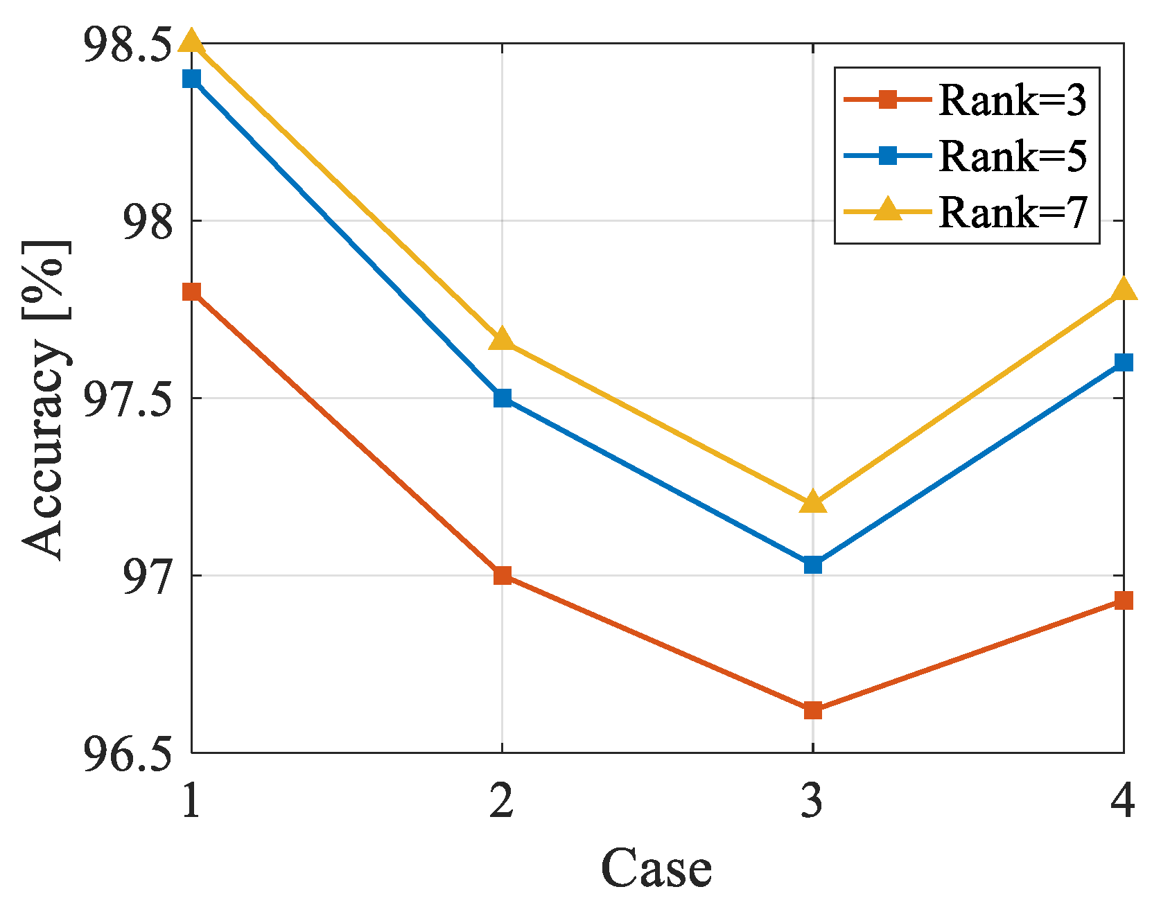
3.3. Analysis of Rank

Many studies have focused on investigating the effects of missing data on tensor representation. It was found in [20] that the correlation across time and modalities presented in high-quality data is broken by missing data and noise, which results in the need to represent the matrix with a higher rank. This study also investigated the effect of missing data on the preset rank of the matrix. We compared the missing-data recovery performance of Bayesian matrix factorization with different preset ranks under the same cases in Table 1 using data from Cluster 1. The results are summarized in Figure 11.

As shown in Figure 11, the proposed method shows a better performance in all cases when the rank increases. The missing-data recovery accuracy at rank = 5 is significantly higher than that at rank = 3, whereas the missing-data recovery accuracy at rank = 7 is only moderately better than that at rank = 5. This shows that Bayesian matrix factorization still has a good performance for missing-data recovery when the rank is smaller, even if the correlation of the dataset is broken by missing data. In summary, because a larger rank increases the computational burden but does not significantly improve the accuracy of missing-data recovery, a smaller rank is recommended in practice.

3.4. Comparison with Support Vector Machine

Support vector machine (SVM) as a classification algorithm can effectively avoid the curse of dimensionality. It shows many unique advantages in solving small sample and nonlinear problems and can be extended to classification, regression, and time series prediction [21]. To illustrate the advantage of Bayesian matrix factorization (BMF), we compare the performance of BMF and SVM in missing-data recovery. The radial basis function is chosen as the classification kernel function of SVM. The parameters of SVM directly affect the performance of SVM. Therefore, to improve the prediction performance of the model, the grid search (GS) method is introduced to find the optimal parameters. To avoid overfitting and underfitting, the cross-validation method is used to perform a parameter search with the minimum root mean square error of the training set as the fitness function.

The dataset considered in this section is Cluster 1, used in Section 3.3. The comparison experiments include two cases: (1) 10% SM and (2) 20% SM. Specifically, 10% SM or 20% SM is set in monitoring data from only one sensor for each experiment. The non-missing data from this sensor and data from the other eight sensors are used as inputs of BMF and SVM to recover missing data. Then the results of BMF and SVM can be compared. The compared results are shown in Figure 12.

As shown in Figure 12, the recovery accuracy of BMF is higher than that of SVM for the same case, indicating that the proposed model is better than SVM. Furthermore, the accuracy of recovering missing data from different sensors by SVM fluctuates greatly for the same missing rate. The missing recovery accuracy of SVM decreases significantly as the missing rate increases. In contrast, BMF achieves high and stable missing recovery accuracy in different cases, which shows that BMF is more robust than SVM.

3.5. Comparison with K-Nearest Neighbor

K-Nearest Neighbor (KNN) is a classification and regression algorithm [22]. When a new sample is input into the model, the KNN algorithm finds K samples that are closest to this sample in training set. Then this new sample is assigned to the class to which the majority of these K samples belong.

For the problem of restoring missing data, the KNN algorithm finds the K nearest “neighbors” of the sample that has missing attributes, and then the average of the corresponding attributes of these “neighbors” is used as the restored value of the missing attributes of the sample. In this way, missing data can be restored using the spatio-temporal correlation between monitoring data.

As shown in Figure 13, monitoring data measured by all sensors at the same moment are one sample, and the data point measured by a sensor at that moment is an attribute value of that sample. If monitoring data collected by sensor S2 of a sample are missing, KNN will use the monitoring data measured by other sensors to calculate the distance between this missing sample and other un-missing samples to find the K samples that are closest to this missing sample. The distance calculation formula is as follows:

$${\mathrm{d}}_{\mathrm{j}}=\sqrt{\frac{\mathrm{N}}{{\mathrm{n}}_{\mathrm{j}}}\times {\displaystyle \sum }_{\mathrm{i}=1}^{{\mathrm{n}}_{\mathrm{j}}}{\left({\mathrm{x}}_{\mathrm{i},\mathrm{j}}-{\mathrm{x}}_{\mathrm{i},0}\right)}^2},$$

(20)

where $d_j$ denotes the distance of the jth sample from the missing sample; N denotes the total number of attributes; $n_j$ denotes the number of attributes available for calculating $d_j$; $x_{i,j}$ denotes the ith attribute value used to calculate $d_j$ in the jth sample; and $x_{i,0}$ denotes the ith attribute value in the missing sample used to calculate $d_j$.

The dataset considered in this section is Cluster 1, used in Section 3.3. The cases of comparison experiment are the same as those in Section 3. 4. The compared results are shown in Figure 14.

As shown in Figure 14, the recovery accuracy of BMF is higher than that of KNN for the same case, indicating that the proposed model is better than KNN. As with SVM, missing-data recovery accuracy of KNN is very unstable and much lower than that of BMF. This illustrates that BMF can better extract the spatio-temporal correlation between data to restore missing data.

4. Discussion

In this study, we applied Bayesian matrix factorization to the recovery of missing monitoring data and verified the good performance of the proposed method with monitoring data of an in-service bridge. The experimental results show that Bayesian matrix factorization can well recover different types of missing monitoring data from different bridge locations, which demonstrates the great potential of Bayesian matrix factorization for application in structural health monitoring.

Compared with previous studies, this study better considers the difficulties of applying an algorithm to practical engineering, including the difficulty of obtaining high-quality datasets and the tuning. In addition, Bayesian matrix factorization can extract the spatio-temporal dependence among monitoring data to recover the missing data from all sensors simultaneously.

However, there is limitation in this study. In practical engineering, there are other types of data anomalies in monitoring data besides missing data, such as outlier, baseline-shift, and noise, which may interfere with the results of missing recovery. This is an important factor that limits the application of Bayesian matrix factorization. We can reduce the impact of data anomalies on the missing recovery by improving the robustness of the model.

5. Conclusions

A Bayesian matrix factorization model for missing health-monitoring data recovery was presented in this study. In the validation experiments, a random missing scenario and a missing structure were both introduced while considering different proportions of missing data. Accurate recovery results indicate that the proposed model can recover an incomplete SHM data matrix with good accuracy.

This study has demonstrated that matrix factorization is an effective solution to the missing-data problem, and can be a highly beneficial tool for addressing key issues in SHM. Future research directions and outlooks are presented in this paper. The possible future research directions are as follows. First, the proposed model can be extended as a model that can select the rank automatically; second, we can develop an incremental framework based on Bayesian matrix factorization to recover missing data in real time.

References

- Sun, L.; Shang, Z.; Xia, Y.; Bhowmick, S.; Nagarajaiah, S. Review of Bridge Structural Health Monitoring Aided by Big Data and Artificial Intelligence: From Condition Assessment to Damage Detection. Eng. Struct. 2020, 146, 04020073. [Google Scholar] [CrossRef]
- Jiang, H.; Wan, C.; Yang, K.; Ding, Y.; Xue, S. Continuous Missing Data Imputation with Incomplete Dataset by Generative Adversarial Networks-Based Unsupervised Learning for Long-Term Bridge Health Monitoring. Struct. Health Monit. Int. J. 2021, 21, 14759217211021942. [Google Scholar] [CrossRef]
- Marcantonio, V.; Monarca, D.; Colantoni, A.; Cecchini, M. Ultrasonic waves for materials evaluation in fatigue, thermal and corrosion damage: A review Mechanical. Syst. Signal Process. 2019, 120, 32–42. [Google Scholar] [CrossRef]
- Jeong, S.; Ferguson, M.; Hou, R.; Lynch, J.; Sohn, H.; Law, K.H. Sensor Data Reconstruction Using Bidirectional Recurrent Neural Network with Application to Bridge Monitoring. Adv. Eng. Inform. 2019, 42, 100991. [Google Scholar] [CrossRef]
- Liu, H.; Ding, Y.; Zhao, H.; Wang, M.; Geng, F.F. Deep Learning-Based Recovery Method for Missing Structural Temperature Data Using LSTM Network. Struct. Monit. Maint. 2020, 7, 109–124. [Google Scholar]
- Rautela, M.; Gopalakrishnan, S. Ultrasonic guided wave based structural damage detection and localization using model assisted convolutional and recurrent neural networks. Expert Syst. Appl. 2020, 167, 114189. [Google Scholar] [CrossRef]
- Wan, H.-P.; Ni, Y.-Q. Bayesian multi-task learning methodology for reconstruction of structural health monitoring data. Struct. Health Monit. 2018, 18, 1282–1309. [Google Scholar] [CrossRef]
- Chen, Z.; Li, H.; Bao, Y. Analyzing and modeling inter-sensor relationships for strain monitoring data and missing data imputation: A copula and functional data-analytic approach. Struct. Health Monit. 2018, 18, 1168–1188. [Google Scholar] [CrossRef]
- Rabcan, J.; Levashenko, V.; Zaitseva, E.; Kvassay, M.; Subbotin, S. Non-destructive diagnostic of aircraft engine blades by Fuzzy Decision Tree. Eng. Struct. 2019, 197, 109396. [Google Scholar] [CrossRef]
- Ji, Y.; Wang, Q.; Li, X.; Liu, J. A Survey on Tensor Techniques and Applications in Machine Learning. IEEE Access 2019, 7, 162950–162990. [Google Scholar] [CrossRef]
- Nie, X.; Yin, Y.; Sun, J.; Liu, J.; Cui, C. Comprehensive Feature-Based Robust Video Fingerprinting Using Tensor Model. IEEE Trans. Multimed. 2016, 19, 785–796. [Google Scholar] [CrossRef]
- Hu, W.R.; Tao, D.; Zhang, W.; Xie, Y.; Yang, Y.H. The Twist Tensor Nuclear Norm for Video Completion. Ieee Trans. Neural Netw. Learn. Syst. 2017, 28, 2961–2973. [Google Scholar] [CrossRef] [PubMed]
- Xie, K.; Wang, L.; Wang, X.; Xie, G.; Wen, J.; Zhang, G.; Cao, J.; Zhang, D. Accurate Recovery of Internet Traffic Data: A Sequential Tensor Completion Approach. IEEE/ACM Trans. Netw. 2018, 26, 793–806. [Google Scholar] [CrossRef]
- Zheng, C.; E, H.; Song, M.; Song, J. CMPTF: Contextual Modeling Probabilistic Tensor Factorization for recommender systems. Neurocomputing 2016, 205, 141–151. [Google Scholar] [CrossRef]
- Ren, P.; Chen, X.; Sun, L.; Sun, H. Incremental Bayesian matrix/tensor learning for structural monitoring data imputation and response forecasting. Mech. Syst. Signal Process. 2021, 158, 107734. [Google Scholar] [CrossRef]
- Salehi, H.; Burgueño, R. Emerging artificial intelligence methods in structural engineering. Eng. Struct. 2018, 171, 170–189. [Google Scholar] [CrossRef]
- Bahadori, M.T.; Yu, Q.; Liu, Y. Fast Multivariate Spatiotemporal Analysis via Low Rank Tensor Learning. In Proceedings of the 28th Conference on Neural Information Processing Systems (NIPS), Montreal, Canada, 8–13 December 2014; Volume 27. [Google Scholar]
- Yue, Z.-X.; Ding, Y.-L.; Zhao, H.-W. Deep Learning-Based Minute-Scale Digital Prediction Model of Temperature-Induced Deflection of a Cable-Stayed Bridge: Case Study. J. Bridg. Eng. 2021, 26, 05021004. [Google Scholar] [CrossRef]
- Chen, X.; He, Z.; Wang, J. Spatial-temporal traffic speed patterns discovery and incomplete data recovery via SVD-combined tensor decomposition. Transp. Res. Part C Emerg. Technol. 2018, 86, 59–77. [Google Scholar] [CrossRef]
- Liang, P.P.; Liu, Z.; Tsai, Y.-H.H.; Zhao, Q.; Salakhutdinov, R.; Morency, L.-P. Learning Representations from Imperfect Time Series Data via Tensor Rank Regularization. In Proceedings of the 57th Annual Meeting of the Association-for-Computational-Linguistics (ACL), Florence, Italy, 28 July–2 August 2019; pp. 1569–1576. [Google Scholar]
- Sun, J.; Zhang, J.; Gu, Y.; Huang, Y.; Sun, Y.; Ma, G. Prediction of permeability and unconfined compressive strength of pervious concrete using evolved support vector regression. Constr. Build. Mater. 2019, 207, 440–449. [Google Scholar] [CrossRef]
- Peterson, L.E. K-nearest neighbor. Scholarpedia 2009, 4, 1883. [Google Scholar] [CrossRef]