Methodology to Estimate the Impact of the DC to AC Power Ratio, Azimuth, and Slope on Clipping Losses of Solar Photovoltaic Inverters: Application to a PV System Located in Valencia Spain

Abstract

Renewable power capacity sets records annually, driven by solar photovoltaic power, which accounts for more than half of all renewable power expansion in 2021. In this sense, photovoltaic system design must be correctly defined before system installation to generate the maximum quantity of energy at the lowest possible cost. The proposed study analyses the oversizing of the solar array vs. the capacity of the solar inverter, seeking low clipping losses in the inverter. A real 4.2 kWp residential PV installation was modelled and validated using the software SAM and input data from different sources, such as a weather station for weather conditions, ESIOS for electricity rates, and FusionSolar to obtain energy data from the PV installation. Once data were validated through SAM, the DC to AC ratio was varied between 0.9 and 2.1. The azimuth and slope sensitivity analyses were performed regarding clipping inverter losses. Results have been evaluated through the energy generated and the discounted payback period, showing that, depending on the weather conditions, slope, and azimuth, among others, it is advisable to increase the DC to AC ratio to values between 1.63 and 1.87, implying low discounted payback periods of about 8 to 9 years. In addition, it was observed that inverter clipping losses significantly vary depending on the defined azimuth and slope.

1. Introduction

Solar photovoltaic (PV) generation increased by a record 179 TWh (up 22%) in 2021 to exceed 1000 TWh [1], reaching the second-highest absolute growth in energy generation of all renewable technologies after wind, becoming, as well, the lowest-cost option for new electricity generation. Nevertheless, to meet the Net-Zero Emissions by 2050 Scenario, there must be an average annual generation growth, requiring better design of PV installations and policy regulations, especially in emerging and developing countries. Consequently, the compromises between the form and function of PV generator sizing on buildings are an essential aspect that architects and building planners must address as PV becomes a more mainstream electricity generation alternative worldwide. Designers of PV systems do not have guidelines for the optimal sizing of inverters in their projects regarding the DC to AC ratio and the influence of the slope and azimuth of the PV system in inverter losses. Designers disagree on which parameter must be the priority [2], depending on the installation location, the available PV panel capacity, the reactive power profile, etc. This is a major problem since optimising the installation characteristics of PV systems guarantees a greater generation of electric energy and less economic costs.

Focusing on PV systems’ design, prior researchers have studied the factors which lead to an optimum design of grid-connected inverter sizing, taking into account the effect of different factors: meteorological [3], economic [4], and inverter characteristics. Refs. [5,6] use the return on investment as a parameter to show that the optimum inverter size may notably vary by location and context. These studies can be considered as a preliminary step before focusing on optimising the DC to AC ratio and delving into the influence of specific installation parameters, such as the slope and the azimuth.

In the next stage, in [7] the authors address the influence of the DC input voltage on DC/AC conversion efficiency, considering the technical characteristics of the inverter and PV modules, the climatic characteristics of the site, and the orientation and tilt of the PV generator. However, they slightly delve into a recommendation of the array-to-inverter power sizing ratio, the DC to AC ratio. They give a brief recommendation that for the sizing of PV systems in low-latitude semi-desert climates, the DC to AC ratio should be 1.05 for c-Si and 0.95 for CdTe.

On the other hand, the effect of weather conditions different from the usual ones in solar inverters has been studied in [8], particularly the over-irradiance on PV systems with different inverter sizing factors. The over-irradiation events show an increase in the electric current of the PV generator, which can affect the operation of the protection devices and even cause damage to the DC/AC inverters. This research shows that PV systems located in very high-irradiance places with undersized inverters may lose electricity generation, in addition to reducing their useful life due to the stress of the components due to overtemperature, resulting in inverter changes over the life of the PV system. Therefore, the DC to AC ratios must be carefully calculated so as not to affect the inverter’s performance.

Traditional studies have used weather forecasts to estimate the power profile of PV systems [9]. However, other investigations have shown that a PV plant’s forecast errors depend not only on the variability of the weather conditions but also on its design parameters [10].

The impact of several PV plant design parameters, the slope angle and DC to AC ratio, among others, on the error of the irradiance-to-power conversion (the accuracy of PV power forecasts) has been studied in [11]. Their results reveal that the design parameters highly influence the PV power forecast errors. They concluded that a slope angle of 45° increases the error metrics up to 49% compared to a horizontal plane, and under-sizing the inverters by a 1.5 sizing factor leads to an average error decrease of up to 25%, while the effect of the row spacing is less than 5% in most cases. However, their final recommendations regarding the optimal PV design are not that simple. They state that it can only be performed by using detailed techno-economic modelling, a more elaborated way of calculating the monetary value of power forecasts, and accounting for the time dependence of the costs and penalties.

Meanwhile, the DC to AC ratio optimisation for large-scale grid-connected solar photovoltaic installations has been studied in [12], where the authors investigated Brazil’s Northeast Region’s solar potential to improve the design of system components, such as the inverter. A methodology to estimate the optimal inverter loading ratio employing one year of solar generation data, analysing five different technologies of PV panels, was developed. The authors stated that the standard inverter loading ratio on utility-scale PV plants in Brazil implies overload losses of between 0.3% and 2.4%, depending on the technology used. Indeed, the results show that the optimal inverter loading ratio for crystalline Si PV technology in that area should be 126%. Additionally, the authors of [2] have studied the DC to AC ratio, but in this case from the reactive power point of view, as they propose to evaluate the system-level reliability of a single-phase two-stage PV inverter performing reactive power compensation from three different mission profiles under different inverter sizing ratios. The results showed that over-sizing the PV inverter can increase the generated energy, negatively impacting the system lifetime, independent of the region and reliability. It increases system costs due to more inverter replacements, affecting the LCOE.

Additionally, Ref. [13] aims to undersize the inverter of residential PV systems to decrease investment costs to then decrease solar PV electricity production costs. The authors state that they obtained higher optimal DC to AC ratios than in central Europe, possibly due to the northern Finland location. It allows more significant under-sizing as less energy is clipped even at higher DC to AC ratios of 1.6, 1.8, and 2.08 (in the case of 30° slope south-oriented arrays). Results of this work show that the smaller the system is, the more the inverter should be undersized, which is explained by the cost distribution of the solar PV systems; in smaller systems, the proportion of the inverter in the investment is more significant, while in more extensive systems the array prices are the main factor in the total investment. Additionally, the study shows that the optimal array DC to AC ratio for the southwest–southeast facade systems is 1.8, 1.9, and 2.17 for the inverters under investigation.

Furthermore, regarding the study of the slope and azimuth, Ref. [14] tries to define the ideal position of PV modules in buildings to receive great relative radiation levels in Brazilian sites, spanning latitudes from 0° to 30°. The authors state that variations in azimuth or slope did not cause large annual irradiation losses in up to around 20° slope angles and in latitudes up to 10°. Conversely, large slopes (especially vertical walls) result in significant annual solar irradiation losses irrespective of azimuthal deviation, and zero azimuth deviation (north orientation) is not required at those latitudes. Regarding the azimuth, they state that the east or west orientation is even better than the north orientation for vertical walls at low latitude sites, leading to 5–10% energy gains over the year. However, as the study is subject to the installation site, it can hardly be applied to other regions. According to [15], the analyses can be extended to other types of technologies. A concentrator photovoltaic power plant model is developed taking into consideration different characteristics, such as different inverter schemes, efficiencies, capacities, DC to AC ratios, etc., to obtain the optimum inverter solution for these types of installations, ranging DC to AC ratios from 1.01 to 1.67 for maximum performance ratio, and from 1.53 to 1.79 for minimum levelized cost of energy. Likewise, authors in [16] calculate an optimum size of a grid-connected inverter in high-concentrator photovoltaic systems, being aware that the DC to AC ratio calculated depends on the climatic characteristics of the site (irradiance, temperature, height above sea level, etc.). Their results show that in high-concentrator photovoltaic systems, the inverter can be sized between 84% and 112% of the rated capacity of the system generator at Concentrator Standard Test Conditions depending on the scenario considered for maximising the final energy yield of the system.

Finally, it must be considered that the correct design of the installation parameters (slope and azimuth of the PV panels and inverter DC to AC ratio) is a key factor in reducing the cost of PV systems [17]. Additionally, as inverters’ penetration levels in the grid rise, complying at all times with their input current and voltage plays an essential role in ensuring they operate at maximum efficiency.

The manuscript is organised as follows: Section 2 provides information about the method used to model the system, Section 3 shows the validation of data and results, Section 4 deals with the discussion of results, and finally, Section 5 summarises the conclusions of this work.

2. Methods

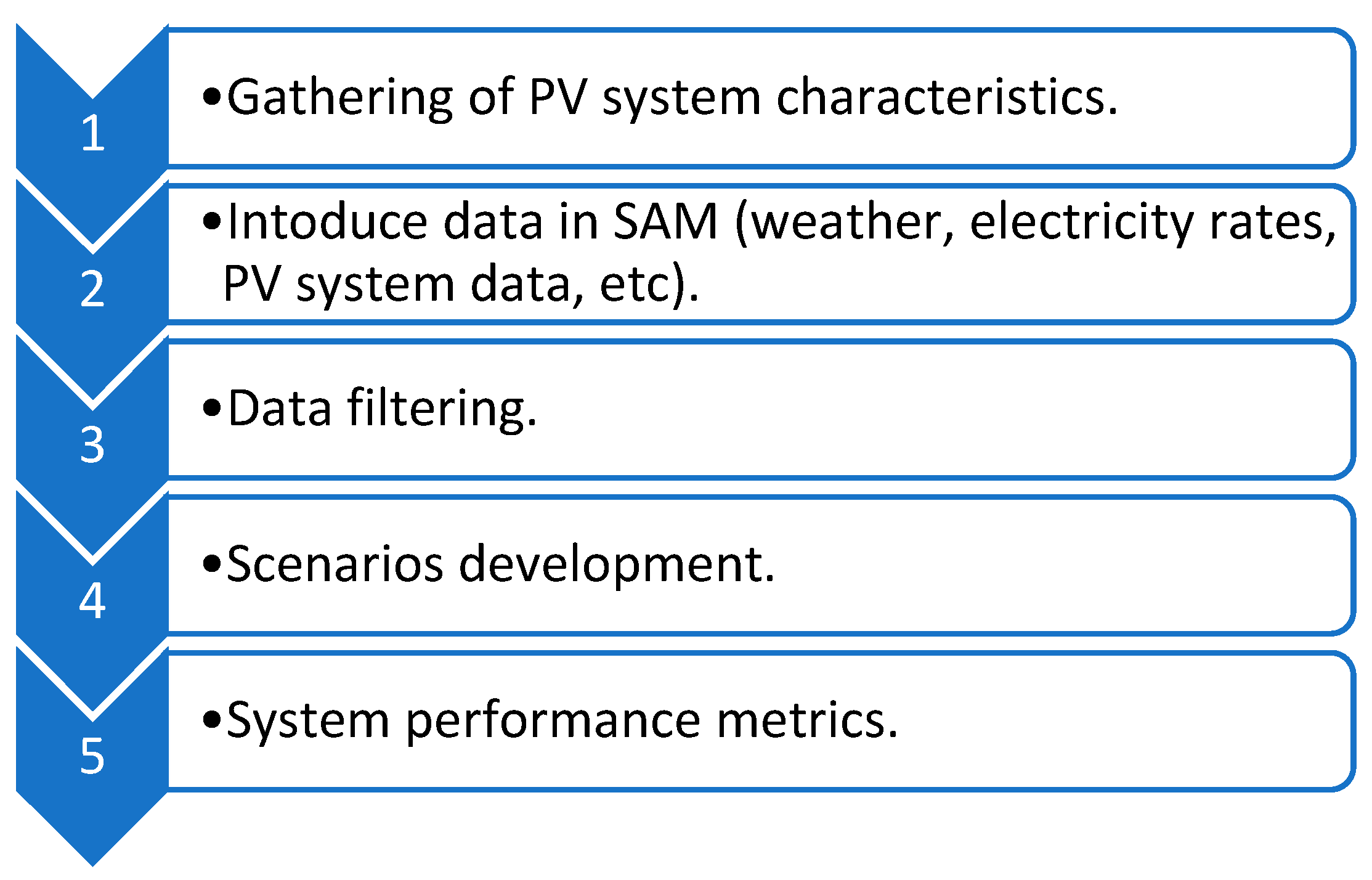
A residential PV solar generation site in Valencia, Spain, has been modelled to study the impact of the DC to AC ratio on PV generation profiles. Several simulations were performed in NREL System Advisor Model (SAM) software, version 2020.2.29, from the National Renewable Energy Laboratory (NREL). Total energy production and clipping energy results were obtained. Decision-making has been guided by considering the characteristics of the real residential PV system for a rooftop installation. The subsections below explain the main aspects of the PV system, the methodology used to obtain the input data for the SAM software, data filtering, modelling of the generation system, scenarios proposed, and system performance metrics (Figure 1). Additionally, further subsections explain the PV performance model used in SAM.

2.1. PV System Characteristics

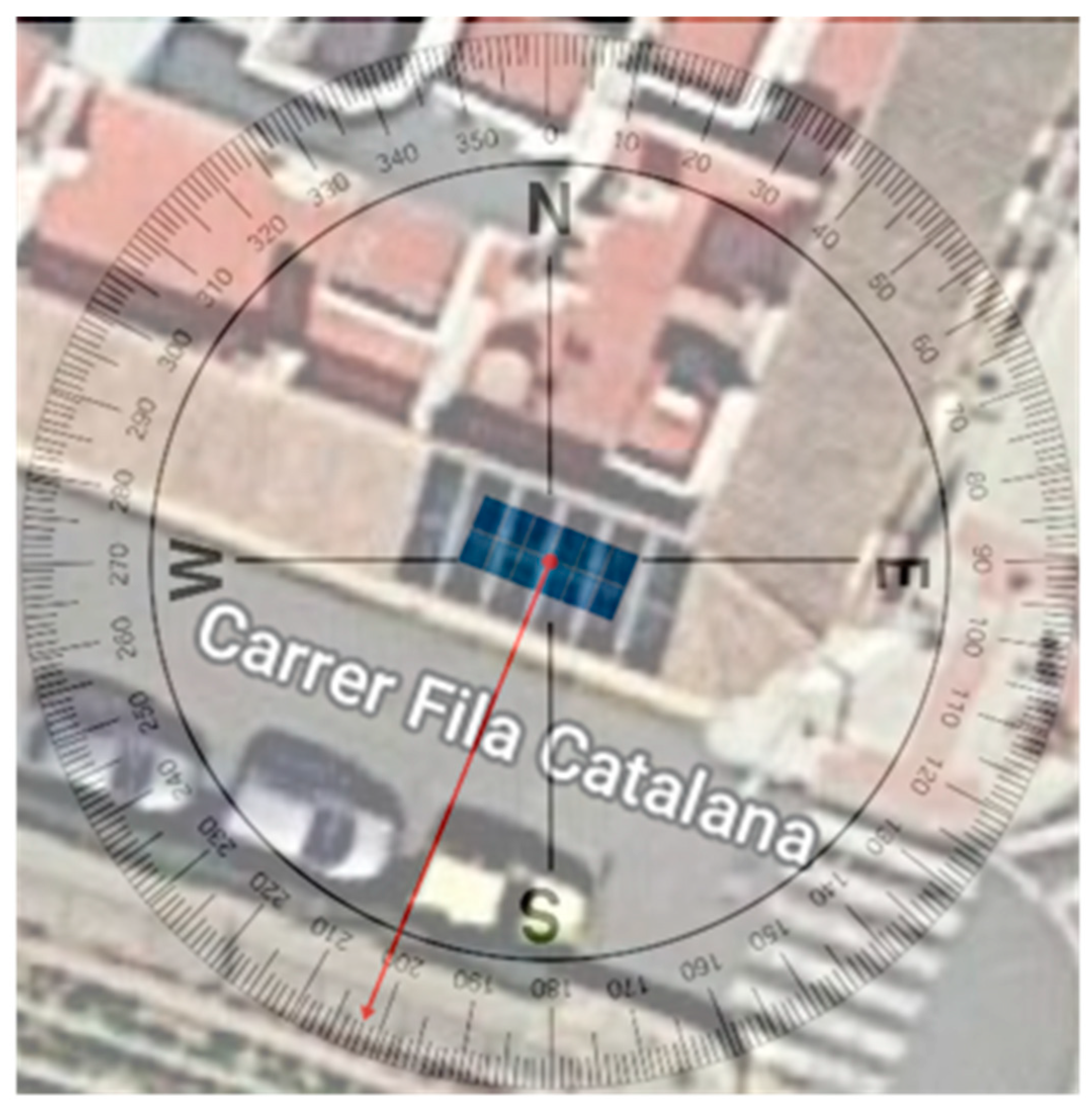
The real PV system analysed is located in a town in the Valencian region and was commissioned in 2020. The 4.2 kWp PV system comprises twelve 350 Wp rooftop panels installed with an azimuth of 202° and a slope of 20.5°. The PV system is divided into two strings of six panels. Each string is connected to an MPPT inverter input.

Table 1. PV panel characteristics.

PV Panel	Hyundai HiES350SG
Cell type	Mono-Crystalline Silicon
Nominal output (W)	350
Module area (m2)	1.7323
Nominal operating cell temperature (°C)	42.3
Maximum power point voltage (V)	37.6
Maximum power point current (A)	9.31
Open-circuit voltage (V)	45.4
Short-circuit current (A)	9.6
Temperature coefficient of Voc (%/°C)	−0.27
Temperature coefficient of Isc (%/°C)	0.04
Temperature coefficient of max. power point (%/°C)	−0.34

shows the electrical characteristics of the PV panels installed, at Standard Test Conditions (STC), with a 20-year product warranty, PERC Shingled and Anti-LID/PID technology, during their lifetime.

Table 2. Solar inverter characteristics.

Solar Inverter	Huawei SUN2000 3KTL
Maximum AC output power (Wac)	3000
Weighted efficiency (%)	97.6
Nominal AC voltage (Vac)	230
Maximum DC voltage (Vdc)	600
Maximum DC current (Adc)	11
Minimum MPPT DC voltage (Vdc)	90
Nominal DC voltage (Vdc)	380
Maximum MPPT DC voltage (Vdc)	500
Number of MPPT inputs	2

shows the electrical characteristics of the solar inverter installed, for a 3 kW inverter, a model prepared for the integration at self-consumption systems, two MPPTs with a wide work range, and a 5-year product warranty. The inverter has a metering system to measure the solar PV parameter of the array and at the inverter output. In addition, another power meter measures the parameters of the energy imported and exported from the utility grid. Additionally, through an energy balance, energy demand is obtained. The data-saving resolution is five minutes.

It must be noted that the azimuth value is specified in the paper according to the way it has to be expressed in SAM, as shown in Figure 2, where the north orientation is considered 0°, 90° E, 180° S, and west 270° W.

2.2. SAM Input Data

2.2.1. Weather Data for Simulations

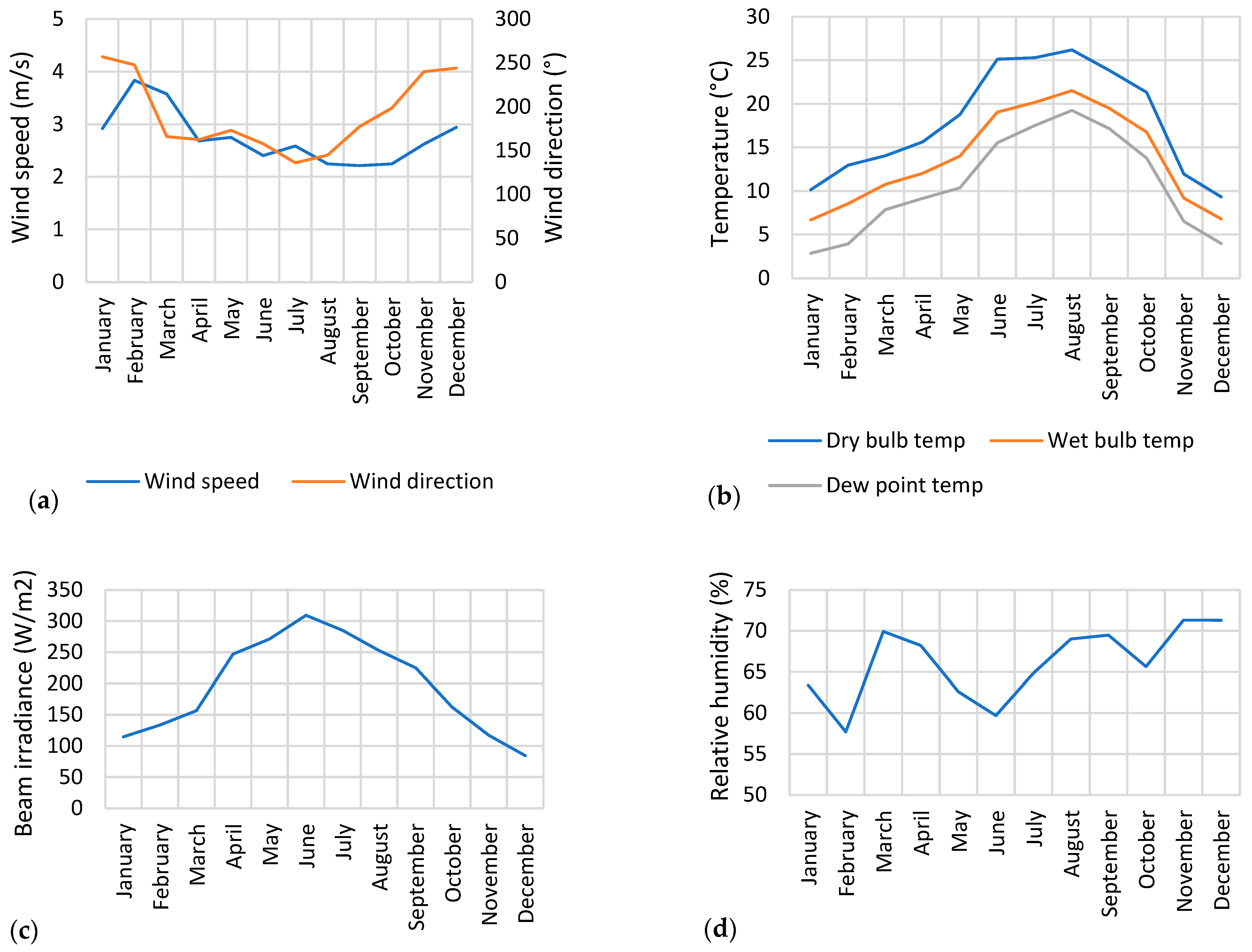
Weather information has been obtained from a weather station, specifically MISOL HP2550, which includes an anemometer installed on site. Regarding weather conditions, Figure 3a shows the wind speed at the site, over a year, with its speed being relatively constant. Figure 3b shows the annual dry bulb, wet bulb, and dew point temperature characteristics required by SAM, with the highest levels during summer months. Figure 3c shows the beam irradiance in W/m² at the site, with an annual beam irradiance of 2806 W/m², with June being the month with the highest beam irradiance (311 W/m²) and December the lowest beam irradiance (157 W/m²), and Figure 3d shows the relative humidity, which can be observed to be high throughout the year. This weather information has been implemented in SAM.

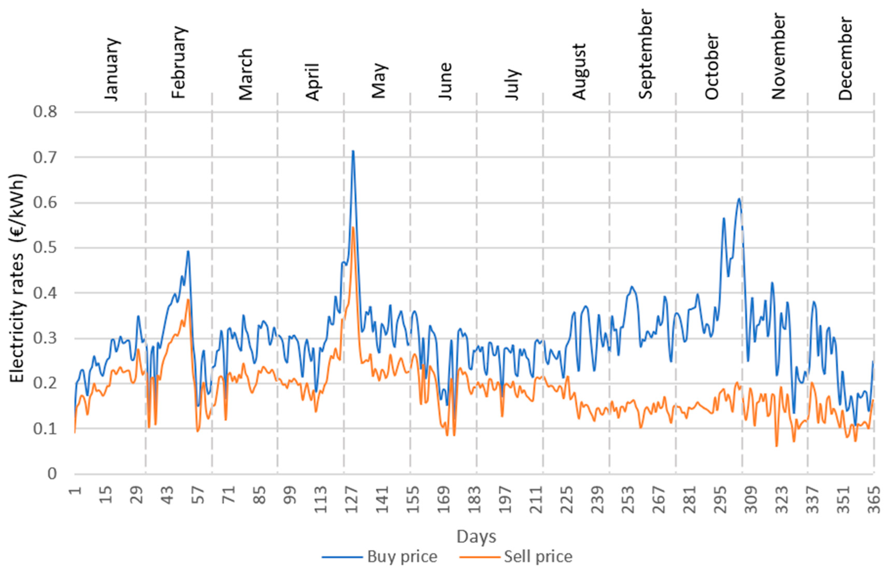
2.2.2. Electricity Rates

The electricity rates are required input in SAM to properly model the PV system. One-hour interval data of Spain’s daily electricity market rate have been downloaded from ESIOS (System Operator Information System, see Figure 4). The electricity billing has been configured in SAM as ‘Net billing’ because it is the one that most closely resembles the real installation.

2.2.3. Real PV System Data

The energy data of the PV system with a five-minute interval have been collected using the FusionSolar application, which monitors the installation. The energy that flows through the solar inverter, $E_{PV}$, the energy measured by the meter connected to the grid, $E_{grid}$ (which shows the electricity sent to the grid (positive) and received from the grid (negative)), and the load consumption, $E_{load}$, have been downloaded. The application reported some zero or error energy values. This is a common occurrence for measuring instruments that may go offline or malfunction from time to time. The dataset was screened for such values and set to the corresponding previous day values.

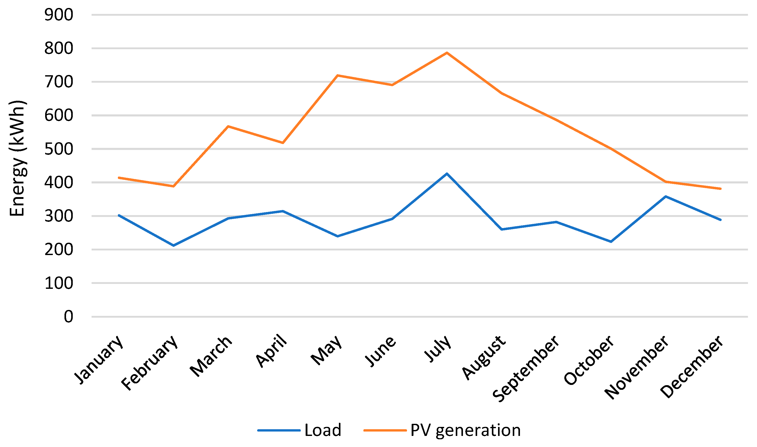
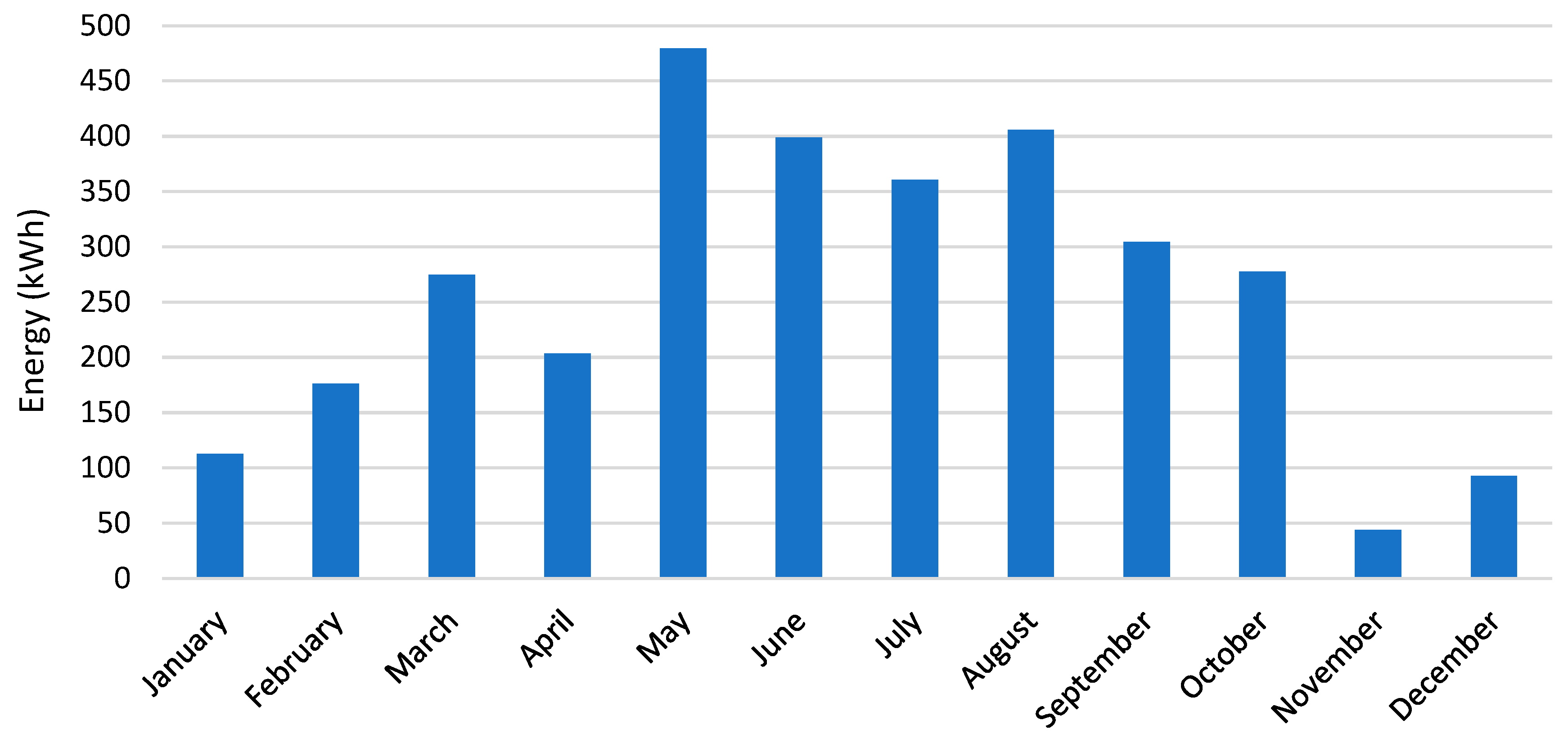
The load curve (see Figure 5) shows that the total annual consumption was 3491 kWh, with July being the month with the highest consumption, with 426 kWh, and February the month with the lowest consumption, with 212 kWh. The main consumers are air conditioning (30.4% with respect to the total), the electric water heater (20.0% with respect to the total), and the fridge (11.4% with respect to the total). The air conditioner is mainly used in winter and summer. The water heater consumes more energy in winter compared to summer (in January, it consumed 97.2 kWh, and in July, it consumed 42.10 kWh). The PV generation curve (see Figure 5) shows that the total annual energy generated was 6621 kWh, where July was the month with the highest value of 787 kWh and December was the month with the lowest generation of 381 kWh.

2.3. Data Filtering

The energy consumed by the load system, $E_{load}$, has been calculated through an energy balance according to Equation (1). E_grid is positive when energy is exported and negative when it is imported, and obviously the E_load is always positive when the PV is not producing energy and E_grid is negative when there is energy demand. The self-consumption energy, $E_{PV load}$, has been calculated employing Equation (2).

$$E_{load}=E_{PV}-E_{grid}$$

(1)

$$\left\{\begin{array}{cc}{E}_{PV load}=E_{PV}-E_{grid}\hfill & if E_{grid}>0\hfill \\ E_{PV load}=E_{PV}\hfill & if E_{grid}<;0\hfill \end{array}\right.$$

(2)

where $E_{PV}$ is the energy generated by the PV system, and $E_{grid}$ is the energy measured from/to the grid. In Equation (2), when there is surplus energy, the PV system is producing more energy than necessary to meet the demand, and thus the surplus is sent to the grid, $E_{grid}>0$. However, when the system has not been able to meet the demand, the grid must supply some energy, $E_{grid}<0$.

Then, all values obtained were transformed into one-hour intervals using Equation (3):

$$E_h={\displaystyle \sum }_{i=1}^n\frac{E_{h_i}}{60/5 }$$

(3)

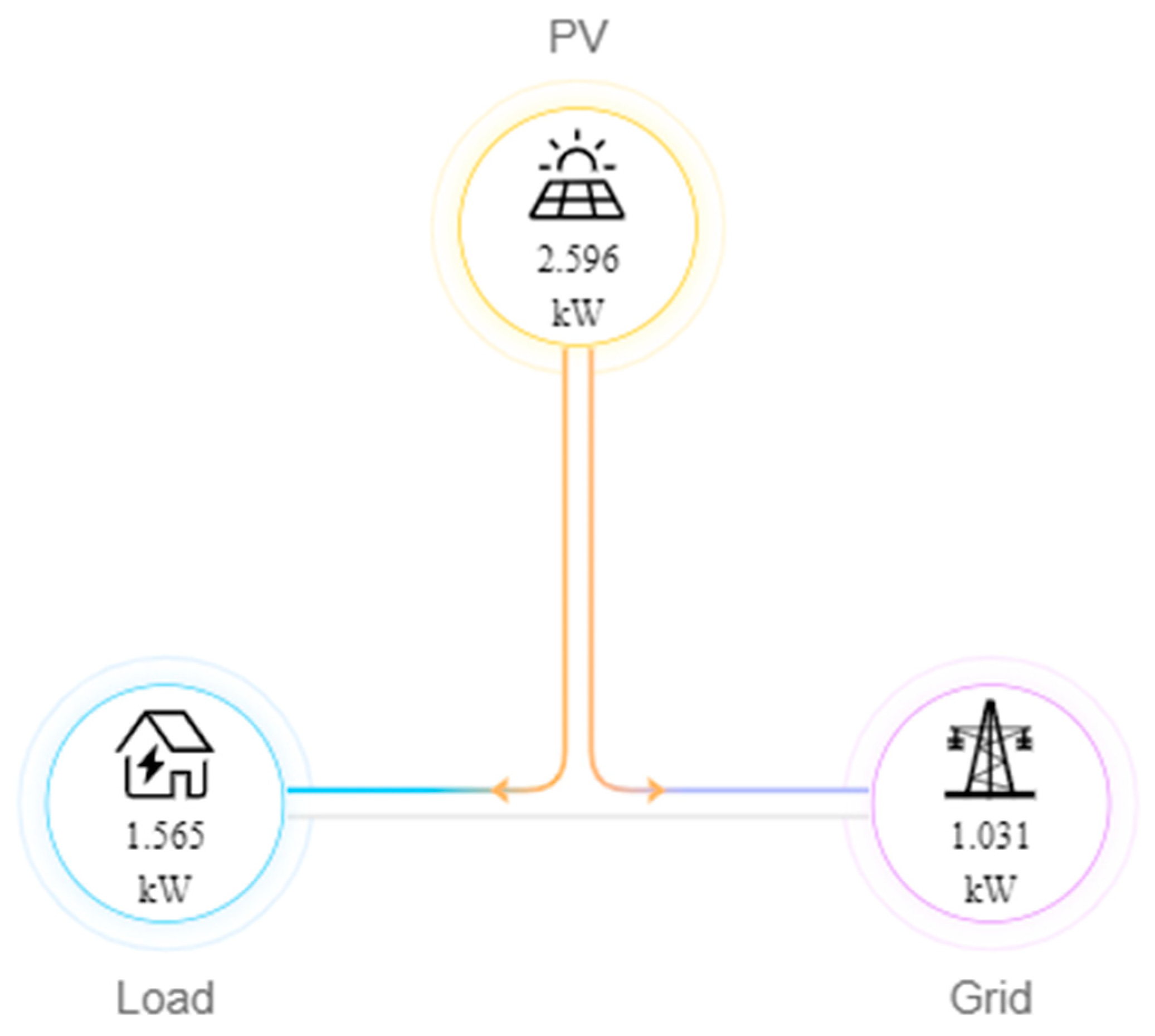
where $E_h$ is the hourly energy generated, and $i$ represents each 5 min time step. Figure 6 shows the components of the PV system analysed.

2.4. Scenario Development

To analyse the impact of higher DC to AC ratios, eleven DC to AC ratio scenario simulations for PV residential rooftop systems have been conducted (the current ratio of the PV system is 1.40, see

Table 3. DC to AC power ratios simulated. Rated P_AC is 3 kW.

PDC (kW)	${\mathit{r}}_{{\mathit{P}}_{\mathit{D}\mathit{C}-\mathit{A}\mathit{C}}}$
2.80	0.93
3.15	1.05
3.50	1.17
3.85	1.28
4.20	1.40
4.55	1.52
4.90	1.63
5.25	1.75
5.60	1.87
5.95	1.98
6.30	2.10

). To increase the DC to AC ratio, the AC output inverter rating has been held constant while the rated DC capacity of the solar array has been increased. It can be observed that DC to AC ratios do not increase progressively since the increase in the DC array must be consistent with the power characteristics of the PV panels used in the current installation. In this study, the inverter DC to AC power ratio ($r_{P_{DC-AC}})$ is defined as Equation (4):

$$r_{P_{DC-AC}}=\frac{P_{DC capacity}}{P_{AC capacity}}$$

(4)

where $P_{DC capacity}$ is the input power of the solar inverter from the PV field, and $P_{AC capacity}$ is the output power of the solar inverter, that is the energy from the whole PV system.

Values above 4500 W (maximum recommended capacity of the inverter manufacturer) were used to observe the influence of higher DC to AC ratios, since when the inverter receives higher powers from the photovoltaic field, it modifies the MPP, limiting the input power to 4500. With a higher installed DC power, it can be observed that the inverter is able to capture more energy during more hours throughout the day.

Where $P_{DC capacity}$ is the maximum rated capacity power output of the PV system and $P_{AC capacity}$ is the inverter’s maximum AC power output.

In addition, different scenarios were considered by varying the DC to AC ratio, a 30° step-azimuth (see

Table 4. 30° step-azimuth variation.

Azimuth Variation
0°
30°
60°
90°
120°
150°
180°
202°
210°
240°
270°
300°
330°

), and a 10° step-slope variation (see

Table 5. 10° step-slope variation.

Slope Variation
0°
10°
20°
30°
40°
50°
60°
70°
80°
90°

), resulting in the simulation of over 1000 scenarios. Therefore, the sensitivity of the results due to slope, azimuth, and DC to AC ratio variation was tested. Lower slopes represent a project that seeks to maximize summer generation, while higher slope angles are more suitable for increased winter generation.

Several assumptions have been made to best isolate the impacts of inverter clipping. The system was arranged in a double subarray with no self-shading and no external shading. Soiling losses of 5% equally applied to each month have been assumed. DC losses totalled 4.4% and consisted mainly of module mismatch losses (2%) and DC wiring losses (2%). AC losses of 1% attributable to wiring have been considered.

2.5. System Performance

Simulation results were obtained annually, monthly, and daily to provide a complete picture of how the increase in the DC to AC ratio affects the system operation. Two optimisation criteria have been studied: maximising the performance ratio as an energetic criterion and minimising the discounted payback period as an economic criterion. The total system generation is the sum of inverter AC output throughout a year, taking into account AC losses.

To evaluate the results, different energy concepts were used. The capacity factor (CF (%)) is the ratio of the system’s predicted electrical output in the first year of operation to the nameplate output, which is equivalent to the quantity of energy the system would generate if it operated at its nameplate capacity for every hour of the year. Therefore, for PV systems, the capacity factor is an AC to DC value, as shown in Equation (5):

$$CF=\frac{E_{AC total}}{P_{DC capacity}·8760}$$

(5)

where $E_{AC total}$ is the net annual energy in kWh/year in AC, $P_{DC capacity}$ is the system capacity in kW (that is, the system’s DC nameplate capacity), and 8760 is represented in h/year.

Power lost due to clipping, $P_{clip}$ (kW), is a power limit loss that occurs in time steps when the inverter’s AC power output exceeds the total inverter nameplate AC capacity. During these time steps, SAM adjusts the inverter output to the inverter-rated capacity (it does not adjust the inverter’s input voltage). Then, the generation lost due to clipping is the sum of $P_{clip}$ over time, as Equation (6) explains:

$$\left\{\begin{array}{cc}Pclip=P_{AC}-P_{AC capacity},\hfill & if P_{AC}>P_{AC capacity} \hfill \\ Pclip=0,\hfill & if P_{AC}\le P_{AC capacity}\hfill \end{array}\right.$$

(6)

where $P_{AC}$ is the AC power generation, and $P_{AC capacity}$ is the AC capacity.

The inverter model equation used by SAM to calculate the $P_{AC}$ power [18] is represented by Equation (7). Moreover, SAM considers that the inverter is operating in night mode when the DC input power is less than the operating power losses ($P_{DC}<P_{SO}$); thus, Equation (8) is applied at night.

$$P_{AC}=\frac{P_{AC capacity}}{P_{DC capacity}-P_{S,0}}\ast {\left(P_{DC}-P_{SO,0}\right)}^2$$

(7)

where, $P_{AC capacity}$ is the maximum AC power, $P_{DC capacity}$ is the maximum DC power, $P_{S,0}$ is the power consumption during operation, and $P_{SO,0}$ is the inverter power consumption loss.

$$P_{AC}=-P_{nt,0}$$

(8)

where $P_{nt,0}$ is the power consumption at night.

Additionally, the system performance has been evaluated using the so-called effective energy. It represents the energy values from the difference of the overproduction of energy with respect to the base case minus the clipping losses ($E_{clip}$), see Equation (9):

$$E_{effective}=\left(E_{PV}-E_{PV base case}\right)-E_{clip}$$

(9)

where $E_{PV base case}$ is the energy generated and supplied by the PV system in the base case, which is the current installation case (azimuth of 202°, slope of 20.5°, and DC to AC ratio of 1.4).

Finally, the discounted payback period is used as an economic criterion. The discounted payback period (DPB) is used to determine the number of years (n) it takes to reach the break-even point from the initial expenditure, discounting future cash flows and considering the time value of money, according to Equation (10) [19]:

$${{\displaystyle \sum }}_n\frac{\Delta I_n}{{\left(1+d\right)}^n}\le {{\displaystyle \sum }}_n\frac{\Delta S_n}{{\left(1+d\right)}^n}$$

(10)

where $n$ represents the number of years, DPB is the minimum number of years required for the discounted sum of annual net savings to equal the discounted incremental investment costs, $\Delta I$ are the incremental investment costs, $\Delta S$ are the annual savings net of future annual costs (for instance, $\Delta S$ equals the incremental energy costs, incremental nonfuel operation, maintenance, and repair costs, incremental repair and replacement costs, minus the incremental salvage costs), and $d$ is the annual nominal discount rate. The annual discount rate considered was 8.35%.

3. Results

This section explains the results obtained from data validation, which ended up being successful. Additionally, energy production, clipping losses, and system sensitivity to slope and azimuth variation are shown in detail.

3.1. Data Validation

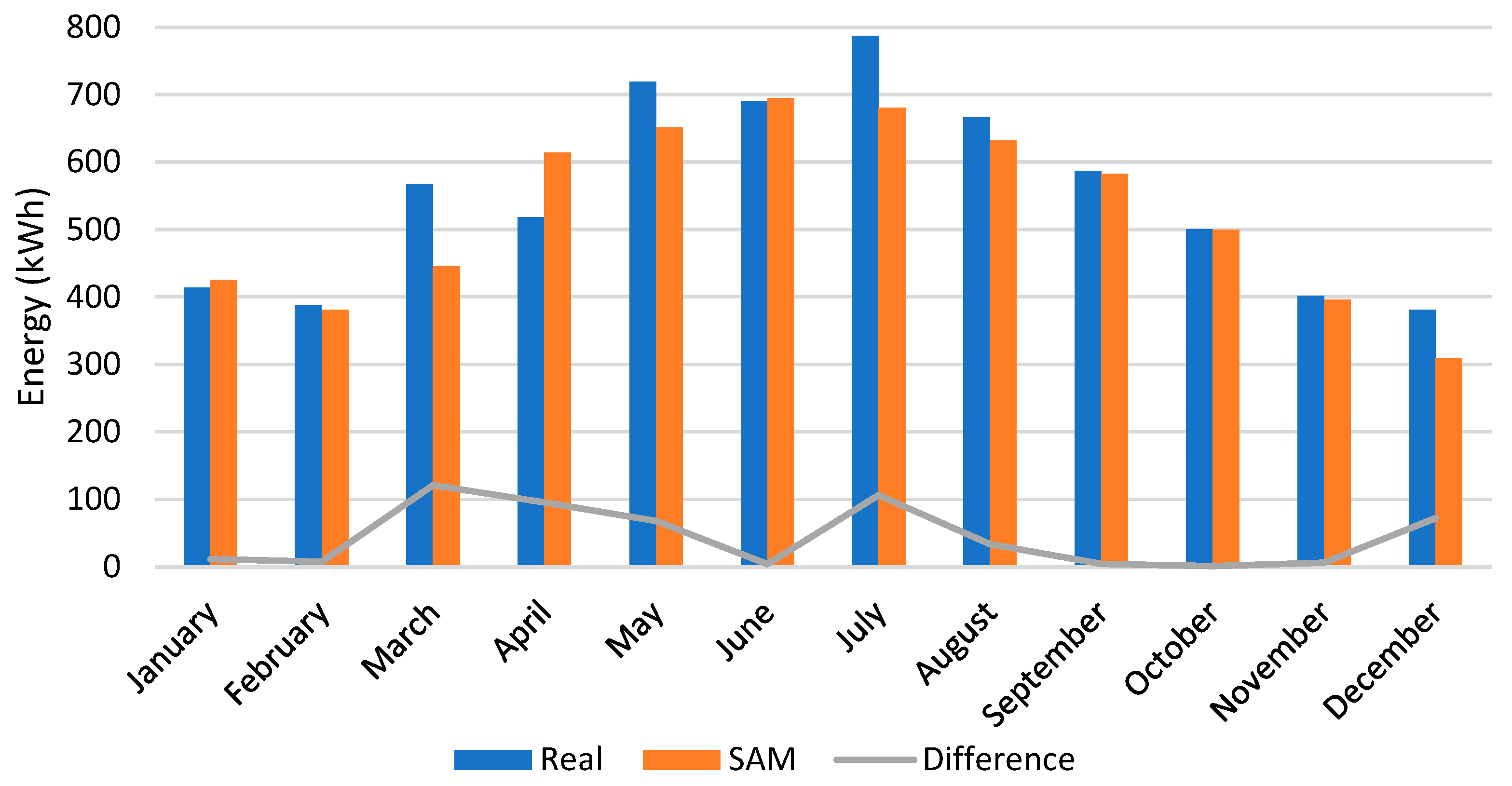
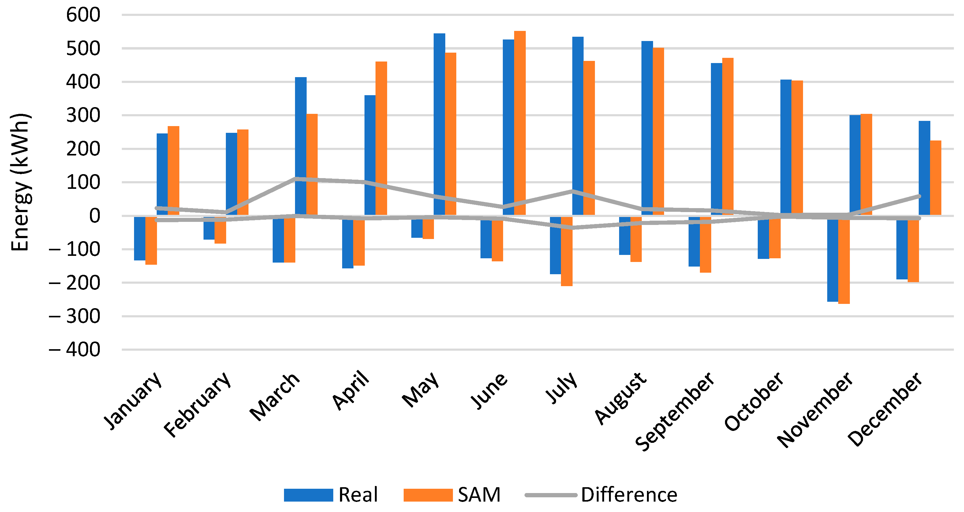
SAM result data files were reviewed for completeness and additionally validated. Results were compared with the data previously obtained from the FusionSolar application, based on the calculations performed on these data, and finally filtered. Figure 7 compares the filtered and modelled data regarding the PV system AC energy generation. The biggest difference between the real generated energy (567 kWh) and the energy of the SAM simulated model (460 kWh) occurred in March, with an error of 18.8%. The system has been considered valid since the average monthly error was 7.7%, and the error corresponding to the annual energy produced was 4.7%.

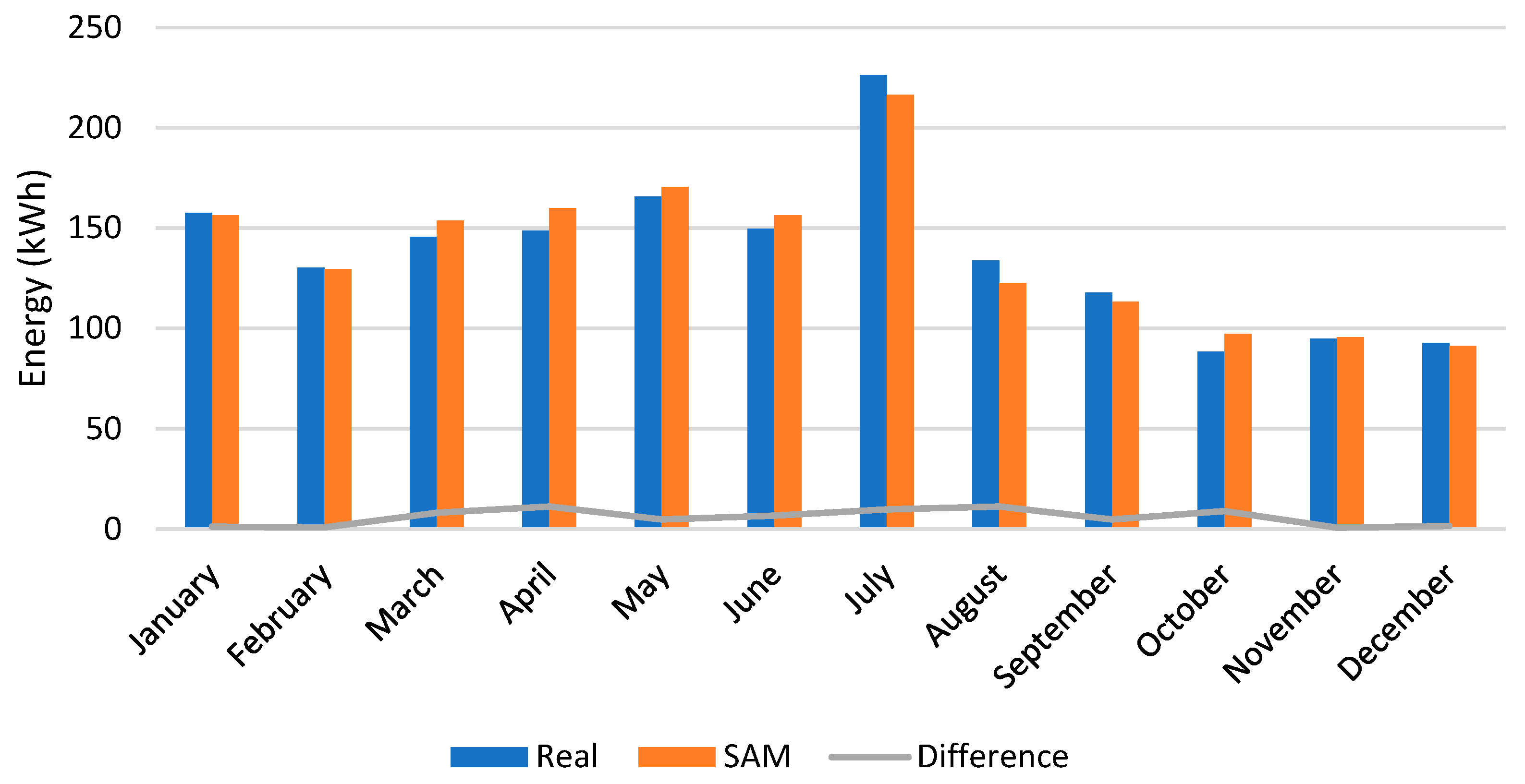
The electricity that flows directly from the PV system to the load was also compared, obtaining values quite similar, with differences of less than 10%, as shown in Figure 8, which corresponds to 9 kWh.

Moreover, Figure 9 shows the differences between the real energy sent to/received from the grid. When the PV system cannot meet the demand, the necessary energy is taken from the grid (negative values in Figure 9). Conversely, when the PV system has a surplus after having covered the demand, the surplus energy is sent to the grid (positive values in Figure 9).

The energy supplied from the grid shown in Figure 9 had a maximum difference in July of 21%, and the energy delivered to the grid in Figure 9 had a maximum difference in March of 29%. These values may be slightly higher than the previous ones but have still been considered acceptable.

Considering the results obtained from the simulation, they have been considered acceptable, and the modelled system has been validated.

From the results in Figure 9, the net balance can be obtained. As positive values are reported, it can be concluded that the current PV installation is self-sustainable, see Figure 10.

3.2. System Output and Clipping

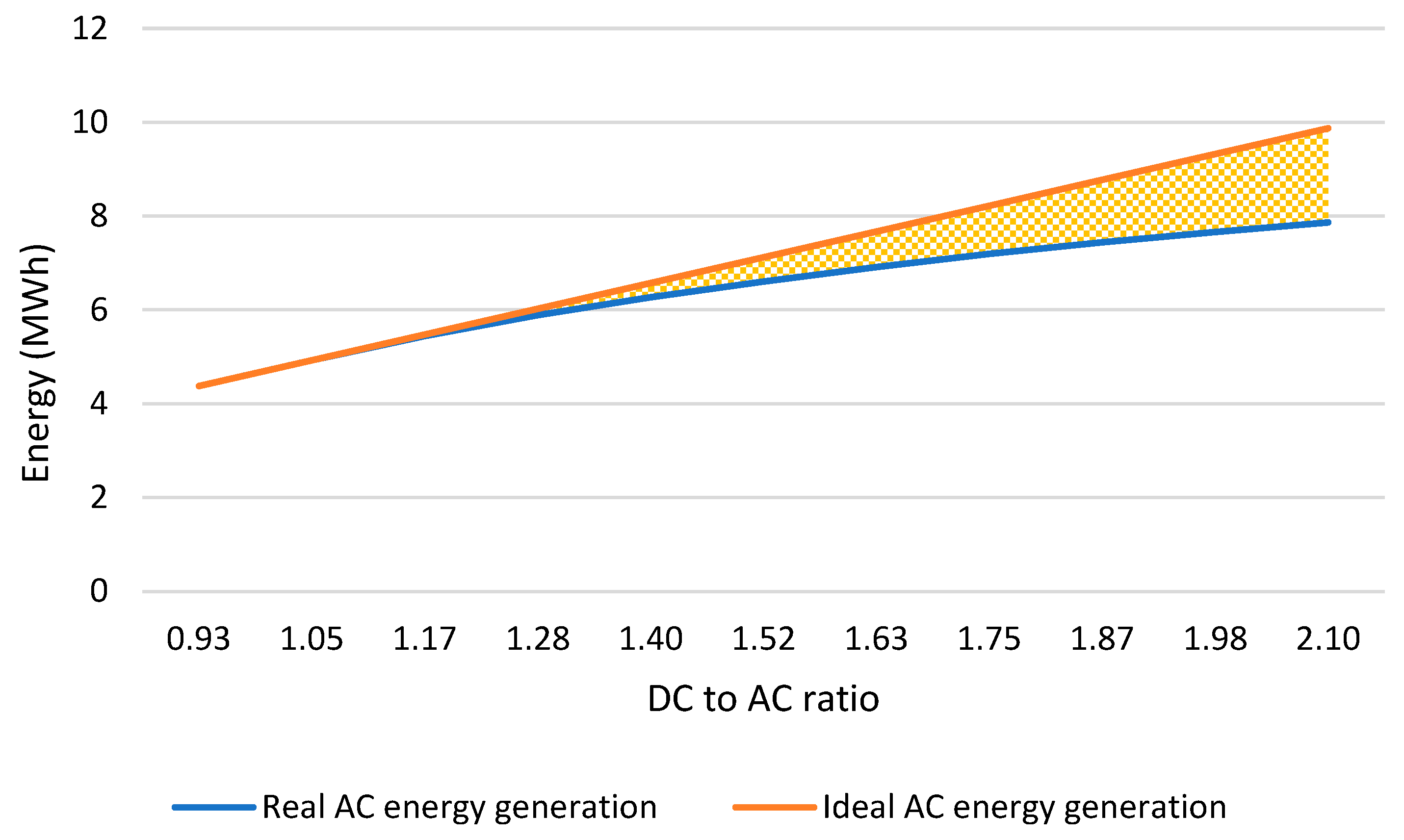
The impact of clipping as a function of the DC to AC ratio is shown in Figure 11 via Table 3 simulations. Figure 11 graphs the real AC energy generation against the ideal AC energy generation as if there were no clipping loss effects at the inverter. The shaded area represents the clipping produced by the inverter power limit. It can be observed that the greater the DC to AC ratio, the more significant the clipping losses. The point at which losses started to occur was for a DC to AC ratio of 1.17. 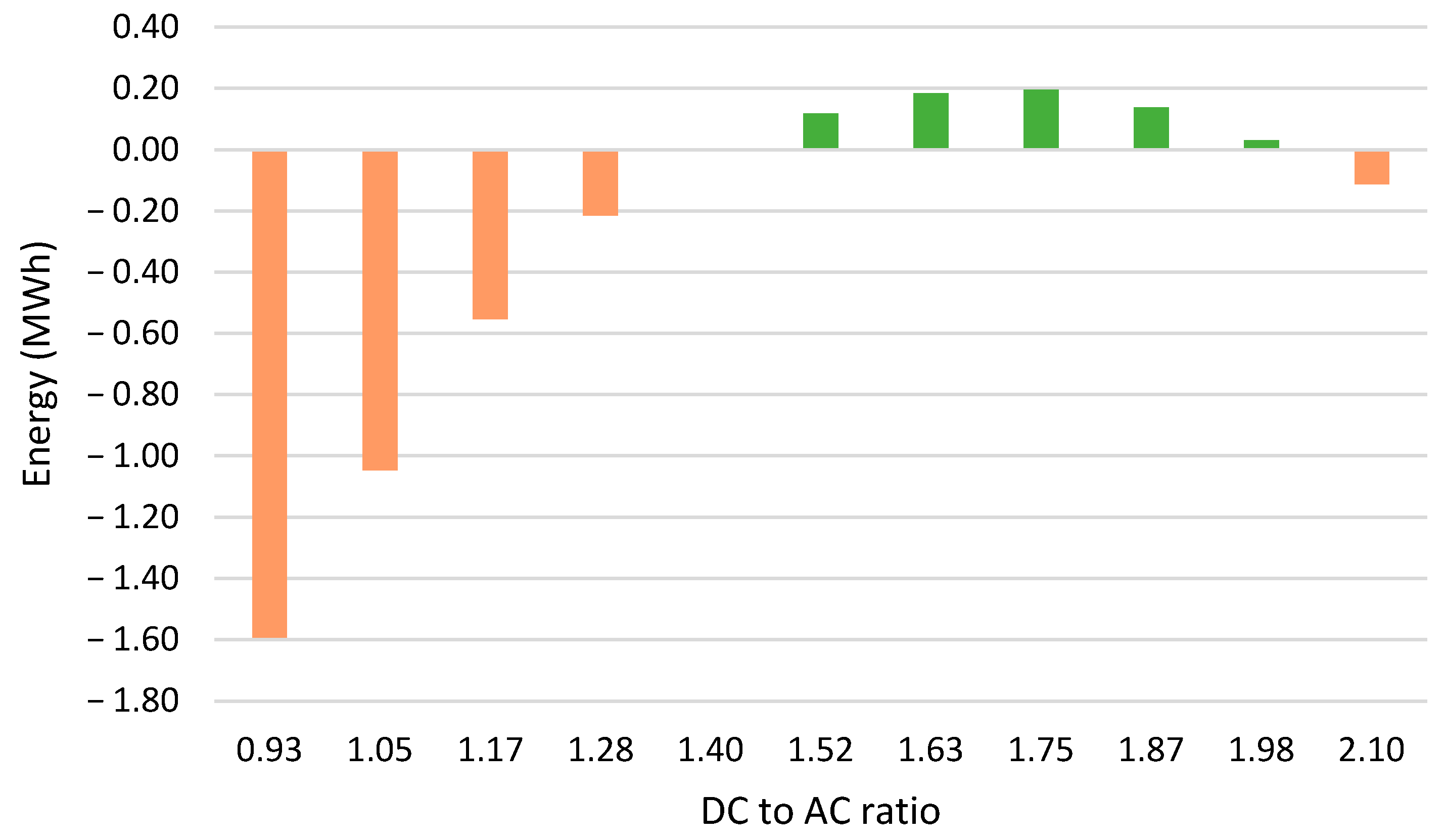Similarly, Figure 12 shows whether the variation of the DC to AC ratio was an effective solution concerning the base case, representing the energy values from the difference of the overproduction of energy concerning the base case minus the clipping losses ($E_{clip}$), as shown in Equation (9). The positive values in the figure mean that the energy that has been generated in excess (in the case under study) with respect to the base case was greater than the clipping losses that may be present; in short, more energy was obtained with solutions with positive values. Green columns show the best DC to AC ratios, between 1.52 and 1.98, whereas red columns show the worst DC to AC ratios, between 0.93, 1.28, and 2.10. Concerning the base case, 1.40 was equal to zero as it represents the base case.

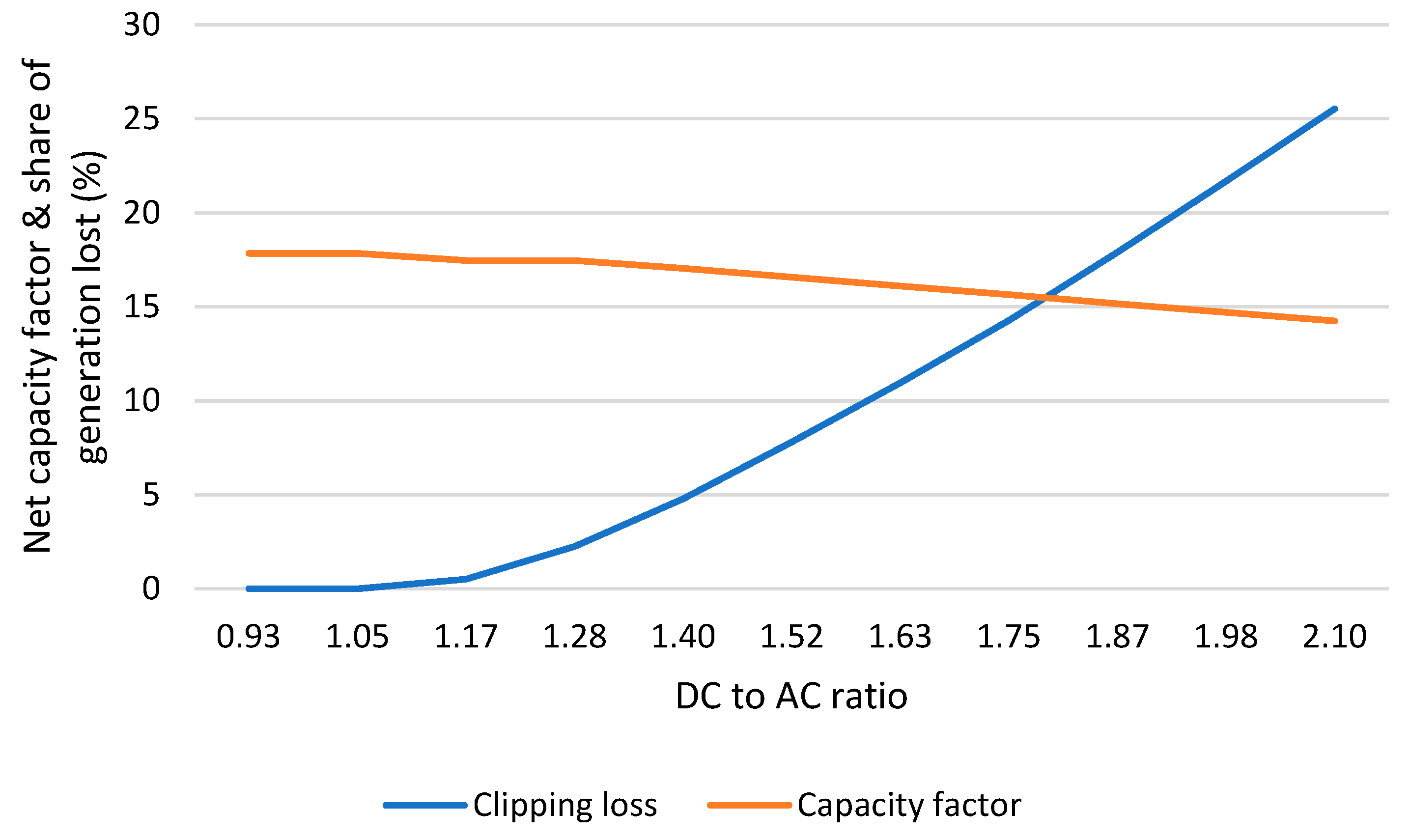
On the other hand, Figure 13 shows that the capacity factor decreased linearly as the DC to AC ratio increased against a quasi-exponential increase in clipping losses. Clipping losses increased from 0.51% to 25.53%. These clipping losses reduced the annual net capacity factor, calculated in terms of DC-rated capacity, from 17.46% to 14.25%.

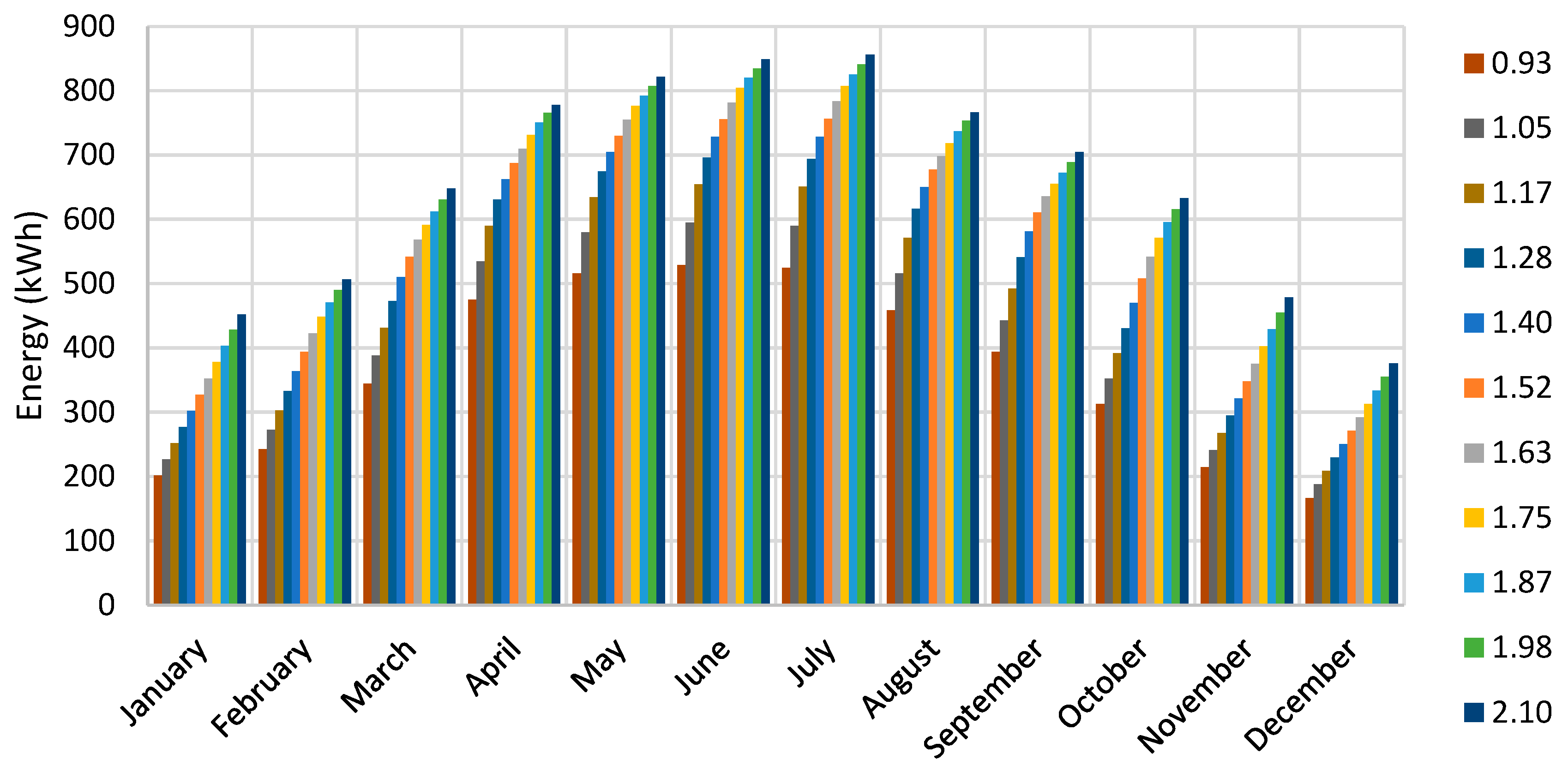
3.3. Monthly Variation in Energy Generation and Clipping Losses

Figure 14 shows the monthly energy generation trend throughout the year for each DC to AC ratio. It can be seen that winter months had the lowest energy generation, particularly in December, with values ranging from 167 kWh to 376 kWh for each DC to AC ratio in incremental order. The summer months, conversely, were notable for their high energy generation values, especially June with values ranging from 529 kWh to 849 kWh for each DC to AC ratio in incremental order.

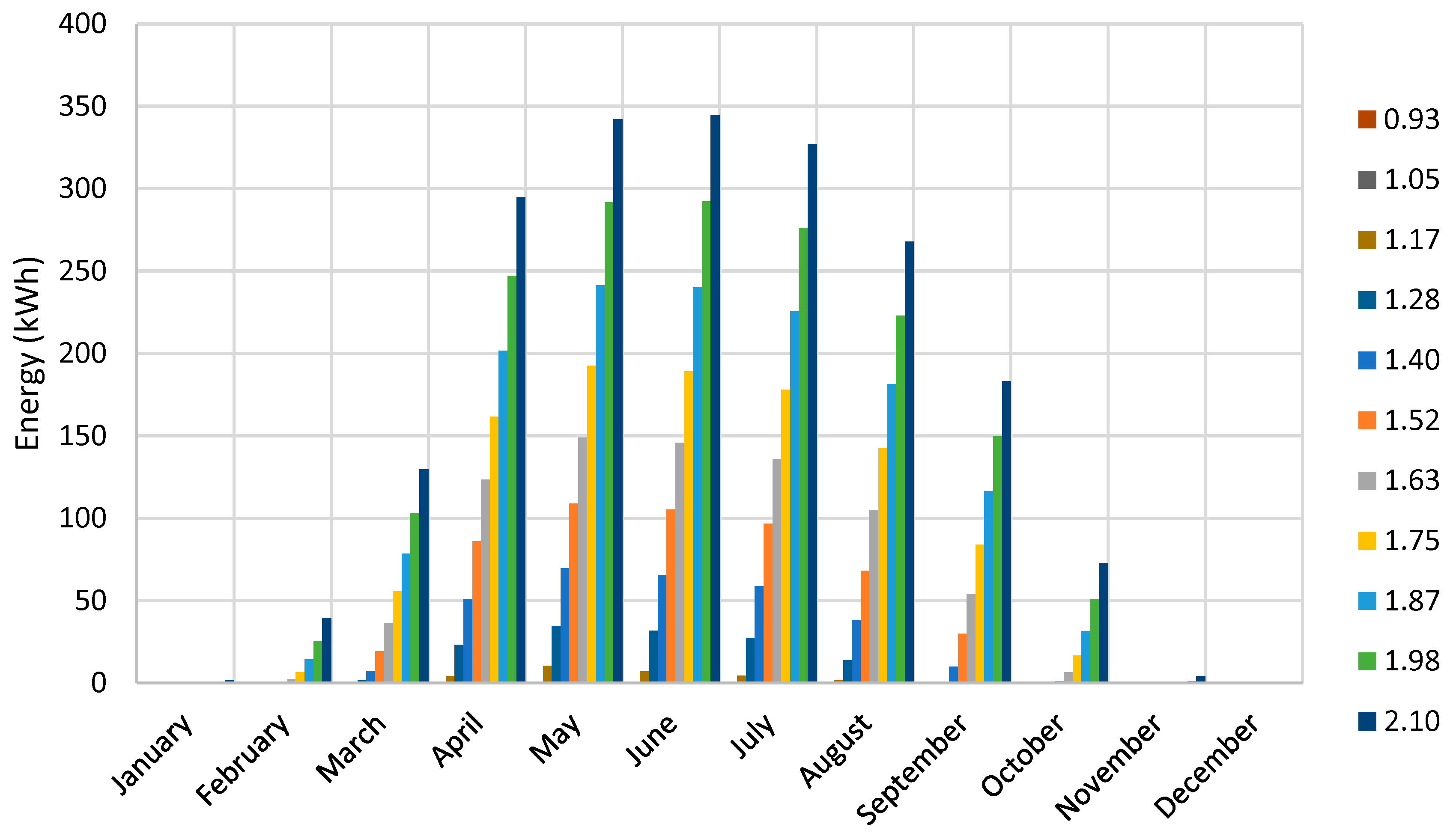
Concerning the inverter clipping losses associated with energy generation, a similar trend can be observed in Figure 15 as in Figure 14, where the lowest values were found in winter, particularly in December, with no clipping losses for any DC to AC ratio, whereas the highest values were found in summer, especially in May, with 10.31 kWh, 34.66 kWh, 69.59 kWh and 108.95 kWh, 148.89 kWh, 192.54 kWh, and 241.37 kWh for DC to AC ratios of 1.17, 1.28, 1.40, 1.52, 1.63, 1.75, and 1.87, respectively, and in June for higher ratios with 292.35 kWh and 344.84 kWh for DC to AC ratios of 1.98 and 2.10, respectively.

In addition, it can also be noticed that as the DC to AC ratio increased in the PV system, the difference concerning the previous DC to AC ratio clipping losses increased as well.

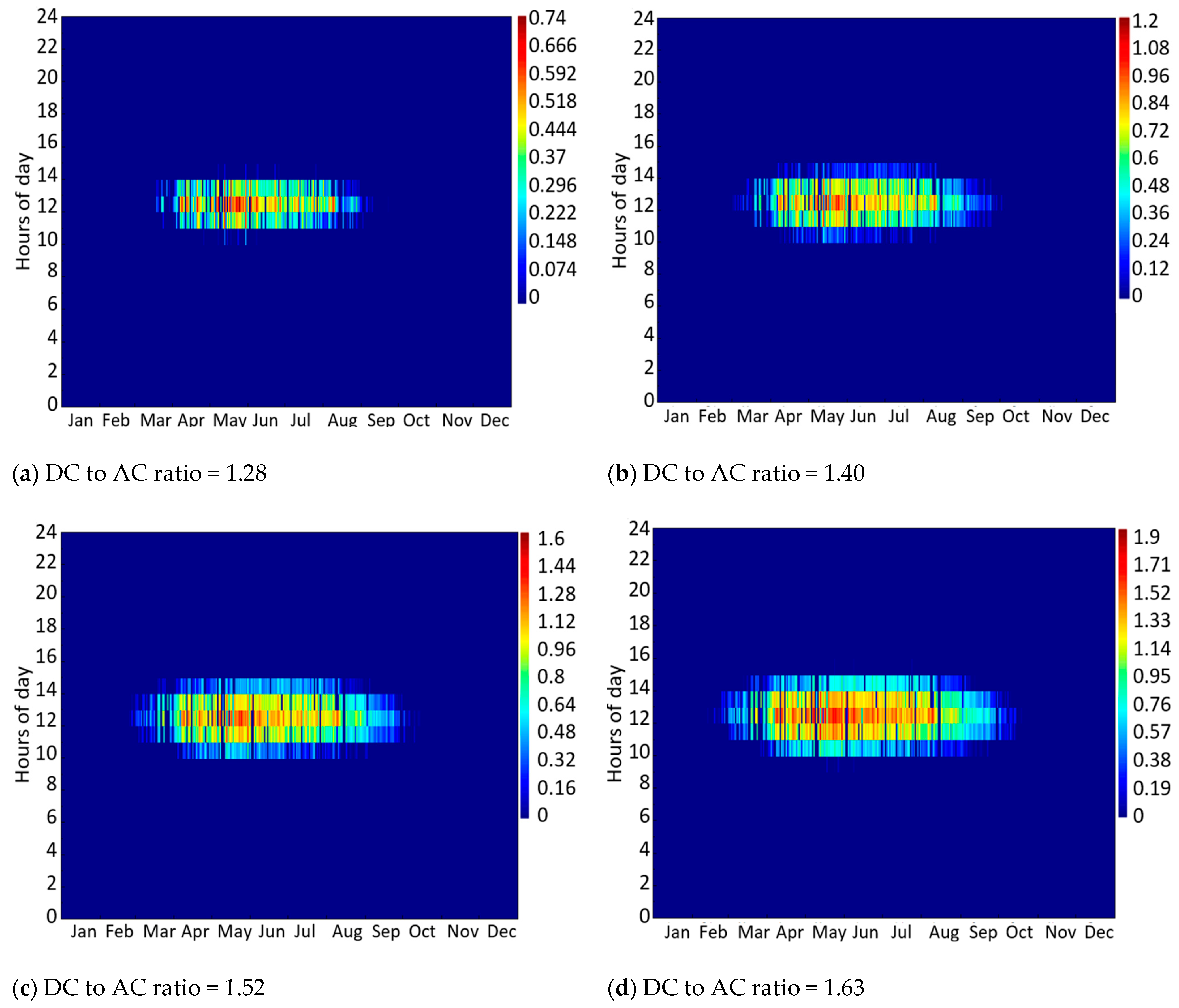
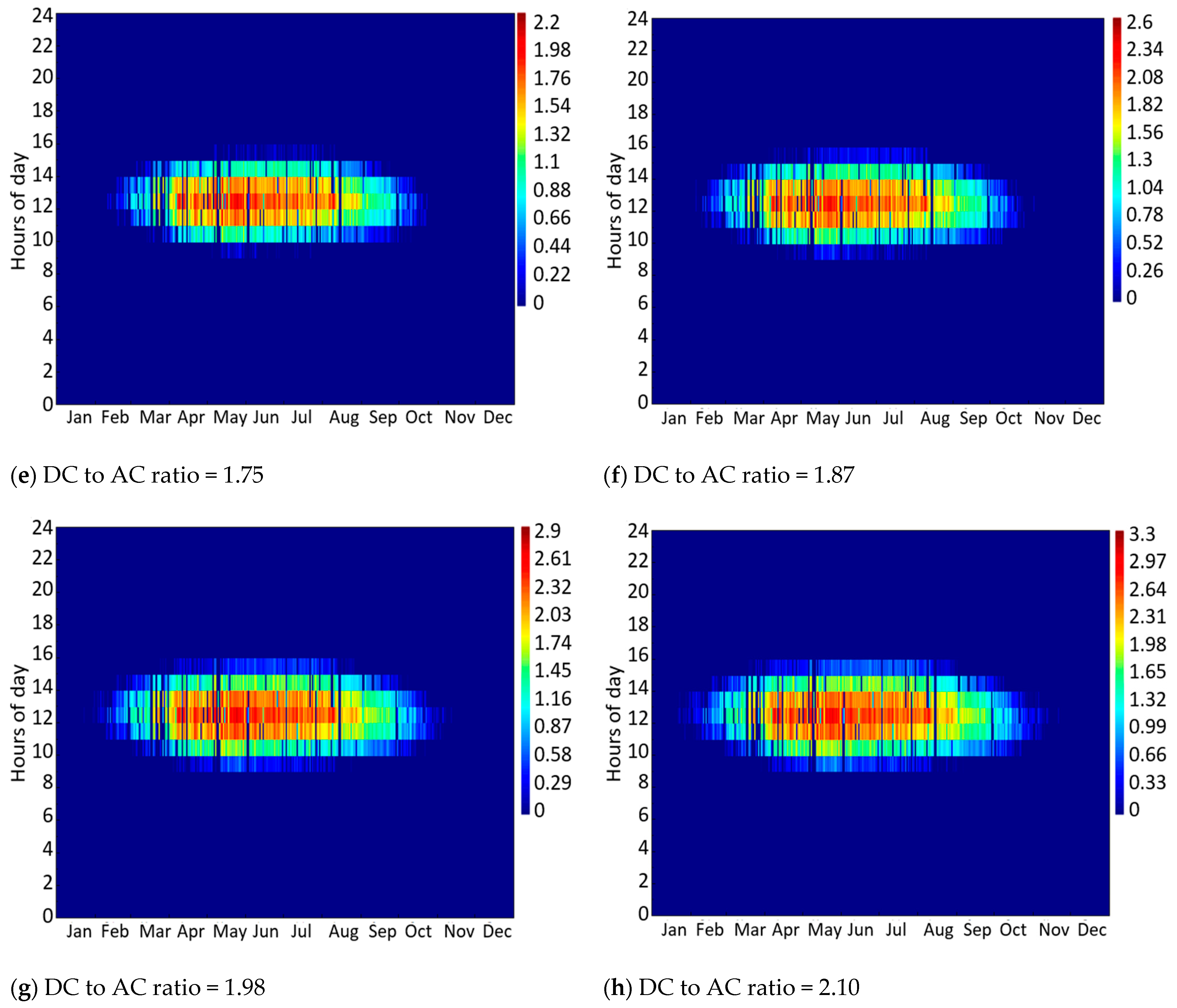
3.4. Daily and Seasonal Clipping Losses

While Figure 15 provides important details on seasonal trends, it does not illustrate the inter-day variations in clipping losses. Figure 16 heat maps show the distribution of clipping losses each hour for each month. As expected for all months, the highest clipping losses occurred at mid-day hours since radiation values are the highest at those hours. Regarding seasonal evolution, the highest shares occurred in spring, between March, April, and June, and the lowest shares occurred in winter, between November, December, and January, resulting consistent with the assumption for this system, which has been a fixed slope angle similar to the site’s latitude. Moreover, it can be observed that the higher the DC to AC ratio, the greater the hourly clipping losses.

For a more in-depth study of clipping losses, the day with the highest losses for each DC to AC ratio has also been analysed, 2 May, comparing a real energy production day and an ideal energy production day with no inverter AC power limit.

Table 6. Examples of inverter clipping on 2 May for different inverter DC to AC ratios.

DC to AC Ratio	Maximum Power (kW)		Maximum Energy (kWh)		Energy Losses (%)
	Real Case	Ideal Case	Real Case	Ideal Case
0.93	2.56	2.56	17.56	17.56	0.0%
1.05	2.88	2.88	19.76	19.76	0.0%
1.17	2.97	3.20	21.64	21.96	1.5%
1.28	2.97	3.53	22.93	24.16	5.1%
1.40	2.97	3.85	23.94	26.37	9.2%
1.52	2.97	4.17	24.69	28.58	13.6%
1.63	2.97	4.50	25.45	30.79	17.3%
1.75	2.97	4.82	26.21	33.01	20.6%
1.87	2.97	5.14	26.77	35.22	24.0%
1.98	2.97	5.47	27.14	37.43	27.5%
2.10	2.97	5.79	27.52	39.65	30.6%

shows the variation of the maximum power in kW, maximum energy in kWh, and energy losses in percentage for each DC to AC ratio simulated (from 0.93 to 2.10), at a real case (with inverter clipping losses) and at an ideal case (without inverter clipping losses). Thus, by comparing the real vs. the ideal cases, the magnitude of the energy lost due to clipping can be deduced, and the higher the DC to AC ratio, the maximum power saturates according to the solar inverter characteristics, and more energy is produced, but more energy is also lost. This demonstrates, as in Figure 12, that sometimes the increase of the DC to AC ratio is not an effective solution when more energy generation is sought.

3.5. Sensitivity to Azimuth

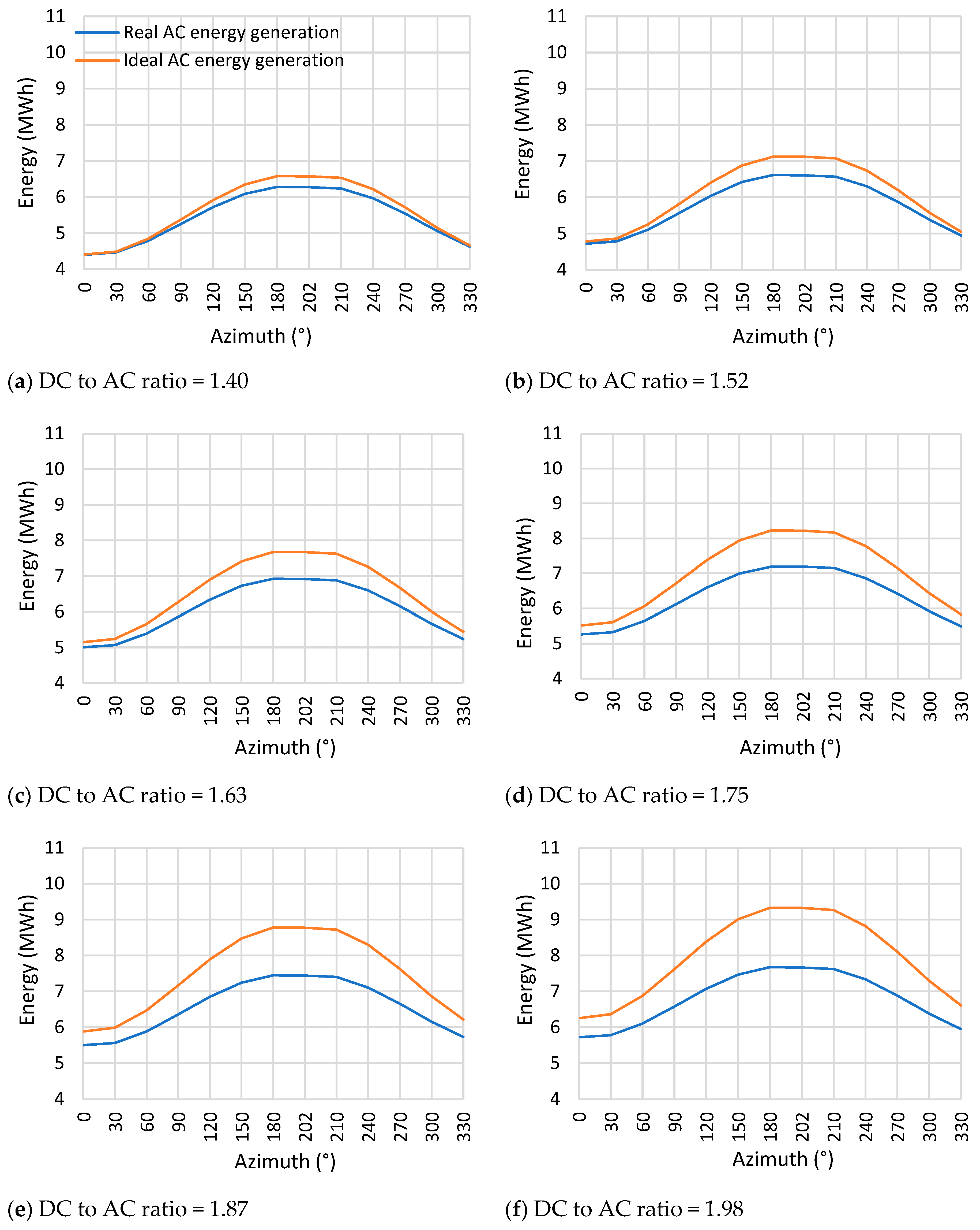
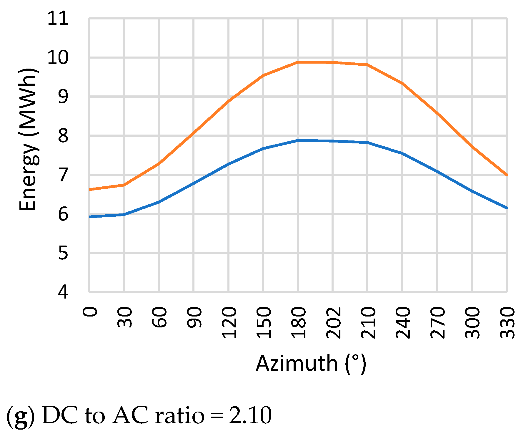
Simulations corresponding to Table 4 scenarios with a 30° step-azimuth variation from 0° to 330° for each DC to AC ratio, a fixed slope of 20.5°, and a constant DC to AC ratio of 1.40 were evaluated to analyse the PV system’s sensitivity against azimuth changes and to monitor how clipping losses are modified.

3.5.1. Energy Generation

Figure 17 only shows the graphs from the DC to AC ratio of 1.40 onwards, since this is when clipping losses first became significant. As expected, it shows that as the DC to AC ratio increased, the energy production increased, contributing negatively to an increase in the inverter clipping losses. The highest clipping losses were found in the central azimuths of the graphs, those corresponding to a southern layout due to the location of the PV system, which favours a greater capture of solar radiation for azimuths close to 180°, while at opposite angles, such as 0°, the capture was much lower, and hence the generation of energy and its corresponding losses were lower as well.

However, as already obtained, the increase in energy generation (overproduction in comparison to the base case) may not only mean an effective solution and the magnitude of the values must also be taken into account. In order to determine whether it is worth increasing the DC to AC ratio and modifying the azimuth, the new energy values must be compared regarding the energy overproduction and the magnitude of the effective energy from Equation (8). Green cells in

Table 7. Effectiveness of the DC to AC ratio regarding energy generation with a variable azimuth and a fixed slope of 20.5°, in kWh.

Azimuth	DC to AC Ratio *
	0.93	1.05	1.17	1.28	1.40	1.52	1.63	1.75	1.87	1.98	2.10
0°	−3031	−2663	−2295	−1928	−1581	−1312	−1106	−957	−849	−780	−742
30°	−2981	−2607	−2233	−1860	−1521	−1263	−1073	−934	−835	−773	−745
60°	−2741	−2337	−1932	−1542	−1237	−1009	−854	−743	−670	−640	−648
90°	−2393	−1946	−1500	−1117	−845	−654	−530	−453	−425	−434	−480
120°	−2033	−1541	−1063	−705	−447	−296	−203	−153	−157	−216	−306
150°	−1742	−1213	−721	−373	−145	−1	70	77	37	−42	−161
180°	−1590	−1042	−547	−209	13	141	196	191	147	54	−88
202°	−1594	−1046	−554	−215	−	118	184	197	138	31	−113
210°	−1621	−1077	−586	−246	−31	90	159	165	113	10	−128
240°	−1830	−1312	−830	−485	−259	−104	−42	−32	−59	−118	−211
270°	−2166	−1689	−1222	−856	−605	−430	−329	−283	−280	−309	−374
300°	−2545	−2116	−1688	−1294	−1005	−793	−648	−565	−522	−507	−525
330°	−2867	−2478	−2090	−1703	−1371	−1125	−938	−806	−727	−680	−659

* Green cells represent effective solutions, while red cells are not as effective.

represent effective solutions, while red cells are not as effective. It was deduced that the best solutions require an azimuth of 180°, and a DC to AC ratio between 1.63 and 1.75.

If one had only examined the real AC energy generation graphs from Figure 17, one would have believed that the best solution is to have a ratio of 2.10 with an azimuth of 180° as it is the solution that generated the most energy. However, it is not the most effective scenario compared to the base case due to the high losses it entails, energetically speaking.

In addition, it must be noted that the results show that the azimuth value greatly affected power generation, as can be evidenced by the significant values shown in the graphs and tables within this section.

3.5.2. Discounted Payback Period

The economic point of view has also been considered. Thus, the discounted payback period has been examined as the reference economic parameter (see

Table 8. Discounted payback period (years) of the DC to AC ratio regarding energy generation with a variable azimuth and a fixed slope of 20.5°.

Azimuth	DC to AC Ratio *
	0.93	1.05	1.17	1.28	1.40	1.52	1.63	1.75	1.87	1.98	2.10
0°	11.7	11.9	12.1	12.2	12.4	12.7	13.1	13.6	14.2	14.8	15.5
30°	11.3	11.5	11.6	11.8	12.0	12.3	12.8	13.3	13.8	14.5	15.2
60°	10.1	10.2	10.4	10.5	10.8	11.2	11.6	12.1	12.7	13.3	13.9
90°	8.8	9.0	9.1	9.3	9.6	10.0	10.4	10.9	11.4	11.9	12.5
120°	7.9	8.0	8.1	8.3	8.6	9.0	9.4	9.9	10.3	10.9	11.4
150°	7.3	7.4	7.5	7.7	8.0	8.4	8.8	9.2	9.7	10.2	10.7
180°	7.0	7.1	7.3	7.5	7.8	8.2	8.6	9.0	9.4	9.9	10.4
202°	7.0	7.2	7.3	7.5	7.9	8.2	8.6	9.0	9.5	9.9	10.5
210°	7.1	7.2	7.4	7.6	7.9	8.3	8.7	9.1	9.5	10.0	10.5
240°	7.6	7.7	7.8	8.1	8.4	8.8	9.2	9.6	10.1	10.6	11.1
270°	8.4	8.6	8.7	8.9	9.2	9.6	10.0	10.5	11.0	11.6	12.1
300°	9.7	9.8	9.9	10.1	10.4	10.8	11.2	11.7	12.3	12.8	13.5
330°	11.0	11.1	11.3	11.4	11.6	12.0	12.4	12.9	13.5	14.1	14.8

* Green cells represent effective solutions, while red cells are not as effective.

). As expected, the lower the DC to AC ratio, the lower the discounted payback period since fewer PV panels are required. In terms of azimuth variation, lower discounted payback periods were seen at 180°, as more energy was generated due to favourable angles.

3.6. Sensitivity to Slope

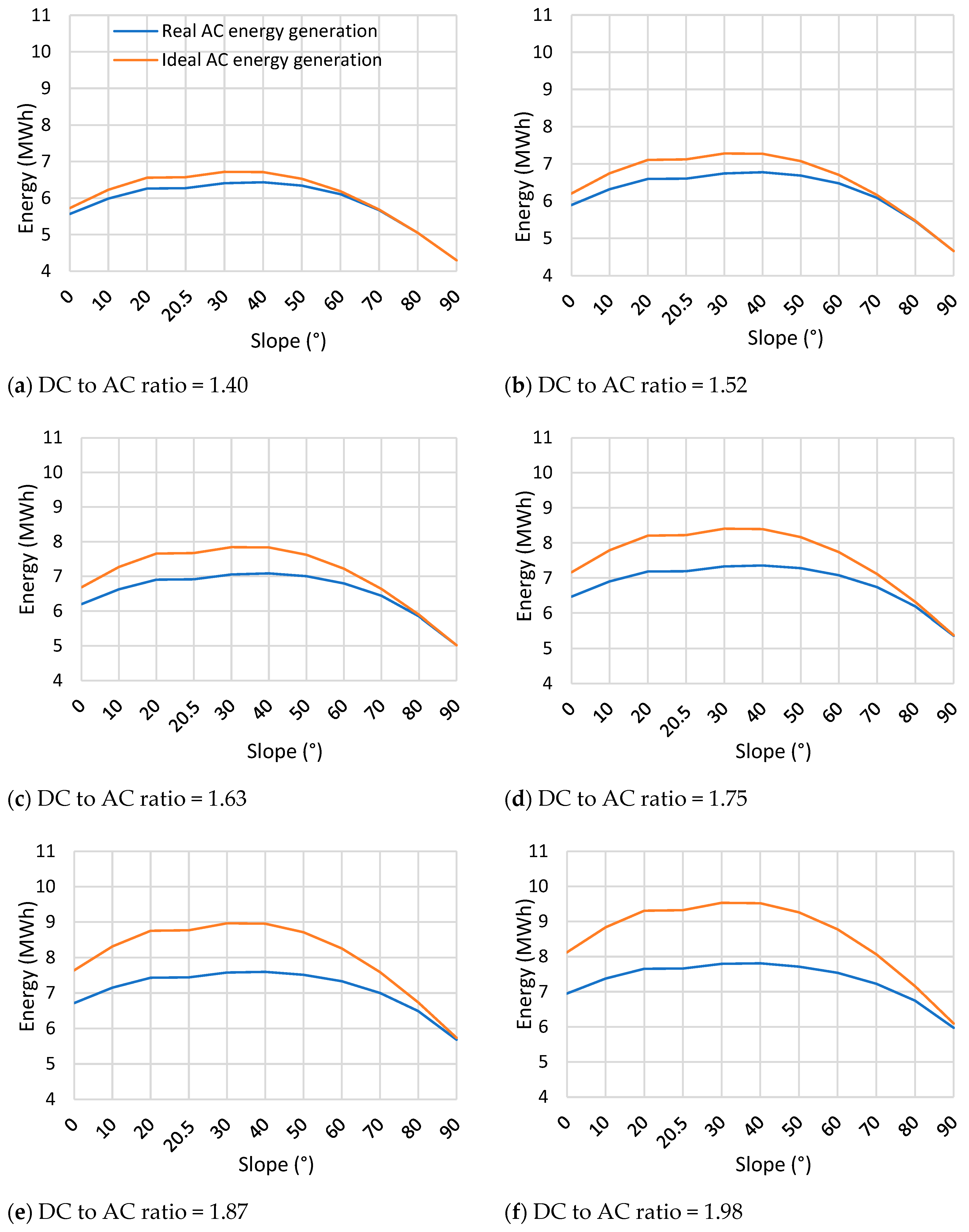
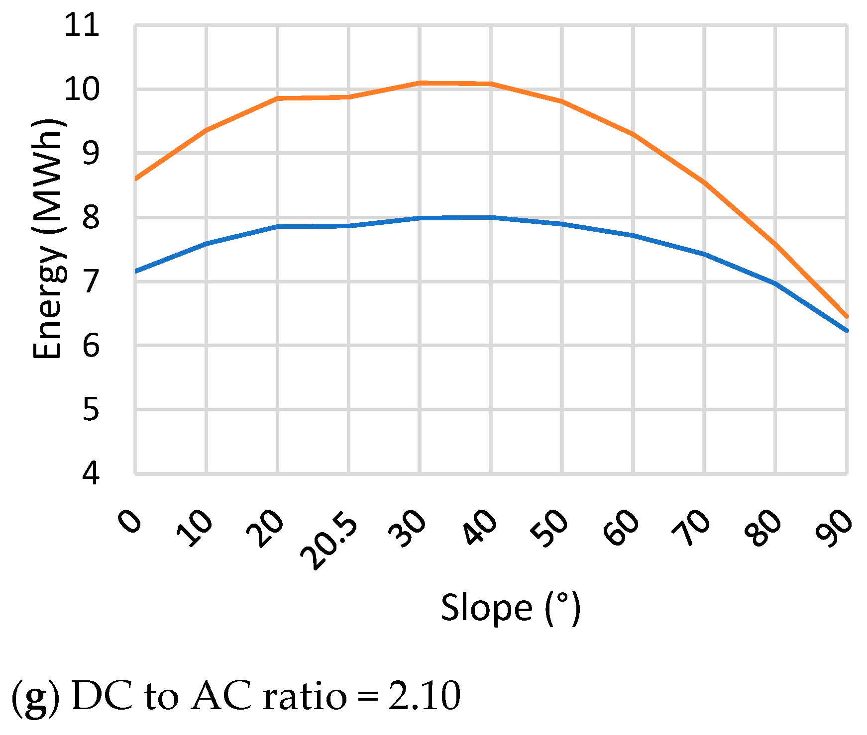
Simulations corresponding to Table 5 scenarios with a 10° step-slope from 0° to 90° for each DC to AC ratio, a fixed azimuth of 202°, and a DC to AC ratio of 1.40 were evaluated to analyse the PV system’s sensitivity against slope changes and to monitor how clipping losses are modified.

3.6.1. Energy generation

Figure 18 only shows the graphs from the DC to AC ratio of 1.40 onwards, since this is when clipping losses first became significant. As expected, it shows that as the DC to AC ratio increased, the energy production increased, negatively contributing to an increase in the inverter clipping losses. The highest clipping losses were found in acute layouts, and this was due to the latitude where the PV system was installed, which favours a greater capture of solar radiation for slopes close to 38°, while for opposite angles such as 270°, the generation of energy and its corresponding losses were much lower.

However, as already obtained, the increase in energy generation (overproduction in comparison to the base case) may not only mean an effective solution and the magnitude of the values must also be taken into account. In order to determine whether it is worth increasing the DC to AC ratio and modifying the slope, the new energy values must be compared regarding the energy overproduction and the magnitude of the effective energy from Equation (8).

Table 9. Effectiveness of the DC to AC ratio regarding energy generation for a 10° step-slope variation and a fixed slope of 202°, in kWh.

Slope	DC to AC Ratio *
	0.93	1.05	1.17	1.28	1.40	1.52	1.63	1.75	1.87	1.98	2.10
0.0°	−2157	−1679	−1208	−833	−567	−383	−264	−200	−179	−200	−258
10.0°	−1822	−1303	−816	−469	−229	−84	6	40	14	−55	−153
20.0°	−1602	−1055	−563	−224	−9	111	178	191	133	28	−114
20.5°	−1594	−1046	−554	−215	−	118	184	196	138	31	−113
30.0°	−1495	−935	−427	−83	127	238	291	283	213	83	−90
40.0°	−1502	−943	−411	−32	190	316	373	354	266	134	−47
50.0°	−1622	−1078	−541	−93	185	330	412	425	341	197	13
60.0°	−1849	−1333	−818	−327	54	283	395	445	432	330	165
70.0°	−2182	−1708	−1234	−762	−317	37	275	393	436	417	338
80.0°	−2607	−2186	−1765	−1344	−923	−522	−177	90	270	364	386
90.0°	−3105	−2746	−2387	−2028	−1669	−1311	−954	−622	−342	−119	42

* Green cells represent effective solutions, while red cells are not as effective.

varies the DC to AC ratio between 0.93 and 2.10 for slope angles between 0° and 90°, showing the results of applying Equation (8), where green cells represent effective solutions, while red cells are not as effective. It was deduced that the best solutions require a slope between 40° and 70°, and a DC to AC ratio between 1.63 and 1.87.

If one had only examined the real AC energy generation graphs from Figure 18, one would have believed that the best solution is to have a ratio of 2.1 with a slope of 20.5° as it is the solution that generated the most energy. However, it is not the best scenario compared to the base case due to the high losses it entails, energetically speaking.

Additionally, it must be noted that the results show that the slope affected power generation, but not as much as the azimuth, as can be evidenced by the significant values shown in the graphs and tables within this section.

3.6.2. Discounted Payback Period

Additionally, the economic point of view must be considered. In

Table 10. Discounted payback period (years) for a 10° step-slope variation and a fixed slope of 202°.

Slope	DC to AC Ratio *
	0.93	1.05	1.17	1.28	1.40	1.52	1.63	1.75	1.87	1.98	2.10
0.0°	8.3	8.3	8.5	8.7	9.0	9.4	9.8	10.2	10.7	11.2	11.7
10.0°	7.5	7.5	7.7	8.0	8.3	8.6	9.0	9.4	9.9	10.4	10.9
20.0°	7.1	7.1	7.3	7.6	7.9	8.2	8.6	9.0	9.5	10.0	10.5
20.5°	7.0	7.0	7.3	7.5	7.9	8.2	8.6	9.0	9.5	9.9	10.5
30.0°	6.9	6.9	7.1	7.4	7.7	8.1	8.4	8.9	9.3	9.8	10.3
40.0°	7.0	7.0	7.2	7.4	7.7	8.1	8.5	8.9	9.4	9.8	10.4
50.0°	7.2	7.2	7.5	7.6	7.9	8.3	8.7	9.1	9.6	10.1	10.6
60.0°	7.8	7.8	8.0	8.2	8.4	8.7	9.1	9.5	10.0	10.5	11.1
70.0°	8.7	8.7	9.0	9.1	9.3	9.5	9.8	10.2	10.7	11.2	11.8
80.0°	10.3	10.3	10.7	10.8	11.0	11.1	11.3	11.7	12.1	12.6	13.1
90.0°	13.2	13.2	13.6	13.9	14.1	14.3	14.5	14.7	15.0	15.4	15.9

* Green cells represent effective solutions, while red cells are not as effective.

, the DC to AC ratio is varied between 0.93 and 2.10 for slope angles between 0° and 90°, showing the results of applying Equation (10), where green cells represent good solutions, while red cells are not as good. As mentioned previously, the lower the DC to AC ratio, the lower the discounted payback period since fewer PV panels are required. In terms of slope variation, lower discounted payback periods were found between 30° and 40°, as more energy was generated due to favourable angles.

3.7. Azimuth, Slope, and DC to AC Ratio Combination

Finally, all combinations of the 30° step-azimuth, 10° step-slope variations, and the DC to AC ratio variations were studied to obtain which ranges are best for better performance in this PV installation regarding the features already mentioned.

Results show that the best option, energetically and economically speaking, is for a DC to AC ratio of 1.63, an azimuth of 180°, and a slope of 20.5°, with 6922 kWh generated and a discounted payback period of 8.6 years.

4. Discussion

Since PV panel prices have fallen lately, increasing the inverter DC to AC ratio may increase its use, which may be useful in locations without constant sun hours, that is to say, to lose some AC output energy due to inverter clipping losses is worthwhile if considering the total generated energy that the user gains. Consequently, when considering a PV project design, it would be optimal to increase the power ratio between the PV panels’ DC output power and the solar inverter’s AC output power.

In addition, increasing the DC to AC ratio may also increase the energy generation at peak hours, during higher solar irradiation values. Solar irradiation peak hours lead to a saturation of the inverter AC output energy, thus flattening the curve, usually during midday hours. Residential peak demand usually overlaps with these hours, although it may vary depending on the system load profile.

As the installation of grid-connected PV systems is increasing, the need for energy-storage systems and demand management is becoming a reality. Hence, with increasing DC to AC ratios, the overproduction of solar PV energy during peak solar hours could be increased, and this energy could be absorbed through storage and demand management.

Regarding the slope sensitivity analysis, modifying the slope angle has an effect on total annual clipping and energy generation compared to the higher results obtained in the azimuth sensitivity. PV panels angled at 30° and a DC to AC ratio of 1.40 resulted in a slight increase of 2.2% in energy generation but 3.3% in clipping losses, concerning the base case. Higher DC to AC ratios of 2.10 with the same slope angle resulted in greater energy generation of 1.56% and fewer clipping losses of 5.0%, concerning its corresponding base case. In other words, the slope variation had a positive effect on energy generation as it became closer to the latitude angle. However, concerning the effective energy due to the variation, it was most appreciated in DC to AC ratios between 1.63 and 1.87.

Regarding the azimuth sensitivity analysis, modifying the azimuth angle had an effect on total annual clipping and energy generation. PV panels with an azimuth of 180° and a DC to AC ratio of 1.40 resulted in an increase of 0.2% in energy generation but 1.3% in clipping losses, concerning the base case. Higher DC to AC ratios of 2.10 with the same azimuth angle resulted in a greater energy generation of 0.2%, but 0.4% of clipping losses concerning its corresponding base case.

There was also a seasonal effect concerning the DC to AC ratio variation. Figure 16 shows that the energy lost due to clipping was clustered in hotter months, such as April and June, and even non-existent in colder months, such as January and December, obtaining that the higher the DC to AC ratio, the higher the losses due to clipping in all periods (mainly in hotter months), noticeably affecting the annual output.

5. Conclusions

This work presented the performance of a PV residential installation. This work aimed to address the impact of the inverter DC to AC ratio, slope, and azimuth parameters when designing a solar project and calculating losses due to clipping.

The first step was the DC to AC ratio variation while keeping the azimuth and slope constant. The best ratios were found to be between 1.63 and 1.87, specifically 1.63, generating 6922 kWh per year, and a discounted payback period of 8.6 years.

The second step was the variation of the azimuth for each DC to AC ratio while keeping the slope constant. Optimum solutions varied from azimuths of 180° to 202° depending on the inverter ratio. However, also taking into account the discounted payback period, the best azimuth was found to be 180°, and a DC to AC ratio between 1.63 and 1.75.

The third step was the variation of the slope for each DC to AC ratio while keeping the azimuth constant. Optimum solutions varied from slopes of 40° to 70° (regarding the effectiveness to the base case) depending on the inverter ratio. However, also taking into account the discounted payback period, the best slopes were found to be between 40° and 50°, and a DC to AC ratio between 1.63 and 1.87.

Moreover, it was observed that increasing the ratio in solar inverters can be a good practice to obtain a higher power generation up to a certain point since there comes a limit when the clipping losses are greater than the increase in generation. In addition, this type of installation can be further improved if the solar photovoltaic installation takes into account a good setting of the slope and azimuth, especially the latter. In turn, a good setting of these three parameters will imply a reduction in the return on investment.

Finally, it has been noted that energy production increased as the DC to AC ratio increased, that clipping losses accumulated in mid-day hours, and that they increased in greater proportion as the DC to AC ratio increased, both in annual and hourly values.

Future works should study how much the PV module degradation may mitigate clipping losses over time and how it could be affected by possible disturbances in the system. In addition, a physical implementation taking into account the results obtained in this work must be considered for further validation.