Nesting Elterman Model and Spatiotemporal Linear Mixed-Effects Model to Predict the Daily Aerosol Optical Depth over the Southern Central Hebei Plain, China

Abstract

Aerosol optical depth (AOD), an important indicator of atmospheric aerosol load, characterizes the impacts of aerosol on radiation balance and atmospheric turbidity. The nesting Elterman model and a spatiotemporal linear mixed-effects (ST-LME) model, which is referred to as the ST-Elterman retrieval model (ST-ERM), was employed to improve the temporal resolution of AOD prediction. This model produces daily AOD in the Southern Central Hebei Plain (SCHP) region, China. Results show that the ST-ERM can effectively capture the variability of correlations between daily AOD and meteorological variables. After being validated against the daily Multi-Angle Implementation of Atmospheric Correction (MAIAC) AOD, the correlation coefficient between daily retrieved AOD from ST-ERM and MAIAC observations in 2017 reached 0.823. The validated Nash–Sutcliffe efficiency (E_f) of daily MAIAC AOD and ST-ERM-retrieved AOD is greater than or equal to 0.50 at 72 of the 95 stations in 2017. The relative error (E_r) is less than 14% at all the stations except for Shijiazhuang (17.5%), Fengfeng (17.8%), and Raoyang (30.1%) stations. The ST-ERM significantly outperforms the conventional meteorology–AOD prediction approaches, such as the revised Elterman retrieval model (R-ERM). Thus, the ST-ERM shows great potential for daily AOD estimation in study regions with missingness of data.

1. Introduction

Aerosol particles in the atmosphere play important roles in global and regional environments [1,2]. The aerosol optical depth (AOD), one of the key parameters characterizing the total quantity of aerosols in the atmosphere, is widely used in surface air-quality monitoring and long-term climate change prediction [3,4,5]. Thus, spatiotemporally resolved AOD characterizations are essential to improving the understanding of the impacts of aerosols on climate change and human health [6]. The AOD observations from stationary monitoring stations, such as the Aerosol Robotic Network (AERONET) [7], can provide measurements with high time resolution; however, the spatial coverage is limited [1]. Complex process-based chemical transport models are useful tools for interpreting the AOD spatiotemporal variability; however, the incomplete information on emission inventories often hampers the models’ performance [6,8]. Satellite remote sensing, such as Moderate Resolution Imaging Spectroradiometer (MODIS) AOD products [9], can provide AOD data with wide spatial coverage, but the temporal resolution is limited. Moreover, the presence of cloud contamination and bright surface generally lead to 40–80% nonrandom missingness of satellite AOD retrieval on average [8,10,11]. Therefore, producing new AOD data with wide spatial coverage and long-term sequences is essential to fill the missingness of ground and satellite-based AOD product.

AOD prediction based on meteorological variables, such as visibility from ground monitoring stations with long-term series, is another useful method [1,12,13,14,15]. This method is less disturbed by cloud cover. Moreover, meteorological stations are distributed more densely and evenly than the AOD monitoring stations mainly distributed in large- and medium-sized cities [16]. This scenario provides great potential for retrieving AOD with high spatial and temporal resolution using visibility-dominated surface meteorological variables. Early studies estimated the AOD using a simple linear regression method by considering visibility as an independent variable [17,18,19,20,21]. These studies mostly retrieve daily mean or early afternoon visibility as AOD by assuming an exponential decline of aerosol particle concentration with altitude [18,22]. Given the spatial variability of aerosol particle concentration attenuation with height, a water vapor pressure parameter was introduced into the visibility-based AOD prediction model to correct the vertical profile of aerosol extinction [23]. Moreover, the nonlinear least squares method was used for modifying the model parameters of each site to make the visibility-based AOD prediction method suitable for different regional geographical environments; the high-accuracy M-Elterman [14] and KM-Elterman [24] models were also proposed. However, the models using the nonlinear least squares method are hampered by inaccurate empirical parameters, thereby strongly affecting the models’ universality. Thus, Wu et al. [1] addressed the model’s inaccurate parameters by introducing the particle swarm optimization (PSO) algorithm into the M-Elterman model to develop the PSO-M-Elterman model, which prominently improved AOD’s available rate and accuracy. However, these studies consider visibility the only controlling element of aerosol scale height (ASH), leading to the overestimation and underestimation of the AOD in winter and summer, respectively. Given the relevance of ASH in AOD prediction, Li et al. [2] investigated the impacts of meteorological variables on ASH. Furthermore, they revised the ASH calculation method to develop the revised Elterman retrieval model (R-ERM); thus, the estimation accuracy of AOD was considerably improved. The above models’ estimates have proven to be precise on monthly, quarterly, and annual time scales. However, the deterministic models of the studies mentioned cannot easily capture exactly the strongly spatiotemporal variability of the AOD–meteorological factor relationship at the daily time scale because of the regional variability in the emission intensity of aerosol particles, aerosol chemical composition, and atmospheric diffusion conditions. This scenario is unfavorable to building an AOD product with high spatiotemporal resolution. Given the spatiotemporal heterogeneities of different predictors, the spatiotemporal linear mixed-effects (ST-LME) model is often employed to solve complex nonlinearity problems [25]. The approach can be used to improve the meteorological variable-based AOD prediction method.

China has a dense network of meteorological monitoring stations, including 2450 national meteorological stations and more than 60,000 regional stations [16]. The abundant meteorological materials observed from these stations contribute to the retrieval of AOD with high spatiotemporal resolution. In this study, a ST-LME model is presented to improve the Elterman retrieval model (ERM). The improved model, named the ST-ERM, uses meteorological variables to retrieve the AOD in Southern Central Hebei Plain (SCHP), China. The meteorological variable data and the MAIAC AODs with 1 km spatial resolution in 2016 were employed to develop the ST-ERM. The MAIAC AOD in 2017 was used to validate the model’s applicability. We calculated the daily AOD over the study area utilizing the ST-ERM and further depicted the spatiotemporal variation of the seasonal and annual average AOD. Furthermore, the AOD estimations of the ST-ERM were compared with those of the R-ERM from Li et al. [2] to assess the ST-ERM performance well. This study will enrich the method of the AOD prediction model and further provide support for the AOD inversion with long-term application and a wide range in other regions.

2. Dataset and Methodologies

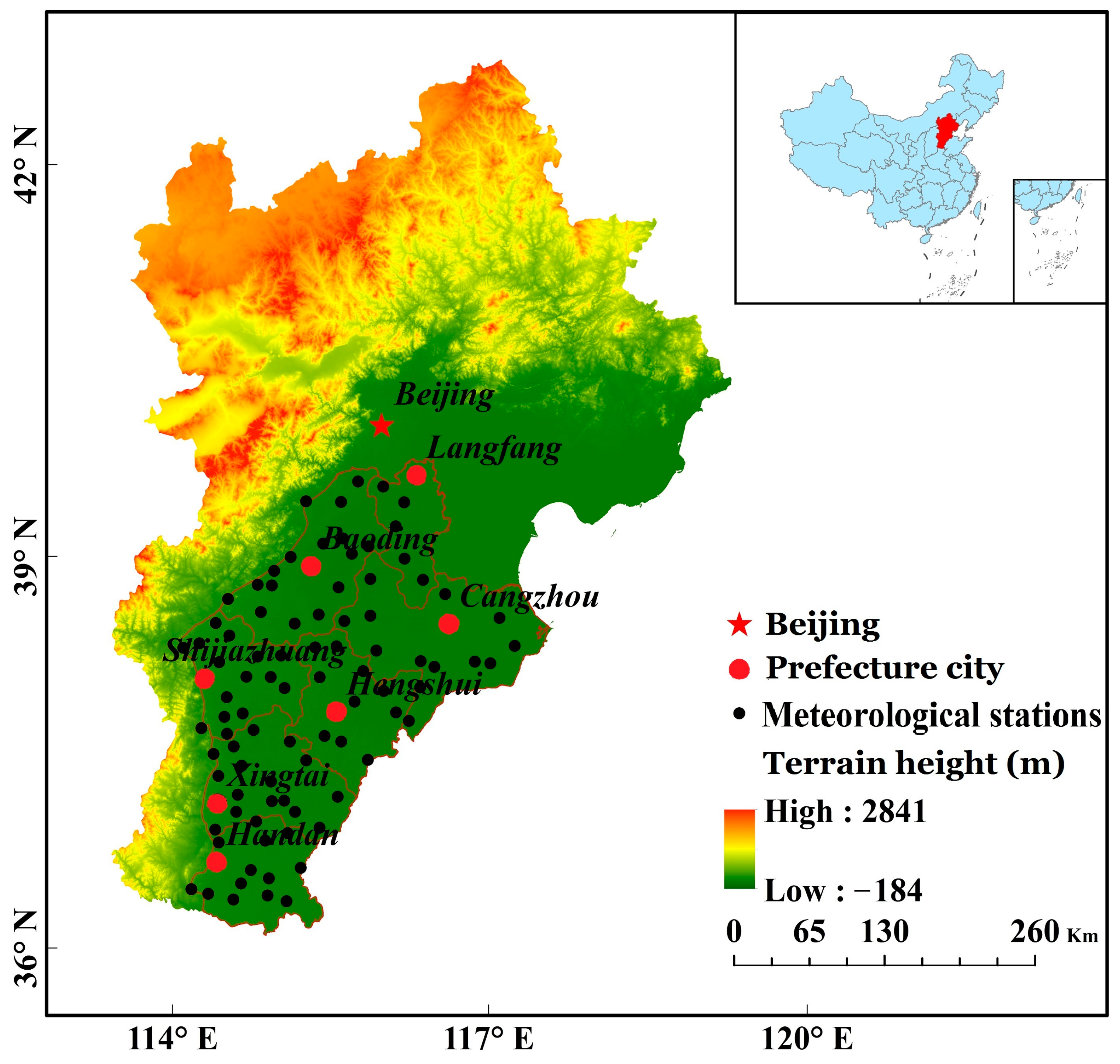
2.1. Study Area

The study area is the SCHP, which is the major industrial and agricultural production base of Hebei Province, located in the hinterland of the North China Plain. The research area covers Cangzhou and Hengshui and some areas of Shijiazhuang, Handan, Xingtai, Baoding, and Langfang with an area of 62,800 km², including a population of more than 50 million [2], as shown in Figure 1. During the past 40 years, the urbanization and industrialization in the SCHP region developed rapidly; a large number of air pollutants have been also produced during this time [26]. In addition, the SCHP region is located in the piedmont areas of the Taihang Mountains and Yanshan Mountains. These areas are unfavorable to pollutant diffusion. Moreover, these factors contributed to making the SCHP region one of the most seriously polluted regions in the world [2,27].

2.2. Dataset

2.2.1. Meteorological Variables and Elevation Data

In this study, hourly meteorological variable observations of 95 stations in the SCHP region from 2016 to 2017 were downloaded from the China Meteorological Data Sharing Service System (http://data.cma.cn/ (accessed on 26 October 2021)). The meteorological variables with a 6 h temporal resolution, including atmospheric pressure (P), air temperature (T), ground horizontal visibility (V), water vapor pressure (VP), wind speed (W), and relative humidity (RH), were monitored at 2:00, 8:00, 14:00, and 20:00 Beijing time. However, the ground horizontal visibility observed at 2:00, 8:00, and 20:00 was susceptible to radiation fog, light, and surface inversion, which could cause biases. Thus, the meteorological data at 14:00 of each day were employed in the present study to estimate the AOD. Moreover, screening for meteorological data was necessary because of the extreme weather influence. Therefore, weather data for weather conditions, such as high humidity (RH > 90%), precipitation above 2.5 mm, and snow, were removed [14].

The digital elevation model (DEM) materials were collected by the National Aeronautics and Space Administration (NASA) Shuttle Radar Topographic Mission (SRTM). The data, which have a spatial resolution of approximately 90 m, can be obtained from the Consortium for Spatial Information of the United States Geological Survey (http://srtm.csi.cgiar.org/srtmdata/ (accessed on 4 September 2021)).

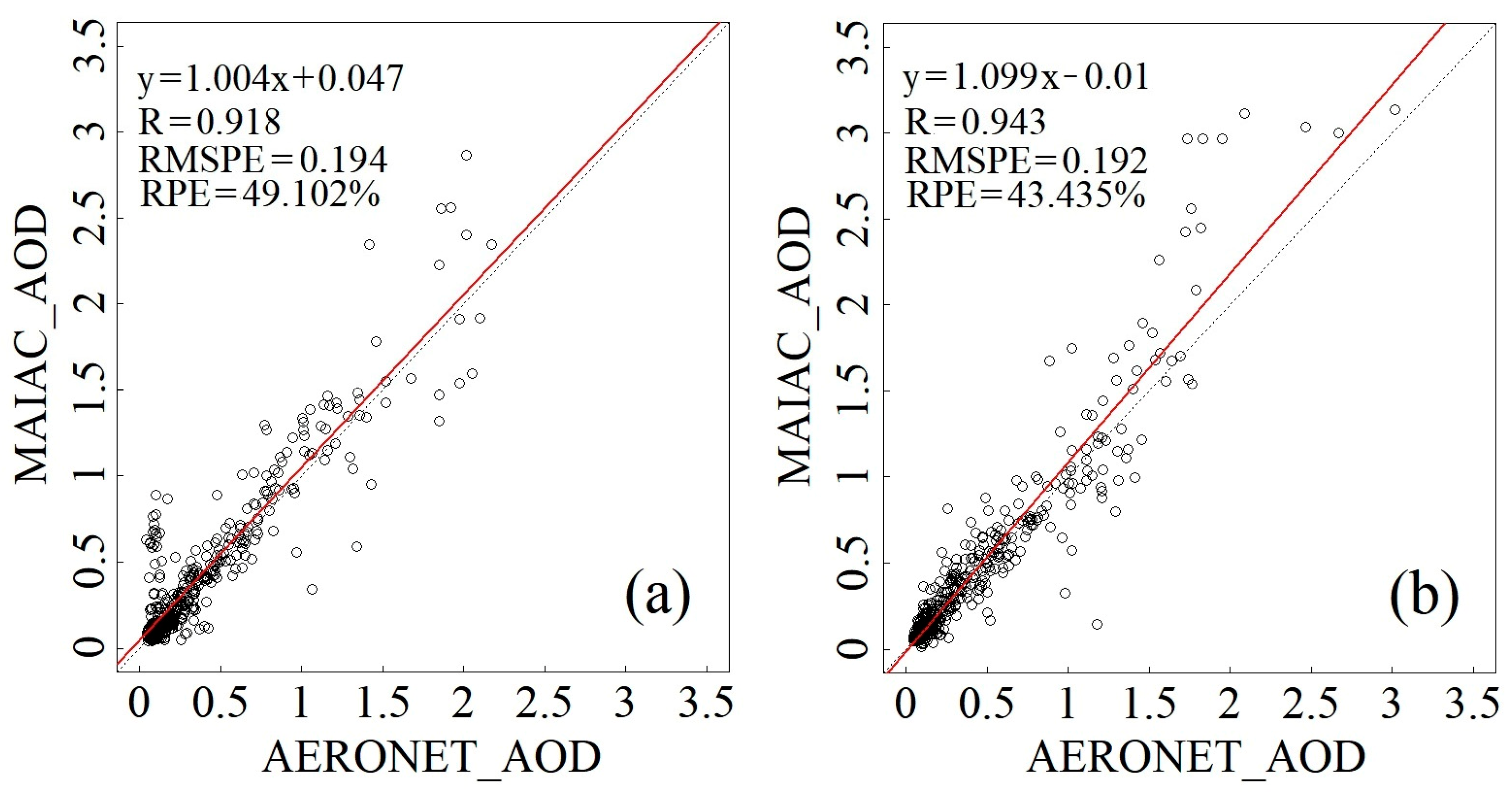
2.2.2. Multi-Angle Implementation of Atmospheric Correction (MAIAC) AOD

The MAIAC from the Aqua and Terra MODIS, passing over at 1:30 p.m. and 10:30 a.m. local time, respectively, is a new generic algorithm to retrieve the AOD and atmospheric correction [28]. It can dynamically collect the surface reflection relationship of the MODIS blue and shortwave infrared bands over the dark and bright regions using the time series method to improve the data accuracy and spatial resolution considerably [29,30]. The MAIAC AOD products with 1 km spatial resolution perform better than the MODIS 3 and 10 km products over China [31]. The daily MAIAC AOD was collected from the NASA Center for Climate Simulation (ftp://[email protected]/DataRelease/ (accessed on 26 October 2021)). In the present study, we extracted the AOD values at 550 nm from 2016 to 2017. Moreover, the Aqua MAIAC AOD product at 1:30 p.m. was employed to match with the sampling time of meteorological variables. In consideration of the random missingness of AOD products from Aqua, monthly simple linear regression models using the least squares method were fitted to obtain the correlation between Terra and Aqua AODs (

Table 1. The monthly correlations between the AODs with 1 km spatial resolution from Aqua and Terra.

Months	Correlations-R
	2016	2017
1	0.90	0.93
2	0.84	0.93
3	0.94	0.91
4	0.91	0.92
5	0.92	0.96
6	0.92	0.84
7	0.83	0.90
8	0.88	0.85
9	0.93	0.89
10	0.92	0.84
11	0.87	0.87
12	0.90	0.91
Annual average	0.90	0.90

). Moreover, the models were employed to calculate the AOD missingness from Aqua using the available AOD from Terra [2,32]. In the present study, the MAIAC AOD data during the periods of 2016 and 2017 were employed to construct and validate the model, respectively.

The AERONET AOD, which can provide in AOD measurements via sun photometers, has been widely used to validate AOD prediction [33,34]. In the present study, the AERONET AOD observations (level 2, version 3) from the Beijing-CAMS, Beijing, and Xianghe sites were applied to evaluate the availability of MAIAC AOD. Following the wavelength of MAIAC AOD, AERONET AOD at 550 nm was calculated by interpolating AOD at 440 and 675 nm using the reported angstrom exponents for respective wavelengths [2]. The AERONET AOD measurements within the temporal window of ±30 min on the MODIS overpass time were collected and averaged to match the MAIAC AOD products covering the AERONET site. The correlations between the AERONET AOD and MAIAC AOD in 2016 (a) and 2017 (b) are shown in Figure 2. The results demonstrate that MAIAC AOD shows significant correlation with the AERONET AOD. Moreover, the correlations between MAIAC AOD and AERONET AOD had values of 0.918 and 0.943 for 2016 and 2017, respectively. In addition, the root-mean-square prediction error (RMSPE) and slope ranged from 0.192 to 0.194 and 1.004 to 1.099, respectively.

2.2.3. Data Integration

Following the spatial resolution of MAIAC AOD (1 km), the DEM (90 m) was resampled into the grid DEM with the same spatial resolution (1 km) in ArcGIS (Version 10.2; ESRI). Then, the meteorological variables were matched with the corresponding grid cells of AOD and DEM covering the monitoring stations. Finally, we obtained 10,949 and 13,427 matched samples for 2016 and 2017, respectively.

2.3. Methodologies

2.3.1. Retrieval Method

Following Koschmieder’s law [19], the meteorological visibility (V) can be obtained by the extinction coefficient e₀.₅₅ in the 550 nm wavelength according to the following expression:

V = 3.912/e_0.55.

(1)

Aerosols are assumed to obey a Junge distribution in standard cases, i.e., n(r) = cr^−(v*+1), where c is a constant, r is the particle radius, and v* = 3 does not change with height. Under the standard atmospheric conditions with 15 °C of surface air temperature and 1013 hPa of pressure, the aerosol extinction coefficient at λ wavelength at height z can be expressed as

$${\mathrm{e}}_{\mathsf{\lambda }}=\frac{{\mathrm{N}}_{\mathrm{a}}\left(\mathrm{z}\right)}{{\mathrm{N}}_{\mathrm{a}}\left(0\right)}\left(\frac{3.912}{\mathrm{V}}-0.0116\right){\left(\frac{0.55}{\mathsf{\lambda }}\right)}^{{\mathrm{v}}^{*}-2},$$

(2)

where ${\mathrm{N}}_{\mathrm{a}}\left(0\right)$ and ${\mathrm{N}}_{\mathrm{a}}\left(\mathrm{z}\right)$ are the concentrations of aerosol particles at the surface and height Z, respectively.

McClatchey et al. [35] reported the following aerosol particle concentration height profile:

$${\mathrm{N}}_{\mathrm{a}}\left(\mathrm{z}\right)\{\begin{array}{c}55\exp \left[-\frac{\left(\mathrm{z}-5.5\right)}{{\mathrm{ASH}}_1}\right]\left(\mathrm{z}\le 5.5 \mathrm{km}\right)\\ 55 \left(5.5\le \mathrm{z}\le 18 \mathrm{km}\right)\\ 55\exp \left(-\frac{\left(\mathrm{z}-18\right)}{{\mathrm{ASH}}_2}\right)(\mathrm{z}>18 \mathrm{km})\end{array},$$

(3)

where ASH₁ = 0.886 + 0.0222 V (km), and ASH₂ = 3.77 km.

Elterman [18] established the relational expression between the visibility at the corrected sea level (i.e., V) and the visibility observed by the meteorological station at the altitude Z (i.e., V_z) by using the distribution of aerosol particle concentrations with height developed by McClatchey et al. [35]:

$${\mathrm{V}}_{\mathrm{z}}=\frac{3.912}{0.0116-0.00099\mathrm{Z}+\left(\frac{3.912}{\mathrm{V}}-0.0116\right){\mathrm{e}}^{-\frac{\mathrm{Z}}{\left(0.886+0.0222\mathrm{V}\right)}}}$$

(4)

Thus, the atmospheric aerosol optical thickness AOD is deduced as

$$\mathrm{AOD}=\left(\frac{3.912}{\mathrm{V}}-0.0116\right){\left(\frac{0.55}{\mathsf{\lambda }}\right)}^{{\mathrm{v}}^{*}-2}\left[{\mathrm{ASH}}_1\left({\mathrm{e}}^{-\frac{\mathrm{z}}{{\mathrm{ASH}}_1}}-{\mathrm{e}}^{-\frac{5.5}{{\mathrm{ASH}}_1}}\right)+12.5{\mathrm{e}}^{-\frac{5.5}{{\mathrm{ASH}}_1}}+{\mathrm{ASH}}_2{\mathrm{e}}^{-\frac{5.5}{{\mathrm{ASH}}_1}}\right].$$

(5)

The above approach is the conventional ERM for retrieving the AOD. In this model, atmospheric visibility is the only control factor of ASH₁.

Given the spatial heterogeneity of aerosol height profile for different regions and the impacts of other factors on the ASH₁, such as water vapor, the ERM may bring biases to the AOD prediction results [36]. Thus, Qiu and Lin [37] introduced a correction factor φ into the ERM to develop further a revised retrieval model suitable for the China region:

$$\mathrm{AOD}=\left(\frac{3.912}{\mathrm{V}}-0.0116\right){\left(\frac{0.55}{\mathsf{\lambda }}\right)}^{{\mathrm{v}}^{*}-2}\left[{\mathrm{ASH}}_1\left({\mathrm{e}}^{-\frac{\mathrm{z}}{{\mathrm{ASH}}_1}}-{\mathrm{e}}^{-\frac{5.5}{{\mathrm{ASH}}_1}}\right)+12.5{\mathrm{e}}^{-\frac{5.5}{{\mathrm{ASH}}_1}}+{\mathrm{ASH}}_2{\mathrm{e}}^{-\frac{5.5}{{\mathrm{ASH}}_1}}\right]\mathsf{\phi },$$

(6)

where φ has two expressions in the China region. In Northeast China, the φ is expressed as

$$\mathsf{\phi }={\mathrm{e}}^{-0.32+0.02\mathrm{Vz}}.$$

(7)

For the regions outside of Northeast China,

$$\mathsf{\phi }={\mathrm{e}}^{\left(0.42+0.0046{\mathrm{p}}_{\mathrm{w}}+0.015\mathrm{Vz}\right)\exp \left(-0.0047{\mathrm{V}}_{\mathrm{z}}^2/{\mathrm{p}}_{\mathrm{w}}\right)},$$

(8)

where p_w denotes the water vapor pressure (hPa).

Equations (6)–(8) formed the QRM, which improves the accuracy of the AOD prediction utilizing the meteorological variables [14]. Although the ASH₁ estimation is the key parameter for AOD prediction, its estimation in ERM and QRM depends only on atmospheric visibility; hence, biases may be introduced into the AOD estimation [2].

Therefore, Li et al. [12] further revised the ASH₁ empirical model as follows:

$${\mathrm{ASH}}_1={\mathrm{e}}^{\left(0.023 \mathrm{V}+0.031{\mathrm{P}}_{\mathrm{w}}-0.402\right)}.$$

(9)

Finally, the model is further incorporated into Equation (6) to develop the R-ERM:

$$\mathrm{AOD}=\left(\frac{3.912}{\mathrm{V}}-0.0116\right)\frac{0.55}{\mathsf{\lambda }}\ast \left[{\mathrm{ASH}}_1\left(\mathrm{V},{\mathrm{P}}_{\mathrm{w}}\right)\left({\mathrm{e}}^{-\frac{\mathrm{Z}}{{\mathrm{ASH}}_1\left(\mathrm{V},{\mathrm{P}}_{\mathrm{w}}\right)}}-{\mathrm{e}}^{-\frac{5.5}{{\mathrm{ASH}}_1\left(\mathrm{V},{\mathrm{P}}_{\mathrm{w}}\right)}}\right)+12.5{\mathrm{e}}^{-\frac{5.5}{{\mathrm{ASH}}_1{\left(\mathrm{V},{\mathrm{P}}_{\mathrm{w}}\right)}_1}}+{\mathrm{ASH}}_2{\mathrm{e}}^{-\frac{5.5}{{\mathrm{ASH}}_1\left(\mathrm{V},{\mathrm{P}}_{\mathrm{w}}\right)}}\right].$$

(10)

Eventually, the AOD can be retrieved using Equation (10).

In the present study, the ASH₁ algorithm was further revised using ST-LME to improve the performance of the AOD prediction model further. Then, the improved ASH₁ estimation model was introduced into the ERM to develop the ST-ERM.

The ST-LME model, including the information’s fixed and random effects can effectively capture the spatiotemporal variability in local effects [38]. Based on the temporal random effect of the LME model, the spatial random effect was employed to correct the spatiotemporal heterogeneity of the relationship between ASH₁ and its influence factors. Therefore, the ST-LME model can characterize the spatiotemporal characteristics of the relationship between ASH₁ and its influence factors in the SCHP region. In the present study, the ST-LME model was selected to reflect the correlation and heterogeneity between the data to correct the ASH₁ further. The specific model is expressed as follows:

$$\begin{gathered} {\mathrm{ST}}_{\mathrm{ASH}1}=\left(\mathsf{\alpha }+{\mathrm{u}}_{\mathrm{t}1}+{\mathrm{u}}_{\mathrm{t}2}\right)+\left({\mathsf{\beta }}_1+{\mathrm{v}}_{\mathrm{t}1}+{\mathrm{v}}_{\mathrm{t}2}\right){\mathrm{VP}}_{\mathrm{st}}+\left({\mathsf{\beta }}_2+{\mathrm{k}}_{\mathrm{t}1}+{\mathrm{k}}_{\mathrm{t}2}\right){\mathrm{RH}}_{\mathrm{st}}+ \\ \left({\mathsf{\beta }}_3+{\mathrm{m}}_{\mathrm{t}1}+{\mathrm{m}}_{\mathrm{t}2}\right){\mathrm{T}}_{\mathrm{st}}+\left({\mathsf{\beta }}_4+{\mathrm{h}}_{\mathrm{t}1}+{\mathrm{h}}_{\mathrm{t}2}\right){\mathrm{V}}_{\mathrm{st}}+\left({\mathsf{\beta }}_5+{\mathrm{w}}_{\mathrm{t}1}+{\mathrm{w}}_{\mathrm{t}2}\right){\mathrm{P}}_{\mathrm{st}}+ \\ \left({\mathsf{\beta }}_6+{\mathrm{e}}_{\mathrm{t}2}\right){\mathrm{DEM}}_{\mathrm{st}}+\left({\mathsf{\beta }}_7+{\mathrm{n}}_{\mathrm{t}1}+{\mathrm{n}}_{\mathrm{t}2}\right){\mathrm{W}}_{\mathrm{st}}+{\mathsf{\epsilon }}_{\mathrm{st}}\left({\mathrm{u}}_{\mathrm{t}1}{\mathrm{v}}_{\mathrm{t}1}{\mathrm{k}}_{\mathrm{t}1}{\mathrm{m}}_{\mathrm{t}1}{\mathrm{h}}_{\mathrm{t}1}{\mathrm{w}}_{\mathrm{t}1}{\mathrm{n}}_{\mathrm{t}1}{\mathrm{p}}_{\mathrm{t}1}\right)~ \\ \mathrm{N}\left(0,\sum \right),\left({\mathrm{u}}_{\mathrm{t}2}{\mathrm{v}}_{\mathrm{t}2}{\mathrm{k}}_{\mathrm{t}2}{\mathrm{m}}_{\mathrm{t}2}{\mathrm{h}}_{\mathrm{t}2}{\mathrm{w}}_{\mathrm{t}2}{\mathrm{e}}_{\mathrm{t}2}{\mathrm{n}}_{\mathrm{t}2}{\mathrm{p}}_{\mathrm{t}2}\right)~ \mathrm{N}(0,\sum ),{\mathsf{\epsilon }}_{\mathrm{st}}~\mathrm{N}\left(0,{\mathsf{\sigma }}^2\right) \end{gathered}$$

(11)

where ${\mathrm{ST}}_{\mathrm{ASH}1}$ is the daily ASH₁ calculated from the MAIAC AOD using ERM at s meteorological station on day t, which is considered the observed ASH₁ in this study; VP, RH, T, V, P, W, and DEM are vapor pressure, relative humidity, temperature, surface visibility, surface pressure, wind speed, and altitude, respectively; α, u_t1, and u_t2 denote the fixed and random intercept values; β₁, β₂, β₃, β₄, β₅, β₆, and β₇ are the fixed slopes of VP, RH, T, V, P, W, and DEM; U_t1, v_t1, k_t1, m_t1, h_t1, w_t1, and n_t1 denote the daily random slopes of each meteorological variable; u_t2, v_t2, k_t2, m_t2, h_t2, w_t2, e_t2, and n_t2 are the site random effect slopes of each meteorological variable; and ${\mathsf{\epsilon }}_{\mathrm{st}}$ denotes the random error at meteorological station s on day t, and it obeys independent equal variance multivariate normal distribution. Each random effect also obeys multivariate normal distribution, where Σ is the unstructured variance–covariance matrix of random effect.

The AOD estimated by the ST-ERM (hereinafter referred to as ST-AOD) was eventually compared with AODs estimated by the R-ERM (hereinafter referred to as R-AOD).

2.3.2. Model Validation

Various statistical indicators (i.e., coefficient of determination [R], RMSPE, and RPE) were calculated for observed and calculated values to assess the goodness of the model fitting. In addition, a 10-fold cross-validation (CV) approach was adopted to evaluate the performance of the method. The whole dataset for model-fitting was randomly divided into 10 subsets. Each subset approximately contained 10% of the overall dataset. For each time, one subset was chosen as the test sample, and the remaining nine subsets were combined as the training sample to fit the model. This process was repeated 10 times to guarantee that all the subsets were tested. The agreement between the observed and estimated values was assessed utilizing the R, slope, RMSPE, and RPE. The model fitting and CV statistics were compared to evaluate the degree of potential overfitting of the model.

$$\mathrm{RMSPE}=\sqrt{{\sum }_{\mathrm{i}=1}^{\mathrm{n}}{\left({\mathrm{y}}_{\mathrm{obs},\mathrm{i}}-{\mathrm{y}}_{\mathrm{model},\mathrm{i}}\right)}^2/\mathrm{n}},$$

(12)

$$\mathrm{RPE}=\frac{\mathrm{RMSE}}{\overline{\mathrm{y}}}\times 100\%,$$

(13)

where ${\mathrm{y}}_{\mathrm{obs},\mathrm{i}}$ denotes the predicted ASH₁ at $\mathrm{site} \mathrm{i}$, ${\mathrm{y}}_{\mathrm{model},\mathrm{i}}$ denotes the observed ASH₁ at $\mathrm{site} \mathrm{i}$, n denotes the total number of data samples, and $\overline{\mathrm{y}}$ denotes the mean value of the observed ASH₁.

In addition, Nash–Sutcliffe efficiency (E_f) and the relative error (E_r) were used in this study to evaluate further the estimation performance of the AOD prediction compared with that of the MAIAC AOD. E_f is usually employed to validate the goodness of prediction for the model. The value of E_f ranges from negative infinity to 1, and E_f is close to 1, indicating good model quality and high model reliability. E_f is close to 0, indicating that the simulation result is close to the average value of the observed value; that is, the overall result is credible, but the process simulation error is large. If E_f is much less than 0, the model cannot be trusted.

The variables E_f and E_r (%) were calculated as

$${\mathrm{E}}_{\mathrm{f}}=1-\frac{\sum {\left({\mathrm{Q}}_{\mathrm{obs}}^{\mathrm{t}}-{\mathrm{Q}}_{\mathrm{model}}^{\mathrm{t}}\right)}^2}{\sum {\left({\mathrm{Q}}_{\mathrm{obs}}^{\mathrm{t}}-\overline{{\mathrm{Q}}_{\mathrm{obs}}}\right)}^2},$$

(14)

$${\mathrm{E}}_{\mathrm{r}}=\left(\frac{\overline{{\mathrm{Q}}_{\mathrm{obs}}}-\overline{{\mathrm{Q}}_{\mathrm{model}}}}{\overline{{\mathrm{Q}}_{\mathrm{model}}}}\right)\times 100\%,$$

(15)

where ${\mathrm{Q}}_{\mathrm{obs}}^{\mathrm{t}}$ and ${\mathrm{Q}}_{\mathrm{model}}^{\mathrm{t}}$ are the observed and estimated AODs in daily t, and $\overline{{\mathrm{Q}}_{\mathrm{model}}}$ and $\overline{{\mathrm{Q}}_{\mathrm{obs}}}$ are the estimated and observed daily mean AOD values, respectively.

3. Results

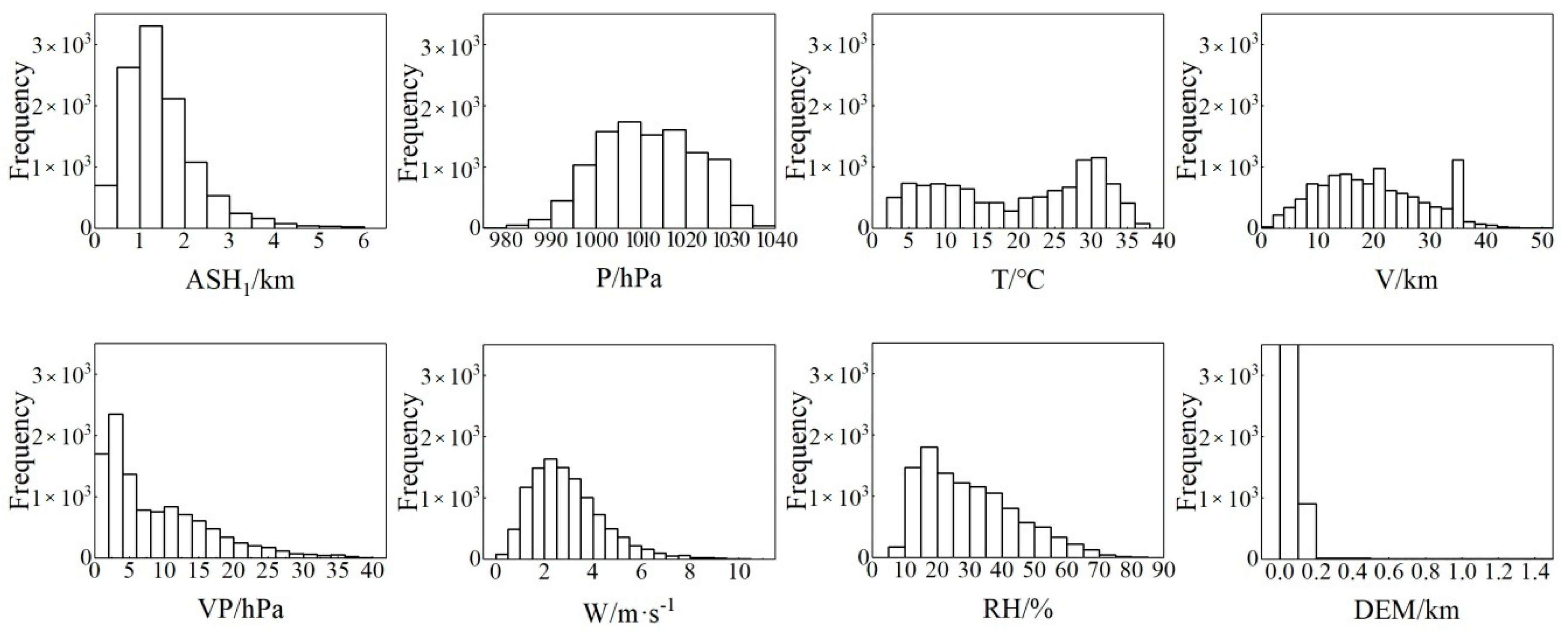
3.1. Descriptive Statistics of ST-LME

The histograms of variables, including ASH₁, DEM, and meteorological elements from the 10,949 matched samples, are shown in Figure 3. The samples were used to fit the ST-LME model for all the days in 2016. The statistical parameters, including mean, minimum, maximum value, and standard deviation for all the variables, are presented in

Table 2. Descriptive statistics of each parameter of the modeling data in 2016.

Variables	Mean	Minimum	Maximum	Std. Deviation
ASH1/km	1.475	0.058	5.995	0.842
P/hPa	1011.690	976.500	1037.300	11.030
T/°C	19.822	2.200	38	10.217
V/km	19.944	0.600	50	9.539
VP/hPa	8.755	0.600	40.700	7.513
W/m·s−¹	2.898	0	11.200	1.517
RH	0.297	0.050	0.890	0.147
DEM/km	0.046	0.004	1.454	0.085

. The variables are approximately normally distributed except for the surface air temperature (Figure 3). The mean ASH₁ is 1.475 ± 0.842 km (mean value ± standard deviation). The variables of the model’s fitting dataset indicate considerable seasonal variability. For instance, the high ASH₁ mostly exists in summer, whereas the lowest value mainly exists in spring. The meteorological variables, such as atmospheric visibility (V), also show similar variations. The spatiotemporal heterogeneity of the relationship between ASH₁ and meteorological and geographic variables is mainly due to their complex correlation caused by the spatiotemporal heterogeneity of various factors, such as atmospheric pollutant emission intensity, particulate matter composition, atmospheric diffusion conditions, and landform.

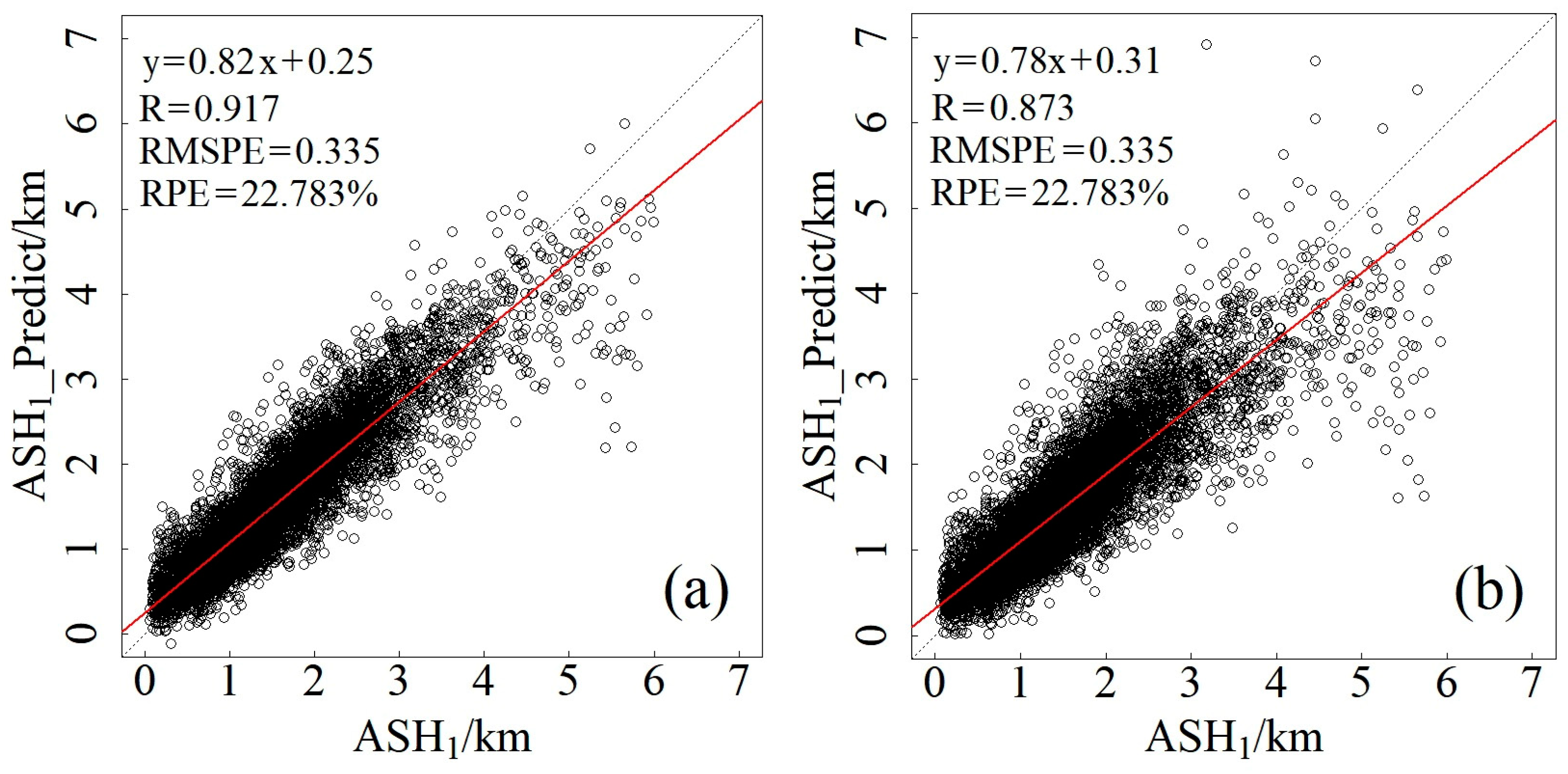
3.2. ST-LME Model Fitting and Validation

Figure 4 demonstrates the scatter plots of the ST-LME model fitting and the 10-fold CV for the SCHP region in 2016. The overall R of the model fitting is 0.917 (Figure 4a). This finding indicates that the ST-LME model can effectively interpret 84.0% of the ASH₁ variability. The fitting results also indicate that the overall RMSPE and RPE values were 0.335 and 22.783% (Figure 4a), respectively. In addition, the slope is 0.82, indicating that the prediction bias of the ST-LME model is very small. These findings demonstrate that the ST-LME model performs well.

In comparison to the model-fitting results, results of 10-fold CV show that the overall R value of 0.873 decreases by 0.044, whereas the overall RMSPE and RPE values of 0.410 and 27.836% increase by 0.075 and 5.053%, respectively. The slope value of 0.78 is also smaller than that of model fitting (Figure 4b). Thus, the CV results demonstrate that slight overfitting exists in the ST-LME model. However, the model still shows high retrieval accuracy of ASH₁.

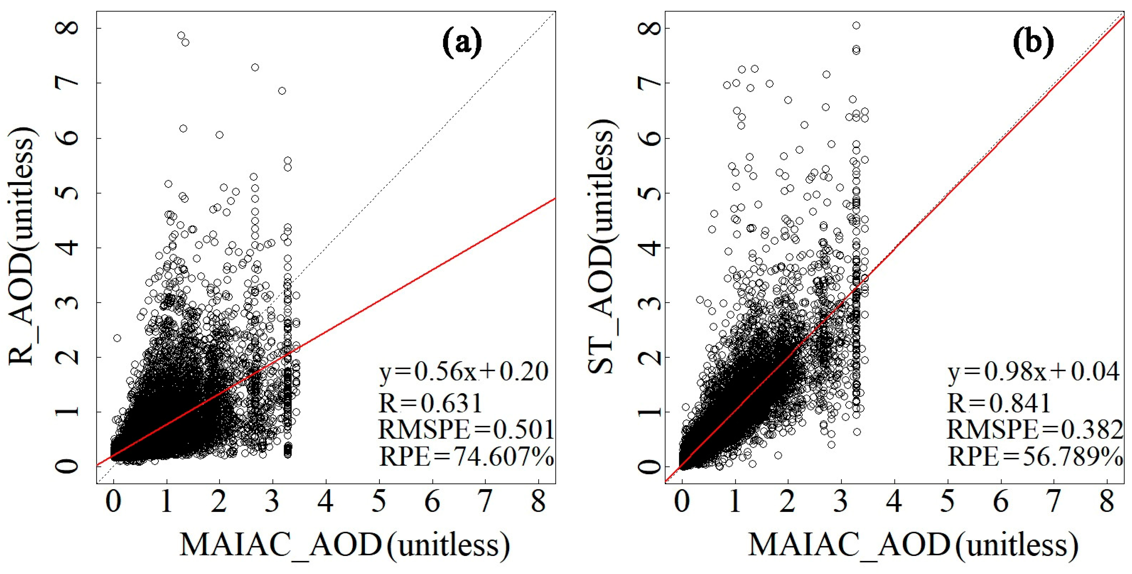
3.3. Comparisons of AOD Prediction by ST-ERM with the R-ERM

The conventional R-ERM from Li et al. [12] was also fitted using the same variable data as those employed in the ST-ERM to reveal further the impacts of the improved ASH₁ algorithm on the ST-ERM performance improvement. The daily retrieved AOD results by these models and MAIAC AOD are compared in Figure 5.

High-humidity weather strongly affects the vertical distribution of aerosol extinction. Thus, the ASH₁ deterministic algorithm in the R-ERM was developed by introducing the water vapor pressure closely related to the temperature and relative humidity into ASH₁ algorithm in Elterman model. Compared to the conventional Elterman model, the R-ERM significantly improved the accuracy of AOD prediction [2]. The correlation value between daily AOD retrieved from the R-ERM and MAIAC AOD is 0.631, and the RMSPE and RPE values are 0.501 and 74.607% (Figure 5a). In contrast, the ST-LME model was employed to develop the ASH₁ algorithm in the ST-ERM, which can effectively capture the spatiotemporal heterogeneity relationship between ASH₁ and its influence factors. By contrast, the ST-ERM considerably outperforms the R-ERM. Figure 5b shows the good results achieved by the ST-ERM, with the larger R value of 0.841 and the smaller RMSPE and RPE values of 0.382 and 56.789%, respectively. In addition, the slope value of 0.98 for the ST-ERM, which is much higher than the slope value of 0.56 for the R-ERM, demonstrates a slight prediction deviation. These findings indicate that the improved ASH₁ parameter algorithm plays an important role in AOD prediction in the ST-ERM.

In addition, compared with the ST-ERM, deterministic models, such as the R-ERM, have another flaw. In particular, the performance of these models is overly reliant on the likelihood estimation of event probability. Thus, accurately describing the quantitative parameter inversion problem is difficult.

To further assess the performance of the ST-ERM, two metrics were employed in the present study: (1) E_f represents the simulation skill of retrieved daily AOD by the ST-ERM as compared with the MAIAC observations, and (2) E_r characterizes the error in daily retrieved AOD for the study period.

Figure 6 shows the E_f and E_r between daily MAIAC AOD and retrieved AOD by the R-ERM (a–b) and ST-ERM (c–d) models in 2016. The E_f of the daily AOD between the ST-ERM estimation and the MAIAC observation is greater than or equal to 0.50 at 75 of 95 stations (Figure 6c). This finding demonstrates that the ST-ERM performs well in retrieving the AOD. By contrast, the E_f between the daily MAIAC AOD and R-ERM estimations is greater than or equal to 0.50 at 20 of 95 stations (Figure 6a), suggesting that the R-ERM has relatively poor performance for AOD prediction at the daily time scale. Our results also show that the E_f values for the R-ERM and ST-ERM all present high-in-north and low-in-south spatial patterns over the SCHP region. In addition, the E_r of daily MAIAC AOD and ST-ERM estimation is less than 18% at all the stations, except for Raoyang (27.64%) and Yongqing (19.5%). The stations with large E_r are mainly concentrated in the districts of Shijiazhuang and Xingtai (Figure 6d), where the heavy air pollutant emissions, such as those from power plants and steel mills, strongly influence the aerosol variability. In comparison, the stations with E_r of more than 20% between daily MAIAC AOD and R-AOD estimations comprise 35 of the 95 stations (Figure 6b). This finding indicates that caution should be taken when meteorological parameters are employed in the retrieval model because an imprecise ASH₁ algorithm may lead to a large bias in AOD prediction. Although substantial biases still exist in some stations in the heavy pollution region, the daily variability of ST-ERM-retrieved AOD agrees well with the MAIAC AOD in the SCHP region.

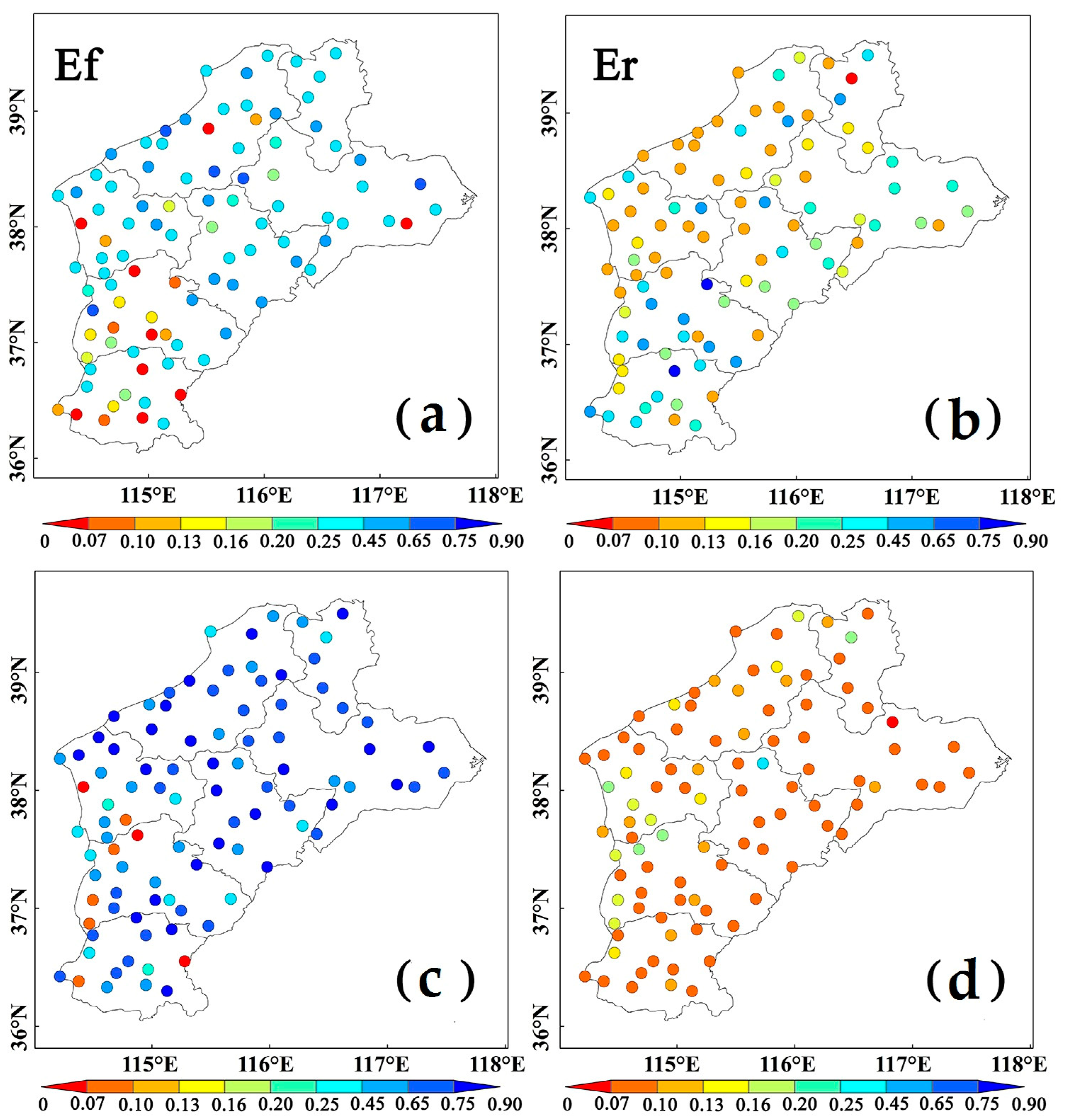
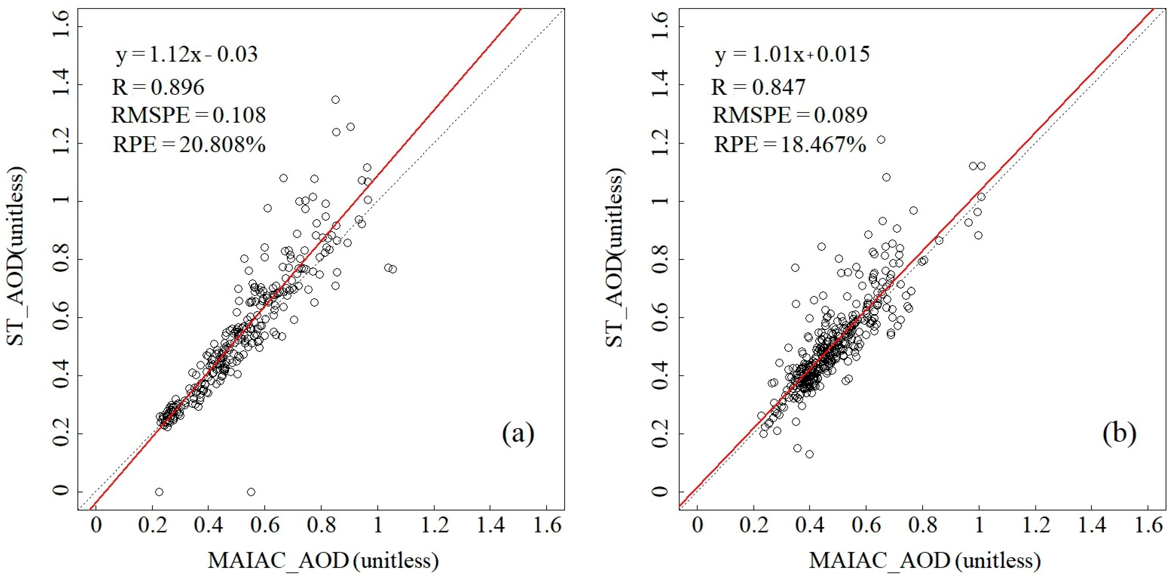
3.4. Universality Validation of ST-ERM

Analyses between the daily AOD prediction from the ST-ERM and the MAIAC AOD in 2017 were conducted to evaluate the universality and reliability of the ST-ERM.

Figure 7 shows the scatter plots of the daily ST-AOD and MAIAC AOD for all the samples. For the scatter plot results, the correlation value between daily ST-AOD and MAIAC AOD is 0.823, demonstrating that the ST-ERM can explain 67.7% of the variability for the daily AOD in 2017. Compared with the model-fitting results in 2016, the correlation R and RMSPE in 2017 decreased by 0.018 and 0.005, whereas the RPE increased by 6.53%. In addition, the slope of 0.98 in 2017 was the same as that in 2016. This finding suggests the good performance of the ST-ERM. Although the retrieved accuracy of the ST-ERM in 2017 slightly decreased, its retrieval accuracy is undoubtedly prominently improved when the ASH₁ algorithm is redefined using the ST-LME model compared with the R-ERM.

The E_f and E_r between daily MAIAC AOD and retrieved AOD by the ST-ERM in 2017 were calculated to validate the universality and reliability of the model. The E_f of the daily AOD between ST-ERM retrieval and observations (i.e., MAIAC AOD) in 2017 was greater than or equal to 0.50 at 72 of 95 stations (Figure 8). This finding indicates that the universality and reliability of the ST-ERM are good. However, there are still some stations with E_f values lower than 0.20 (Figure 8), such as 7 stations in Handan District. All these stations are located in the area with heavy air pollution. Our results also demonstrate that the E_r of daily AOD is less than 14% for all the stations, except for Shijiazhuang (17.6%), Fengfeng (17.8%), and Raoyang (30.1%). The large E_f and small E_r are generally found in central SCHP regions, such as Jinzhou, with E_f of 0.83 and E_r of 0.08%. In these areas, the ST-ERM performs well, but the stations with small E_f and large E_r are mainly located in the areas with heavy air pollution, such as Fengfeng, with E_f of −1.43 and E_r of 17.8%.

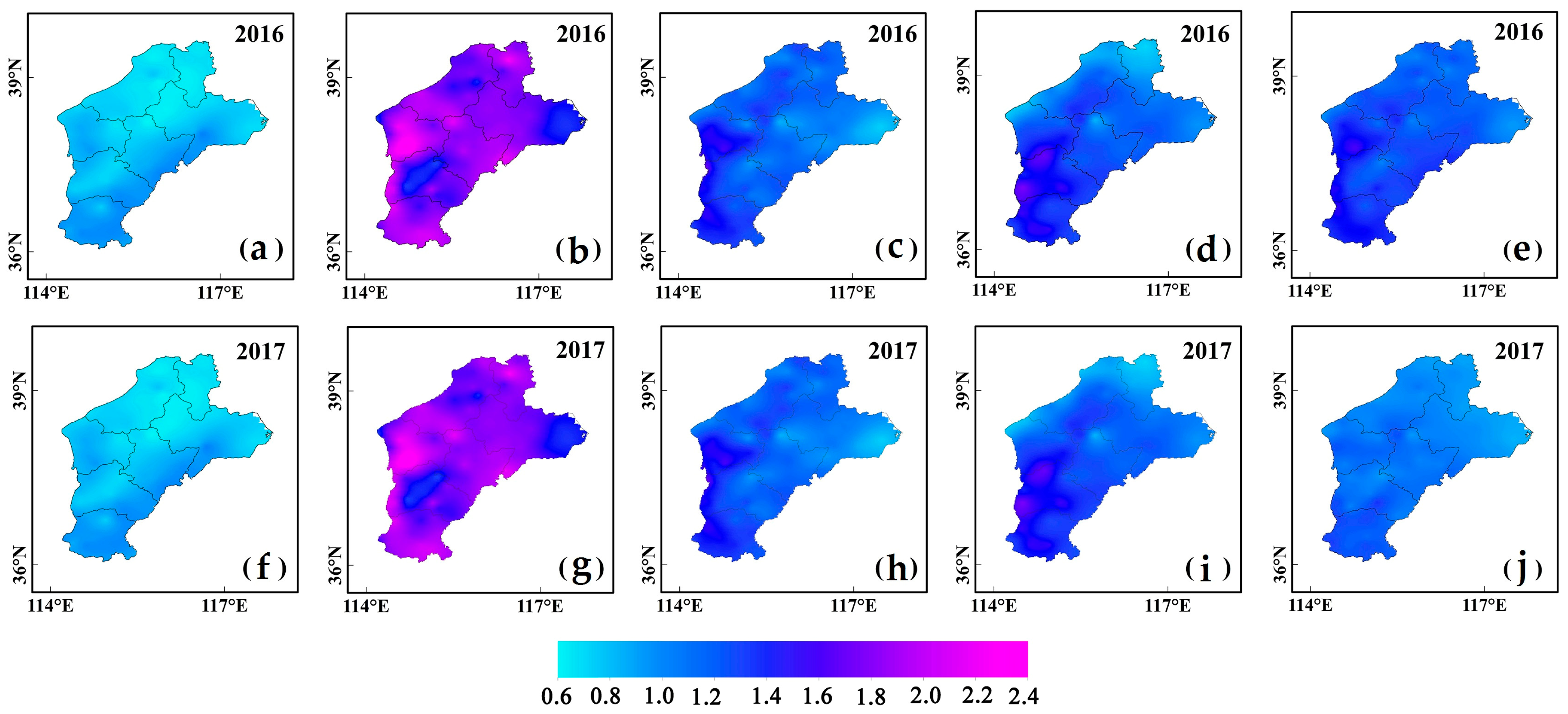
3.5. AOD Spatial Variation Characteristics

Figure 9 presents the annual mean AOD at 1 km spatial resolution using the spatiotemporal kriging interpolation method based on the retrieved AOD from the ST-ERM from 2016 (a–e) to 2017 (f–j). The results indicate that the AODs in the study domain show significant spatial variability. The regions with large AOD values are located in the southwestern areas of the SCHP, particularly in Shijiazhuang, Xingtai, and Handan Districts, with the AOD values ranging from 1.45 to 1.70 and 1.25 to 1.40 in 2016 and 2017, respectively. The northeastern areas of the SCHP are the regions with low AOD values ranging from 1.00 to 1.30 and 0 to 1.15 for 2016 and 2017, respectively. The areas with high AOD correspond well with heavily polluted industrial, densely populated, and highly urbanized regions. In comparison, low-aerosol-polluted areas are characterized by low industrial emissions, sparse population, and low urbanization levels. The topographic condition also plays an important role in AOD variation. For instance, the northeastern areas of the SCHP region, such as the Cangzhou District, are adjacent to the Bohai Sea, where the atmosphere interaction over coastal regions is conducive to the atmospheric diffusion of aerosol. By contrast, the southwestern areas of the SCHP region located in the piedmont of Taihang Mountain with poor atmospheric diffusion conditions are conducive to pollutant accumulation. Moreover, the overall AOD values over the SCHP region in 2017 were considerably lower than those in 2016. This scenario is mainly attributed to the coordinated treatment of air pollution in the Beijing–Tianjin–Hebei region in 2017, prominently reducing the air pollutant emission.

Moreover, the AODs in the SCHP region for 2016 and 2017 also present obvious seasonal variability (Figure 9). The highest AOD value, 2.4, was observed during summer. The values of AOD in the SCHP regions almost exceeded 1.5 in 2016 and 2017. This phenomenon is mainly due to two factors: first, the hygroscopic growth of the atmospheric aerosol particles caused by the high-humidity weather conditions during summer can prominently improve AOD values; second, the intense atmospheric aerosol diffusion due to beneficial weather conditions during summer, such as intense atmospheric turbulence, can greatly increase the number of atmospheric aerosol particles. By contrast, spring had the lowest AOD level, with values ranging from 0.6 to 0.8 in 2016 and 2017. The relatively low AOD level may be attributed to the low temperature and dry weather conditions, which are unfavorable to the diffusion and hygroscopic growth of aerosol particles. During the study period, similar regional AOD levels were observed in autumn and winter, with the values ranging from 0.8 to 1.4 and 0.8 to 1.8, respectively.

4. Discussion

4.1. Comparison with Other Studies with Similar Methods

In previous studies, meteorology-based AOD prediction models reveal R values for monthly AOD estimation ranging from 0.42 to 0.83 [1,2,14,24], as shown in

Table 3. Comparison of ST-ERM and similar methods on AOD prediction.

Model	Time Resolution	Study Area	Year	Model Validation				Reference
				R	RMSPE	RPE	Slope
M-Elterman	Monthly	China	2006–2009	0.42–0.83	0.047–0.102	24–54%	-	[14]
KM-Elterman	Monthly	China	2002–2010	0.71	0.208	-	0.529	[24]
R-ERM	Monthly	SCHP	2016–2017	0.69	0.20	23%	1.063–0.945	[2]
PSO-M-Elterman	Monthly	China	2007–2014	0.69–0.75	0.051–0.071	-	-	[1]
ST-ERM	Daily	SCHP	2017	0.82	0.377	63.31%	0.98	This study
ST-ERM	Monthly	SCHP	2017	0.85	0.089	18.467%	0.98	This study

. In general, the estimated accuracy of the monthly AOD prediction is higher than that of daily AOD prediction. The main reason may be that the variability of daily AOD is more difficult to estimate than that of monthly AOD because of the former’s indeterminacy caused by the random variables. Figure 10 shows the comparison of monthly mean ST-AOD and MAIAC AOD in 2016 (a) and 2017 (b). In the present study, the number of days with available MAIAC AOD data used to calculate the monthly mean AOD is more than 20 each month. Compared with the model-fitting results for the daily AOD, the R for monthly mean AOD in 2016 was 0.896, which was higher than that for daily AOD at 0.841. Moreover, the RMSPE and RPE decreased by 0.274 and 35.981%, respectively. Compared with the validation results for the daily AOD, the R for the monthly mean AOD increased by 0.24 in 2017, whereas the RMSPE and RPE decreased by 0.278 and 44.852%. These results demonstrate that the estimation accuracy of the monthly mean AOD is higher than that of the daily AOD for the ST-ERM.

In the present study, the ST-ERM outperforms the traditional deterministic R-ERM because of the accurate estimation of ASH₁, which is the key parameter for AOD prediction. The results in this study indicate that the ST-ERM achieves higher R ranging from 0.823 to 0.841 for the daily AOD prediction than the traditional R-ERM. The ST-ERM for monthly AOD prediction is also superior to the M-Elterman, KM-Elterman, and PSO-M-Elterman models in the previous study; for example, Wu et al. [14] used the M-Elterman model to retrieve the monthly AOD with the R ranging from 0.42 to 0.83 for different areas in China, and they further employed the PSO algorithm to improve the M-Elterman model with R ranging from 0.69 to 0.75. Zhang et al. [24] used the KM-Elterman model for monthly AOD prediction over China, with the R value of 0.71. In addition, the ST-ERM developed in the present study also outperforms the similar model in a previous study; for example, Li et al. [2] also redefined the ASH₁ algorithm using the multiple regression model based on meteorology to propose the R-ERM for monthly AOD prediction with the R value of 0.69.

Recently, many machine and deep-learning models, including artificial neural networks [37,39], random forest models [40,41], and extreme gradient boosted models [42], have also been used in AOD estimation. These models achieve relatively high estimation accuracy for AOD prediction. For instance, Zhang et al. [43] adopted a random forest model to estimate the AOD based on the satellite-retrieved AOD and various covariates, including meteorological conditions and land use type. Outstanding performance with an R² of 0.95 was achieved. The machine and deep-learning models are typical black box models with hidden layers and nodes [25]. These models’ performance can be improved by increasing the nodes and layers to further reveal the complex relationship between variables accurately. However, in contrast, increasing the nodes and layers may lead to overfitting in modeling. In addition, the machine and deep-learning models always require a large number of training samples, such as the available satellite-retrieved AOD and meteorological data, to develop the models by spending considerable time while yielding different results from each training period. To summarize, the ST-ERM in the present study shows a certain superiority over the machine and deep-learning models in modeling and retrieval efficiency.

4.2. Strengths and Weaknesses of the ST-ERM

In addition to its good performance, the ST-ERM can estimate the daily AOD using the daily meteorological variables from the in situ meteorological stations. In China, the network of meteorological monitoring stations provides the number of measurements required for the ST-ERM to learn the spatiotemporal relationship between AOD and variables. Compared with the conventional R-ERM, the ST-ERM prominently improves the retrieval accuracy of daily AOD with the validated R of 0.823 in 2017 because of its superior performance in handling the spatiotemporal heterogeneities of AOD variables.

The ST-ERM outperforms the conventional meteorology-based AOD model. However, the abundant spatiotemporal information from the training samples for the accurate fitting of the spatiotemporal relationship between AOD and variables greatly increases the computational workload. Furthermore, the MAIAC AOD products from MODIS only provide the data at 10:30 a.m. and 1:30 p.m. daily. This scenario further impedes the ST-ERM in retrieving the hourly AOD.

4.3. Uncertainties of ST-ERM

The ST-ERM still has a few estimation errors that are mainly attributed to the ground-level meteorological variables and the empirical parameterizations. First, the AOD represents the vertical accumulated extinction of aerosol particles, while the meteorological variables, including visibility, are measured in the surface, characterizing the variability of underlying atmosphere. Therefore, the ST-ERM requires vertical atmospheric data to learn the relationship of the variables in detail. As shown in Section 3.3, the RMSE of AOD is about 0.38, which is a relatively large value. The performance of the model can be improved by considering the vertical meteorological data, such as ERA atmospheric reanalysis data. Another uncertain is the accuracy of the empirical parameterizations, which might only be valid in certain regions, seasons, or aerosol types. To summarize, the parameters in the proposed AOD prediction model may be re-considered in other situations.

5. Conclusions

Conventional meteorology-based AOD prediction models rarely consider the spatiotemporal heterogeneity of estimation factors. As the key parameter of the AOD prediction model, the ASH₁ during the previous deterministic model studies is difficult to estimate accurately because of its complex variation. In the present study, a new ST-ERM was developed to overcome the aforementioned limitation. Compared with the conventional R-ERM, the ST-ERM can prominently improve the estimated AOD accuracy. The developed model considers the spatiotemporal heterogeneities of meteorological variables and topographic factors. Their effects on the AOD variability were also considered. The 10-fold CV and E_f approaches were employed to evaluate and compare the model’s performance.

The ST-ERM performs well using the daily MAIAC AOD as the dependent variable. A high retrieval accuracy of daily AOD was obtained with a model fitting R of 0.841, RMSPE of 0.382, and RPE of 56.789% in 2016 and a validated R of 0.823, RMSPE of 0.377, and RPE of 63.319% in 2017. The validated E_f of the daily AOD between ST-ERM predictions and observations in 2017 was greater than or equal to 0.50 at 72 of 95 stations, and the E_r was less than 14% at 92 of 95 stations. The ST-ERM outperforms the conventional meteorology-based AOD prediction models presented in previous studies, such as the R-ERM. The newly generated daily AOD has a high temporal resolution. The estimates from the ST-ERM indicate that the annual mean AOD denotes strong spatial variation showing high-in-southwest and low-in-northeast patterns in the SCHP region. In addition, the AOD estimations also show considerable seasonal variability, with the highest and lowest AOD values observed in summer and spring, respectively. The analysis results demonstrate that the accurate estimation of ASH₁ dramatically affects model performance.

Although the results are promising, some aspects of the ST-ERM can be improved in the future. For example, satellite-based AOD products with high spatiotemporal resolution would be beneficial to improving the retrieved power of the ST-ERM at a high temporal scale, such as an hourly scale. In addition, except for the natural factors, the AOD is affected by many artificial factors (e.g., land use type, road lengths, and emission information), which will be considered in future models. However, there are still some limitations for the proposed methodology in the present manuscript. Firstly, the STLME model was employed to predict the ASH₁, and it is difficult to exactly interpret the ASH₁ variation in terms of mechanism. Secondly, the proposed methodology is a statistical model based on many empirical parameterizations, which might only be valid in certain regions, seasons, or aerosol types. To summarize, the parameters in the proposed AOD prediction model may be re-considered in other regions.

References

1. Chen, B.; Ye, Y.; Tong, C.; Deng, J.; Wang, K.; Hong, Y. A novel big data mining framework for reconstructing large-scale daily MAIAC AOD data across China from 2000 to 2020. GISci Remote Sens. 2022, 59, 670–685. [Google Scholar] [CrossRef]
2. Chen, L.X.; Zhang, B.; Zhu, W.Q.; Zhou, X.J.; Luo, Y.F.; Zhou, Z.J.; He, J.H. Variation of atmospheric aerosol optical depth and its relationship with climate change in China east of 100° E over the last 50 years. Theor. Appl. Climatol. 2008, 96, 191–199. [Google Scholar] [CrossRef]
3. Chen, Y.; Shi, R.; Chao, W.; Chen, Y.; Wei, G. Estimating aerosol optical depth based on regional optimized Peterson model. J. Geogr. Inf. Sci. 2013, 15, 241. (In Chinese) [Google Scholar] [CrossRef]
4. Chen, Z.Y.; Jin, J.Q.; Zhang, R.; Zhang, T.H.; Chen, J.J.; Yang, J.; Ou, C.Q.; Guo, Y. Comparison of different missing-imputation methods for MAIAC (multiangle implementation of atmospheric correction) AOD in estimating daily PM2.5 levels. Remote Sens. 2020, 12, 3008. [Google Scholar] [CrossRef]
5. Elterman, L. Relationships between vertical attenuation and surface meteorological range. Appl. Opt. 1970, 9, 1804–1810. [Google Scholar] [CrossRef]
6. Guo, Y.; Tang, Q.; Gong, D.Y.; Zhang, Z. Estimating ground-level PM2.5 concentrations in Beijing using a satellite-based geographically and temporally weighted regression model. Remote Sens. Environ. 2017, 198, 140–149. [Google Scholar] [CrossRef]
7. Holben, B.N.; Eck, T.F.; Slutsker, I.; Tanré, D.; Buis, J.P.; Setzer, A.; Vermote, E.; Reagan, J.A.; Kaufman, Y.J.; Nakajima, T. AERONET-A federated instrument network and data archive for aerosol characterization. Remote Sens. Environ. 1998, 66, 1–16. [Google Scholar] [CrossRef]
8. Jiang, T.; Chen, B.; Nie, Z.; Ren, Z.; Xu, B.; Tang, S. Estimation of hourly full-coverage PM2.5 concentrations at 1-km resolution in China using a two-stage random forest model. Atmos. Res. 2021, 248, 105146. [Google Scholar] [CrossRef]
9. Kloog, I.; Sorek-Hamer, M.; Lyapustin, A.; Coull, B.; Wang, Y.; Just, A.C.; Schwartz, J.; Broday, D.M. Estimating daily PM2.5 and PM10 across the complex geo-climate region of Israel using MAIAC satellite-based AOD data. Atmos. Environ. 2015, 122, 409–416. [Google Scholar] [CrossRef]
10. Hoff, R.M.; Christopher, S.A. Remote sensing of particulate pollution from space: Have we reached the promised land? J. Air Waste Manag. Assoc. 2009, 59, 645–675. [Google Scholar] [CrossRef]
11. Song, Z.; Fu, D.; Zhang, X.; Han, X.; Song, J.; Zhang, J.; Wang, J.; Xia, X. MODIS AOD sampling rate and its effect on PM2.5 estimation in North China. Atmos. Environ. 2019, 209, 14–22. [Google Scholar] [CrossRef]
12. Koschmieder, H. Theorie der horizontalen Sichtweite. Beitr. Phys. Freien Atmos. 1924, 12, 171–181. [Google Scholar]
13. Levy, R.C.; Remer, L.A.; Kleidman, R.G.; Mattoo, S.; Ichoku, C.; Kahn, R.; Eck, T.F. Global evaluation of the Collection 5 MODIS dark-target aerosol products over land. Atmos. Chem. Phys. 2010, 10, 10399–10420. [Google Scholar] [CrossRef]
14. Li, F.; Zhang, L.; Wei, Q.; Yang, Y.; Han, F.; Li, W.; Zhao, C.; Wang, W. An improved method for retrieving aerosol optical depth using the ground-level meteorological data over the South-central Plain of Hebei Province, China. Atmos. Pollut. Res. 2022, 13, 101334. [Google Scholar] [CrossRef]
15. Li, L.; Franklin, M.; Girguis, M.; Lurmann, F.; Wu, J.; Pavlovic, N.; Breton, C.; Gilliland, F.; Habre, R. Spatiotemporal imputation of MAIAC AOD using deep learning with downscaling. Remote Sens. Environ. 2020, 237, 111584. [Google Scholar] [CrossRef]
16. Li, L.; Girguis, M.; Lurmann, F.; Pavlovic, N.; McClure, C.; Franklin, M.; Wu, J.; Oman, L.; Breton, C.; Gilliland, F.; et al. Ensemble-based deep Learning for estimating PM2.5 over California with multisource big data including wildfire smoke. Environ. Int. 2020, 145, 106143. [Google Scholar] [CrossRef]
17. Lin, J.; Donkelaar, A.V.; Xin, J.; Che, H.; Wang, Y. Clear-sky aerosol optical depth over East China estimated from visibility measurements and chemical transport modeling. Atmos. Environ. 2014, 95, 258–267. [Google Scholar] [CrossRef]
18. Lv, B.; Hu, Y.; Chang, H.H.; Russell, A.G.; Cai, J.; Xu, B.; Bai, Y. Daily estimation of ground-level PM2.5 concentrations at 4 km resolution over Beijing-Tianjin-Hebei by fusing MODIS AOD and ground observations. Sci. Total Environ. 2017, 580, 235–244. [Google Scholar] [CrossRef]
19. Lyapustin, A.; Martonchik, J.; Wang, Y.; Laszlo, I.; Korkin, S. Multiangle Implementation of Atmospheric Correction (MAIAC): 1. radiative transfer basis and look-up tables. J. Geophys. Res. 2011, 116, D03210. [Google Scholar] [CrossRef]
20. Lyapustin, A.; Wang, Y.; Laszlo, I.; Kahn, R.; Korkin, S.; Remer, L.; Levy, R.; Reid, J.S. Multiangle Implementation of Atmospheric Correction (MAIAC): 2. aerosol algorithm. J. Geophys. Res. 2011, 116, D03211. [Google Scholar] [CrossRef]
21. Ma, Z.; Liu, Y.; Zhao, Q.; Liu, M.; Zhou, Y.; Bi, J. Satellite-derived high resolution PM2.5 concentrations in Yangtze River Delta Region of China using improved linear mixed effects model. Atmos. Environ. 2016, 133, 156–164. [Google Scholar] [CrossRef]
22. McClatchey, R.A.; Fenn, R.W.; Selby, J.E.A. Optical Properties of the Atmosphere; Air Force Cambridge Research Lab: Bedford, UK, 1972. [Google Scholar]
23. Meng, X.; Liu, C.; Zhang, L.; Wang, W.; Liu, Y. Estimating PM2.5 concentrations in Northeastern China with full spatiotemporal coverage, 2005–2016. Remote Sens. Environ. 2021, 253, 112203. [Google Scholar] [CrossRef] [PubMed]
24. Peterson, J.T.; Fee, C.J. Visibility-atmospheric turbidity dependence at Raleigh, North Carolina. Atmos. Environ. 1981, 15, 2561–2563. [Google Scholar] [CrossRef]
25. Qin, W.; Wang, L.; Lin, A.; Zhang, Z.; Bilal, M. Improving the estimation of daily aerosol optical depth and aerosol radiative effect using an optimized artificial neural network. Remote Sens. 2018, 10, 1022. [Google Scholar] [CrossRef]
26. Qiu, J.H.; Lin, Y. A parametric model for the optical depth of atmospheric aerosols in China. Acta Meteorol. Sin. 2001, 59, 368–372. (In Chinese) [Google Scholar]
27. Retalis, A.; Hadjimitsis, D.G.; Michaelides, S.; Tymvios, F.; Chrysoulakis, N.; Clayton, C.; Themistocleous, K. Comparison of aerosol optical thickness with in situ visibility data over Cyprus. Nat. Hazard. Earth Sys. 2010, 10, 421–428. [Google Scholar] [CrossRef]
28. She, L.; Zhang, H.K.; Li, Z.; de Leeuw, G.; Huang, B. Himawari-8 Aerosol Optical Depth (AOD) retrieval using a deep neural network trained using AERONET observations. Remote Sens. 2020, 12, 4125. [Google Scholar] [CrossRef]
29. Sun, X.; Yin, Y.; Sun, Y.; Sun, Y.; Liu, W.; Han, Y. Seasonal and vertical variations in aerosol distribution over Shijiazhuang, China. Atmos. Environ. 2013, 81, 245–252. [Google Scholar] [CrossRef]
30. Tang, W.; Yang, K.; Qin, J.; Niu, X.; Lin, C.; Jing, X. A revisit to decadal change of aerosol optical depth and its impact on global radiation over China. Atmos. Environ. 2017, 150, 106–115. [Google Scholar] [CrossRef]
31. Wang, K.; Dickinson, R.E.; Liang, S. Clear sky visibility has decreased over land globally from 1973 to 2007. Science 2009, 323, 1468–1470. [Google Scholar] [CrossRef]
32. Wang, W.; He, J.; Miao, Z.; Du, L. Space–time linear mixed-effects (STLME) model for mapping hourly fine particulate loadings in the Beijing–Tianjin–Hebei region, China. J. Clean. Prod. 2021, 292, 125993. [Google Scholar] [CrossRef]
33. Wu, J.; Luo, J.; Zhang, L.; Xia, L.; Zhao, D.; Tang, J. Improvement of aerosol optical depth retrieval using visibility data in China during the past 50 years. J. Geophys. Res. Atmos. 2014, 119, 13370–13387. [Google Scholar] [CrossRef]
34. Wu, J.; Zhang, S.; Yang, Q.; Zhao, D.; Fan, W.; Zhao, J.; Shen, C. Using particle swarm optimization to improve visibility-aerosol optical depth retrieval method. npj Clim. Atmos. Sci. 2021, 4, 49. [Google Scholar]
35. Xiao, Q.; Geng, G.; Cheng, J.; Liang, F.; Li, R.; Meng, X.; Xue, T.; Huang, X.; Kan, H.; Zhang, Q. Evaluation of gap-filling approaches in satellite-based daily PM2.5 prediction models. Atmos. Environ. 2021, 244, 117921. [Google Scholar] [CrossRef]
36. Zhang, R.; Di, B.; Luo, Y.; Deng, X.; Grieneisen, M.L.; Wang, Z.; Yao, G.; Zhan, Y. A nonparametric approach to filling gaps in satellite-retrieved aerosol optical depth for estimating ambient PM2.5 levels. Environ. Pollut. 2018, 243, 998–1007. [Google Scholar] [CrossRef]
37. Zhang, S.; Wu, J.; Fan, W.; Yang, Q.; Zhao, D. Review of aerosol optical depth retrieval using visibility data. Earth Sci. Rev. 2020, 200, 102986. [Google Scholar] [CrossRef]
38. Zhang, Z.; Wu, W.; Wei, J.; Song, Y.; Yan, X.; Zhu, L.; Wang, Q. Aerosol optical depth retrieval from visibility in China during 1973–2014. Atmos. Environ. 2017, 171, 38–48. [Google Scholar] [CrossRef]
39. Zhang, Z.Y.; Wu, W.L.; Fan, M.; Wei, J.; Tan, Y.; Wang, Q. Evaluation of MAIAC aerosol retrievals over China. Atmos. Environ. 2019, 202, 8–16. [Google Scholar] [CrossRef]
40. Zhao, B.; Wang, S.; Ding, D.; Wu, W.; Chang, X.; Wang, J.; Xing, J.; Jang, C.; Fu, J.S.; Zhu, Y.; et al. Nonlinear relationships between air pollutant emissions and PM2.5-related health impacts in the Beijing-Tianjin-Hebei region. Sci. Total Environ. 2019, 661, 375–385. [Google Scholar] [CrossRef]
41. Zhao, C.; Liu, Z.; Wang, Q.; Ban, J.; Chen, N.X.; Li, T. High-resolution daily AOD estimated to full coverage using the random forest model approach in the Beijing-Tianjin-Hebei region. Atmos. Environ. 2019, 203, 70–78. [Google Scholar] [CrossRef]
42. Zhong, J.; Zhang, X.; Gui, K.; Wang, Y.; Che, H.; Shen, X.; Zhang, L.; Zhang, Y.; Sun, J.; Zhang, W. Robust prediction of hourly PM2.5 from meteorological data using LightGBM. Natl. Sci. Rev. 2021, 8, 115–126. [Google Scholar] [CrossRef] [PubMed]
43. Zhou, M.; Wang, J.; Chen, X.; Xu, X.; Colarco, P.R.; Miller, S.D.; Reid, J.S.; Kondragunta, S.; Giles, D.M.; Holben, B. Nighttime smoke aerosol optical depth over U.S. rural areas: First retrieval from VIIRS moonlight observations. Remote Sens. Environ. 2021, 267, 112717. [Google Scholar] [CrossRef]
Figure 1. Geospatial distribution of the meteorological stations over the study area. Each black dot in the figure denotes a monitoring site.
Sustainability 15 02609 g001
Figure 2. Correlations between MAIAC AOD and AERONET AOD in 2016 (a) and 2017 (b).
Sustainability 15 02609 g002
Figure 3. Frequency distribution histogram of parameters of modeled data in SCHP in 2016.
Sustainability 15 02609 g003
Figure 4. Comparison of observed and retrieved daily ASH1 for ST-LME model fitting (a) and 10-fold cross-validation (b) in 2016. The black dotted line is the 1:1 line, and the red solid line is the model regression line.
Sustainability 15 02609 g004
Figure 5. Comparison between daily MAIAC AOD and R-AOD (a)/ST-AOD (b) in 2016. The black dotted line is the 1:1 line, and the red solid line is the model regression line.
Sustainability 15 02609 g005
Figure 6. Comparisons of Ef and Er between daily MAIAC AOD and retrieved AODs by R-ERM (a,b), and ST-ERM (c,d) at the 95 meteorological stations in 2016.
Sustainability 15 02609 g006
Figure 7. Assessment of ST-ERM performance based on observed and retrieved daily AOD for the model’s applicability. The red solid line represents the regression line, and the dashed line represents the 1:1 line.
Sustainability 15 02609 g007
Figure 8. The spatial distribution of Ef and Er by ST-ERM for SCHP region in 2017.
Sustainability 15 02609 g008
Figure 9. Seasonal (spring (a,f), summer (b,g), autumn (c,h), and winter (d,i)) and annual (e,j) mean AOD concentrations in 2016 and 2017 over the SCHP region.
Sustainability 15 02609 g009
Figure 10. Comparisons between monthly MAIAC AOD and ST-AOD for 2016 (a) and 2017 (b). The black dotted line is the 1:1 line, and the red solid line is the model regression line.
Sustainability 15 02609 g010