Numerical Investigation of a Local Precise Reinforcement Method for Dynamic Stability of Rock Slope under Earthquakes Using Continuum–Discontinuum Element Method

Abstract

The slope reinforcement scheme has an important influence on the prevention and control of landslides. A reasonable reinforcement scheme can improve the reliability, economy and efficiency of landslide resistance. It is urgent to establish a local precise reinforcement method for landslides on the basis of clear process and the instability modes of landslides. Taking a high-steep anti-dip rock slope as an example, six numerical models are established by using the continuum–discontinuum element method (CDEM) to carry out seismic damage and dynamic analysis of slopes. By comparing the seismic response and damage characteristics of being unstrengthened, local precise reinforcement and overall reinforcement models, the applicability of the proposed local precise reinforcement method for the slopes is discussed. The results show that the determination of the dynamic amplifying effect and seismic damage characteristics of slopes is the primary prerequisite of the local precise reinforcement method. The dynamic amplification effect of the slope toe, crest and shallow slope surface are much larger, that is, they are the potential reinforcement areas. The local precision reinforcement times should be controlled within a certain number of times, and the slope after the first three times of the local reinforcement effect is the best. However, more than three times after the reinforcement effect it becomes worse. Moreover, the dynamic amplification effect, the equivalent crack ratio and the mechanical energy of the slope after three times of local precision reinforcement are similar to the overall reinforcement effect, which indicates that local precision reinforcement has good feasibility. This work can provide references for landslide disasters prevention and control.

1. Introduction

The topography, geology and climate in China are extremely complex, with seven major water systems, five major earthquake zones and twenty-three seismic zones [1]. The coupling effect of earthquake, meteorology, water and other disaster-causing factors intensifies the frequency and scale of landslide disasters, which has a significant impact on the construction and operation safety of major water conservancy and traffic projects [2]. Landslide disaster is one of the main natural disasters in the world, and has become a geological disaster which seriously threatens people’s lives and properties [3]. Due to the effects of earthquake, groundwater, geological conditions and other factors, the triggers and disaster process of landslide disasters has become extremely complicated [4,5]. Slope reinforcement is helpful to ensure the stability of geotechnical engineering slopes, which is an important measure to ensure the stability of slopes, and can also essentially eliminate the adverse factors of slope stability [6]. The choice of the slope reinforcement scheme has an important influence on the prevention and control of landslide disasters [7]. A reasonable reinforcement scheme can improve the economy and safety of landslide disaster prevention and control [8,9]. In particular, the earthquake damage evolution process of complex slopes under earthquakes has the characteristics of accumulation and being gradual, which makes the prevention and control of earthquake damage of the slope more difficult. Therefore, it is of great engineering significance to investigate slope damage reinforcement under earthquakes.

Many geological elements, such as rock lithology, structural plane, weathering, unloading, ground stress, groundwater, landform and other geological elements, are the main influencing factors of slope stability and safety [10,11]. It is necessary to use engineering geological investigation technology and geotechnical testing technology to find out the engineering geology and hydrogeological conditions of slopes, and to provide geological data and a basis for engineering designs by analyzing and predicting the engineering geological problems of slopes [12]. At present, a lot of research progress has been made on the prevention and control measures of slopes. Ma et al. reinforced the rock slope after the excavation of large-scale water conservancy and hydropower, and studied the effects of slope reinforcement with microseismic technology, and discussed the influence of reinforcement measures on slope stability [13]. Liu et al. adopted water-based polyurethane soil stabilizer to strengthen the sandy soil slope to achieve the purpose of erosion prevention, and discussed the reinforcement effect, and proved the feasibility of polyurethane treatment in practice [14]. Fan et al. used the large-scale shaking table test to study the dynamic response of slopes reinforced by double-row anti-slide piles and prestressed anchor cables, and discussed the influence of two anti-slide pile reinforcement measures on the dynamic response characteristics of slopes [15]. Chen et al., based on the strength reduction method, adopted piles, retaining walls, porous steel pipe grouting and other methods to consolidate an open-pit slope, and discussed the reinforcement effect of the slope and the feasibility of the reinforcement methods [16]. Wang et al. used the finite element method to study the action mechanism of pile foundations in slopes, and studied the influence of the position and length of a pile foundation on the stability of an embankment [17]. Li et al. investigated the disaster mechanism and trigger factors of an abandoned mine slope based on laboratory experiments and field investigations, and proposed slope reinforcement and ecological restoration measures by adding green planting [18]. Zhang et al. discussed the theory and method of the elastic design of flexible supporting expansive soil slopes based on long-term field monitoring tests, in order to improve the resistance, recovery and adaptability of flexible supporting structures to the failure of expansive soil slopes [19]. Zhang et al. adopted the numerical simulation method to discuss the pile–soil interaction mechanism and optimal use of the slope reinforced by an anti-slide pile, and analyzed the force displacement principle of the slope and anti-slide pile [20]. Liu et al. used physical model experiments to study the deformation characteristics and evolution mechanisms of reservoir landslides and pile systems under the action of reservoir water [21]. At present, there are many slope reinforcement measures available, but they can be summarized into the following categories: load reduction measures, drainage and water interception measures, anchorage measures, concrete shear structure measures, retaining measures and slope pressure measures [22,23,24]. A reasonable reinforcement scheme can not only improve the reliability of landslide disaster prevention, but also save costs to a large extent and improve the efficiency of construction and prevention [25,26].

The prevention and control of landslide disasters is mainly based on the investigation of existing landslide disasters or the monitoring of landslide deformation to determine whether to carry out reinforcement treatment [26,27]. The deformation characteristics, evolution trends and instability modes of landslides are not clear before slope reinforcement, which will inevitably have many adverse effects on the reinforcement effect of slopes. On the basis of field investigation and on-site monitoring, when a slope deformation or sliding trend is found, slope reinforcement is selected. At this time, the slope reinforcement plan, time point and reinforcement area are determined. In the whole process of landslide evolution, it is difficult to accurately reinforce the dangerous area of the slope, and it is difficult to effectively curb the slope deformation and landslide disaster prevention. The prevention and control of landslide disasters is mainly based on the investigation of existing landslide disasters or the monitoring of landslide deformation to determine whether to carry out reinforcement treatment [28]. However, most of the previous slope reinforcement measures and design methods are guided by passive remediation measures after problems occur, while there are few studies on active remediation measures [29]. Moreover, in the past, slope reinforcement methods were mainly large-scale reinforcements, but few precise reinforcement measures have been taken. The previous protection methods have the characteristics of being extensive and excessive, or there is a potential deformation and failure risk of slopes for timely detection and reinforcement measures. Slope prevention and control technology is not accurate, it is difficult to carry out precise targeted reinforcements of slopes, it greatly increases the cost of engineering construction and operation and maintenance and it causes huge losses to the national economy [30,31]. Therefore, it is necessary to propose a local precise, targeted protection method of slopes, to adopt appropriate monitoring methods to identify and predict the stability of engineering slopes and to establish the whole process of slope protection measures of “precise reinforcement time, precise reinforcement target and fine deformation control”.

In order to solve the existing problems in the existing technology, the purpose of this work is to provide a local precise targeted protection method for slope stability identification and prediction and its precise targeted protection. Taking an anti-dip rock slope in eastern Tibet, China as an example, this work explores the beneficial effects and feasibility of the proposed local precision reinforcement method through numerical simulation. This method illustrates the principle of the time-sharing and zonal precise targeted reinforcement method for the slope. The continuous and discontinuous coupled numerical simulation method is used to analyze the ground motion of the slope, to identify and predict the danger area of the slope’s stability and to determine the best time, target position and required reinforcement load of slope reinforcement. A reasonable local precise targeted reinforcement scheme for the slope was developed, and the effects of different reinforcement measures were compared and analyzed by the numerical simulation method to verify the economy and reliability of the proposed time-sharing and zonal precise targeted reinforcement scheme. This method improves the cognitive level of engineering technicians and researchers on slope protection. This method greatly improves the accuracy, reliability and economy of slope disaster protection, and has wide application prospects in the field of geotechnical engineering geological disaster prevention.

2. Methodology

2.1. Case Study

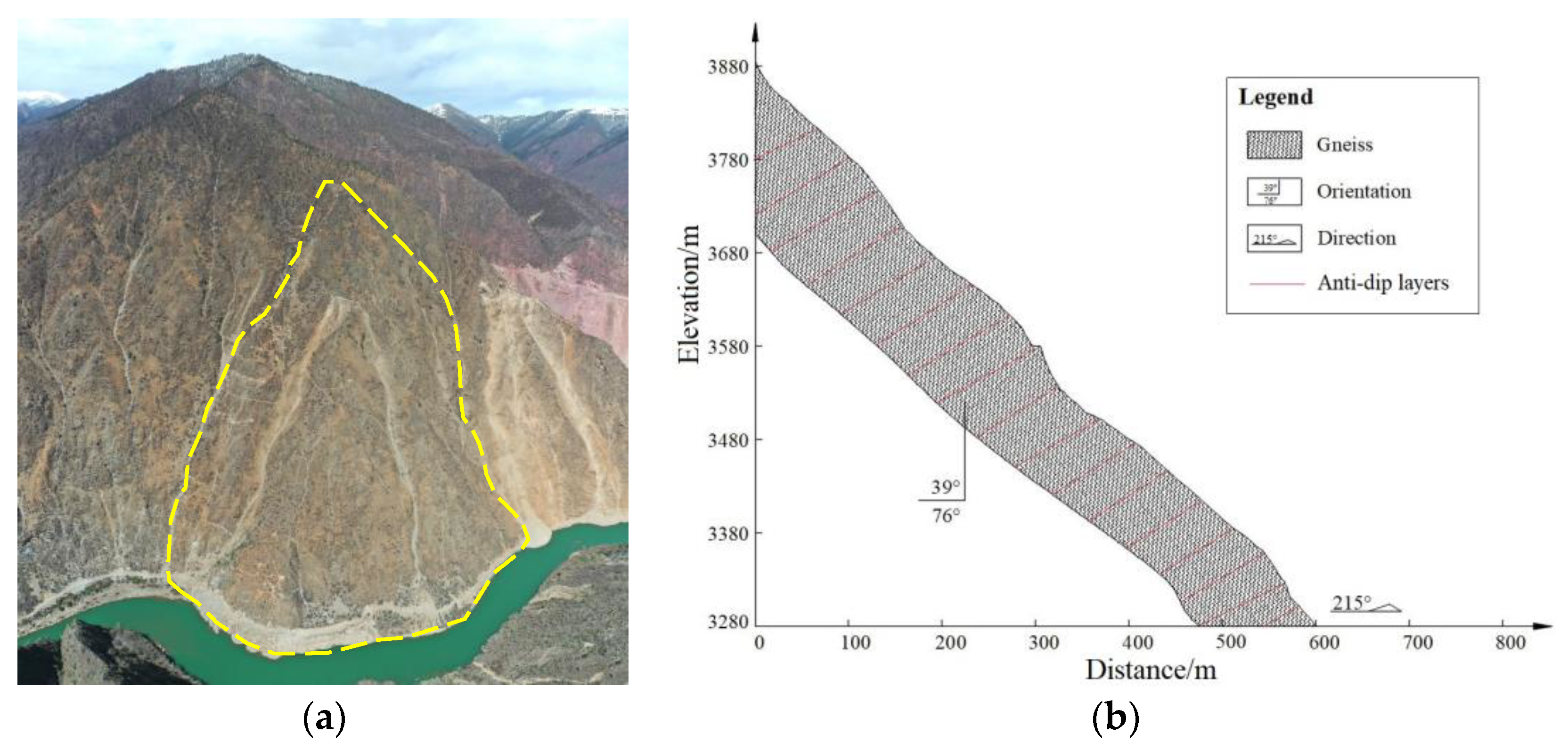
The study area is located in a region of high seismic intensity in western China, which is located in the eastern Tibet Province. The geographical location of the study area is shown in Figure 1. The geomorphology and engineering geological profile of the anti-dip slope is shown in Figure 2. There are several faults in the study area, and ground motion occurs frequently. The stability of slope in the study area is greatly affected by earthquakes. The slope belongs to high and steep rock slope with large height difference. The shape of the slope shows “tongue” type as a whole. The elevation of the slope toe is about 3280 m, and the elevation of the slope crest is about 3880 m, and the slope height is about 600 m. The slope is about 994 m long and 530 m wide. The slope direction is about 185°, the average gradient is 60–75° and the bedrock occurrence is 39° < 76°. The slope is a typical anti-dip rock mass slope, including several anti-dip planes and fissures. The bedrock of the slope is the granitic gneiss of the Paleo-Mesoproterozoic Jitang Group (Pt1-2Gn) with relatively developed joints. The overlying accumulation body consists of gray–yellow landslide rubble soil and fine breccia soil, and the content of gravel is about 50–70%, and the sorting and roundness are poor. According to the sample study of the typical weathered gneiss, the weathered gneiss on the slope surface is yellowish brown and retains the original rock structure basically. Quartz and biotite and other minerals are found, which can be easily crumbled by hand. Physical and mechanical parameters of gneiss were obtained through indoor basic geotechnical tests, as shown in

Table 1. Parameters of block elements in the numerical calculation.

Name	ρ [kg/m3]	E [GPa]	ν [-]	c [kPa]	T [kPa]	Φ [°]
Rock	2600	28.7	0.24	16.9	8.05	63.2

.

2.2. Basic Principles of Numerical Model Calculation

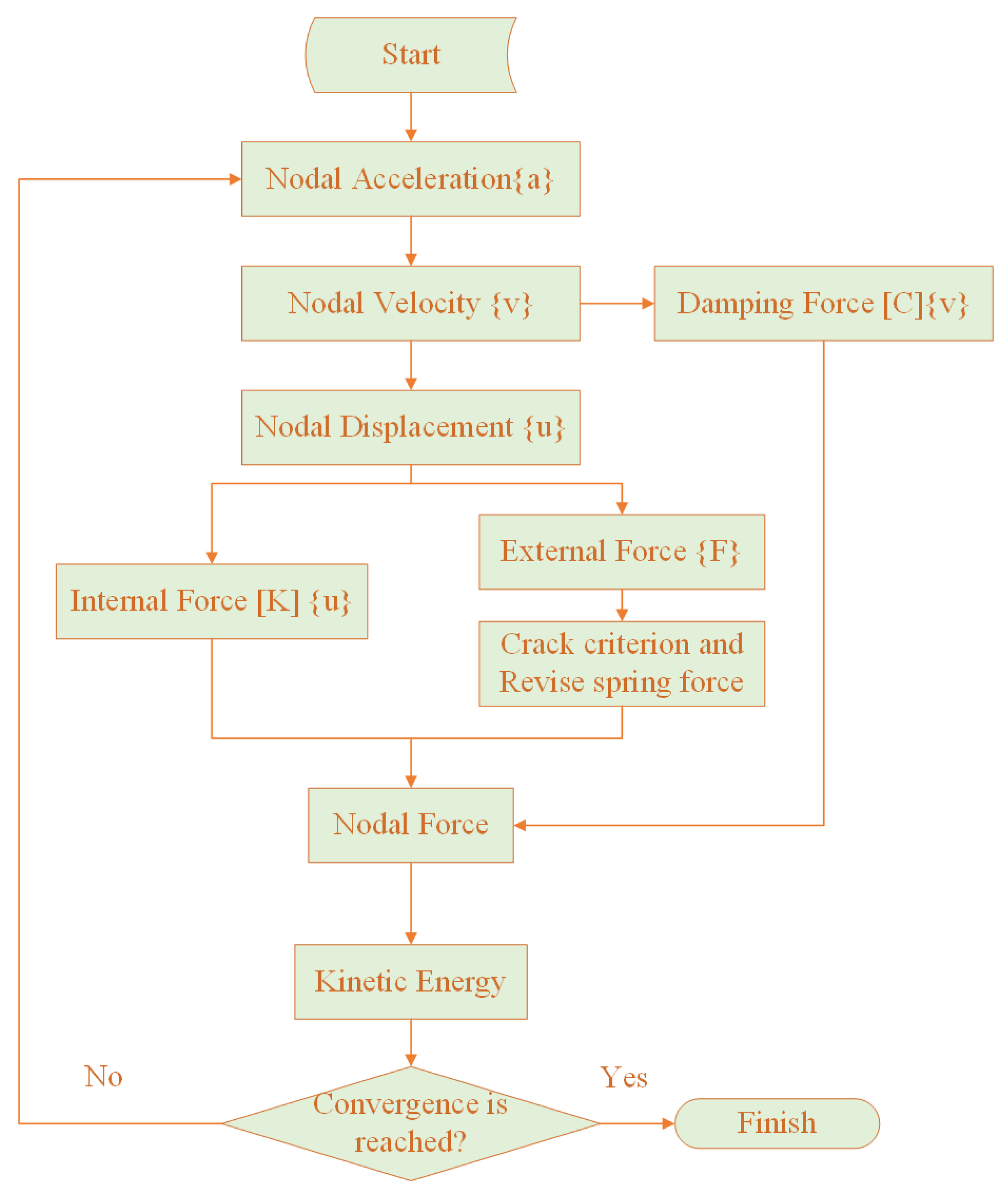
The calculation domain is discretized into continuous elements, discontinuous elements and partially continuous elements in numerical calculation, which, respectively, correspond to the finite element method (FEM) domain, discrete element method (DEM) domain and continuum–discontinuum element method (CDEM) domain, as shown in Figure 3. FEM is applicable to completely continuous problems, and DEM is applicable to completely discontinuous problems. CDEM carries out finite element calculation inside the block and discrete element calculation at the boundary, which is mainly used to simulate the progressive failure process of rock–soil mass from continuous medium to discontinuous medium [32]. The contact relationship of the numerical model is shown in Figure 4. The block is composed of one or more finite element elements, which are used to characterize the continuous properties of materials such as elasticity, plasticity and damage. The common boundary between the two blocks is the interface, which is used to characterize the discontinuous properties of materials such as fracture, slip and collision. The block is composed of finite elements to characterize the continuous characteristics of rock. The characteristic of CDEM is that it can simulate the initiation, propagation and connection of explicit cracks in materials while simulating the elastic–plastic deformation of materials. Interfaces in CDEM include two concepts: real interface and virtual interface. The real interface is used to represent the interface, fault, joint and other real discontinuous surfaces of materials, and its strength parameters are consistent with those of the real interface. The virtual interface mainly has two functions [33]: (1) connect two blocks for transferring mechanical information; (2) provide a potential channel for the propagation of explicit cracks (that is, cracks can propagate along any virtual interface). In the modeling process, the MC model is adopted for the element, and the brittle fracture model based on MC criteria is adopted for the contact. Considering the difference between rocks and between layers, the contact parameters between bedding are smaller than those within rocks. The schematic diagram of CDEM calculation process is shown in Figure 5.

CDEM uses explicit Euler forward difference method based on incremental mode to solve dynamic problems, which mainly includes two parts: joint force calculation and node movement calculation. The tensile shear composite interface constitutive model considering fracture energy is used to calculate the fracture of rock virtual interface. F_n and F_s are the normal and tangential connection force, respectively.

The normal and tangential detecting contact forces of adjacent time steps on the virtual interface are as follows [32,34]:

$$F_n(t_1)=F_n(t_0)-k_n{A}_c\mathsf{\Delta }{\mu }_n,\hspace{1em}{F}_s(t_1)=F_s(t_0)-k_s{A}_c\mathsf{\Delta }{\mu }_s.$$

(1)

where k_n and k_s are the normal and tangential connection stiffness, respectively; $A$_c is the area of the virtual interface; ∆μ_n and ∆μ_s are the relative displacement increment in normal and tangential directions, respectively. The tensile failure criterion considering the tensile fracture energy is expressed as follows:

$$if-F_n(t_1)\ge {\sigma }_t(t_0)A_c\begin{array}{cc},& \begin{array}{cc}then& \end{array}Fn(t_1)\end{array}=-{\sigma }_t(t_0)A_c{\begin{array}{cc},& {\sigma }_1(t_1)=-({\sigma }_{t_0})\end{array}}^2\mathsf{\Delta }{u}_n/(2G_{f}t)+c_0.$$

(2)

where σ_t0, σ_t(t₀) and σ_t(t₁) are the tensile strengths on the virtual interface at the different moments. G_ft is the tensile fracture energy.

The shear failure criterion considering shear fracture energy is:

$$F_s(t_1)\ge F_n(t_1)\tan \phi +c(t_0)A_c\begin{array}{cc},& F_s(t_1)=F_n(t_1)\tan \phi +c(t_0)A_c\end{array}\begin{array}{cc},& c(t_1)=-c_0{}^2\mathsf{\Delta }{u}_s/(2G_{f}s)\end{array}+c_0.$$

(3)

where c₀, c(t₀) and c(t₁) are the cohesion on the virtual interface at the different moments, and the φ is the corresponding internal friction angle.

CDEM is a dynamic explicit solution algorithm based on breakable elements under the Lagrangian system. The core control equation is:

$$M\ddot{u}+C\dot{u}+Ku+K_c{u}_c+C_c{\dot{u}}_c=F.$$

(4)

CDEM uses the explicit Euler forward difference method based on incremental method to solve the problem. In this work, a continuous and discontinuous numerical model (anti-dip rock slope) is established, which consists of seventeen anti-dip contact layers. The gradient of the slope is about 60° and the dip angle of the anti-tip contact layers is about 165°. The slope numerical model adopts the continuous–discontinuous element method of integrated finite element method and discrete element method. The solid element adopts the ideal elastoplastic model based on Mohr–Coulomb criterion. The interface unit of rock mass is composed of virtual spring, and its failure obeys the energy fracture criterion. Explicit forward difference method is used to solve this method. In the static equilibrium stage, the maximum unbalance force (1 × 10⁻⁵) is taken as the convergence standard. In the phase of dynamic calculation, time is taken as the standard to end the calculation, and the calculation ends when the preset calculation time (ground motion lasting 20 s) is reached. The numerical simulation process is as follows: Firstly, the initial model is simulated. For the numerical model, five working conditions (0.1, 0.2, 0.3, 0.4 and 0.5 g) were selected to carry out dynamic analysis, and these seismic waves were loaded at the bottom of the model. By observing the seismic damage of the slope, the slope toe is destroyed first. The first model is the slope model without reinforcement. In the second model, the local area at the foot of the slope is reinforced, and the model is simplified, that is, in the parameters of the block and the contact surface within the reinforcement range, the cohesion is increased by 10 times. The third model is to reinforce the local area of the slope surface by grouting (within 10 m depth of the slope surface), and the reinforcement method still has a 10 times greater cohesion. The fourth model is to reinforce the local area of the slope top. The fifth model is to strengthen the local area of the slope top and foot, and the reinforcement method is to increase the cohesion by 10 times. The sixth model is the overall strengthening condition. In order to compare and analyze the effect of local reinforcement, unreinforcement and overall reinforcement conditions, the calculation conditions are divided into the following 6 cases, as shown in

Table 2. Calculation conditions in numerical simulation.

No.	Slope Strengthening Conditions
Case 1	Slope without reinforcement
Case 2	Slope after the first reinforcement (grouting reinforcement at the slope toe)
Case 3	Slope after the second reinforcement (grouting reinforcement at the shallow slope surface)
Case 4	Slope after the third reinforcement (grouting reinforcement at the slope crest)
Case 5	Slope after the fourth reinforcement (grouting reinforcement at the shallow slope surface and slope toe)
Case 6	Slope after the integral reinforcement

.

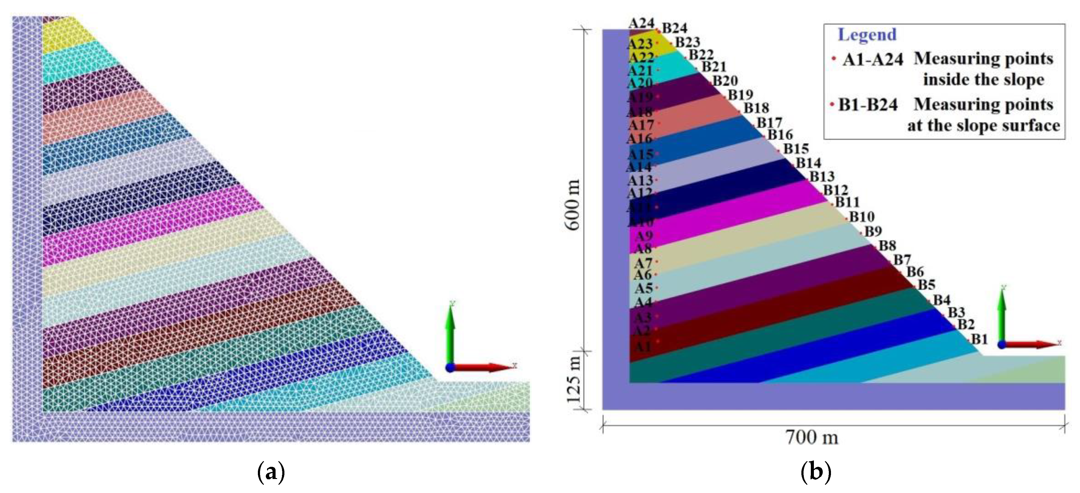
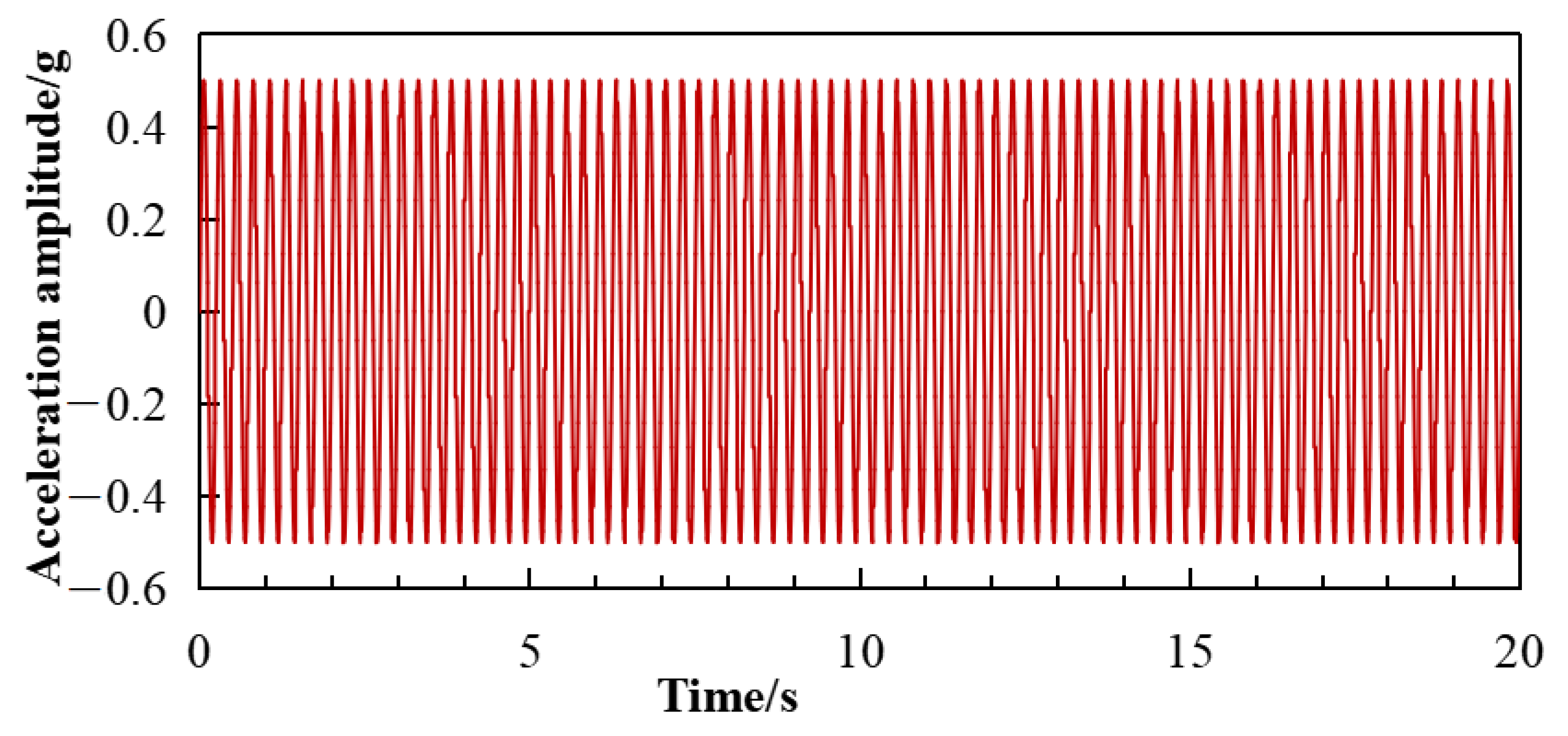
The numerical model of the slope is shown in Figure 6. The layout scheme of monitoring points in the model is shown in Figure 6b. Sinusoidal waves are loaded at the bottom of the model slopes to simulate ground motion. The slopes are 725 m high and 700 m long. In numerical simulation, viscous boundary was used at the bottom of the models and free field was used at both sides of the models to eliminate the adverse influence of boundary conditions. The direction displacement at the bottom of the models is fixed. The acceleration time–history curve of loaded harmonic waves are shown in Figure 7.

It is worth noting that in CDEM calculation, seismic load in the form of stress time history can only be loaded on the viscous boundary, hence, it is necessary to convert the acceleration time–history curve into the velocity–time–history curve, then into the stress–time–history, and finally apply it on the viscous boundary. When the seismic wave is loaded at the bottom of the model, only the stress boundary condition of vibration can be applied as the ground motion input due to the limitation of the calculation method. In this work, the error in the conversion process from acceleration–time–history curve to velocity–time–history curve and then to stress–time–history curve can be avoided effectively by using simple harmonic input. The transformation of velocity–time–history into stress–time–history is as follows:

$${\sigma }_n=2(p\cdot C_p)v_n\begin{array}{cc},& \end{array}{\sigma }_s=2(p\cdot C_s)v_s.$$

(5)

where, C_s and C_p are the velocities of S-wave and P-wave; v_s and v_n are tangential and normal velocities. In CDEM, parameter selection is very important for the reliability and accuracy of calculation results. Among them, the selection of numerical spring parameter and volume parameter is very important. Numerical spring parameter represents the discontinuity feature of the model, while volume parameter represents the continuity feature of the model. The combination of the two together plays a continuous to discontinuous simulation process in CDEM calculation, as shown

Table 3. Parameters of the contact elements in the numerical calculation.

Working Condition	Name	kn [GPa/m]	ks [GPa/m]	c [kPa]	T [kPa]	Φ [°]	GfI [Pa·m]	GfII [Pa·m]
Before grouting reinforcement	Block interface	300	300	16.9	8.05	63.2	10	50
	Layer interface	300	300	0.1	0.1	20	0	0
After grouting reinforcement	Rock interface	300	300	16.9	8.05	63.2	10	50
	Layer interface	300	300	16.9	8.05	63.2	10	50

.

3. Results

3.1. Evaluation of Slope Stability after Partial Reinforcement

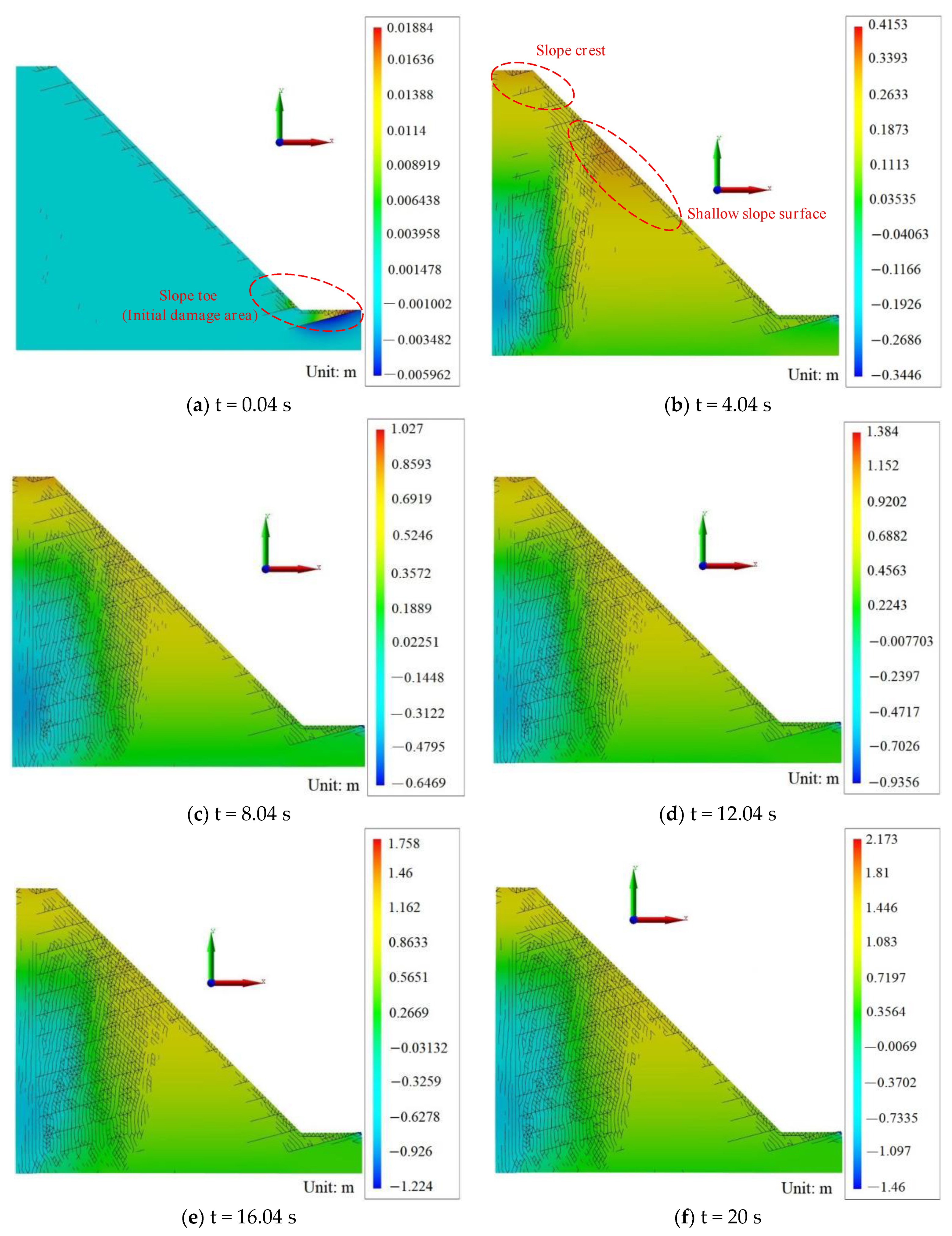
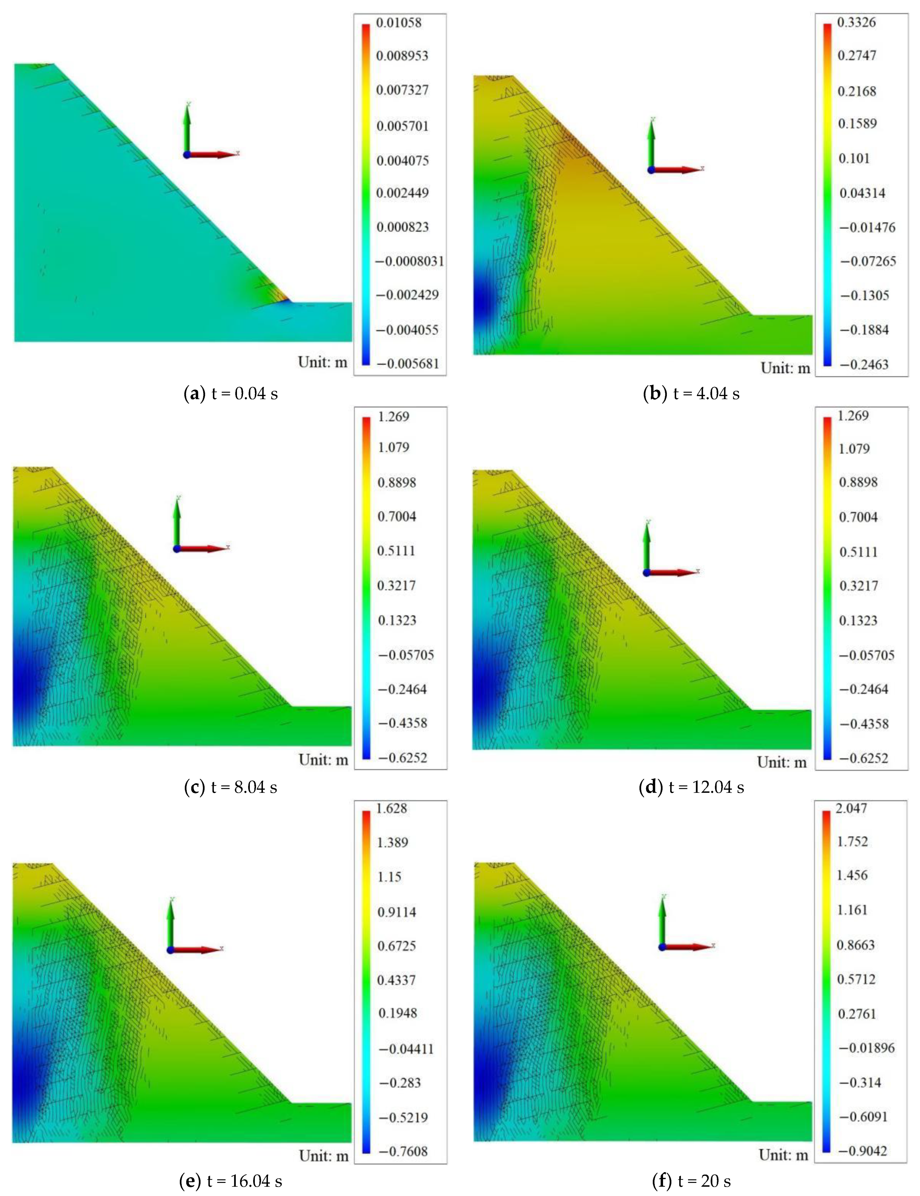
The displacement distribution of the slope under the loading of 0.5 g horizontal seismic wave is shown in Figure 8. Figure 8 shows that when t = 0.04 s, the initial damage first appears at the slope toe. With the continuous ground motion, the maximum displacement of the slope gradually appears in the shallow slope surface and the slope crest area. The maximum displacement of the slope is 2.173 m. Therefore, the slope toe, surface and crest have become the key areas of concern and potential deformation danger area. That is, these areas are also the key areas to be strengthened. Firstly, Case 2 was locally strengthened at the slope toe. When 0.5 g horizontal ground motion was applied, the displacement distribution of the slope is shown in Figure 9. Figure 9 shows that during the process of earthquake, the slope deformation and damage first appear on the slope surface, and gradually intensify with the increase in ground motion time. The maximum displacement of the slope after the first grouting reinforcement at the slope foot is about 2.016 m. The displacement of the model after the first reinforcement is significantly reduced compared with that before the first reinforcement.

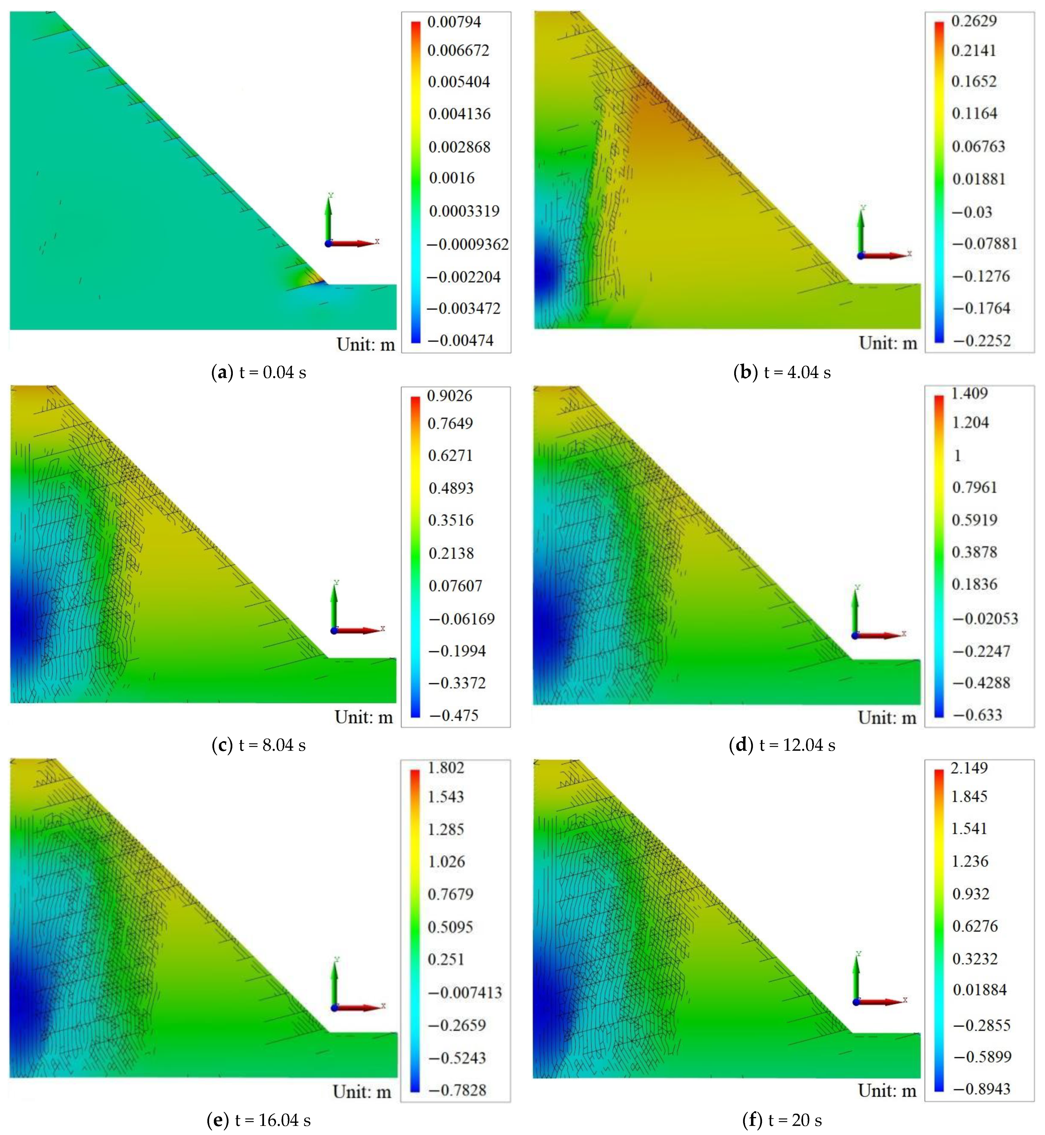
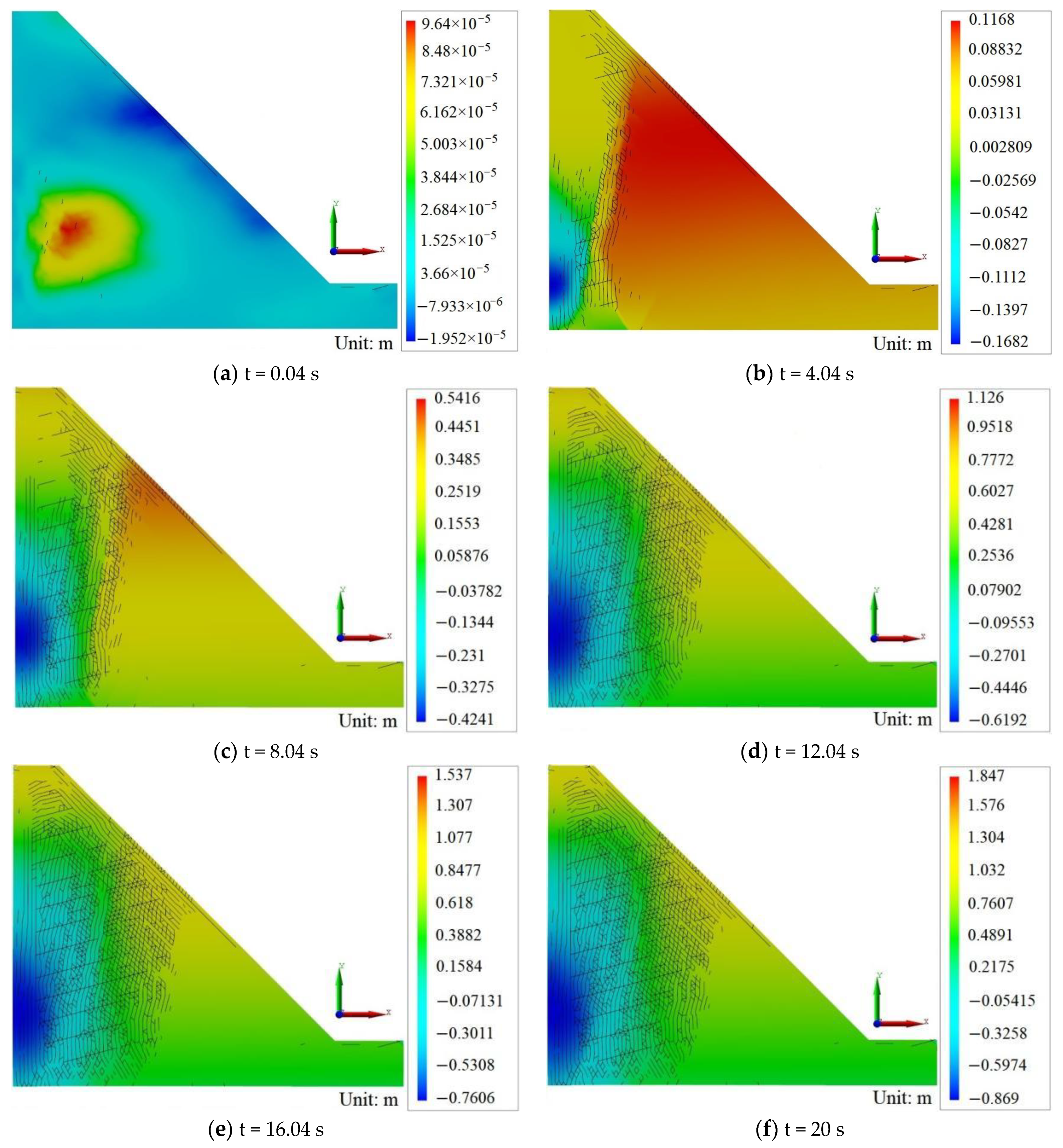
In addition, the shallow slope was further reinforced by secondary grouting, and the displacement distribution of Case 3 under earthquake action is shown in Figure 10. In Figure 10, the deformation of the hilltop area is the largest, and the maximum displacement is approximately 2.047 m, which indicates that the slope crest area is a dangerous area and should continue to be reinforced. For this reason, the slope top is locally reinforced three times. The displacement distribution of Case 4 is shown in Figure 11. In Figure 11, damage deformation occurs at the slope toe first, and the maximum displacement occurs in the slope surface area, which is about 1.89 m. This indicates that the slope toe and crest are the potentially dangerous areas. The slope toe and slope surface in Case 4 are locally reinforced, and the displacement distribution of Case 5 is shown in Figure 12. A comparative analysis of Cases 1–5 shows that the maximum displacement of Case 5 increases significantly. This indicates that local reinforcement should be controlled within a certain number of times, and that constant reinforcement is not beneficial to the stability of the slope, which is also an important principle of inaccurate reinforcement. In order to compare the effect of local precision reinforcement and integral reinforcement, the displacement distribution of Case 6 after integral reinforcement is shown in Figure 13. Figure 13 shows that the maximum displacement of the slope occurs at the slope crest and surface, and the maximum displacement is about 1.847 m, which is similar to the reinforcement effect of Case 4. This phenomenon suggests that the effect of three local precise reinforcements is similar to the overall reinforcement effect. This further illustrates the feasibility, efficiency and economy of local precise reinforcements of the slope.

3.2. Dynamic Response Characteristics of the Partially Reinforced Slope

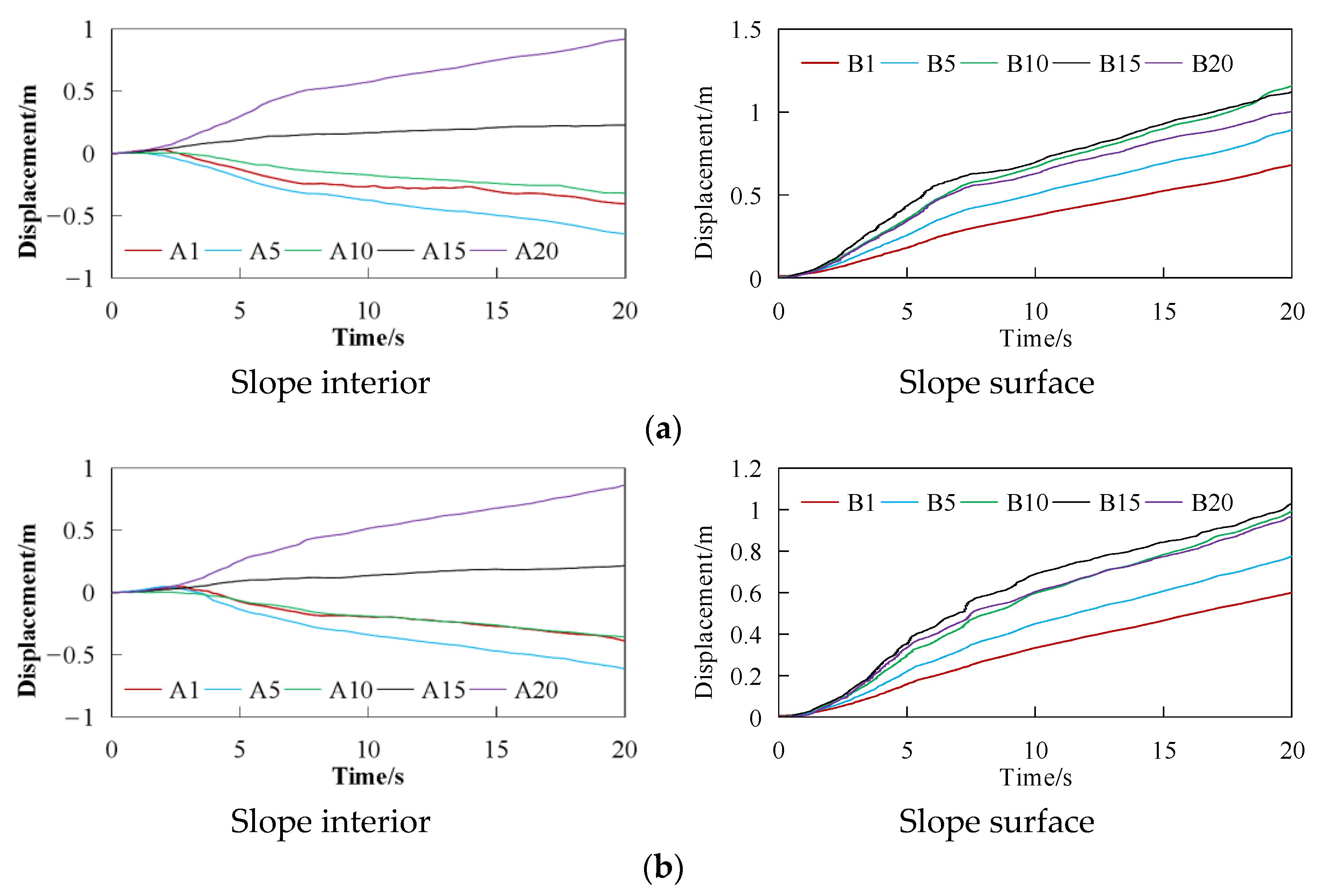
The failure of complex slopes is a gradual evolution process, which has the characteristic of being a gradual, cumulative damage evolution. In order to study the feasibility of the local precise reinforcement method of slopes under earthquake action, the three schemes of unreinforced, local precise reinforcement and overall reinforcement were compared and analyzed. The stability change characteristics of several models after reinforcement were discussed. Taking Case 1 (unreinforced model) and Case 3 (shallow local reinforcement of shallow slope surface) as examples, the displacement and acceleration time histories within the model and on the surface are shown in Figure 14 and Figure 15. Figure 14 shows that the peak ground displacement (PGD) in the slope and on the slope surface decreases to a certain extent after Case 3 is partially strengthened. Figure 15 shows that the peak ground acceleration (PGA) in the slope and on the slope surface decreases to a certain extent after Case 3 is partially reinforced. This indicates that the dynamic deformation of the slope decreases after local reinforcement and the reinforcement effect is better.

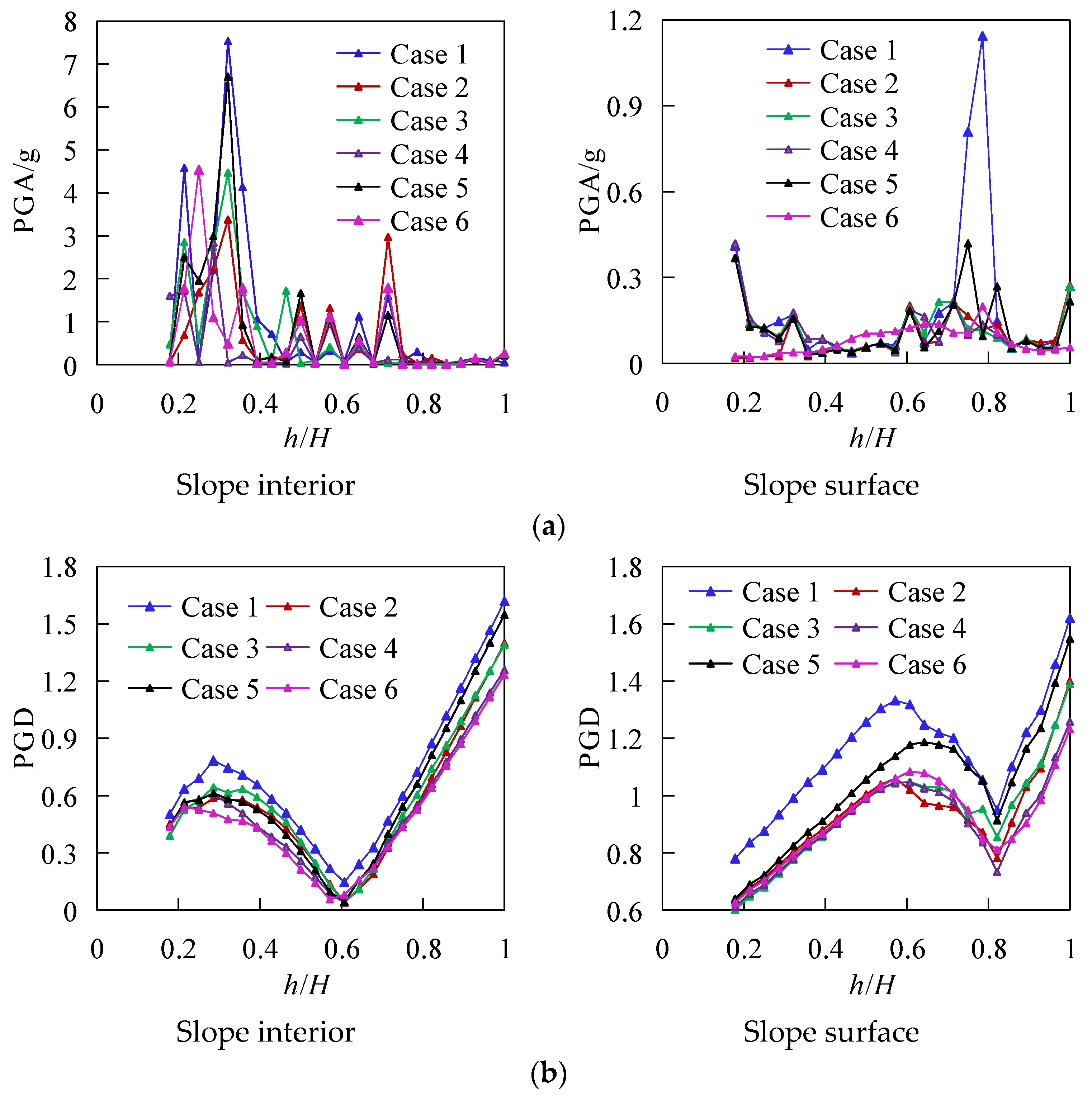
In Figure 16a, through the analysis of PGA changes in the slope interior and at the slope surface, it can be found that PGA presents irregular change characteristics. This is because there are many refraction and reflection effects when the seismic wave passes through the slope body, which leads to the extremely complicated propagation characteristics of the seismic wave in the slope, and then makes the PGA change characteristics in the slope very complicated. By comparing Cases 1–6, it was found that PGA of different models has obvious changes with the change of elevation characteristics. This indicates that local reinforcement and overall reinforcement change the distribution characteristics of the dynamic acceleration amplification effect of slope. In Figure 16b, through the analysis of PGD, it can be seen that the variation trend of PGD of different models is similar in the slope and the slope surface. On the whole, it increases first and then decreases, and then increases in the end. On the whole, PGD on the slope surface increased first, then decreased and finally increased. In general, PGD increases as the elevation increases, reaching its maximum value at the slope crest. By comparing the PGD of different slope models, it was found that local and overall reinforcement did not significantly change the variation trend of PGD.

In order to further explore the beneficial effects of local precise reinforcement, the PGD and PGA of the slopes under different reinforcement conditions were compared and analyzed, as shown in Figure 16. Figure 16 shows that in the slope model (Case 1) without reinforcement under earthquake, the PGD in the slope interior and at the slope surface is much larger. Without reinforcement, deformation and failure are easy to occur first at the slope toe, and the PGD of Case 2 decreases rapidly after partial reinforcement of the slope foot, which indicates that partial reinforcement of the slope has a good effect. However, for Case 2, the slope surface displacement and acceleration amplification effect are the largest. For the shallow surface slope reinforcement (Case 3), the PGD and PGA of Cases 2–3 are similar on the whole. According to the loading ground motion analysis, the slope crest area of Case 3 is prone to instability and failure. Further, the slope crest area of Case 3 is reinforced by grouting (Case 4). Compared with Case 3, PGD and PGA of Case 4 were further reduced on the whole. According to the ground motion analysis of Case 4, the slope surface and the slope toe are prone to damage, and further grouting reinforcement is carried out in this area (Case 5). However, compared with Case 4, the PGD and PGA of Case 5 increased to a certain extent. This shows that the local precision reinforcement method is not always the optimal strategy. However, in a certain number of initial reinforcements, local precision reinforcement has better applicability. When the number of reinforcements increases, there will be excessive reinforcement engineering problems, which not only wastes manpower and material resources, but also weakens the reinforcement effect. In addition, compared with the local reinforcement, the overall reinforcement scheme is Case 6. The PGA and PGD of Case 6 inside the slope are smaller than that of Case 1 on the whole, which indicates that the overall reinforcement has a certain beneficial effect. PGA and PGD of Case 6 and Case 2 are similar, indicating that the effect of local reinforcement is close to that of global reinforcement. This shows the feasibility of local precision reinforcement, which can not only improve the economy, but also improve the prevention efficiency of slope disaster.

Moreover, the ratio of PGA (PGD) of the reinforced models (Case 2–6) to that of the unreinforced model (Case 1) is shown in Figure 17. Figure 17a shows that the PGA ratio of Case 6/Case 1 is significantly greater than that of other models, that is, the acceleration amplification effect after the overall reinforcement is significantly greater than that of the local reinforcement model. This indicates that the dynamic stability of the integral reinforcement is less than that of the local reinforcement, which indicates that the effect and feasibility of the local reinforcement are better. Figure 17b shows that the PGA ratio of Case 6/Case 1 is larger or similar to other models on the whole, indicating that the dynamic stability of the slope after overall reinforcement is less than or close to that of the local reinforcement model. This further shows that local reinforcement is effective and feasible.

3.3. Damage State Assessment of the Partially Reinforced Slope

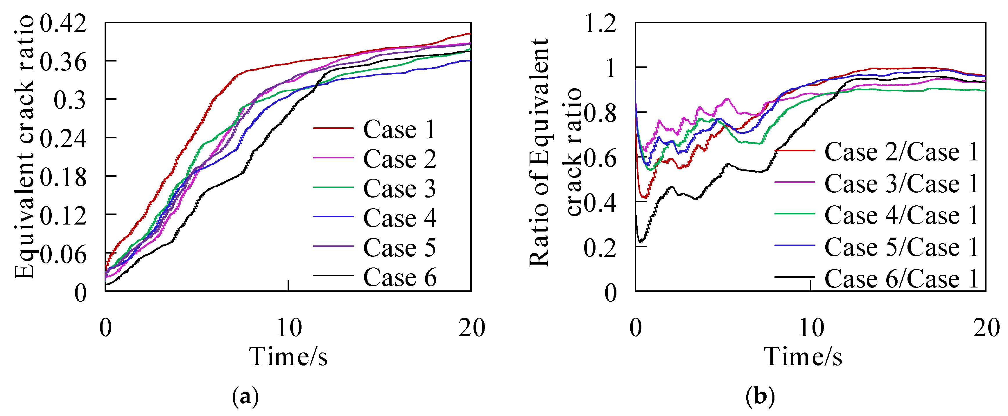
To investigate the stability of slopes, the equivalent crack ratio (R) is used to characterize the slope failure degree, as follows [32]:

$$R=\frac{S_1}{S_2}.$$

(6)

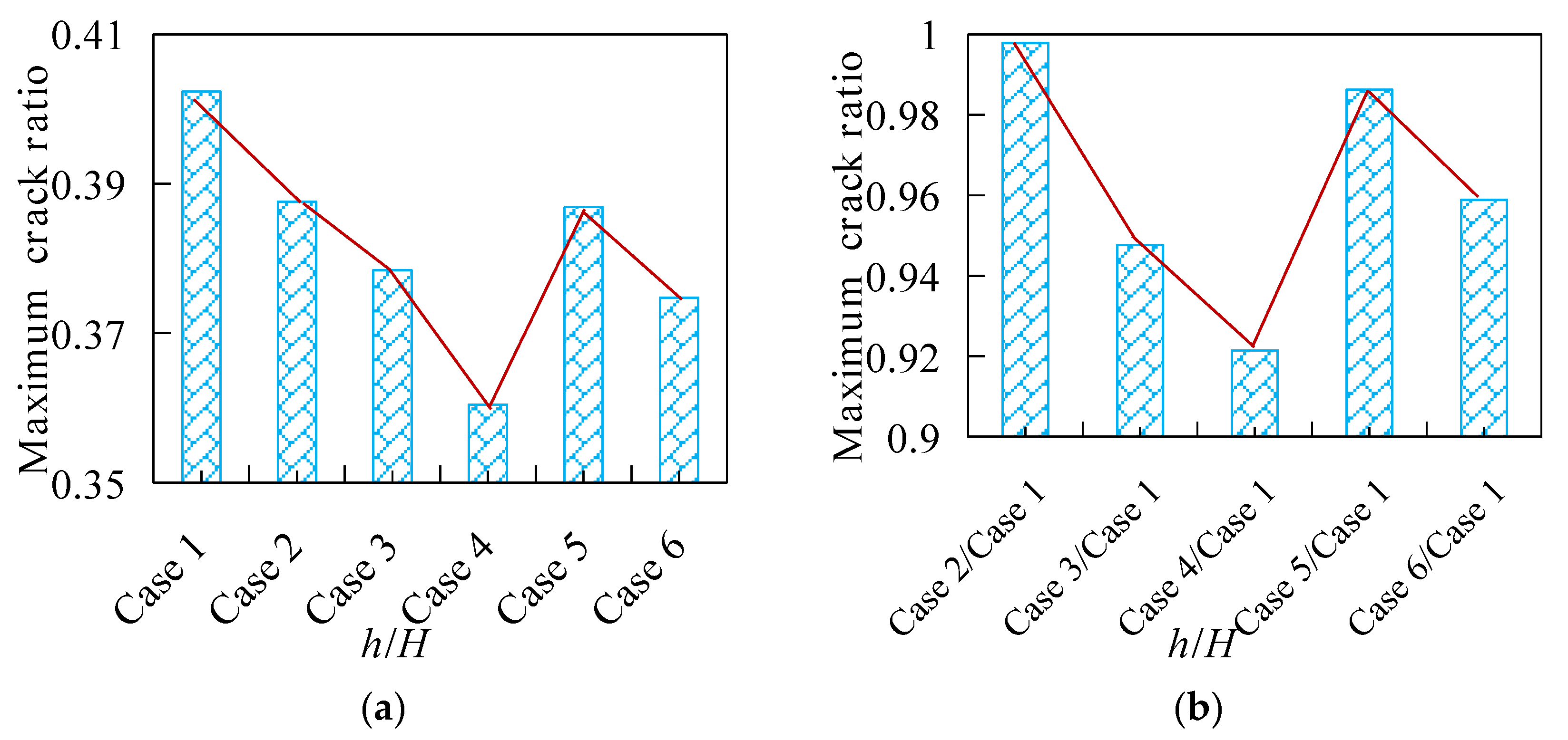
where S₁ is the cumulative value of the product of the spring damage factor and the area, and S₀ is the total contact area of the blocks. The equivalent cracks of different models are shown in Figure 18a. Figure 18a shows that, with the duration of ground motion, the equivalent crack ratio of the slope increases first and then gradually tends to be stable. The rapid increase segment of the unreinforced model Case 1 is 0–7.4 s. After reinforcement, the equivalent crack ratios of the models in Cases 2–6 rapidly increased, with segments of 0–11.6 s, 0–9.6 s, 0–10.5 s, 0–11.5 s and 0–11.8 s, respectively. It can be seen that, after reinforcement, the equivalent crack ratios of the models in Cases 2–6 are rapidly increasing segments that have a backward phenomenon on a time scale. In other words, the slope after reinforcement is less prone to damage, and the duration of the rapid damage stage of Case 6 after overall reinforcement is similar to that of the local reinforcement models in Cases 2–5. This indicates that the beneficial effects of local reinforcement and overall reinforcement on the occurrence time and degree of slope damage are similar. The maximum equivalent crack of the different models is shown in Figure 19a. The ratio of the equivalent crack ratio of the reinforced model to that of the unreinforced model and its maximum value change are shown in Figure 18b and Figure 19b. Figure 19 shows that the maximum equivalent crack ratio after reinforcement decreases in the model, while the maximum equivalent crack ratio of Case 5 increases to a certain extent. This indicates that the local precision reinforcement has a good effect and good applicability within a certain number of initial reinforcement (≤3). When the number of reinforcement (≥4) increases, the reinforcement effect will weaken.

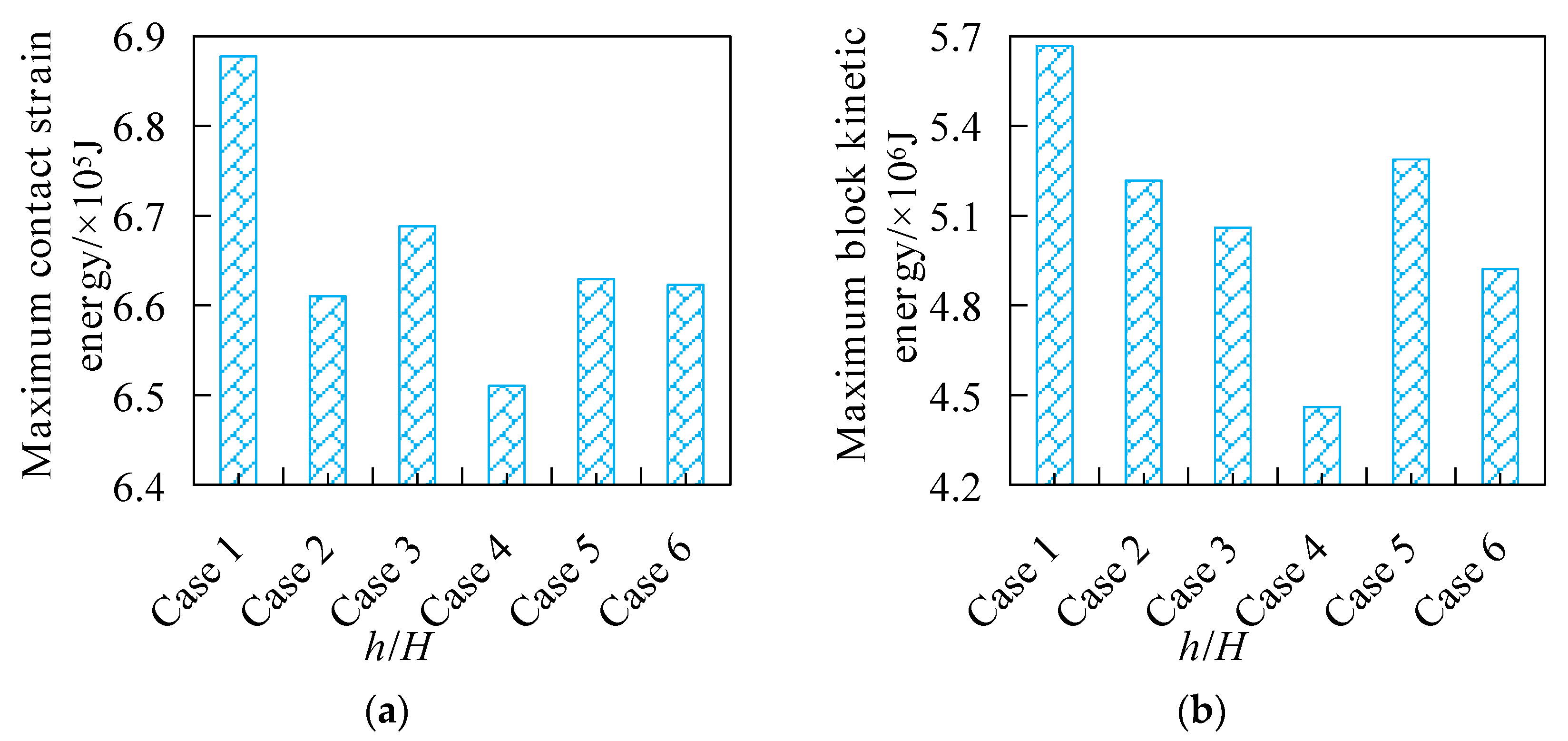
In addition, in order to further explore the effect of the local precise reinforcement method and the global reinforcement method, the contact strain energy and block kinetic energy of different models are shown in Figure 20. The maximum contact strain energy and block kinetic energy of the slope are shown in Figure 21. Figure 20a and Figure 21a show that with the increase in ground motion duration, the contact strain energy between slope blocks gradually increases, and gradually becomes stable after t = 10 s. On the whole, the contact strain between blocks of unreinforced in model Case 1 is the largest, and the overall reinforcement in Case 6 is close to the local precision reinforcement model in Cases 2–5, indicating that the effect of the local precision reinforcement is close to that of the overall reinforcement. In addition, Figure 20b and Figure 21b show that the kinetic energy of the slope blocks is mainly concentrated at t = 3–10 s, which indicates that slope deformation and failure mainly occur in this period. Meanwhile, Case 1 has the largest block kinetic energy, and the kinetic energy of Case 6 and Cases 2–5 is similar, indicating that the effect of local precision reinforcement is similar to that of overall reinforcement.

4. Discussion

In terms of the slope failure process, it is an evolutionary process of gradual failure from local damage accumulation to large-scale sliding failure. The slope reinforcement in the past is characterized by excessive reinforcement. This work provides a new idea for the field reinforcement application of complex slopes, emphasizing that it provides a feasible scheme for the precise reinforcement of complex slopes on the basis of refined numerical simulation analyses. The feasibility and economy of the method are also discussed, which provides a basis for the design of the seismic reinforcement of slopes. According to a series of numerical simulation analyses, it can be found that the effect of Case 4 (third local reinforcement) is similar to that of Case 6 (holistic reinforcement). This shows that local precise reinforcement is effective and feasible, but it is based on the accurate analyses of the evolution process of slope earthquake damage. In the actual engineering application, the analysis should be combined with the specific engineering situation, and the specific implementation plan mainly includes the following steps. Firstly, the slope topography, geomorphology, formation lithology and other information are obtained through detailed field investigation. Secondly, UAV aerial survey is used to obtain slope elevation, image and 3D terrain data. Thirdly, professional aerial photogrammetry software is used to analyze and process the data obtained by UAV and reconstruct the slope three-dimensional model. Then, combined with the detailed field investigation data, the 3D geological model of the slope is established. Then, based on the 3D geological model of the slope, the numerical simulation method is used to establish the same numerical model as the actual slope, to simulate the slope instability process and instability mode. The initial region of slope failure and the failure region of the large deformation stage in the process of instability are determined, and it is listed as a potentially dangerous rock mass and a key area of concern. Then, an appropriate reinforcement structure is adopted to strengthen the initial failure area and large deformation area. Finally, numerical simulation is used to compare the economy, reliability and practicability of precise reinforcement and overall reinforcement of the slope in key areas. This method deeply clarifies the principle and implementation method of the precise reinforcement of the slope, greatly improves the precision, reliability, practicability and economy of slope deformation control and has a wide application prospect in the field of civil engineering and geological disaster prevention.

5. Conclusions

The CDEM numerical simulation is used to discuss the local precise reinforcement and overall reinforcement effects of anti-dip rock slopes subjected to earthquakes. Some main conclusions can be drawn as follows:

• The local precision reinforcement method for the seismic damage of slopes is proposed, and the main content of the local precision reinforcement method is expounded. To find out the distribution and evolution characteristics of the seismic damage of slopes under earthquakes is the premise of reducing the local reinforcement of slopes. The displacement distribution of slopes under earthquakes shows that the displacement of an anti-dip slope is large at the slope toe, crest and shallow surface, and these three areas are the key reinforcement areas. By comparing PGA and PGD of cases, it was found that PGA characteristics of different models changed obviously with the change of elevation, and PGD showed an increase phenomenon as a whole with the increase in elevation. The local and overall reinforcement of slopes changed the distribution characteristics of the dynamic acceleration amplification effect of slopes, but did not significantly change the variation trend of PGD.
• The local precision reinforcement method does not always carry out infinite reinforcement, but should strictly control the local precision reinforcement times of slopes combined with the actual situation. When the number of reinforcements increases, the engineering problem of excessive reinforcement will occur, which not only wastes manpower and material resources, but also weakens the reinforcement effect. The maximum displacement from Case 1 to Case 4 of the slope decreases gradually, while the maximum displacement of Case 5 increases rapidly. This indicates that the first three times local precise reinforcement is performed the effect is better, but when local reinforcement is performed more than three times, the reinforcement effect of the slope gradually becomes worse.
• The dynamic response and seismic damage characteristics of different local precise reinforcement schemes and overall reinforcement schemes are compared and analyzed. Based on the analysis of the PGA, PGD, equivalent crack ratio and block energy of the slopes, the dynamic amplification effect decreases obviously after local precise reinforcement. In particular, the dynamic amplification effect and damage distribution characteristics of Case 4 after three times of local grouting reinforcement are similar to those of Case 6 after overall reinforcement. This indicates that the effect of local precision reinforcement is similar to that of integral reinforcement, that is, the local precision reinforcement method has good feasibility and effectiveness.

References

1. Chen, Z.; Song, D.Q.; Dong, L.H. Characteristics and emergency mitigation of the 2018 Laochang landslide in Tianquan County, Sichuan Province, China. Sci. Rep. 2021, 11, 1578. [Google Scholar] [CrossRef] [PubMed]
2. Chen, Z.; Song, D.Q.; Hu, C.; Ke, Y.T. The September 16 2017, Linjiabang landslide in Wanyuan County, China: Preliminary investigation and emergency mitigation. Landslides 2020, 17, 191–204. [Google Scholar] [CrossRef]
3. Hakim, W.L.; Rezaie, F.; Nur, A.S.; Panahi, M.; Khosravi, K.; Lee, C.W.; Lee, S. Convolutional neural network (CNN) with metaheuristic optimization algorithms for landslide susceptibility mapping in icheon, south korea. J. Environ. Manag. 2022, 305, 114367. [Google Scholar] [CrossRef] [PubMed]
4. Sakurai, A.; Sato, T.; Murayama, Y. Impact evaluation of a school-based disaster education program in a city affected by the 2011 great east japan earthquake and tsunami disaster. Int. J. Disaster Risk Reduct. 2020, 47, 101632. [Google Scholar] [CrossRef]
5. Yulianto, E.; Utari, P.; Satyawan, I.A. Communication technology support in disaster-prone areas: Case study of earthquake, tsunami and liquefaction in palu, indonesia. Int. J. Disaster Risk Reduct. 2020, 45, 101457. [Google Scholar] [CrossRef]
6. Pang, H.P.; Nie, X.P.; Sun, Z.B.; Hou, C.Q.; Dias, D.; Wei, B.X. Upper bound analysis of 3d-reinforced slope stability subjected to pore-water pressure. Int. J. Geomech. 2020, 20, 06020002. [Google Scholar] [CrossRef]
7. Frydrych, M.; Kacprzak, G.; Nowak, P. Hazard reduction in deep excavations execution. Sustainability 2022, 14, 868. [Google Scholar] [CrossRef]
8. Schwerdt, S.; Mirschel, D.; Hildebrandt, T.; Wilke, M.; Schneider, P. Substitute building materials in geogrid-reinforced soil structures. Sustainability 2021, 13, 12519. [Google Scholar] [CrossRef]
9. Bordoloi, S.; Ng, C. The effects of vegetation traits and their stability functions in bio-engineered slopes: A perspective review. Eng. Geol. 2020, 275, 105742. [Google Scholar] [CrossRef]
10. Blondeau, S.; Gunnell, Y.; Jarman, D. Rock slope failure in the western alps: A first comprehensive inventory and spatial analysis. Geomorphology 2021, 380, 107622. [Google Scholar] [CrossRef]
11. Chen, Z.; Song, D.Q.; Juliev MPourghasemi, H.R. Landslide susceptibility mapping using statistical bivariate models and their hybrid with normalized spatial-correlated scale index and weighted calibrated landslide potential model. Environ. Earth Sci. 2021, 80, 324. [Google Scholar] [CrossRef]
12. Abdekareem, M.; Al-Arifi, N.; Abdalla, F.; Mansour, A.; El-Baz, F. Fusion of remote sensing data using GIS-based AHP-weighted overlay techniques for groundwater sustainability in arid regions. Sustainability 2022, 14, 7871. [Google Scholar] [CrossRef]
13. Ma, K.; Tang, C.A.; Liang, Z.Z.; Zhuang, D.Y.; Zhang, Q.B. Stability analysis and reinforcement evaluation of high-steep rock slope by microseismic monitoring. Eng. Geol. 2017, 218, 22–38. [Google Scholar] [CrossRef]
14. Liu, J.; Chen, Z.H.; Kanungo, D.P.; Song, Z.Z.; Bai, Y.X.; Wang, Y.; Li, D.; Qian, W. Topsoil reinforcement of sandy slope for preventing erosion using water-based polyurethane soil stabilizer. Eng. Geol. 2019, 252, 125–135. [Google Scholar] [CrossRef]
15. Fan, G.; Zhang, J.J.; Qi, S.C.; Wu, J.B. Dynamic response of a slope reinforced by double-row antisliding piles and pre-stressed anchor cables. J. Mt. Sci. 2019, 16, 226–241. [Google Scholar] [CrossRef]
16. Chen, W.; Li, D.B.; Ma, T.; Fu, H.L.; Du, Y.P. Stability analysis of a slope considering two reinforcement processes. Geofluids 2020, 816, 8828747. [Google Scholar] [CrossRef]
17. Wang, F.F.; Shao, J.G.; Li, W.K.; Wang, Y.F.; Wang, L.F.; Liu, H.L. Study on the effect of pile foundation reinforcement of embankment on slope of soft soil. Sustainability 2022, 14, 14359. [Google Scholar] [CrossRef]
18. Li, X.Y.; Qin, Z.P.; Tian, Y.; Zhang, H.W.; Zhao, H.T.; Shen, J.F.; Shao, W.L.; Jiang, G.R.; Guo, X.D.; Zhang, J.S. Study on stability and ecological restoration of soil-covered rocky slope of an abandoned mine on an island in rainy regions. Sustainability 2022, 14, 12959. [Google Scholar] [CrossRef]
19. Zhang, R.; Tang, P.X.; Lan, T.; Liu, Z.J.; Ling, S.G. Resilient and Sustainability Analysis of Flexible Supporting Structure of Expansive Soil Slope. Sustainability 2022, 14, 12813. [Google Scholar] [CrossRef]
20. Zhang, S.; Zhang, G.; Zhang, X.; Chen, L.; Zheng, S. Influences on antislide piles used for slope reinforcement: Numerical simulation based on the soil arching effect. Math. Probl. Eng. 2020, 2020, 7651080. [Google Scholar] [CrossRef]
21. Liu, D.; Hu, X.; Zhou, C.; Xu, C.; Wang, Q. Deformation mechanisms and evolution of a pile-reinforced landslide under long-term reservoir operation. Eng. Geol. 2020, 275, 105747. [Google Scholar] [CrossRef]
22. Meijer, G.J.; Bengough, A.G.; Knappett, J.A.; Loades, K.W.; Nicoll, B.C. In situ measurement of root reinforcement using corkscrew extraction method. Can. Geotech. J. 2018, 55, 1372–1390. [Google Scholar] [CrossRef] [Green Version]
23. Sciegaj, A.; Larsson, F.; Lundgren, K.; Runesson, K. On a volume averaged measure of macroscopic reinforcement slip in two-scale modeling of reinforced concrete. Int. J. Numer. Methods Eng. 2019, 121, 1822–1846. [Google Scholar] [CrossRef]
24. Song, D.Q.; Liu, X.; Huang, J.; Wang, E.Z.; Zhang, J.M. Characteristics of wave propagation through rock mass slopes with weak structural planes and their impacts on the seismic response characteristics of slopes: A case study in the middle reaches of Jinsha River. Bull. Eng. Geol. Environ. 2021, 80, 1317–1334. [Google Scholar] [CrossRef]
25. Du, H.; Song, D.Q. Investigation of failure prediction of open-pit coal mine landslides containing complex geological structures using the inverse velocity method. Nat. Hazards 2022, 111, 2819–2854. [Google Scholar] [CrossRef]
26. Feng, W.; Tang, Y.; Hong, B. Landslide Hazard Assessment Methods along Fault Zones Based on Multiple Working Conditions: A Case Study of the Lixian–Luojiabu Fault Zone in Gansu Province (China). Sustainability 2022, 14, 8098. [Google Scholar] [CrossRef]
27. Solórzano, J.; Morante-Carballo, F.; Montalván-Burbano, N.; Briones-Bitar, J.; Carrión-Mero, P. A Systematic Review of the Relationship between Geotechnics and Disasters. Sustainability 2022, 14, 12835. [Google Scholar] [CrossRef]
28. Shu, H.; Guo, Z.; Qi, S.; Song, D.Q.; Pourghasemi, H.R.; Ma, J. Integrating Landslide Typology with Weighted Frequency Ratio Model for Landslide Susceptibility Mapping: A Case Study from Lanzhou City of Northwestern China. Remote Sens. 2021, 13, 3623. [Google Scholar] [CrossRef]
29. O’Connor, W.; Mider, G.; Lawrence, J.A.; Agar, S.; Mason, P.J.; Ghail, R.; Scoular, J. An Investigation into Ground Movement on the Ventnor Landslide Complex, UK Using Persistent Scatterer Interferometry. Remote Sens. 2021, 13, 3711. [Google Scholar] [CrossRef]
30. Zhang, J.; Li, W.; Ye, S. Stability Analysis of Filled-Slope Reinforced by Frame with Prestressed Anchor-Plates under Static Action. Appl. Sci. 2023, 13, 1615. [Google Scholar]
31. Wang, J.; Liu, P.; Si, P.; Li, H.; Wu, F.; Su, Y.; Long, Y.; Cao, A.; Sun, Y.; Zhang, Q. Three-Dimensional Stability Analysis of Ridge Slope Using Strength Reduction Method Based on Unified Strength Criterion. Appl. Sci. 2023, 13, 1580. [Google Scholar] [CrossRef]
32. Feng, C.; Li, S.H.; Hao, W.H.; Ge, W. Numerical simulation for penetrating and blasting process of epw based on cdem. J. Vib. Shock 2017, 36, 11–18. [Google Scholar]
33. Zhang, Q.L.; Zhi, Z.H.; Feng, C.; Cai, Y.C.; Pang, G.H.; Yue, J.C. Investigation of concrete pavement cracking under multi-head impact loading via the continuum-discontinuum element method. Int. J. Impact Eng. 2020, 135, 103410.1–103410.13. [Google Scholar] [CrossRef]
34. Wang, C.W.; Liu, X.L.; Song, D.Q.; Wang, E.Z.; Zhang, J.M. Numerical investigation on dynamic response and failure modes of rock slopes with weak interlayers using continuum discontinuum element method. Front. Earth Sci. 2021, 9, 791458. [Google Scholar] [CrossRef]
Figure 1. Geographical location of the study area.
Sustainability 15 02490 g001
Figure 2. Geomorphology and engineering geological profile of the anti-dip slope: (a) Geomorphology; (b) engineering geological profile.
Sustainability 15 02490 g002
Figure 3. Comparison of different numerical methods principle: (a) FEM; (b) DEM; (c) CDEM.
Sustainability 15 02490 g003
Figure 4. CDEM contact relationship.
Sustainability 15 02490 g004
Figure 5. Schematic diagram of CDEM calculation process.
Sustainability 15 02490 g005
Figure 6. Numerical model and measuring points layout of the anti-dip slope: (a) model mesh; (b) measuring points.
Sustainability 15 02490 g006
Figure 7. Seismic wave loading in the numerical model.
Sustainability 15 02490 g007
Figure 8. Displacement distribution of Case 1 (slope without reinforcement) under earthquake.
Sustainability 15 02490 g008
Figure 9. Displacement distribution of Case 2 (slope after the first grouting reinforcement at the slope toe).
Sustainability 15 02490 g009
Figure 10. Displacement distribution of Case 3 (slope after the second grouting reinforcement at the shallow slope surface).
Sustainability 15 02490 g010
Figure 11. Displacement distribution of Case 4 (slope after the third grouting reinforcement at the slope crest).
Sustainability 15 02490 g011
Figure 12. Displacement distribution of Case 5 (slope after the fourth grouting reinforcement at the shallow slope surface and slope toe).
Sustainability 15 02490 g012
Figure 13. Displacement distribution of Case 6 (slope after the integral reinforcement).
Sustainability 15 02490 g013
Figure 14. Displacement time history: (a) Case 1; (b) Case 3.
Sustainability 15 02490 g014
Figure 15. Acceleration time history: (a) Case 1; (b) Case 3.
Sustainability 15 02490 g015
Figure 16. Amplification effect of the slopes changes with elevation under different reinforcement conditions: (a) PGA; (b) PGD.
Sustainability 15 02490 g016
Figure 17. Ratio of amplification effect of the slope under different reinforcement conditions: (a) PGA; (b) PGD.
Sustainability 15 02490 g017
Figure 18. Variation of the slope damage characteristics: (a) equivalent crack ratio; (b) ratio of crack ratio under reinforcement conditions to that before reinforcement.
Sustainability 15 02490 g018
Figure 19. Variation of the maximum equivalent crack ratio of Cases 1–6: (a) maximum equivalent crack ratio; (b) ratio of crack ratio under reinforcement conditions to that before reinforcement.
Sustainability 15 02490 g019
Figure 20. Variation of energy of blocks in the slope: (a) contact strain energy; (b) kinetic energy.
Sustainability 15 02490 g020
Figure 21. Variation of maximum energy in the slope: (a) contact strain energy; (b) block kinetic energy.
Sustainability 15 02490 g021