Article

Improving NoSQL Spatial-Query Processing with Server-Side In-Memory R*-Tree Indexes for Spatial Vector Data

1
Faculty of Geography, Yunnan Normal University, Kunming 650500, China
2
Information Center, Department of Natural Resources of Yunnan Province, Kunming 650224, China
*
Author to whom correspondence should be addressed.
Sustainability 2023, 15(3), 2442; https://doi.org/10.3390/su15032442
Submission received: 10 November 2022 / Revised: 25 January 2023 / Accepted: 28 January 2023 / Published: 30 January 2023
(This article belongs to the Special Issue Geographic Information Science for the Sustainable Development)

Abstract

:
Geospatial databases are basic tools to collect, index, and manage georeferenced data indicators in sustainability research for efficient, long-term analysis. NoSQL databases are increasingly applied to manage the ever-growing massive spatial vector data (SVD) with their changeable data schemas, agile scalability, and fast query response time. Spatial queries are basic operations in geospatial databases. According to Green information technology, an efficient spatial index can accelerate query processing and save power consumption for ubiquitous spatial applications. Current solutions tend to pursue it by indexing spatial objects with space-filling curves or geohash on NoSQL databases. As for the performance-wise R-tree family, they are mainly used in slow disk-based spatial access methods on NoSQL databases that incur high loading and searching costs. Therefore, performing spatial queries efficiently with the R-tree family on NoSQL databases remains a challenge. In this paper, an in-memory balanced and distributed R*-tree index named the BDRST index is proposed and implemented on HBase for efficient spatial-query processing of massive SVD. The BDRST index stores and distributes serialized R*-trees to HBase regions in association with SVD partitions in the same table. Moreover, an efficient optimized server-side parallel processing framework is presented for real-time R*-tree instantiation and query processing. Through extensive experiments on real-world land-use data sets, the performance of our method is tested, including index building, index quality, spatial queries, and applications. Our proposed method outperforms other state-of-the-art solutions, saving between 27.36% and 95.94% on average execution time for the above operations. Experimental results show the capability of the BDRST index to support spatial queries over large-scale SVD, and our method provides a solution for efficient sustainability research that involves massive georeferenced data.

1. Introduction

In recent years, the development of communication, the Internet of Things (IoT), and big data technology have brought us into the smart planet era [1]. Increasing data acquisition methods and extensive spatial applications such as smart city [2], augmented reality (AR) [3], and natural hazard risk assessments [4] have prompted massive, multi-format geospatial data. Spatial queries can be described as finding qualified spatial objects from such spatial datasets. They are basic geographical information system (GIS) operations for geospatial analysis, such as overlay analysis [5,6] and spatial join operations [7,8].
Spatial databases provide data storage and indexing components for spatial queries. Facing the ever-growing volume and number of data types, conventional relational spatial databases struggle to meet the requirement of fast, scalable, and high-concurrency spatial applications [9,10,11]. The major overhead in SQL databases includes ACID (Atom, Consistency, Isolation, Durability) transactions [12], communication costs between the application and DBMS (database management system) [13], and some OLTP (online transaction processing) overhead components [13]. NoSQL (Not-only SQL) databases reduce the overhead by jettisoning the ACID transactions and show some widely-accepted features such as horizontal scaling, fast reading/writing support, high availability, and high concurrency [14]. GIS database-related studies are one of the general topics in GIScience [15]. In the last two decades, there has been a surge in interest on developing spatial data stores based on NoSQL databases for efficient spatial information processing [10].
Spatial indexes are core components in spatial databases since they can roughly filter objects that do not meet the spatial constraints to accelerate spatial-query processing [16]. NoSQL databases are originally designed for handling the vagaries of Internet-size workloads [12] for web search [17], social media [12], e-commerce [18], etc. Vast efforts have been made to craft a spatial index to extend NoSQL databases for spatial data management. The most popular way is to use space-specific [19] or space-driven [20,21] spatial indexes to map or transform the two-dimensional or higher-dimensional spatial data into one-dimensional space. These spatial indexes, such as space-filling curves (SFC) and geohash, adopt a regular, hierarchical, space-split pattern and allocate objects to the elementary cells, which endows them with excellent updating performance. However, the regular space-split pattern gives little consideration to the spatial distribution of objects and brings some drawbacks including relatively high approximation error [22], allocation for cross-cell geometries [22], and high cost for lexicographic range mapping [19]. In query processing, these drawbacks degrade the performance of the data-specific spatial indexes compared with those spatial indexes concerning the distributions of spatial objects.
R-tree [23] and its variations [24,25] are data-specific [19] or data-driven [21], depth-balanced spatial indices, and have been widely used in SQL databases, such as Oracle [26], PostGIS, as well as in NoSQL databases [10]. R*-tree index is known as the most performance-wise R-tree variant in retrieving performance but rarely employed in NoSQL databases. All pointers of nodes in an R-tree index are actual addresses to magnetic disk locations [21,27]. On the other hand, it is impossible for most databases to cache R-trees in the main memory while storing massive SVD [28]. In most cases, the R-tree family was used as a disk-based spatial index. In NoSQL databases, the R-tree was usually flattened as basic data elements in a NoSQL table, such as documents in MongoDB [27] and rows in HBase [29,30], or stored in an external storage to support spatial-query processing for NoSQL databases [31,32]. Such disk-based usage of the R-tree family suffers from notable latency in slow index loading and searching on disk. Memory-based parallel computing technologies such as Spark provide some inspirations for accelerating spatial queries with distributed in-memory R-tree indexes; some solutions have verified the efficiency of in-memory usage of R-tree family [8,33,34]. However, if we plan to provide efficient spatial-query services with Spark for large-scale SVD, in-memory capability can become a bottleneck since keeping both data and index in memory is quite expensive.
In this paper, we present a BDRST index based on server-side in-memory R*-trees for efficient spatial-query processing of massive spatial vector data on HBase. Different from conventional disk-based R-tree usage or Spark-based spatial-query processing, our method moves R*-tree indexes to HBase server-side computing resources by storing a local serialized R*-tree instance in each region of the HBase SVD table. With our elaborately implemented server-side parallel processing framework based on an HBase coprocessor, R*-tree indexes can be instantly loaded into memory and searched for parallel query processing. To the best of our knowledge, the proposed method is a novel idea for efficient spatial-query processing on NoSQL database with the following merits: (1) fast query response; (2) agile scalability; (3) integrated and simple storage schema for R*-trees and SVD.
The contributions of this paper are as follows:
(1) Designing a distributed index structure for SVD based on R*-trees. R*-trees are balanced and localized into regions of the HBase table along with SVD for fast server-side loading and spatial-query processing;
(2) Implementing a parallel processing mechanism based on an HBase coprocessor for server-side parallel loading of localized R*-trees, spatial-query processing, and query-based custom processing;
(3) Using real-world datasets, we designed and conducted a series of experiments to evaluate the performance of the method, including index building, index quality, spatial-query processing, and scalability as the query extent expands. We compared the method with the state-of-the-art NoSQL spatial-query processing tool Geomesa.
The remainder of the paper is structured as follows: Section 2 reviews the related work. Section 3 elaborates our proposed BDRST indexing method and the implementation on HBase. In Section 4, the experimental analysis is illustrated with comprehensive evaluation metrics. Finally, we present conclusions and prospects for future research in Section 5.

2. Related Work

2.1. Sustainability in Geospatial Databases

Sustainability is widely accepted as the definition of sustainable development in the Brundtland Report, which is the ability to fulfill present development without compromising the development of future generations [35]. To analyze or assess sustainability is to find the dynamic, complex, and composite data relationship among human activities and natural ecosystems [36]. Since human-nature interactions happen in the geographic space, the data indicators in sustainability research are georeferenced [37]. The geographical properties of these indicators, such as regionalities and locations, are essential dimensions for sustainability research [38,39].
In recent years, data science has driven increased attention as a promising solution in sustainability analysis. Many studies organize such multi-scale and multidimensional relevant data in a geospatial or georeferenced database, for fast retrieval, efficient storage, flexible analysis, and data mining [36,37,38]. Geospatial databases can collect, store, and index large-scale georeferenced data for long-term analysis. Some studies collect multi-temporal and multi-source geo-tagged data sets and generate a land use land cover (LULC) database. Based on that, researchers can easily access the target information and use GIS analysis tools for ecosystem service research [40,41], pasture dynamics research [42], etc. There is additional research using geospatial databases in sustainable agroecosystems [37], digitalized aqua farming [43], and sustainable foods [44].
Another research topic in geospatial databases and sustainability is Green Information Technology (Grenn IT). Green IT focus on reducing the direct impacts of IT activities on the environment [37]. More specifically, Green IT requires energy-efficient or energy-saving hardware and software approaches to mitigate power consumption [45] for sustainable information services. Regarding the cost of data querying and transmission, most Green IT solutions concentrate on improving the energy efficiency of database servers [37,45] and network components [46]. According to previous studies in [45], query optimizations in SQL/NoSQL databases such as the use of indexes, row caching, and data compaction can achieve significant improvements in energy efficiency without performance degradation. The general principle for energy efficiency is to reduce redundant disk accesses [47] and data communication costs in networks [46]. If we perform a query, the most ideal scenario is that the database can directly find the qualified objects without accessing any irrelevant objects or repeated communication with the client. The whole query processing performs with only a one-time communication and returns the results to the client. Geospatial databases also follow the above optimizing strategy in consideration of both query performance and energy efficiency. According to the spatial access method, if an optimization reduces redundant accesses and communication costs, such optimization can also improve the query-processing performance.

2.2. NoSQL Databases and HBase

NoSQL databases were created and evolved with the development of the internet, cloud computing, and various big-data applications with high user load, data load, scale agility, and computational scalability [12]. The definition of NoSQL is mostly accepted as “Not-only SQL” since NoSQL databases sacrifice the ACID transactional properties for higher read/write performance [13,14]. To deal with voluminous data, NoSQL databases can horizontally split, store, and replicate the data over different servers. This sharding feature also brings NoSQL databases high availability as data are replicated among different nodes [48]. Although some SQL databases also support shard data over multiple nodes on the provisos that use small-scope operations and transactions [14], such as MySQL Cluster, their scaling size is relatively small compared with NoSQL databases [14], and multi-node operations must be avoided for scalable performance [14,49].
NoSQL databases mainly introduce four types of data models: key-value, document, column-oriented (wide-column), and graph models. The common NoSQL data stores based on these data models are reviewed in [10,13,14]. HBase is a column-oriented, open-source, versioned, distributed NoSQL database with high availability, scalability, and reading/writing performance. The HBase project is written in Java and modeled after Google Bigtable [17]. As a column-oriented data store, the basic data model of HBase consists of rows and columns. HBase rows are split across nodes through sharding on the one-dimensional primary key that sorts, splits, and indexes with native B-trees [14]. Hence, row operations such as get and filter in HBase are atomic to avoid redundant access to every node. HBase also indexes columns and compresses data to reduce I/O cost. However, the B-trees in HBase cannot organize two-dimensional or higher-dimensional spatial objects.
Another component for NoSQL database high performance is the server-side coprocessing framework (SSCP) that resembles the stored-procedure in SQL databases. SSCP enables NoSQL databases to run custom codes at each region or tablet on the server-side where the computation can operate on the data directly without communication overheads. SSCP provides a very flexible model for building distributed services and inherit some characteristics of NoSQL databases such as automatic scaling, load balancing, and request routing for applications. Typical SSCP frameworks include Accumulo Iterators, HBase Coprocessor, Aerospike User-defined Functions, CouchDB Views, etc. Recent advancements in the SSCP-based secondary index mechanism and transaction tools such as Apache Phoenix provide insight into improving NoSQL spatial-query processing. SP-Phoenix extends Phoenix with geohash-based spatial indexes for massive spatial points management on HBase [50]. Open-source spatial tools for NoSQL databases such as Geomesa [19] and its extensions [18,51] improve the spatial-query efficiency based on their space-filling-curve indexes with an SSCP framework. Some studies have designed SSCP-based indexes for meteorological data [52] and traffic data [53].
In HBase, the SSCP is named as an HBase coprocessor that is modeled after Google Bigtable’s coprocessor implementation [17]. HBase coprocessor contains two components: observers and endpoints that resemble the triggers and stored procedures in SQL databases. More specifically, observers are triggered either before or after a specific base HBase activity or event occurs, for instance, to automatically update the total number of the rows in a current region after putting an new HBase row. Endpoints are more powerful since they support complex implementation that runs remotely at the target region or regions. The results from those executions will be returned to the client in a compressed format with the help of Google’s Protocol Buffer to reduce the I/O cost.
Also note that the SSCP utilizes memory from the heap of NoSQL databases nodes, which is relatively much smaller than the memory resources in a Yarn cluster for Spark jobs. Memory-intensive tasks should not run on SSCP to avoid heap overflow on NoSQL database servers.

2.3. R*-Tree and R-Tree Family

Various spatial indexes have been proposed for fast spatial-query processing due to their well-directed access on relevant objects, such as Grid, K-D-B Tree [54], Quadtree [55], the R-tree family [23,24,25], one-dimensional orderings with SFCs, and others. Among them, the R-tree family is the most influential data-driven access method with good retrieval performance. Most instances in the R-tree family employ a hierarchical structure to organize the minimum bounding rectangles (MBRs) of spatial objects. As a performance-wise spatial index, R*-trees [24] are frequently picked to benchmark and compare the performance of new spatial-query processing methods in the literature.
The R*-tree follows the same structure as the R-tree. R*-tree is a height-balanced tree. Each non-root node stores m to M elements that indicate the minimum and maximum number of entries, respectively, where m M / 2 . Entries are in the form of (id, r). In leaf nodes, id is an identifier addressed to the specific spatial object whose MBR is r. In internal nodes, id is a node identifier addressed to a child node, and r records the MBR that encloses all the child nodes. The single node-splitting criteria of the R-tree can cause large rectangles and significantly increase the overlap between nodes. The R*-tree considers four criteria for node splitting: (1) minimization of overlap between r; (2) minimization of the perimeter of r; (3) minimization of the area covered by r; (4) maximization of storage utilization. As Figure 1 shows, the R*-tree applies a heuristic approach to find suitable combinations of these criteria for better performance and establishes a forced reinsertion strategy to rebalance the existing tree and reduce the overlap between neighboring nodes. All these comprehensive optimizations enhance the performance of the R*-tree, especially the retrieval performance.
The searching algorithm of an R*-tree is also the same as the R-trees. It is to downward examine all the nodes in the R*-tree that satisfy the given spatial predicate with the query geometry. For example, finding spatial objects within the given spatial extent or within the distance of the given spot is a spatial query. Conversely, the inserting algorithm in the R*-tree is to allot entries (id, r) to the suitable node upward. If the chosen leaf node is full, it will perform a split operation or a forced reinsertion. The split operation will create a new leaf node that is later inserted in the parent node of the current leaf node. The forced reinsertion is that to pick out entries of the overflowed node and reinsert them to optimize the R*-tree structure. In some cases, both two operations may launch a series of upward chain operations that may reconstruct the whole R*-tree structure.

2.4. Spatial-Query Processing on NoSQL Databases

Spatial vector data are semi-structured or unstructured data as the shape complexities of features are different, and the vertices of geometries vary [56]. NoSQL databases are more suitable for SVD storage than SQL databases as they can directly store SVD in a common format such as GeoJSON, WKT (well-known text), or WKB (well-known binary). Although some NoSQL databases provide native spatial indexes for spatial-query processing, most of them are not well-designed for geospatial data [32] due to the limited spatial data types and query functions [10]. Therefore, vast efforts have been made for building spatial-query processing approaches for NoSQL databases.
The key problem of spatial-query processing on NoSQL databases is to design a proper spatial index which is not merely the core factor for query efficiency, but also closely interrelated with the SVD storage schema. A simple way is to add an external spatial index to NoSQL databases. Accordingly, NoSQL databases only act as storage containers for SVD, and the spatial indices are maintained in another container, such as a file system or a SQL database. In [31], a Hilbert R-tree index for HBase was designed, which is packed with a Hilbert curve and maintained in a Hadoop Distributed File System (HDFS). However, according to their spatial-query processing experiments, the time cost for the index loading was too high. Antares [32] built a distributed index cache for KD-Trees, Quad Trees, and Geohashes over client nodes in a cluster and mapped these nodes with Cassandra data nodes to support parallel spatial-query processing. Theoretically, such solutions enable NoSQL databases to use any developed spatial indexes. However, the separation of the spatial indexes and data incurs higher access overhead for the cross-platform communication, as well as the complex issues in consistency, data security, backup, and concurrent access.
Some NoSQL databases inlay a native R-tree index for spatial queries, such as Couchbase and Neo4j spatial. However, there are some limitations in spatial data types or spatial functions [10]. According to the previous experiment [57], Neo4j spatial was the most time-consuming one in spatial-query processing when compared with MongoDB and PostGIS [57]. Some research aims to provide R-tree support for NoSQL databases by flattening the R-tree as basic data elements in a NoSQL table. [27] flatten the R-tree as documents in MongoDB to manage spatial planar data. [29,30] flatten the R-tree as rows in an HBase table to for spatial-query processing with points or polygons. Using this disk-based R-tree, processing a spatial query is to scan a NoSQL table. As the query range expands, the performance of the scan operation endures a serious degradation from the increasing invalid fragment queries [58,59].
Other literature focuses on extending NoSQL databases for spatial-query processing with a one-dimensional ordering technique. Typical spatial indexes are SFCs such as the Hilbert curve [60,61], Peano/Morton curve [29], XZ-ordering [22], and geohash. They adopt a hierarchical and fixed space division, such as a quadratic split, and encode spatial objects by concatenating the identifiers of their overlapping cells downward. The encoded geohash sequences can be saved as primary keys and form a spatial index or be combined with more attributes for a higher-dimension index (e.g., combining with timestamps for a spatiotemporal indices). NoSQL databases can directly handle such one-dimensional orderings to transform a multidimensional search to table scanning or row filtering. MD-Hbase encodes the positioning data with a Z curve and implements K-D tree and quad-tree indices in HBase [59]. In St-Hbase, the STbHI index has been proposed, which composes terms and Z-ordering values for efficient spatial keyword queries on HBase [62]. PAIRS uses the Z-curve index and implements a geospatial data analytics platform on HBase for fast modeling. In [29], a Z-curve-based storage schema for spatial data storage was designed, which outperformed the quad-tree and R-tree according to their experiments.
XZ-ordering is an optimized Z-ordering based on the Morton curve resolving the high approximation error [22]. It introduces an enlarged overlapping cell to control the approximation error and a sophisticated coding scheme to encode variable-length sequences as integers in an order-preserving manner [22]. Through the above improvements, XZ-ordering has the advantages of resolution insensitivity and better support for polygons. Geomesa [19] and its extensions [18,51] are all based on XZ-ordering a spatial index for NoSQL databases and are very popular in recent LBS applications. However, due to the fixed quadratic space split, the approximation error of the XZ-ordering index remains much higher than the data-driven spatial indexes, which means a more redundant access. Moreover, comparing in-memory indexes, the disk-based scanning over orderings is slower for the I/O cost.

3. Methodology

In this section, we introduce the proposed BDRST indexing approach to provide fast spatial-query processing for HBase. We tackle the problem of high loading and searching cost in NoSQL spatial-query processing based on disk-based R-tree variants. The R*-tree index provides fine-grained spatial retrieve results and reduces the redundant data accesses. Moreover, we implement a server-side parallel spatial-query processing mechanism based on HBase Endpoints to reduce data communication between the client and servers. According to the optimizing principles for sustainability in geospatial databases, the BDRST index and the processing mechanism improve the spatial-query processing performance, as well as energy-efficiency in HBase.

3.1. Application Types

Our method is currently used for processing two typical spatial queries: intersection range query (IRQ), k-nearest neighbor (kNN) query, and the applications based on these two types of spatial queries.
Intersection range query is a common spatial query that returns the spatial objects that intersect the query geometry q. A plain IRQ returns the objects whose MBRs intersect the MBR of the q, while an IRQ with geometry filters only returns the objects whose raw geometries intersect the q.
A k-nearest neighbor query finds the k nearest to the query geometry q, and the spatial objects can be measured by different metrics such as the Euclidean distance, the Manhattan distance, etc. In our case, kNN queries check the actual distance relationships between the raw geometries from the query data set and the q and return precise results.
Since HBase Endpoints are easy to implement and extend, our method is also capable of swiftly extending to spatial applications based on IRQs or kNN queries. We present a common spatial application instance named land-use compliance review (LUCR). LUCR is used to review application plans for compliance with the land-use provisions in laws and regulations. It involves zoning, subdivision, drainage/floodplain, water quality, transportation, environmental review, erosion control, and mitigation and/or protection of protected or heritage trees. LUCR calculates the intersection between the spatial extent of an application plan and the review data, such as natural reserves and crop farmland, and summarizes the area of the intersection. In processing phases, LUCR consists of IRQs, intersection, and statistical analysis.

3.2. Architecture Overview

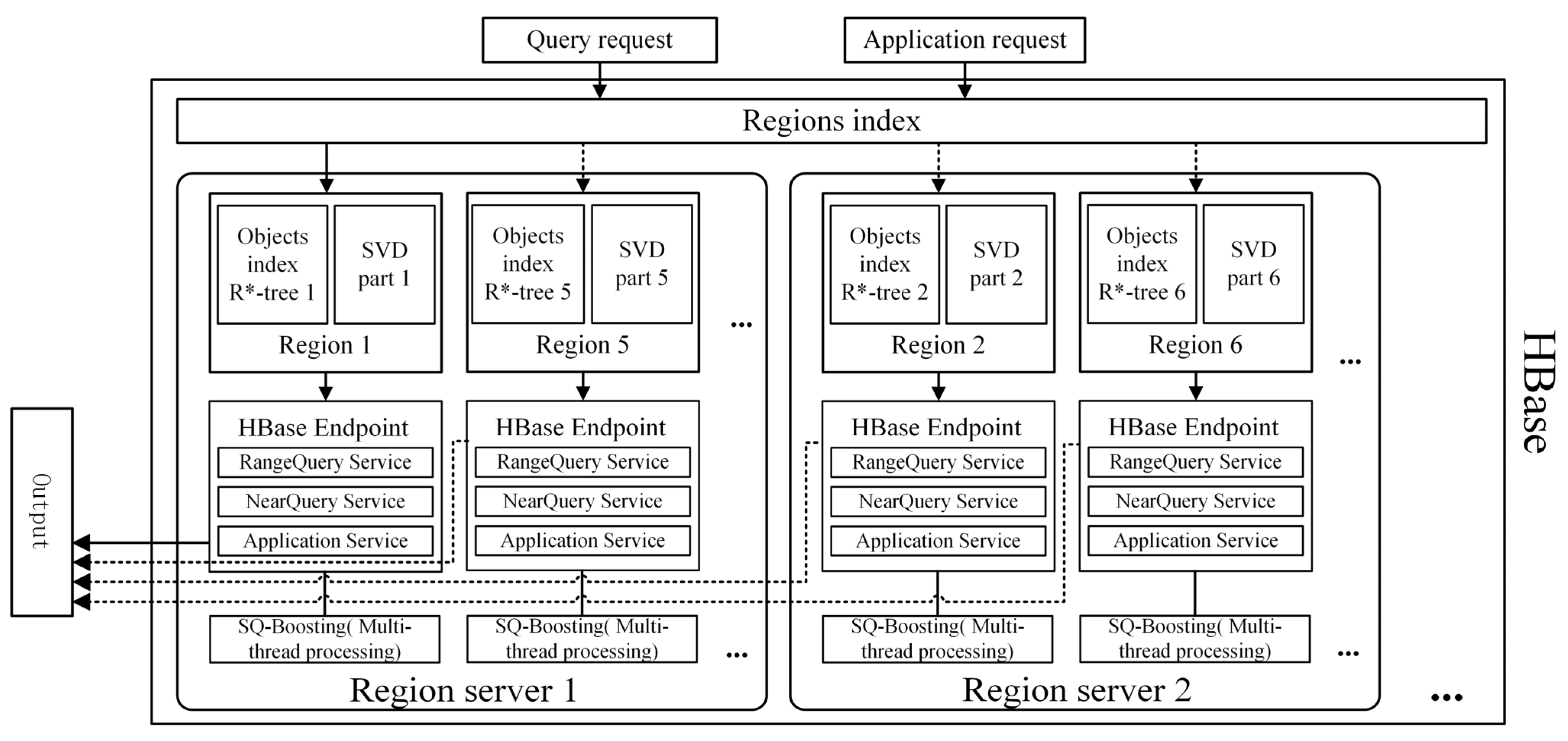
The whole spatial-processing method is solely based on HBase. A BDRST index consisting of the regions index and objects index is proposed and localized along with SVD partitions in regions of an HBase table to avoid cross-platform and cross-table access. As Figure 2 shows, the regions index records the identifiers and spatial extents of regions for region-level filtering. An objects index is an R*-tree in each region to filter the indexed spatial objects. Based on HBase coprocessor interfaces, we implement a parallel processing mechanism for R*-trees real-time loading, data retrieving, query processing, and application in qualified regions on region servers. To further improve the efficiency, a second-stage boosting mechanism (SQ-Boosting) is incorporated as it accelerates each processing task with multi-thread processing.

3.3. SVD Partitioning and Balancing

A tree-like spatial index requires 15% additional storage overhead [63,64], which is also the memory overhead if the index is designed for in-memory usage. To control the overhead, the BDRST index is designed as a two-level spatial index based on distributed R*-trees instead of a single global R*-tree. To reduce the skewness of memory overhead in the parallel loading of R*-trees, we implement an optimized a sort-tile-recursive partitioning (STRP) strategy called adaptive sort-tile-recursive partitioning (ASTRP) to split large-scale SVD into balanced partitions.
The original STR algorithm [65] was proposed as an upward packing algorithm for R-tree construction and currently applied as a spatial data partitioning (SDP) method [7,8,64] since it ensures the spatial clustering in a rectangular shape of the spatial objects in each partition. More importantly, STRP can generate item-balanced partitions where the number of spatial objects in the partitions is almost the same. Hence, the distributed R*-trees built over partitions generated by STRP have nearly the same memory overhead due to the equal capacity.
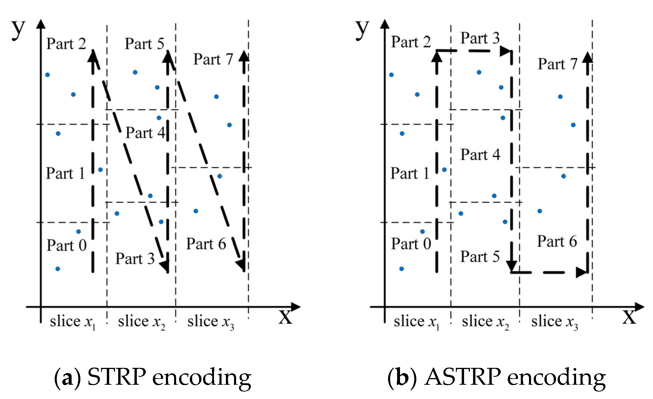
ASTRP follows the main processing steps of STRP. Suppose that we need to split N two-dimensional spatial objects into p partitions. We need to calculate the centroids of each geometry first then later sort them by their x coordinates from the left to right. Then, ASTRP will slice the sorted objects into p groups. In each group, centroids are further sorted by the y coordinates upward and tiled into p subgroups. Finally, the N spatial objects are split into p partitions. As Figure 3a shows, the Part2 and Part3 as well as the Part5 and Part6 are disjoint since the fixed sorting order in second-round slicing leads to a spatial “jump” between partitions with contiguous identifiers. Hence, ASTRP employs a switching sorting order in second-round slicing, that is, to reverse the sorting order in adjacent groups. To illustrate, the objects in Figure 3b are tiled into three groups ( x 1 , x 2 , x 3 ) by the x-axis in the first-round slicing. In second-round slicing, the centroids in slice x 1 are sorted in ascending order while the sorting order in slice x 2 reverses to descending order. Likewise, the sorting order switches in the following groups. As a result, it eliminates the “jump” between partitions such as Part3 to Part4, and Part6 to Part7.
This optimization provides better distance-preserving properties for the storage of R*-trees and SVD partitions in the HBase table, where rows with continuous row keys are also spatially adjacent.

3.4. BDRST Indexing Approach for SVD

The BDRST index is created based on balanced SVD partitions. The main idea of BDRST index is to maintain and store small R*-trees as serialized byte arrays in HBase to control the memory overhead instead of flattening an R*-tree as rows. The byte arrays of R*-trees are localized in each region where custom spatial-query processing service based- on-HBase endpoints can deserialize and instantiate R*-tree instances in real time. Therefore, the BDRST index is an on-demand in-memory spatial index since the R*-trees are dynamically loaded into and wiped out from the HBase memory heap instead of persisting.
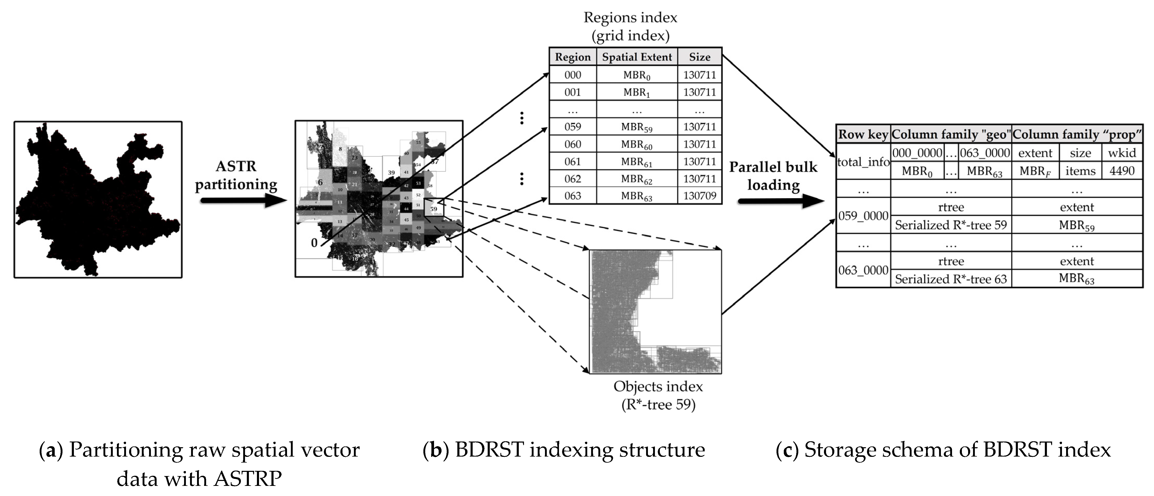
As Figure 4b shows, the regions index is a single grid index, and it records pairs of region identifier p i d and the minimum rectangle MBR p i d that enclose all the objects of each region. The regions index is saved as a single row in the HBase table, whose row key is “total info”. It can filter regions by checking the spatial relationship between MBR p i d and the query geometry to avoid access to all regions in spatial-query processing. The objects’ indexes are the p R*-trees corresponding to p partitions. In each HBase region, there is an R*-tree index that indexes the local spatial objects and is serialized and stored as the first row in the local region. R*-trees are loaded into memory in parallel only if their regions are qualified by the regions index to avoid redundant accesses to regions.

3.5. Storage Schema of BDRST Index on HBase

A rational storage schema for the BDRST index and SVD on HBase is the basis for efficient spatial-query processing. We summarized the rules of thumb for the table schema [57] and the SVD storage schema [7,31,64] on HBase (Table 1).
In our spatial storage schema, all the objects are stored in a tall, narrow table to downsize rows and columns. The table has two column families. A column family, named geo, is for geometries or indexes. And the column family, named prop, is for attribute data or metadata. Each row only stores one object, which is either an index or a spatial object.
In the HBase table, rows are alphabetically sorted by the ASCII codes of their row keys. A HBase table can be split by the user-defined splits schema of certain row keys. To generate regions corresponding with pre-balanced partitions by ASTRP, the row keys are mostly in the form of “partid_code” where partid is the partition identifier and code is the spatial encoding. The only one exception is the row storing the regions index since its row key is the aforementioned “total_info”. To construct fixed-length keys, the partid must be left padded with zeros to the defined length l e n p r e (Equation (1)). For example, if an SVD has 99 partitions, the l e n p r e is 2. If p is 100, the l e n p r e is 3.
The length of code depends on the max depth of the R*-trees in the BDRST index since it encodes spatial objects with their routing paths in the R*-tree (Figure 5). An R*-tree clusters near spatial objects to a node, hence objects in the same node tend to be closer to each other. Based on that, we descend the R*-tree and retrieve the identifiers from every node of each spatial object and concatenate these qualifiers as code. All the R*-trees R i * in the BDRST index have the same depth due to the ASTRP process. In an R*-tree, the indexed entries are children of leaf nodes, so we set the length l e n s u f of the code part to R i * . d e p t h + 1 (Equation (1)). To illustrate, the code of geometry nine in Figure 5 is “021”.
{ l e n p r e = t o S t r i n g ( p ) . l e n g t h ,   l e n s u f = R i * . d e p t h + 1 .                    
According to the content, we define three basic types of rows:
Definition 1.
A global metadata row (GMR) is a special row as its key is “total_info”. GMR stores the global grid index and the global metadata of the whole data set. The column family “geo” contains p columns that contain the partids and M B R p a r t i d of each region.
Definition 2.
A local metadata row (LMR) is a row whose key is the start key of each region. Each LMR stores a serialized bytes array of R*-tree R i * and the M B R p a r t i d of each region. In particular, the code part of an LMR key is a string of l e n s u f zeros.
Definition 3.
A data row (DTR) is a row that stores a spatial object. In DTR, a spatial geometry is serialized into EsriShape bytes, and the attributes are saved as JSON strings.
Table 2 shows an instance of the proposed table schema when l e n p r e is 2 and the l e n s u f   is 4.

3.6. Server-Side Parallel Spatial-Query Processing on HBase

3.6.1. Processing Phases

According to the general processing phases in spatial query-based applications, the elapsed time model for spatial queries in parallel is given as:
T = T 0 + max 0 i < p ( l i + d i + g i + τ i ) + T 1 .
The total execution time is T ; T 0 is the preparation time for the query job, including initialization and submission; p denotes the number of parallel tasks; l i , d i , and g i represent the time costs for the index loading, querying, and geometry filtering phases, respectively; τ i is the time cost of local post-processing (e.g., counting and area summing). According to the wood barrel theory, the overall elapsed time for this parallel processing depends on the longest one of the parallel tasks. Finally, T 1 is the time cost for global post-processing, such as shuffle or aggregations.

3.6.2. Spatial-Query Processing Based on HBase Endpoint

We define and implement three Endpoint services based on HBase endpoint interfaces for server-side spatial-query processing, including rangeQryService, nearQryService, and applicationService. Their processing modes are similar.
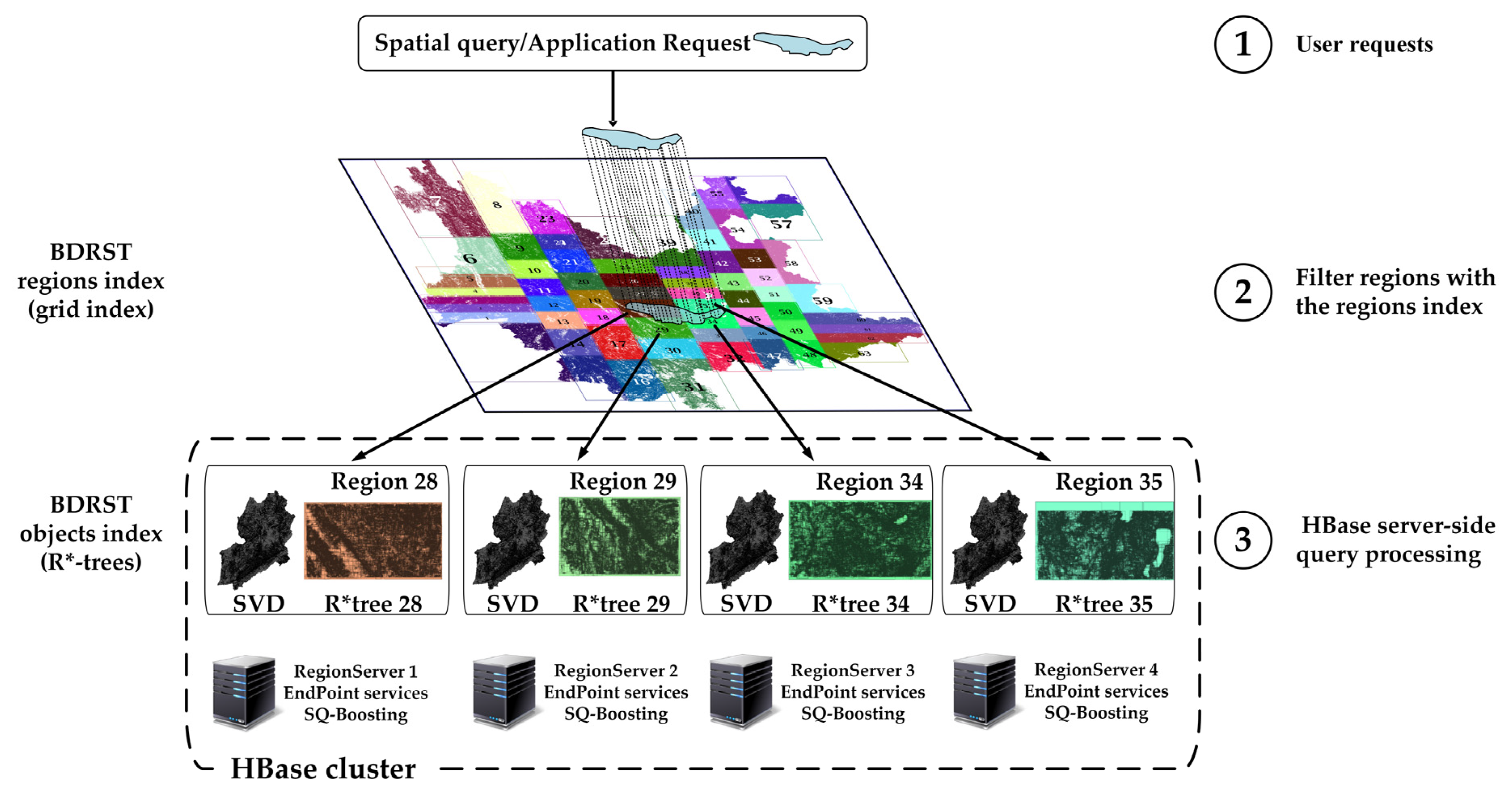
As shown in Figure 6, the processing framework accepts spatial-query requests and query-based application requests. The regions index is loaded on the client to pick out qualified regions. In each qualified HBase region, the objects index—a native R*-tree—is loaded by server-side endpoint services. The endpoints also can retrieve spatial objects in the current region with HBase functions, such as Base Get and Scan. Therefore, the processing framework can also handle a geometry filter and applications involving stored spatial vector data.
We also develop an SQ-Boosting mechanism with multithread processing to further accelerate the geometry filter and complex processing. An HBase endpoint task executes in a single thread by default. Hence, after R*-tree searching, the following computation-intensive processing tasks can be facilitated with multi-thread processing, i.e., to split R I into n subsets r I if R I exceeds the capacity threshold of single-thread processing and run n threads to process spatial objects addressed in r I (lines from 11 to 20 in Algorithm 1). We determine the n by:
n = R I . s i z e / t h r e s h o l d ,
and the max number of threads is estimated with the Venkat Subramaniam’s formula:
t h r e a d s = c o r e s / ( 1 k ) ,
where c o r e s is the number of available cores and k is the blocking coefficient, whose values are zero and one for CPU-intensive and IO-intensive tasks, respectively [66]. We set k to 0.2 since the spatial-query processing are more CPU-intensive. Algorithm 1 shows the SSCP-based processing phases of a spatial query.
Algorithm 1 SSCP-based spatial query processing.
Input: input geometry q , spatial predicate r , limit c
Output: query result R I or R G
/ * Step 1: Filter regions with the regions index.
Get the GMR gmr from the HBase table;
Foreach MBR p a r t i d in gmr do
    if MBR p a r t i d matches spatial predicate r with q
        Add partid to qualified region list regionlist;
Client launches a batch call that broadcasts q , r , c to the endpoint services on the regions addressed in regionlist;
/ * Step 2: Filter objects with the objects index in parallel
Foreach region in regionlist concurrently do
    Get byte array rtreebytes of the local R*-tree from the LMR;
    Deserialize rtreebytes and create an R*-tree instance R p a r t i d * ;
    Query R p a r t i d * with q , r , c and get query result R I ;
    if requires geometry filter then 
        if  R I .size > threshold then
            Split R I into n subsets according to the SQ-boosting configuration;
            foreach subset r I in n subsets do
                Start a new thread to perform the function geoFilter(partid, r I , q , r , c )
                Append the geoFilter result into the result set R G ;
        else
            Perform geoFilter(partid, R I , q , r , c ) and append the result into R G .
    else
          Append spatial objects mapped in R I to R G ;
    return query result R G to the client;
function geoFilter(partid, R I , q , r , c )
            for object identifier code in R I do
        Get geometry geo from the DTR by row key “partid_code”.
        if geo matches spatial predicate r with q then
            Append raw spatial vector data to local result set r G ;
    return  r G ;
In Step 1, the client queries the regions index (line 1) and finds the qualified regions (lines 2 to 4) whose MBR matches the spatial predicate r . Then, the client launches batch calls to broadcast query requests to the endpoint services on qualified regions (line 5).
In Step 2, the server-side endpoint services on qualified regions are triggered in parallel. Each service obtains the bytes of the serialized R*-tree (line 7), and deserializes and creates an R*-tree instance R p a r t i d * (line 8). Then the service performs R*-tree searching (line 9). If the current query requires a geometry filter, objects addressed in R I are retrieved and further filtered with a geoFilter function (lines 21 to 26). If R I is too large, the endpoint service also employs the SQ-Boosting for faster processing (line 11 to 15). The fine-filtered spatial objects are returned to the client. For spatial queries that do not require a geometry filter, the SVD addressed in R I will be retrieved and returned to the client.

3.6.3. Processing of Query-Based Applications

Processing query-based applications only requires the replacement of the geoFilter function with application functions. We only need to enhance the functions over endpoint interfaces. Algorithm 2 is an instance function of the LUCR application processing. It retrieves the raw spatial objects geo mapped in IRQ results (line 1 to 2) and calculates the intersection between geo and q (line 3 to 4). Finally, it summarizes the area data of the intersection and returns the results (line 5 to 8).
Algorithm 2 Land-use compliance review processing function.
Input: partition identifier partid, index query result set R I , input geometry q
Output: land-use compliance review result R A
foreach objects code code in R I do
    Get geometry geo and raw SVD f from the DTR by row key “partid_code
    if geo intersects with q then
        Calculate the intersection resgeo between geo and q
        Calculate the planar and geodesic area of resgeo
        Put areas and other statistical data into f i and format f i
        Append f i into result set R A
   return  R A to the client.

4. Experimental Evaluation

In this section, we evaluate the performance of our method with a series of experiments.

4.1. Measurement Metrics

We construct metrics of the distributed spatial index quality (DIQ) and query performance for evaluation. The query and application performance are estimated by their execution time. The DIQ affects the number of regions that need to be accessed and the redundant accesses in spatial-query processing. Previous DIQ metrics include DIQE, DIQO, and DIQD [7,24]; we propose a new metric DIQJ to measure the distance-preserving properties [22] of the distributed spatial indexes. Moreover, it is widely believed that building R*-trees is a time-consuming job, and index-building time is also collected for comparison.
DIQE (DIQ-Evenness) is the standard deviation of the capacity of generated R*trees in each partition. The smaller the DIQE is, the more balanced the distributed spatial indices are.
DIQO (DIQ-Overlap) is the overlap area among the MBRs of regions. Since distributed spatial indices build over regions, the smaller the DIQO is, the fewer the R*trees loaded. In the ideal case, DIQO is 0, which means that there is no overlap among regions as well as R*trees. DIQO can be formulated as:
DIQO = i = 0 p 1 j = i + 1 p M B R i   M B R j / M B R F .
DIQD (DIQ-Dead space) is the ratio between the total area occupied by MBRs of all regions and the area of MBR F . It can be formulated as:
DIQD = i = 0 p 1 M B R i / M B R F .  
DIQJ (DIQ-Jump) is the ratio between the area of the MBR that just contains M B R i and M B R i + 1 and the area of their union. The small DIQJ means that two partitions with continuous ids are spatially close to each other. DIQJ can be expressed as follows:
DIQJ = i = 0 p 2 M B R i   M B R i + 1 / M B R i . Union ( M B R i + 1 ) .

4.2. Experimental Setup

The experiments are conducted on a Cloudera’s Distribution Including Apache Hadoop (CDH) cluster. The HBase version is 5.13.3-1.2.0. The HBase cluster contains 3 HMasters and 4 Region Servers, each of them has 24 cores and 80 GB RAM, where Geomesa (version 1.3.5) is deployed. ArcSDE 10.6 is configured on an Oracle 12C database with 128 GB RAM and 20 threads. The nodes in CDH are interconnected with a 10-gigabit switch. All spatial-query requests are sent from the HBase master node to reduce the influence of communication costs on performance. We configure the memory of tasks in all MapReduce or Spark jobs to 4 GB.
SpatialHadoop is a full-fledged MapReduce framework with native support for spatial data on a Hadoop distributed file system [67]. It provides various spatial indices and spatial partitioning methods [7]. We choose SpatialHadoop to compare the DIQ and query efficiency of distributed spatial indices from SpatialHadoop with our BDRST index.
Geomesa is an open-source suite of tools that enables large-scale geospatial queries and analytics over column-family NoSQL databases [19]. Geomesa adopts an XZ-ordering-based index called XZ2. It also employs SSCP for efficient spatial-query processing. We use it to compare the performance and scalability with our method.
We use real-world datasets in Yunnan Province, China, as the experimental datasets. The datasets vary in the number of items, vertices, and data size to estimate the scalability of all methods. The details of the experimental data sets are shown in Table 3.

4.3. Experimental Results

4.3.1. Distributed Spatial Index Quality Evaluation

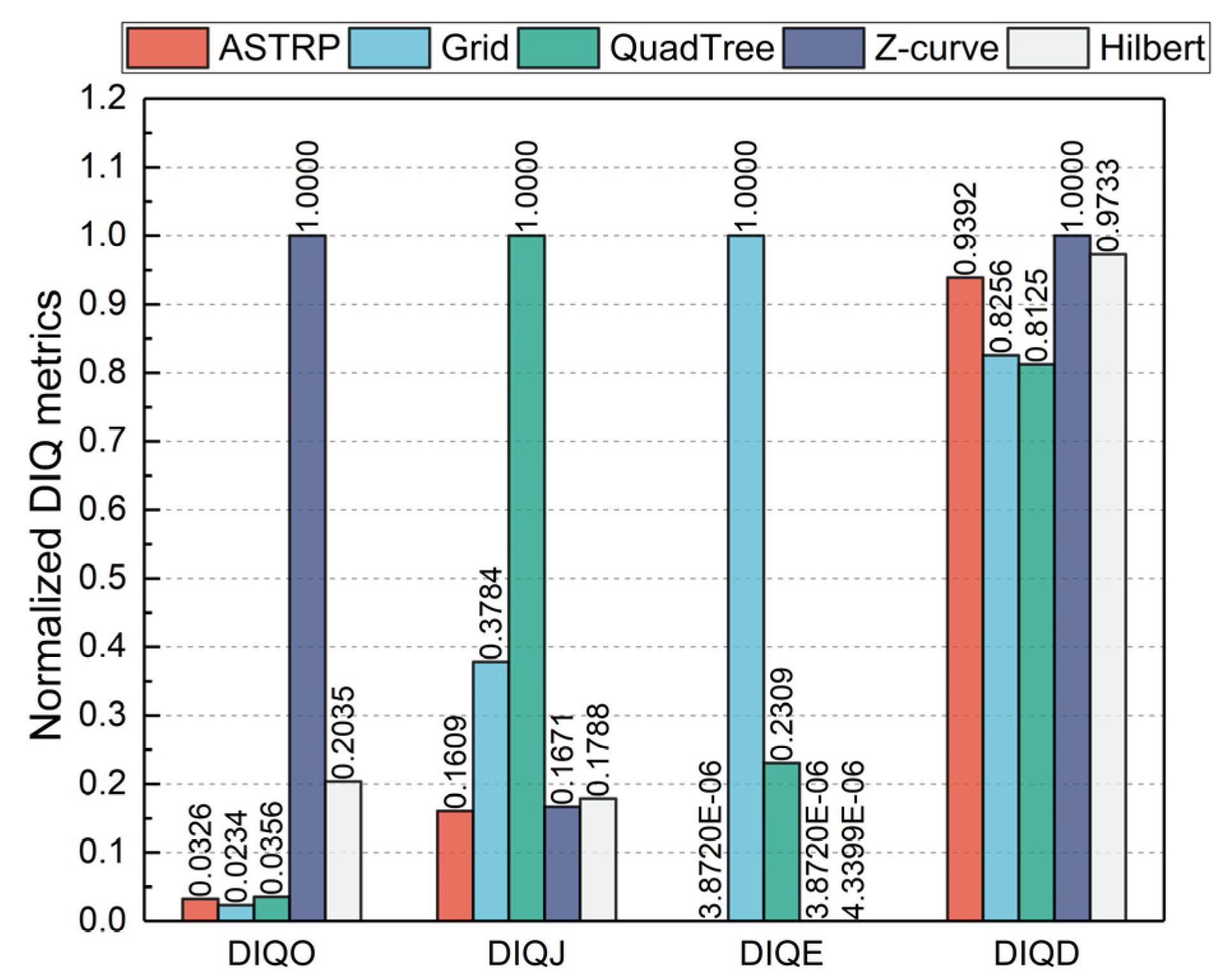
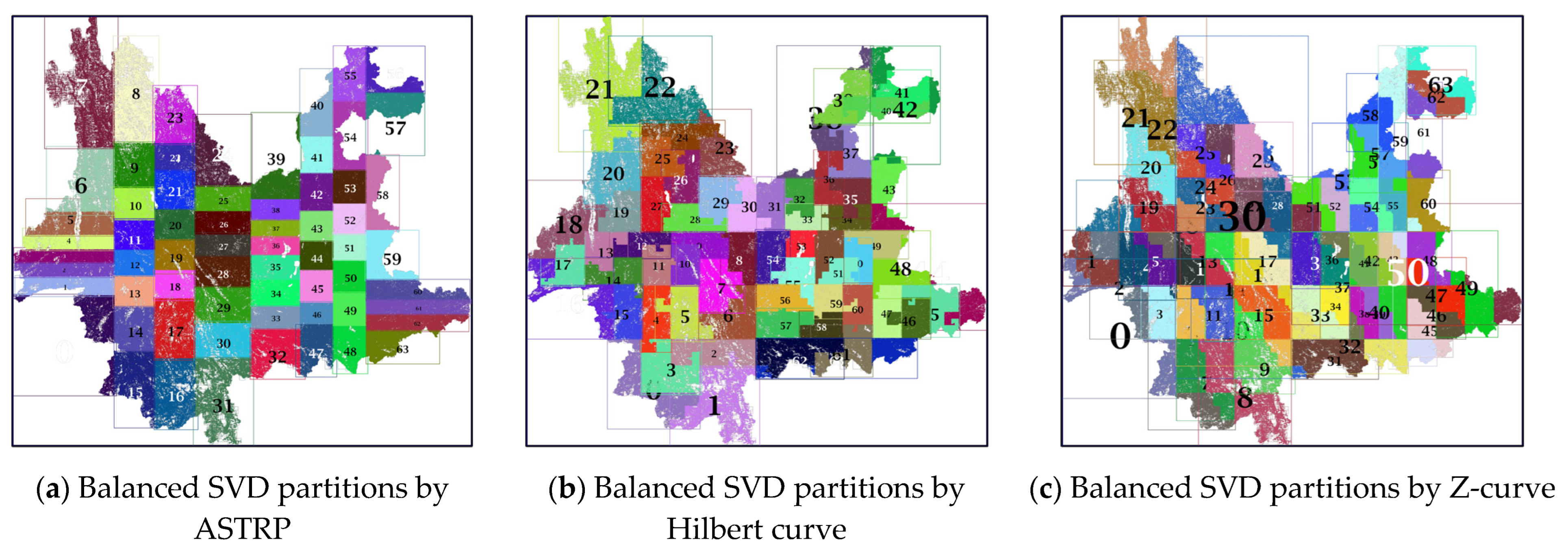
Figure 7 shows the normalized DIQ metrics of distributed spatial indexes built on D 4 . To intuitively show the DIQ, we also developed an Apache Spark job to render the partitioned SVD in Figure 8.
The grid and quad-tree show lower DIQO and DIQD, as they allocate objects in a regular split space; however, their DIQE and DIQJ are high because the distribution of the spatial objects is ignored. The raw DIQE values of ASTRP, Grid, Quadtree, Z-curve, and Hilbert are 0.4939, 127545, 29448, 0.4939, and 0.5535, respectively. The Z-curve and Hilbert curve show good evenness among partitions, as they partition SVD by equally slicing the one-dimensional orderings, but their DIQO and DIQD values are higher than others because the slicing may occur within the cells instead of borders. Spatial ranges of partitions encroach with each other as Figure 8 shows. Also note that a bigger overlap may reduce the jump between partitions, as distributed spatial indexes with higher DIQO value generally have lower DIQJ value.
The ASTRP strategy shows the lowest DIQE and DIQJ values, and the second-lowest DIQO value. The DIQD value of the ASTRP was the third of the five balancing strategies. Building the BDRST index on partitions split by ASTRP ensures evenness in R*-tree capacity and the best distance-preserving properties in HBase storage. The small DIQO value means fewer regions are accessed in spatial-query processing. As for DIQD, ASTRP is still better than the Hilbert curve and Z-curve methods. Note that the dead spaces in each region can be further pruned by the R*-trees.

4.3.2. Index-Building Efficiency

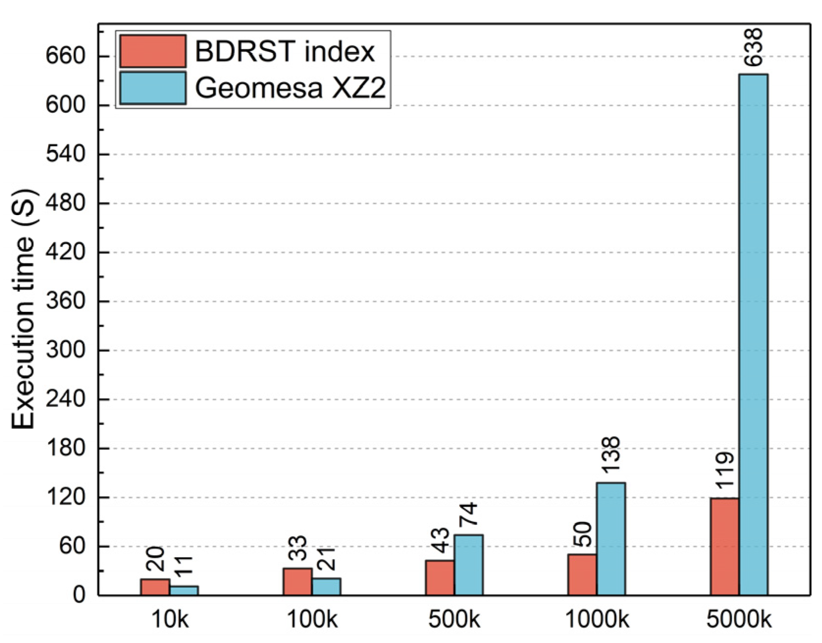
We randomly took 10,000 to 5,000,000 objects from D 4 and recorded the average execution time for five-round index-building executions. Geomesa builds the XZ2 index with a MapReduce ingest job, and our BDRST index was built with a Spark job. Both of them run in distributed mode.
According to Figure 9, Geomesa is more efficient in index building when the number of objects is less than 500,000. The level of XZ2 index is relatively small and the inserting cost is low. The BDRST index are faster in building time as the number of objects reaches 500,000 and are less sensitive to the growing data volume. Building the BDRST index for five million polygons only takes 119 s, whereas Geomesa needs over 10 minutes. The average building time of the BDRST index was 30.05% that of the Geomesa XZ2.
The insensitivity to data size of the BDRST index in building time comes from the ASTRP strategy that balances the SVD to equal-item partitions. Building an R*-tree on such a partition is to insert a fixed number of objects regardless of the size of the entire SVD. Also note that ASTRP reduces the data skewness in building tasks to improve the whole building performance, which is also important for a distributed job.

4.3.3. Intersection-Range-Queries Performance

We perform IRQs on Geomesa XZ2 and our BDRST index with varying query ranges listed in Table 4 on dataset D 4 . The plain IRQ is to query the spatial index with the MBRs and search spatial objects whose MBRs intersect with the query MBR. The IRQ with geometry filters queries the spatial index and checks the intersection between raw spatial geometries. All query requests are sent from the HBase master node.
Figure 10 depicts the average execution times for IRQs with the BDRST index and Geomesa XZ2. Geomesa shows relatively good performance for small and middle-range index queries. For both types of IRQs, when the query range is smaller than M 3 , Geomesa XZ2 can respond within 0.56 s. However, the rapidly increasing execution time for IRQs as the query range reaches and exceeds M 3 shows that Geomesa is not the best choice to perform large-scale IRQs. The disk-based Geomesa XZ2 index incurs large range table scans for the IRQs with a big query range, which leads to the slow spatial-query processing with heavy I/O operations. On the flipside, the execution time of Geomesa XZ2 index between plain IRQs and IRQs with geometry filters are very close since they both need to access actual rows due to the disk-based indexing scheme. As proof, performing an IRQ with geometry filters on M 6 yields an additional 1.4534 s; compared to performing a plain IRQ, the increase is only 7.9% of the execution time for the plain IRQ.
The BDRST index shows remarkable superiority in efficiency for both types of IRQs with all varying query ranges. For plain IRQs, the longest execution time is 0.6876 s on M 6 , and the execution time is less than 0.151 s before M 5 . The increases on M 5 and M 6 suggest that such large-scale IRQ requires big parallelism and reaches the performance limits of the current environmental HBase cluster. For IRQs with geometry filters, the execution time is less than 0.71 s before M 6 , which means that the BDRST index can provide a sub-second response for large-scale spatial range queries involving millions of results. The execution time on M 6 for IRQ with a geometry filter is 1.4419 s, which is much smaller than that of the Geomesa XZ2.
The numerical increases in execution time between the IRQs with geometry filters and plain IRQs of the BDRST index are smaller than that of Geomesa XZ2. As proof, the average additional time cost of the BDRST index is 0.39 s, while in Geomesa, this value is 0.68 s. Nevertheless, the proportional increases in the execution time for geometry filters in the BDRST index is bigger than Geomesa XZ2. According to Figure 10, we can calculate the proportion of the additional time for the IRQs with a geometry query by comparing with plain IRQs. This value is 44.96% on M 5 and 109.7% on M 6 . This suggests that the memory-based BDRST can directly process plain IRQs without accessing DTRs in HBase, while the IRQs with geometry filters demand accesses to DTRs to check the topological relations between intact geometries and the query geometry. Consequently, the I/O costs increase the processing time.
In general, the average execution time of plain IRQs with the BDRST index is 4.06% of the time with Geomesa XZ2, and the average execution time for IRQs with geometry filters with the BDRST index is 9.26% of the time with Geomesa XZ2.

4.3.4. kNN-Queries Performance

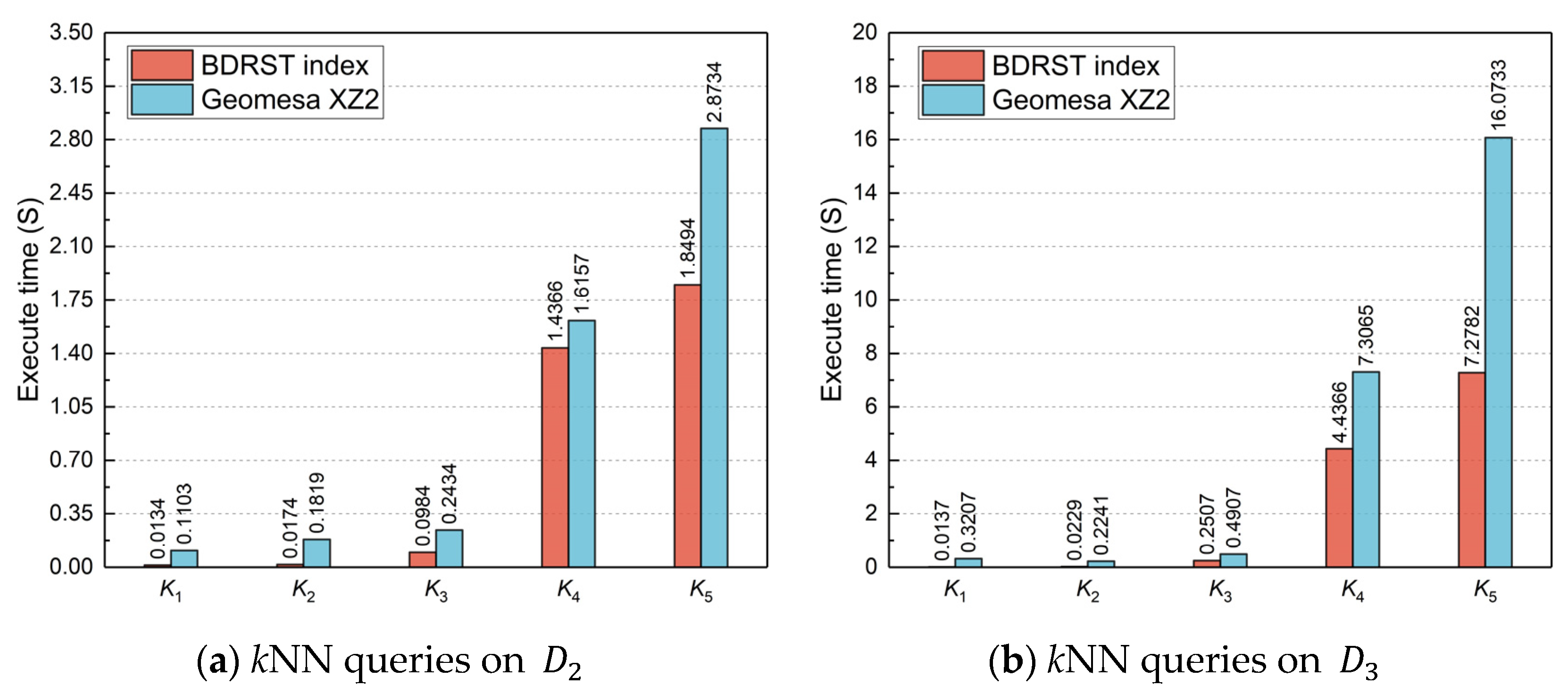
We perform kNN queries on the BDRST index and Geomesa on datasets D 2 and D 3 in different scales. As Table 5 shows, we randomly choose a center point with varying values of k and max searching radius to avoid filtering the whole dataset and compare the performance.
Figure 11 shows the average execution time for kNN queries with the BDRST index and Geomesa XZ2. The kNN-query performance gap between the BDRST index and Geomesa XZ2 is much smaller than the IRQs, which suggests that the BDRST index is more efficient for spatial range queries with rectangular query geometries. However, it still shows considerably high performance and scalability. On average, the execution time with the BDRST index is 50.1% of the Geomesa XZ2 on K 5 . The average execution time of all kNN queries with the BDRST index is 67.87% of Geomesa’s on D 2 and 49.16% on the larger dataset D 3 , which shows the better scalability of the BDRST index.

4.3.5. Application Performance

We perform LUCR applications on the BDRST index, Geomesa XZ2, and Esri ArcSDE (multilevel grids). In the processing phases, the LUCR searches all objects that intersect with the input polygons, computes the intersections between them, joins the properties, and computes statistics about the intersections. Table 6 shows the input polygons with varying spatial ranges and number of vertices for the LUCR.
As Figure 12 shows, the BDRST index shows the best LUCR performance. The average execution time for all tests with the BDRST index is 10.68% and 72.64% of that with ArcSDE grid and Geomesa XZ2, respectively. The increases in the execution time are greater as the input polygon enlarges due to the more intensive computations in LUCR. The results verify the scalable performance in the BDRST index and server-side parallel processing framework, and the applicability in spatial-query-based applications.

5. Conclusions and Future Work

Designing an efficient spatial index for NoSQL databases is important for both sustainability research and Green IT. This paper presents a BDRST index based on server-side in-memory R*-trees for efficient spatial-query processing of massive spatial vector data on HBase. The BDRST index is created on SVD partitions that are split and balanced by our ASTRP strategy to control the memory and storage overhead of R*-trees. The BDRST index stores and distributes serialized R*-trees to HBase regions along with SVD in one single table for server-side real-time instantiation instead of flattening them as a new table for disk-based tree searching in previous solutions. We use HBase coprocessor interfaces to implement a parallel processing mechanism for server-side parallel loading of localized R*-trees in each region and custom processing to improve the spatial-query processing performance. Hence, the BDRST index follows an on-demand in-memory usage since the lightweight R*-trees are dynamically loaded into and wiped out from the HBase memory heap with the start and end of the spatial-query processing to utilize the memory resource, instead of persisting permanently. The BDRST index supports two typical spatial queries: intersection range queries and kNN queries and the applications based on these spatial queries.
Extensive experiments are conducted on a CDH HBase cluster with real-world land-use-related data sets. The experimental results show the superiority of the BDRST index when compared with current disk-based spatial indexes. According to the distributed spatial index quality evaluation, the BDRST index shows the best distance-preserving properties and evenness in capacity among R*-trees, small overlap between R*-trees, and moderate dead spaces. The experiments in index-building efficiency demonstrate the low cost for building the BDRST index on HBase, since it saves 519 s when compared with the Geomesa XZ2 index with five million polygons. The third experiment of intersection range queries verifies the capability of the BDRST index to handle spatial range queries with millions of results; it provides sub-second response for plain IRQs and only needs less than two seconds for IRQs with geometry filters. The fourth experiment analyzes the kNN-queries performance of the BDRST index and the impact of varying values of k. The result indicates that the BDRST index is more efficient and scalable for kNN-query processing when compared with Geomesa XZ2. In the last experiment, we evaluate the application performance of the BDRST index with a common application in natural resource management called LUCR, where our index achieves higher performance than Geomesa and ArcGIS. The BDRST index shows good applicability in spatial-query-based applications.
Our proposed method provides an applicable and efficient in-memory spatial index for faster spatial-query processing on HBase. It presents a time-efficient spatial-query processing method for spatial applications and sustainability research that involve massive georeferenced data indicators. It also follows the Green IT rules to enhance energy efficiency with the improvement of spatial indexes on HBase. In future work, we plan to quantify the energy consumption of our BDRST index and compare it with other solutions, and study the impact of potential factors on power consumption in spatial-query processing, such as spatial index types, query ranges, communication costs, etc. Another extension we intend to explore is to find a real-time visualization solution for massive spatial data on HBase, which may require a further improved index structure and novel SSCP-based solutions.

Author Contributions

L.S. proposed the idea of the BDRST index and designed and implemented the index and the spatial-query processing algorithms. B.J. provided key suggestions and help on conceptualization and experimental evaluation. L.S. performed experiments and analyzed the results data. L.S. wrote this paper and B.J. helped to improve the manuscript. All authors have read and agreed to the published version of the manuscript.

Funding

This research was funded by National Natural Science Foundation of China (NSFC), grant number 41661086.

Institutional Review Board Statement

Not applicable.

Informed Consent Statement

Not applicable.

Data Availability Statement

Not applicable.

Conflicts of Interest

The authors declare no conflict of interest.

References

  1. Bakker, K.; Ritts, M. Smart Earth: A meta-review and implications for environmental governance. Glob. Environ. Chang. 2018, 52, 201–211. [Google Scholar] [CrossRef]
  2. Wang, S.H.; Sun, Y.R.; Sun, Y.L.; Guan, Y.; Feng, Z.H.; Lu, H.; Cai, W.W.; Long, L. A Hybrid Framework for High-Performance Modeling of Three-Dimensional Pipe Networks. ISPRS Int. J. Geo-Inf. 2019, 8, 441. [Google Scholar] [CrossRef] [Green Version]
  3. Huang, K.J.; Wang, C.L.; Wang, S.H.; Liu, R.Y.; Chen, G.X.; Li, X.L. An Efficient, Platform-Independent Map Rendering Framework for Mobile Augmented Reality. ISPRS Int. J. Geo-Inf. 2021, 10, 593. [Google Scholar] [CrossRef]
  4. Heitzler, M.; Lam, J.C.; Hackl, J.; Adey, B.T.; Hurni, L. GPU-Accelerated Rendering Methods to Visually Analyze Large-Scale Disaster Simulation Data. J. Geovisual. Spat. Anal. 2017, 1, 3. [Google Scholar] [CrossRef]
  5. Zhou, Y.K.; Wang, S.H.; Guan, Y. An Efficient Parallel Algorithm for Polygons Overlay Analysis. Appl. Sci. 2019, 9, 4857. [Google Scholar] [CrossRef] [Green Version]
  6. Wang, S.H.; Zhong, Y.; Lu, H.; Wang, E.Q.; Yun, W.Y.; Cai, W.W. Geospatial Big Data Analytics Engine for Spark. In Proceedings of the 6th ACM SIGSPATIAL International Workshop on Analytics for Big Geospatial Data (BigSpatial), Redondo Beach, CA, USA, 7–10 November 2017; pp. 42–45. [Google Scholar]
  7. Eldawy, A.; Alarabi, L.; Mokbel, M.F. Spatial partitioning techniques in SpatialHadoop. Proc. VLDB Endow. 2015, 8, 1602–1605. [Google Scholar] [CrossRef] [Green Version]
  8. Yu, J.; Wu, J.; Sarwat, M. GeoSpark: A cluster computing framework for processing large-scale spatial data. In Proceedings of the 23rd SIGSPATIAL International Conference on Advances in Geographic Information Systems, Seattle, WA, USA, 3–6 November 2015; p. 70. [Google Scholar]
  9. Rueda-Ruiz, A.J.; Ogáyar-Anguita, C.J.; Segura-Sánchez, R.J.; Béjar-Martos, J.A.; Delgado-Garcia, J. SPSLiDAR: Towards a multi-purpose repository for large scale LiDAR datasets. Int. J. Geogr. Inf. Sci. 2022, 36, 992–1011. [Google Scholar] [CrossRef]
  10. Guo, D.; Onstein, E. State-of-the-art geospatial information processing in NoSQL databases. ISPRS Int. J. Geo-Inf. 2020, 9, 331. [Google Scholar] [CrossRef]
  11. Wang, S.H.; Zhong, Y.; Wang, E.Q. An integrated GIS platform architecture for spatiotemporal big data. Future Gener. Comput. Syst.-Int. J. Escience 2019, 94, 160–172. [Google Scholar] [CrossRef]
  12. Rys, M. Scalable SQL. Commun. ACM 2011, 54, 48–53. [Google Scholar] [CrossRef]
  13. Stonebraker, M. SQL databases v. NoSQL databases. Commun. ACM 2010, 53, 10–11. [Google Scholar] [CrossRef]
  14. Cattell, R. Scalable SQL and NoSQL data stores. Acm Sigmod. Rec. 2011, 39, 12–27. [Google Scholar] [CrossRef] [Green Version]
  15. Huang, W. What Were GIScience Scholars Interested in During the Past Decades? J. Geovisualization Spat. Anal. 2022, 6, 7. [Google Scholar] [CrossRef]
  16. Yue, P.; Tan, Z. 1.06-GIS Databases and NoSQL Databases. In Comprehensive Geographic Information Systems; Huang, B., Ed.; Elsevier: Oxford, UK, 2018; pp. 50–79. [Google Scholar]
  17. Chang, F.; Dean, J.; Ghemawat, S.; Hsieh, W.C.; Wallach, D.A.; Burrows, M.; Chandra, T.; Fikes, A.; Gruber, R.E. Bigtable: A distributed storage system for structured data. ACM Trans. Comput. Syst. 2008, 26, 1–26. [Google Scholar] [CrossRef]
  18. Li, R.; He, H.; Wang, R.; Huang, Y.; Liu, J.; Ruan, S.; He, T.; Bao, J.; Zheng, Y. Just: Jd urban spatio-temporal data engine. In Proceedings of the 2020 IEEE 36th International Conference on Data Engineering (ICDE), Dallas, TX, USA, 20–24 April 2020; pp. 1558–1569. [Google Scholar]
  19. Hughes, J.N.; Annex, A.; Eichelberger, C.N.; Fox, A.; Hulbert, A.; Ronquest, M. Geomesa: A distributed architecture for spatio-temporal fusion. In Proceedings of the Geospatial Informatics, Fusion, and Motion Video Analytics V, Baltimore, MD, USA, 20–21 April 2015; pp. 128–140. [Google Scholar]
  20. Samet, H. 2. Object-Based and Image-Based Image Representations. In Foundations of Multidimensional and Metric Data Structures; The Morgan Kaufmann Series in Computer Graphics and Geometric Modeling; Morgan Kaufmann Publishers Inc.: Burlington, MA, USA, 2005. [Google Scholar]
  21. Carniel, A.C.; Roumelis, G.; Ciferri, R.R.; Vassilakopoulos, M.; Corral, A.; Aguiar, C.D. Porting disk-based spatial index structures to flash-based solid state drives. Geoinformatica 2022, 26, 253–298. [Google Scholar] [CrossRef]
  22. BÖxhm, C.; Klump, G.; Kriegel, H.-P. Xz-ordering: A space-filling curve for objects with spatial extension. In Proceedings of the International Symposium on Spatial Databases, Hong Kong, China, 20–23 July 1999; pp. 75–90. [Google Scholar]
  23. Guttman, A. R-trees: A dynamic index structure for spatial searching. In Proceedings of the 1984 ACM SIGMOD International Conference on Management of Data, Boston MA, USA, 18–21 June 1984; pp. 47–57. [Google Scholar]
  24. Beckmann, N.; Kriegel, H.-P.; Schneider, R.; Seeger, B. The R*-tree: An efficient and robust access method for points and rectangles. In Proceedings of the 1990 ACM SIGMOD International Conference on Management of Data, Atlantic City, NJ, USA, 23–25 May 1990; pp. 322–331. [Google Scholar]
  25. Hadjieleftheriou, M.; Manolopoulos, Y.; Theodoridis, Y.; Tsotras, V.J. R-Trees: A Dynamic Index Structure for Spatial Searching. In Encyclopedia of GIS, Shekhar, S., Xiong, H., Zhou, X., Eds.; Springer International Publishing: Cham, Switzerland, 2015; pp. 1–13. [Google Scholar]
  26. Kothuri, R.K.V.; Ravada, S.; Abugov, D. Quadtree and R-tree indexes in oracle spatial: A comparison using GIS data. In Proceedings of the 2002 ACM SIGMOD International Conference on Management of Data, Madison, Wisconsin, USA, 3–6 June 2002; pp. 546–557. [Google Scholar]
  27. Xiang, L.G.; Huang, J.T.; Shao, X.T.; Wang, D.H. A MongoDB-Based Management of Planar Spatial Data with a Flattened R-Tree. ISPRS Int. J. Geo-Inf. 2016, 5, 119. [Google Scholar] [CrossRef] [Green Version]
  28. Jadallah, H.; Al Aghbari, Z. SwapQt: Cloud-based in-memory indexing of dynamic spatial data. Future Gener. Comput. Syst.-Int. J. Escience 2020, 106, 360–373. [Google Scholar] [CrossRef]
  29. Zhang, D.; Wang, Y.; Liu, Z.; Dai, S. Improving NoSQL storage schema based on Z-curve for spatial vector data. IEEE Access 2019, 7, 78817–78829. [Google Scholar] [CrossRef]
  30. Du, N.; Zhan, J.; Zhao, M.; Xiao, D.; Xie, Y. Spatio-temporal data index model of moving objects on fixed networks using hbase. In Proceedings of the 2015 IEEE International Conference on Computational Intelligence & Communication Technology, Ghaziabad, India, 13–14 February 2015; pp. 247–251. [Google Scholar]
  31. Wang, L.; Chen, B.; Liu, Y. Distributed storage and index of vector spatial data based on HBase. In Proceedings of the 2013 21st International Conference on Geoinformatics, Kaifeng, China, 20–22 June 2013; pp. 1–5. [Google Scholar]
  32. Simmonds, R.; Watson, P.; Halliday, J. Antares: A Scalable, Real-Time, Fault Tolerant Data Store for Spatial Analysis. In Proceedings of the 2015 IEEE World Congress on Services, New York City, NY, USA, 27 June–2 July 2015; pp. 105–112. [Google Scholar]
  33. Limkar, S.V.; Jha, R.K. A novel method for parallel indexing of real time geospatial big data generated by IoT devices. Future Gener. Comput. Syst. 2019, 97, 433–452. [Google Scholar] [CrossRef]
  34. Tang, M.; Yu, Y.; Malluhi, Q.M.; Ouzzani, M.; Aref, W.G. LocationSpark: A distributed in-memory data management system for big spatial data. Proc. VLDB Endow. 2016, 9, 1565–1568. [Google Scholar] [CrossRef]
  35. Keeble, B.R. The Brundtland report: ‘Our common future’. Med. War 1988, 4, 17–25. [Google Scholar] [CrossRef]
  36. Nimmagadda, S.L.; Reiners, T.; Burke, G. Big Data Guided Design Science Information System (DSIS) Development for Sustainability Management and Accounting. Procedia Comput. Sci. 2017, 112, 1871–1880. [Google Scholar] [CrossRef]
  37. da Fonseca, E.P.R.; Caldeira, E.; Ramos Filho, H.S.; e Oliveira, L.B.; Pereira, A.C.M.; Vilela, P.S. Agro 4.0: A data science-based information system for sustainable agroecosystem management. Simul. Model. Pract. Theory 2020, 102, 102068. [Google Scholar] [CrossRef]
  38. Balaprakash, P.; Dunn, J.B. Overview of data science and sustainability analysis. In Data Science Applied to Sustainability Analysis; Elsevier: Oxford, UK, 2021; pp. 1–14. [Google Scholar]
  39. Liu, Z.; Ye, C.; Chen, R.; Zhao, S.X. Where are the frontiers of sustainability research? An overview based on Web of Science Database in 2013–2019. Habitat Int. 2021, 116, 102419. [Google Scholar] [CrossRef]
  40. Tang, J.; Fang, Y.; Tian, Z.; Gong, Y.; Yuan, L. Ecosystem Services Research in Green Sustainable Science and Technology Field: Trends, Issues, and Future Directions. Sustainability 2022, 15, 658. [Google Scholar] [CrossRef]
  41. Sharma, S.; Anees, M.; Sharma, M.; Joshi, P. Longitudinal study of changes in ecosystem services in a city of lakes, Bhopal, India. Energy Ecol. Environ. 2021, 6, 408–424. [Google Scholar] [CrossRef]
  42. Văculișteanu, G.; Doru, S.C.; Necula, N.; Niculiță, M.; Mărgărint, M.C. One Century of Pasture Dynamics in a Hilly Area of Eastern Europe, as Revealed by the Land-Use Change Approach. Sustainability 2022, 15, 406. [Google Scholar] [CrossRef]
  43. Kimothi, S.; Thapliyal, A.; Singh, R.; Rashid, M.; Gehlot, A.; Akram, S.V.; Javed, A.R. Comprehensive Database Creation for Potential Fish Zones Using IoT and ML with Assimilation of Geospatial Techniques. Sustainability 2023, 15, 1062. [Google Scholar] [CrossRef]
  44. Delgado, A.; Issaoui, M.; Vieira, M.C.; Saraiva de Carvalho, I.; Fardet, A. Food composition databases: Does it matter to human health? Nutrients 2021, 13, 2816. [Google Scholar] [CrossRef]
  45. Mahajan, D.; Blakeney, C.; Zong, Z.J.S.C.I. Improving the energy efficiency of relational and NoSQL databases via query optimizations. Sustain. Comput. Inform. Syst. 2019, 22, 120–133. [Google Scholar] [CrossRef]
  46. Naseri, A.; Ahmadi, M.; PourKarimi, L. Reduction of energy consumption and delay of control packets in Software-Defined Networking. Sustain. Comput. Inform. Syst. 2021, 31, 100574. [Google Scholar] [CrossRef]
  47. Arora, S.; Bala, A. Pap: Power aware prediction based framework to reduce disk energy consumption. Clust. Comput. 2020, 23, 3157–3174. [Google Scholar] [CrossRef]
  48. Pankowski, T. Consistency and availability of Data in replicated NoSQL databases. In Proceedings of the 2015 International Conference on Evaluation of Novel Approaches to Software Engineering (ENASE), Barcelona, Spain, 29–30 April 2015; pp. 102–109. [Google Scholar]
  49. Stonebraker, M.; Cattell, R. 10 rules for scalable performance in ‘simple operation’ datastores. Commun. ACM 2011, 54, 72–80. [Google Scholar] [CrossRef] [Green Version]
  50. Li, L.H.; Liu, W.D.; Zhong, Z.Y.; Huang, C.Q. SP-Phoenix: A Massive Spatial Point Data Management System based on Phoenix. In Proceedings of the 20th IEEE International Conference on High Performance Computing and Communications (HPCC)/16th IEEE International Conference on Smart City (SmartCity)/4th IEEE International Conference on Data Science and Systems (DSS), Exeter, UK, 28–30 June 2018; pp. 1634–1641. [Google Scholar]
  51. Li, R.; He, H.; Wang, R.; Ruan, S.; Sui, Y.; Bao, J.; Zheng, Y. Trajmesa: A distributed nosql storage engine for big trajectory data. In Proceedings of the 2020 IEEE 36th International Conference on Data Engineering (ICDE), Dallas, TX, USA, 20–24 April 2020; pp. 2002–2005. [Google Scholar]
  52. Ma, T.; Xu, X.; Tang, M.; Jin, Y.; Shen, W. MHBase: A distributed real-time query scheme for meteorological data based on HBase. Future Internet 2016, 8, 6. [Google Scholar] [CrossRef]
  53. Xia, Y.; Chen, J.; Lu, X.; Wang, C.; Xu, C. Big traffic data processing framework for intelligent monitoring and recording systems. Neurocomputing 2016, 181, 139–146. [Google Scholar] [CrossRef]
  54. Robinson, J.T. The KDB-tree: A search structure for large multidimensional dynamic indexes. In Proceedings of the Proceedings of the 1981 ACM SIGMOD International Conference on Management of Data, Ann Arbor, MI, USA, 29 April–1 May 1981; pp. 10–18.
  55. Samet, H. The Quadtree and Related Hierarchical Data Structures. ACM Comput. Surv. 1984, 16, 187–260. [Google Scholar] [CrossRef] [Green Version]
  56. Zhao, K.; Jin, B.; Fan, H.; Yang, M. A data allocation strategy for geocomputation based on shape complexity in a cloud environment using parallel overlay analysis of polygons as an example. IEEE Access 2020, 8, 185981–185991. [Google Scholar] [CrossRef]
  57. Sharma, M.; Sharma, V.D.; Bundele, M.M. Performance analysis of RDBMS and no SQL databases: PostgreSQL, MongoDB and Neo4j. In Proceedings of the 2018 3rd International Conference and Workshops on Recent Advances and Innovations in Engineering (ICRAIE), Jaipur, India, 22–25 November 2018; pp. 1–5. [Google Scholar]
  58. Zheng, K.; Gu, D.P.; Fang, F.L.; Zhang, M.; Zheng, K.; Li, Q. Data storage optimization strategy in distributed column-oriented database by considering spatial adjacency. Clust. Comput.-J. Netw. Softw. Tools Appl. 2017, 20, 2833–2844. [Google Scholar] [CrossRef]
  59. Nishimura, S.; Das, S.; Agrawal, D.; El Abbadi, A.J.D. MD-HBase: Design and implementation of an elastic data infrastructure for cloud-scale location services. Distrib. Parallel Databases 2013, 31, 289–319. [Google Scholar] [CrossRef]
  60. Faloutsos, C.; Roseman, S. Fractals for secondary key retrieval. In Proceedings of the 8th ACM PODS, Philadelphia, PA, USA, 29–31 March 1989. [Google Scholar]
  61. Li, S.; Zhong, E.; Wang, S. An Algorithm for Hilbert Ordering Code Based on State-Transition Matrix. J. Geo-Inf. Sci. 2014, 16, 846–851. [Google Scholar] [CrossRef]
  62. Ma, Y.; Zhang, Y.; Meng, X. St-hbase: A scalable data management system for massive geo-tagged objects. In Proceedings of the International Conference on Web-Age Information Management, Beidaihe, China, 14–16 June 2013; pp. 155–166. [Google Scholar]
  63. Yu, J.; Sarwat, M. Two birds, one stone: A fast, yet lightweight, indexing scheme for modern database systems. Proc. VLDB Endow. 2016, 10, 385–396. [Google Scholar] [CrossRef] [Green Version]
  64. Yu, J.; Zhang, Z.; Sarwat, M. Spatial data management in apache spark: The geospark perspective and beyond. GeoInformatica 2019, 23, 37–78. [Google Scholar] [CrossRef]
  65. Leutenegger, S.T.; Lopez, M.A.; Edgington, J. STR: A simple and efficient algorithm for R-tree packing. In Proceedings of the Proceedings 13th International Conference on Data Engineering, Birmingham, UK, 7–11 April 1997; pp. 497–506. [Google Scholar]
  66. Subramaniam, V. 2.4 Concurrency in Computationally Intensive Apps. In Programming Concurrency on the JVM; Pragmatic Bookshelf: Raleigh, NC, USA, 2011; pp. 1–280. [Google Scholar]
  67. Eldawy, A.; Mokbel, M.F. Spatialhadoop: A mapreduce framework for spatial data. In Proceedings of the 2015 IEEE 31st International Conference on Data Engineering, Seoul, Republic of Korea, 13–17 April 2015; pp. 1352–1363. [Google Scholar]
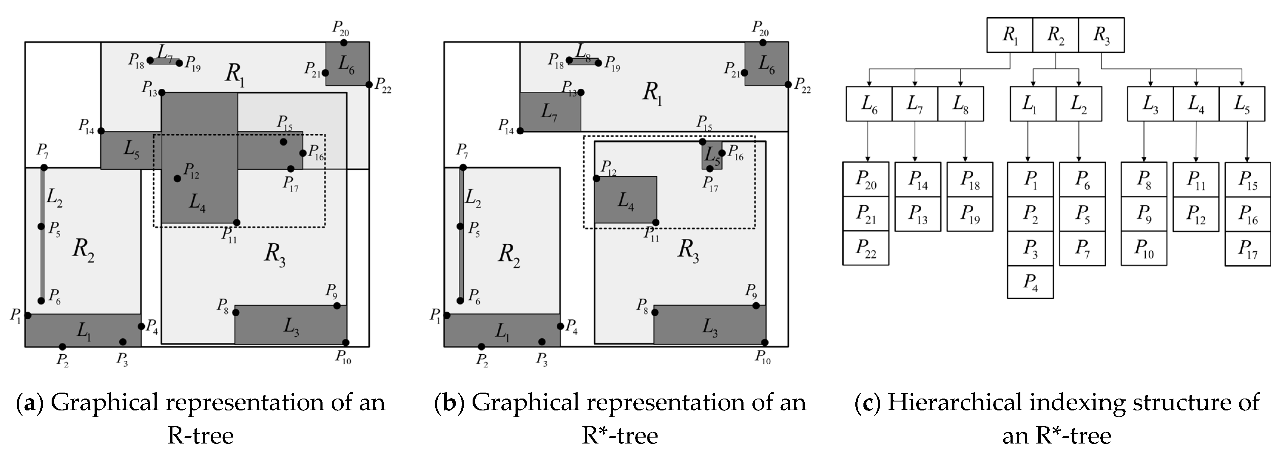
Figure 1. A comparison of an R-tree and an R*-tree. The graphical representation of an R-tree (a) and an R*-tree (b) and the hierarchical indexing structure of an R*-tree (c).
Sustainability 15 02442 g001
Figure 2. The architecture of spatial-query processing with BDRST index on HBase.
Sustainability 15 02442 g002
Figure 3. Comparison of spatial encoding strategies for partitions in STRP (a) and ASTRP (b).
Sustainability 15 02442 g003
Figure 4. The graphical representation of the BDRST index, including the SVD partitioning with ASTRP (a), structure (b), and storage schema (c) in HBase of the BDRST index.
Sustainability 15 02442 g004
Figure 5. An example of Spatial encoding for spatial objects with the routing paths in R*-tree.
Sustainability 15 02442 g005
Figure 6. Query processing framework with BDRST index and HBase Endpoints.
Sustainability 15 02442 g006
Figure 7. DIQ of distributed spatial indices generated by different balancing strategies on D 4 .
Sustainability 15 02442 g007
Figure 8. Renderings of the balanced partitions on D 4 by different balancing strategies.
Sustainability 15 02442 g008
Figure 9. Comparison of index building time between BDRST and Geomesa.
Sustainability 15 02442 g009
Figure 10. Comparison of IRQ performance of BDRST index and Geomesa XZ2 with varying query ranges on dataset D 4 .
Sustainability 15 02442 g010
Figure 11. Comparison of kNN-query performance between BDRST index and Geomesa XZ2 with varying values of k.
Sustainability 15 02442 g011
Figure 12. Comparison of LUCR performance of BDRST index, Geomesa XZ2, and ArcSDE grid with varying input polygons on different scales of datasets.
Sustainability 15 02442 g012
Table 1. Rules of thumb for the NoSQL storage schema of SVD and our measures.
Type of RulesRules of ThumbOur Measures
HBase table schema Minimum and short column familiesColumn families: “geo” and “prop”
Minimum rows and column sizesTall-narrow table for slim rows
Short and fixed-length row keysRow keys of two fix-length part
Even distributed rowsSpatial encoding based on R*-tree
Minimum number of versionsOne version for static SVD
Bytes-based storage in cellsSerialized BDRST index
SVD storage schema Data locality and index localityEach region stores a serialized R*-tree and an SVD partition
Minimum loading time of indicesBalanced, small, distributed R*-trees
High spatial index quality ASTRP strategy for BDRST index
Table 2. An instance of the storage schema for BDRST index and SVD on HBase.
Row KeyRow TypeColumn Family “geo”Column Family “prop”
total_infoGMR000_0000001_0000 p 1 _0000extentsizewkid
MBR 0 MBR 1 MBR p 1 MBR F 84532434490
000_0000LMRrtreeextent
byte array of serialized local R*-tree R 0 * MBR 0
000_0111DTRshapepropty
byte array of spatial geometry (EsriShape)byte array of properties (JSON)
000_0112DTRshapepropty
byte array of spatial geometry (EsriShape)byte array of properties (JSON)
p 1 _0000LMRrtreeextent
byte array of serialized local R*-tree R p 1 * MBR p 1
p 1 _0565DTRshapepropty
byte array of spatial geometry (EsriShape)byte array of properties (JSON)
Table 3. Details of the experimental datasets.
DatasetsContentsNumber of
Polygons (K)
Number of
Vertices (M)
Number of AttributesData Size (GB)
D 1 Ecological conservation redlines56.0661.57161.66
D 2 Permanent basic farmlands1950.19199.40246.55
D 3 Land patches of land-use planning data8132.81758.402123.81
D 4 Land patches of land-use data8365.48734.242324.75
Table 4. Details of the input MBRs for the index queries.
Query GeometrySpatial Extent (°)Number of Results
M 1 0.1 × 0.14796
M 2 0.5 × 0.532,520
M 3 1.0 × 1.0130,833
M 4 2.0 × 2.0666,153
M 5 3.0 × 3.01,789,596
M 6 4.0 × 4.04,293,851
Table 5. Details of the kNN queries.
Center PointkValues of kMax Searching Radius (°)
101.419725° E, 25.623202° N K 1 100.001
K 2 1000.01
K 3 10,0000.1
K 4 1,000,0001
K 5 2,000,0001.5
Table 6. Details of input polygons for land-use compliance review application.
Input
Polygons
Spatial
Extent (°)
Number of
Vertices
Return Items
D 1 D 2 D 3
G 1 0.01 × 0.0182513
G 2 0.03 × 0.0315010562
G 3 0.1 × 0.1302117627
G 4 0.3 × 0.380227271714899
G 5 1.0 × 1.015053426426115820
Disclaimer/Publisher’s Note: The statements, opinions and data contained in all publications are solely those of the individual author(s) and contributor(s) and not of MDPI and/or the editor(s). MDPI and/or the editor(s) disclaim responsibility for any injury to people or property resulting from any ideas, methods, instructions or products referred to in the content.