Use of Machine Learning Techniques in Soil Classification

Abstract

In the design of reliable structures, the soil classification process is the first step, which involves costly and time-consuming work including laboratory tests. Machine learning (ML), which has wide use in many scientific fields, can be utilized for facilitating soil classification. This study aims to provide a concrete example of the use of ML for soil classification. The dataset of the study comprises 805 soil samples based on the soil drillings of the new Gayrettepe–Istanbul Airport metro line construction. The dataset has both missing data and class imbalance. In the data preprocessing stage, first, data imputation techniques were applied to deal with the missing data. Two different imputation techniques were tested, and finally, the data were imputed with the KNN imputer. Later, a balance was achieved with the synthetic minority oversampling technique (SMOTE). After the preprocessing, a series of ML algorithms were tested with 10-fold cross-validation. Unlike the studies conducted in previous research, new gradient-boosting methods such as XGBoost, LightGBM, and CatBoost were tested, high classification accuracy rates of up to +90% were observed, and a significant improvement in the accuracy of prediction (when compared with previous research) was achieved.

1. Introduction

Soil classification is used to categorize soils with similar engineering properties based on a shared set of properties or characteristics. The behavior of soil is unlike other engineering materials such as steel or concrete due to its natural formation, geological history, and particulate nature [1]. The determination of soil properties and the explanation of soil behavior form the basis of geotechnical engineering. Soil classification usually depends on certain soil properties, such as grain-size distribution, liquid limit, and plasticity index [2]. Soil classification is important to classify soils with similar properties and to facilitate the dissociation of soils. With soil classification, soil is grouped according to similar properties that it shows when it is exposed to load [3]. Soil classification is a must-do before a foundation design. It is very important to define and classify the soil for the research and design stages of geotechnical engineering processes. Thus, a soil survey should be conducted to determine the soil properties.

The correct classification of soils is essential from an engineering point of view. Soil classification is performed based on an analysis of soil properties. One of these is sieve analysis, which determines soil particle size. Based on the sieve openings and the amount of material remaining on the sieve, soil classification is achieved. Plasticity is another relevant parameter that ought to be taken under consideration for the soil classification procedure [4].

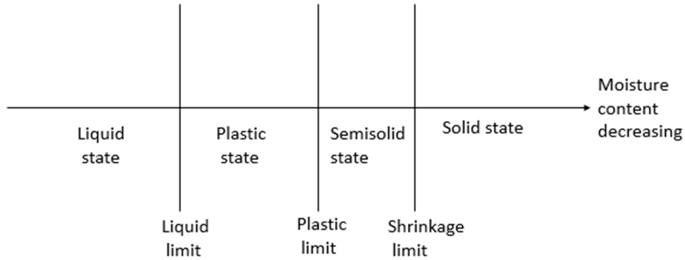
Atterberg [5] found a method to describe the state of fine-grained soil in terms of moisture content. The limits used to describe the state of the soil are the liquid limit (LL), plastic limit (PL), and shrinkage limit (SL). As shown in Figure 1, with drying, the soil sample changes to a semisolid state and a solid state [6].

The liquid limit (LL) and the plasticity index (PI) are important parameters in defining and classifying soil. The moisture content from a plastic to a liquid state is the liquid limit, and the moisture content at the point of transition from a semisolid to a plastic state is the plastic limit [7]. Casagrande [8] determined the liquid limit experimentally. The Casagrande cup and fall cone methods can be used to determine the liquid limit. The plastic limit test is simple and is performed by repeated rolling of an elliptic soil mass by hand on a ground glass plate [7]. The numerical difference between the liquid limit and the plastic limit is defined as the plasticity index. Soil classification can be performed by using the liquid limit and plasticity index values on the Casagrande plasticity card [7].

In mechanical analysis, the size range of particles in the soil is specified as a percentage of the total dry weight. Sieve analysis is one of the methods used to determine the particle size distribution of the soil [7]. In sieve analysis, the soil sample wobbles and shrinks as it passes through sieves with different aperture sizes. [9]. The sieving process is monitored by weighing the sieves at regular intervals [10]. US standard sieve numbers and the sizes of openings in mm are given in

Table 1. US standard sieve sizes [7].

Sieve No.	Opening (mm)	Sieve No.	Opening (mm)
4	4.75	35	0.500
5	4.00	40	0.425
6	3.35	50	0.355
7	2.80	60	0.250
8	2.36	70	0.212
10	2.00	80	0.180
12	1.70	100	0.150
14	1.40	120	0.125
16	1.18	140	0.106
18	1.00	170	0.090
20	0.85	200	0.075
25	0.710	270	0.053
30	0.600

.

A practical common language is generated in geotechnical engineering through soil classification. There are many soil classification systems available. The classification systems developed for fine-grained soils are the Unified Soil Classification System (USCS), the American Association of State Highway and Transportation Officials (AASHTO), and the Federal Aviation Agency system [11].

In the soil classification process, the operation starts in a well-equipped lab, a good interpretation of experimental findings can be only accomplished by an experienced geotechnical engineer leading a skilled team, and this process is costly [12]. Machine learning can be used to classify the ground classes obtained by various experimental studies without the need for experimental work.

Moreno-Maroto et al. [11] stated in their studies that when classifying soil, parameters other than grain size should be examined, such as plasticity. For that reason, the liquid limit and plasticity index were added, as well as sieve analysis, when classifying the soil in the coverage of that study.

Soil–structure interaction is an interdisciplinary issue that has been addressed since the end of the 19th century [13]. Evaluation of the soil–structure interaction while monitoring the building’s response is important, as the material properties of the underlying soil can change the ground motion at the soil–foundation interface [14]. Therefore, it is necessary to know the soil and its properties for all structures.

In recent years, the architecture, engineering, and construction (AEC) industry has been benefiting much from artificial intelligence and machine learning. Several studies on machine learning in civil engineering exist in the recent literature, including a classification of failure modes [15,16], performance classifications and the prediction of reinforced masonry structures [17], a prediction of the optimum parameters of passive-tuned mass dampers [18,19], an estimation of the optimum design of structural systems [20], prediction models for optimum fiber-reinforced polymer beams [21,22], a prediction of the axial compression capacity of concrete-filled steel tubular columns [23], a prediction of the bearing strength of double shear bolted connections [24], and predictions of the shear stress and plastic viscosity of self-compacting concrete [25] and for the optimum design of cylindrical walls [26].

As in many engineering fields, the use of artificial intelligence (AI) has become widespread in geotechnical engineering. Recently, AI approaches such as machine learning (ML), artificial neural networks (ANN), and deep learning (DL) have become popular among geotechnical engineers. For instance, Isik and Ozden [27] examined the estimation of the compaction parameters of coarse and fine-grained soils through ANN models using different input datasets. They found that the generalization capability and prediction accuracy of ANN models could be further enhanced by sub-clustered data division techniques. Momeni et al. [28] carried out a study to estimate the bearing capacity of piles with a genetic algorithm (GA) optimization technique. The inputs of the GA-based ANN model are the pile geometric properties, the pile set, and the hammer weight and drop height, and the output was the pile’s ultimate bearing capacity. They found it advantageous to apply GA-based ANN models as a highly reliable, efficient, and practical tool for estimating pile-bearing capacity. Gambill et al. [29] effectively used the random forest model for predicting USCS soil classification type from soil variables. They found that predictions from RF were significantly better than previous crosswalk methods. Pham et al. [30] used and compared four machine-learning methods to predict the shear strength of soft soil. They concluded that a parsimonious network based on a fuzzy inference system (PANFIS) is a promising technique for predicting the strength of soft soils. Díaz et al. [31] presented neural networks to improve the determination of the influence factor (I_a), which considers the effect of a finite elastic half-space limited by the inclined bedrock under a foundation. The results obtained through the application of artificial neural networks (ANNs) demonstrated a notable enhancement in the predicted values for the influence factor in comparison with those of existing analytical equations. Puri et al. [12] suggested that most AI models are reliable in the prediction of missing data. Zhang et al. [32] tried to find a pressure module with artificial intelligence methods; this is an important parameter, as it affects the compressive deformation of geotechnical systems such as foundations and is also difficult and costly to find. The authors suggested that by applying ML algorithms, a system can become intelligent in self-understanding the relationship between input and output. A comparison of the performance of empirical formulas and the proposed ML method for predicting foundation settlement indicated the rationality of the proposed ML model. Momeni et al. [33] used machine learning techniques to estimate pile-bearing capacity (PBC). They found that the Gaussian process regression (GPR)-based model is capable enough to predict the PBC and outperforms the GA-based ANN model. The results showed that the GPR can be utilized as a practical tool for pile-bearing capacity estimation. Nguyen et al. [34] examined the effect of data splitting on the performance of machine learning methods in a prediction of the shear strength of soil through training/test set validation. They used 70% of the dataset for training and 30% of the dataset for testing. The results of this study have shown an effective way to select the best ML model and appropriate dataset ratios to accurately estimate the soil shear strength that will assist in the design and engineering phases of construction projects. Martinelli and Gasser [35] applied machine learning models for predicting soil particle size fractions. They compared performance in estimating particle size fractions in their study. In the study, soil pH, cation exchange capacity, and elements extracted with Mehlich-3 of 8364 soil samples taken from different parts of Canada were used as covariates for the estimation of texture components. The researchers reported that multiple linear regression and neural network models had the weakest prediction performance, and the models with the best prediction performance were reported as RF, KNN, and XGBoost. Nguyen et al. [4] suggested a new classification method for determining soil classes based on support vector classification (SVC), multilayer perceptron (MLP), and random forest (RF) models. The results indicated that the performance of all three models was good, but the SVC model was the best in the accurate classification of soils. Tran [36] used a single machine learning algorithm to predict and investigate the permeability coefficient of soil. The author showed that SHapley Additive exPlanations (SHAP) and Partial Dependence Plot 1D (PDP 1D) performed with the best performance aided by a reliable ML model, GB (gradient boosting).

Based on the review of previous research, the main aim of this study was determined as exploring new ML methods/algorithms to automatically classify soil for minimizing the time and cost of the process. In this study, a new perspective is provided for soil classification by utilizing different algorithms/classifiers for supervised learning.

2. Materials and Methods

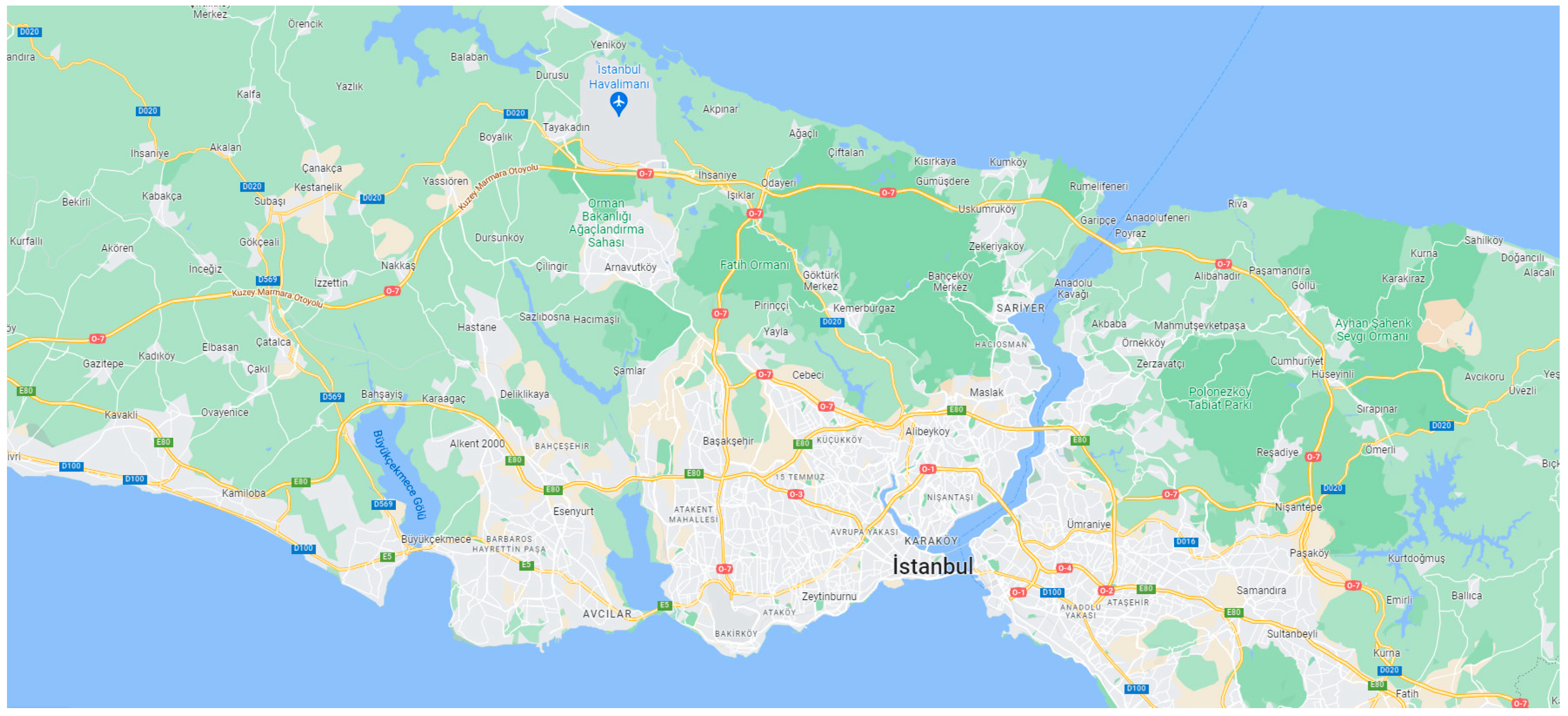
The soil classification dataset used in this study was developed by the authors and comprises records that were acquired from the soil drillings of the new Gayrettepe—Istanbul Airport metro line construction. The exploratory analysis model training and testing were carried out with the help of Python libraries, such as NumPy, Pandas, Matplotlib, and Scikit-learn. These libraries have been highly preferred in terms of accuracy and ease of use. NumPy is one of the most useful Python packages when it comes to creating applications requiring data science. It enables users to save and operate data as nd arrays (n-dimensional arrays) instead of the lists and dictionaries that are usually used for saving data in Python. One of the distinguishing features of nd arrays is their duration time in operations on data elements, which is much shorter when compared to the duration of operation time in Python lists [37]. Pandas has been used for reading the input and storing data with fast and efficient data frame objects [38]. MatPlotlib is an essential package for data scientists to demonstrate and analyze their findings in a visualized way. It is a plotting package that makes common plots easy and novel or complex visualizations possible [39]. Scikit-learn is the most commonly used machine learning library for the classification of tabular data [40]. In the study, the ML models were trained and tested by utilizing Python [41] as the language, Anaconda3 [42] as the environment, and Spyder 5.2.2 as the editor. Python was chosen as the coding language of this study, as it provides high accuracy and performance [43].

2.1. Exploratory Data Analysis

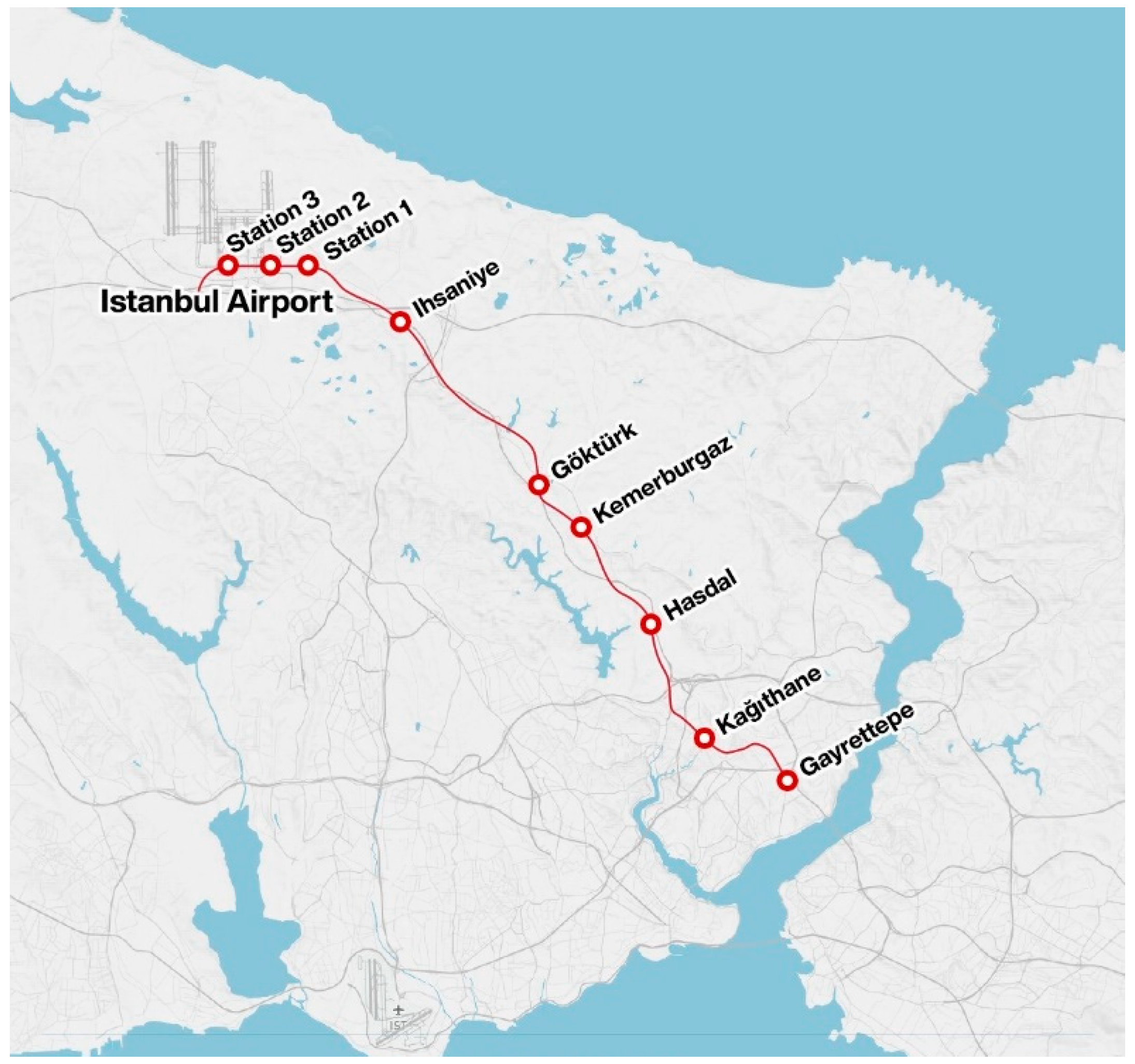
The dataset used in the study comprises 805 soil sample records that were acquired from the soil drillings of the new Gayrettepe–Istanbul Airport metro line construction (Figure 2 and Figure 3). The soil sample data were created using two methods. The first method was to obtain soil samples from a single borehole log but at different depths, and the second method included obtaining soil samples from different borehole logs. The data were collected to acquire the same number of records for each parameter of the dataset. Sometimes data were not available for a few parameters due to the variable state of the soil. In that case, data imputation was used to estimate unknown parameters. The soil classification was performed according to the Standard Test Method for Classification of Soils For Engineering Purposes (ASTM D 2487:1969 EQV) [44]. Five parameters, which are common soil properties used in classification, were selected as the dataset parameters. The apertures of sieve sizes were chosen as 4.75 mm and 0.075 mm, as these are the sieve sizes used when soil classification is performed according to ASTM D 2487:1969 EQV [44].

Based on this decision, the parameters (features) of the dataset were determined as: a retaining No. 4 sieve, a passing No. 200 sieve, the liquid limit (LL), the plastic limit (PL), and the plasticity index (PI). Based on these parameters, the data were classified into 5 classes: high-plasticity clay (CH), low-plasticity clay (CL), clayey sand (SC), high-plasticity silt (MH), and medium-plasticity clay (CI).

High-plasticity clay (CH) is a fine-grained soil, of which more than 50% of its particles are smaller than 75 μm, its liquid limit is bigger than 50, it is inorganic, and in the plasticity chart, the PI is on line A.

Low-plasticity clay (CL) is a fine-grained soil, of which more than 50% of its particles are smaller than 75 μm, its liquid limit is fewer than 35, it is inorganic, and in the plasticity chart, the PI is bigger than 4, and the PI is on line A.

Clayey sand (SC) is a coarse-grained soil, of which more than 50% of its particles are bigger than 75 μm, and its fine grains can be low-plasticity clay (CL), medium-plasticity clay (CI), or high-plasticity clay (CH).

High-plasticity silt (MH) is a fine-grained soil, of which more than 50% of its particles are smaller than 75 μm, its liquid limit is bigger than 50, it is inorganic, and in the plasticity chart, the PI is under line A.

Medium-plasticity clay (CI) is a fine-grained soil, of which more than 50% of its particles are smaller than 75 μm, its liquid limit is between 35 and 50, it is inorganic, and in the plasticity chart, the PI is on line A.

In the dataset, a retaining No. 4 sieve (for particles), a passing No. 200 sieve (for particles), the liquid limit, the plastic limit, and the plasticity index were the inputs/features, and the soil class was the output variable. The basic statistics of the features are provided in

Table 2. Basic statistics of features.

Features	Min	Max	Mean	Standard Deviation
Retaining No. 4 sieve	0	29.4	0.4365	2.4987
Passing No. 200 sieve	13.0	100	90.8599	12.9337
Liquid limit	23.1	90.0	53.4743	11.7505
Plastic limit	3.4	36.9	23.3158	29.6082
Plasticity index	7.3	62.0	30.4820	11.0532

.

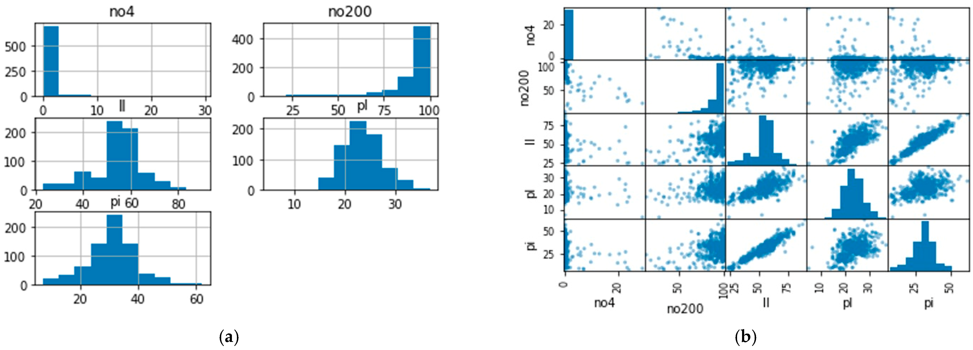
The histogram and scatter plots of the dataset are shown in Figure 4. In the figure, no4 stands for retaining No. 4 sieve, no200 stands for passing No. 200 sieve, ll is the liquid limit, pl is the plasticity limit, and pi denotes the plasticity index. Figure 4a shows that the liquid limit, the plastic limit, and the plasticity limit are (normal-like) distributed, No. 4 sieve values are close to 0 and highly positively skewed, and No.200 has a negatively skewed distribution. Figure 4b shows that the liquid limit and the plasticity index have a high positive correlation, the liquid limit and the plastic limit have a low positive correlation, and the No. 4 sieve and No. 200 sieve do not correlate with other parameters.

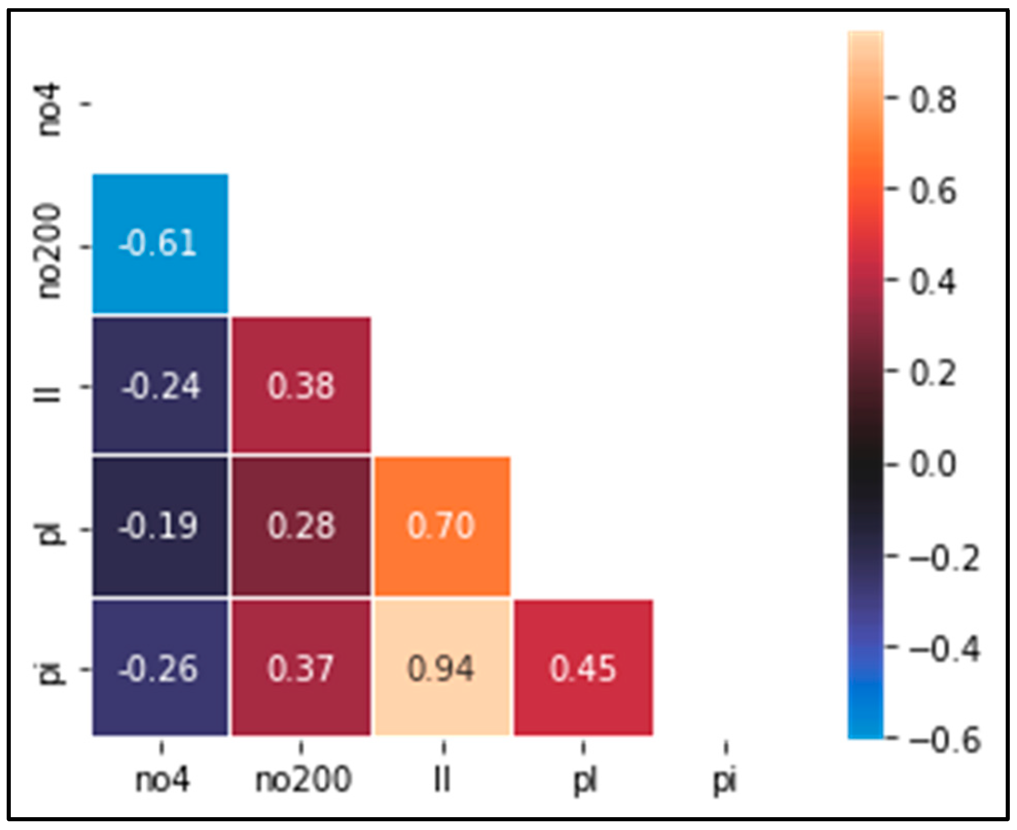
The correlation between the features is shown in Figure 5. According to the color scheme of the graph, cells of cream color indicate a high correlation, and the degree of correlation decreases gradually as the color nears black. The highest correlation is observed between the liquid limit and the plasticity index.

2.2. Data Preprocessing

The data preprocessing stage was focused on the transformation of data to achieve accurate prediction models. Based on the nature of the dataset, missing value imputation and data balancing techniques were used in this stage.

2.2.1. Missing Value Imputation

A missing value is a situation that can be encountered in real data. The need to collect data with missing values can be due to a malfunction of the test instrument, or missing values may also exist due to the respondents not answering some questions of a survey [46]. Missing values of features can reduce the performance of a ML algorithm. Therefore, prior to the model training, the missing value problem must be solved. Various methods are available to deal with this problem [47]. In our study, except for the feature “passing No. 200 sieve”, all features had missing data. The relative frequencies of missing data were 5.33%, 0.74%, 0.74%, and 6.32% for the retaining No. 4 sieve, the liquid limit, the plastic limit, and the plasticity index, respectively.

There were a total of 106 missing values in the dataset of 805×6 (RxC). In the imputation process, the missing (NaN) values were filled by utilizing a simple imputer with mean and the KNN imputer from the “Imputer” class of the “Scikit-learn” library. In the KNN imputer, the K-nearest neighbor approach is taken to complete missing values. In this approach, missing values in the attribute are filled with the average value of neighbors [48]. As explained in Section 3, the best-performing imputer was found as the KNN imputer and implemented for the imputation of the missing values in the dataset. The basic statistics for the dataset after data imputation with the KNN imputer are provided in

Table 3. Basic statistics of features after data imputation with KNN Imputer.

Features	Min	Max	Mean	Standard Deviation
Retaining No. 4 sieve	0	29.4	0.4836	2.6136
Passing No. 200 sieve	13.0	100	90.8523	12.9319
Liquid limit	23.1	90.0	53.4301	10.8526
Plastic limit	3.4	36.9	23.3168	4.1062
Plasticity index	7.3	62.0	30.0529	8.4294

.

As depicted in Figure 6, the highest correlation is still between the liquid limit and the plasticity index after the imputation process.

2.2.2. Dealing with Imbalanced Data

The imbalance in class distribution affects the success of classifiers [49]. In this study, since the soil formation can change even within one meter, an imbalance occurs naturally between the soil classes during the sampling, as some soil classes were observed too frequently, whereas some other soil classes were observed rarely in the process. The rate of observation of high-plasticity clay (CH) was 71%, low-plasticity clay (CL) was 21%, medium-plasticity clay (CI) was 3%, high-plasticity silt (MH) was 3%, and clayey sand (SC) was 2%. To tackle this imbalance, oversampling was deemed to be the appropriate method for balancing the data in terms of the dependent variable (i.e., soil class). The oversampling in the study was performed utilizing the synthetic minority oversampling technique (SMOTE) [49], which generates synthetic observations between the nearest neighbors of observations in the minority class [50]. The SMOTE method helped to generate a dataset with an equal distribution of the soil classes. Further details on the imbalance in class distributions and the application of the SMOTE process are provided in Section 3.

2.3. Classification with Machine Learning

Machine learning is a branch of artificial intelligence that is specifically focused on the automation of learning with tabular data, and its four sub-fields include supervised learning, unsupervised learning, semi-supervised learning, and reinforcement learning. In supervised learning, a model is developed with examples consisting of input and outputs. In this type of learning, the aim is to enable the machine to gain experience with certain (and provided) results to learn the path leading from the data to the results. In reinforcement learning, the machine learns by interacting with its environment. The technique is based on trial and error, where the model aims to win the most prizes until the target [51,52]. Unsupervised learning has no labeled output. Some features that the algorithm learns emerge from the data. The semi-supervised learning model is a combination of the supervised learning and unsupervised learning models [53]. The purpose is to improve learning performance by using abundant unlabeled data with limited labeled data [54].

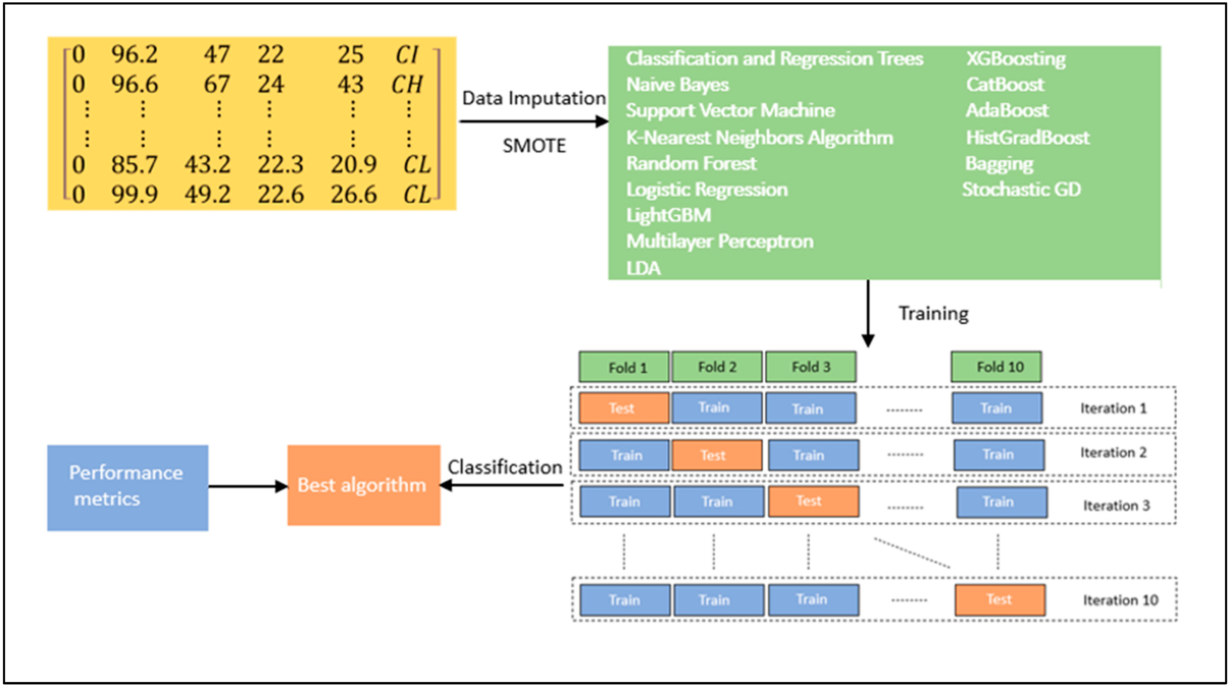
A general scheme of the supervised machine learning process is implemented in this study, as illustrated in Figure 7. The dataset used in this study has a multi-class categorical target variable with a label. Thus, classification algorithms/classifiers had to be implemented to formulate a ML model for the prediction of the target variable. The algorithms implemented and tested in our study for this purpose were decision (classification and regression) trees (CART), naive Bayes (NB), support vector machine (SVM), the K-nearest neighbor algorithm (KNN), ANNs (multi-layer perceptron (MLP)), stochastic gradient descent (SGD), linear discriminant analysis (LDA), bagging, random forest (RF), gradient boosting, light gradient boosting (LightGBM), extreme gradient boosting (XGBoosting), categorical gradient boosting (CatBoost), adaptive boosting (AdaBoost), and histogram-based gradient boosting (HistGradBoost). Details of the classifiers (and related ML methods) tested in this study are as follows.

Foundational Methods: Decision trees/CART: A decision tree is a graph that provides choices and results in a tree shape [55]. Decision trees are applied in many fields because of their simple analysis approach and high success rates in the prediction of various data forms [53]. Classification and regression trees (CART) are one of the decision tree algorithms and are the default implementation used in the decision tree classifier of the Scikit-learn package. NB: The Naive Bayes algorithm defends Bayes’ theorem with the predictors’ independence assumption, and this algorithm assumes that the features in the class are not related to each other [53]. SVM: Support vector machine [43] can be used for classification and regression problems [55]. The main idea of support vector machines is to find a hyperplane in n-dimensional space to distinctly classify data points [56]. KNN: The K-nearest neighbor algorithm is an easy-to-implement algorithm that can be used for both classification and regression problems. The algorithm considers the K nearest data points to predict the class for the new data point. MLP: Multi-layer perceptron is one of the popular artificial neural networks, where multiple layers of neurons can be used to predict a value or a class [57]. SGD: Stochastic gradient descent implements a gradient descent algorithm through randomly picking one data point from the whole dataset at each iteration to reduce the computation time [58]. LDA: Linear discriminant analysis (LDA) is a dimensionality reduction technique [59] that can be used to separate different classes by projecting the features in higher dimension space into a lower dimension space.

Ensemble Learning Methods: Two key approaches to ensemble learning are boosting and bagging. Boosting refers to converting multiple weak models (weak learners) into a single composite model (i.e., strong learners) [60]. The two main boosting techniques are adaptive and gradient boosting. Gradient boosting handles boosting as a numerical optimization problem in which the objective is to minimize the loss function of the model by adding weak learners using the gradient descent algorithm [61]. Bagging is an ensemble method that trains classifiers randomly [62]. RF: Random forest (RF) is one of the most widely used bagging methods. It is used for solving problems in both regression and classification. Random forest has two key parameters. These are the number of trees and the number of randomly selected predictors on each node.

AdaBoost: Adaptive boosting (AdaBoost) is a popular boosting method for generating ensembles, as it is adaptable and simple [63]. It focuses on training upon misclassified observations and alters the distribution of the training dataset to increase weights on sample observations that are difficult to classify [61].

LightGBM: Light gradient boosting (LightGBM) is a boosting method that requires less computer memory and provides high performance [64].

XGBoost: Extreme gradient boosting (XGBoosting) is one of the boosting methods. XGBoost is quite powerful at predicting and much faster than other gradient-boosting methods [60].

CatBoost: Categorical gradient boosting (CatBoost) is another boosting method. CatBoost does not need data preprocessing and takes care of categorical variables automatically [61].

HistGradBoost: The histogram-based gradient boosting (HistGradBoost) algorithm is faster than gradient boosting in big datasets. This algorithm has native support for missing values [65].

2.4. Measuring the Classification Performance: The Metrics

Performance metrics are required to understand which algorithm/model performs better for a given dataset. Most performance metrics used for the classification type of problems are based on the confusion matrix [66]. This matrix contains values that enable the interpretation of the model performance. Choosing the right metric is important for the correct evaluation of the model [67]. The performance metrics used and their derivation from the confusion matrix are provided in

Table 4. A simple illustration of a 2 × 2 confusion matrix and metrics.

	Actual	True	False
Predicted
Positive		True positive (TP)	False positive (FP)
Negative		False negative (FN)	True negative (TN)
Accuracy		TP + TN/TP + FP + TN + FN
Precision		TP + TN/TP + FP + TN + FN
Recall		TP/TP + FN
F1-Score		(2 × precision × recall)/(Precision + recall)

[68].

3. Results

3.1. Impact of Missing Data Imputation

In the study, first, the data have been pre-processed to deal with the missing data points. To impute missing data in each feature, the simple imputer and the KNN imputer were implemented and tested. To assess the impact of the different imputation techniques, CART-based classification was implemented with .70/.30 train/test split validation (using Python/Scikit-learn). As a result of data imputation with SimpleImputer with Mean, the accuracy of the classification model was found to be 90.34%; as a result of data imputation with KNN Imputer, the accuracy was found to be 91.56%. Thus, KNN Imputer was found to be the better-performing imputer and selected as the imputer that would be used for data imputation.

In the original dataset, 97 rows contained 106 cells with missing values, and 708 rows contained cells with no missing values. To compare the prediction model accuracies in both pre- and post-imputation scenarios:

(i).

A total of 97 rows with missing values are removed from the original dataset, and this dataset with 708 rows was named the pre-imputation-acc-test dataset. Following this,

(ii).

random sampling (x 1000) is applied to select 708 rows out of 805 rows of the imputed dataset, and this dataset was named the post-imputation-acc-test dataset.

CART classification is then implemented for both the pre-imputation-acc-test and post-imputation-acc-test datasets with k-fold cross-validation (k = 10). The accuracy of prediction of the pre-imputation-acc-test dataset was found to be 95.06%. The mean accuracy of prediction for 1000 post-imputation-acc-test datasets that were generated (where 708 rows were randomly selected in each dataset generation) was found to be 94.91%.

The results demonstrated that the data imputation method applied had nearly no negative impact on the accuracy/performance of the classification, and thus the imputed dataset containing 805 rows was used in the further stages of the research in place of the original dataset with missing values.

3.2. Impact of Data Balancing

The distribution of the classes in the original dataset is shown in

Table 5. Class distributions in pre- and post-SMOTE scenarios.

Features	CH	CL	MH	CI	SC	Total
Pre-SMOTE class distribution (full dataset)	567	169	25	25	19	805
Pre-SMOTE class distribution (selective sample)	60	60	25	25	19	189
Post-SMOTE class distribution (SMOTE sample)	60	60	60	60	60	300

. The class imbalance problem is evident in the dataset. In our study, SMOTE was used as the resampling method to tackle the class imbalance problem. As the occurrences of three out of five classes (MH/CI/SC) were relatively rare, and the occurrences of the remaining two classes (especially CH) were relatively very high or high, the input dataset for the SMOTE method was prepared with a special selective sampling approach proposed by the authors. This sampling approach aimed to prevent the generation of too many synthetic data rows (as a result of oversampling strategy followed by SMOTE), as the number of occurrences of CH and CL classes were very high in the dataset (i.e., CH:567; CL:169). In this approach, 60 random samples were selected from 567 occurrences of the CH class and 169 occurrences of the CL class, and later, 25 occurrences of CI, 25 occurrences of MH, and 19 occurrences of SC were added to these (60 + 60) 120 samples of CH and CL classes to form the input dataset. The input dataset for the SMOTE process consisted of 189 rows and is named the selective sample dataset. After the implementation of the SMOTE method for oversampling, the resulting dataset contained a total of 300 rows and is named the SMOTE (generated) sample dataset.

Prior to SMOTE sampling, CART-based classification with k-fold cross-validation (k = 10) was implemented and conducted 1000 times on the selective sample dataset (i.e., the dataset with 189 rows). Following the SMOTE sampling, CART-based classification with k-fold cross-validation (k = 10) was again implemented and conducted 1000 times on the SMOTE-generated dataset (i.e., a dataset with 300 rows). First, performance metrics in terms of a mean of 1000 runs were obtained for pre- and post-SMOTE implementation scenarios. Following this, a confusion matrix, set of metrics, and the feature’s importance(s) were obtained in each pre- and post-SMOTE scenario, based on Scikit-learn decision tree classifier’s feature importance method. In this method, the importance of a feature is computed as the (normalized) total reduction of the criterion brought by that feature. The technique is also known as the Gini importance [69].

The confusion matrix (and its metrics) of 1000 runs of 10-fold cross-validation is provided in

Table 6. The mean CM and metrics of 10-fold CV of selective sample dataset.

Confusion Matrix
	Predicted	CH	CL	MH	CI	SC
	CH	53	4	1	2	0
	CL	1	48	2	0	9
True	MH	0	1	18	0	0
	CI	2	1	0	21	1
	SC	0	9	0	0	16
			Class
Overall			Accuracy	Precision	Recall	F1-Score
Accuracy	0.8254	CH	0.8833	0.9464	0.8833	0.9138
Precision	0.8188	CL	0.8000	0.7619	0.8000	0.7805
Recall	0.8221	MH	0.9474	0.8571	0.9474	0.9000
F1-Score	0.8193	CI	0.8400	0.9130	0.8400	0.8750
		SC	0.6400	0.6154	0.6400	0.6275

. The matrix is generated by taking the mean values of each cell of confusion matrices generated in 1000 runs. The metrics provided in the table are calculated based on the mean confusion matrix.

The mean values of (mean feature importance detected in each fold of) 10-fold cross-validation for 1000 runs is provided in

Table 7. Mean feature importance of 10-fold CV of selective sample dataset.

Features	Importance	Rank
Retaining No. 4 sieve	0.0031	5
Passing No. 200 sieve	0.2351	3
Liquid limit	0.3584	1
Plastic limit	0.2396	2
Plasticity index	0.1639	4

.

The post-SMOTE confusion matrix (and its metrics) of 1000 runs of 10-fold cross-validation is provided in

Table 8. The mean CM and metrics of 10-fold CV of SMOTE (generated) sample dataset.

Confusion Matrix
	Predicted	CH	CL	MH	CI	SC
	CH	54	4	0	2	0
	CL	1	46	2	0	11
True	MH	0	0	60	0	0
	CI	2	2	0	56	0
	SC	0	9	0	0	51
			Class
Overall			Accuracy	Precision	Recall	F1-Score
Accuracy	0.8900	CH	0.9000	0.9464	0.9000	0.9231
Precision	0.8915	CL	0.7667	0.7541	0.7667	0.7603
Recall	0.8900	MH	1.0000	0.9677	1.0000	0.9836
F1-Score	0.8904	CI	0.9333	0.9655	0.9333	0.9492
		SC	0.8500	0.8226	0.8500	0.8361

. This matrix is generated by taking the mean values of each cell of the confusion matrices generated in 1000 runs utilizing the SMOTE (generated) sample dataset this time.

The mean values of (mean feature importance detected in each fold of) 10-fold cross-validation for 1000 runs for this dataset is provided in

Table 9. Mean feature importance of 10-fold CV of SMOTE (generated) sample dataset.

Features	Importance	Rank	Rank Change
Retaining No. 4 sieve	0.0012	5	0
Passing No. 200 sieve	0.3212	1	+2
Liquid limit	0.2716	3	−2
Plastic limit	0.2881	2	0
Plasticity index	0.1179	4	0

.

When the pre- and post-SMOTE implementation scenarios are compared, it is evident that tackling class imbalance contributes to the performance of the models (i.e., to the overall accuracy of prediction). In addition, a comparison of confusion matrices (and related metrics) indicates a significant increase in prediction accuracies in three classes that have rare occurrences prior to SMOTE, as well as a slight increase in the accuracy of prediction for the CH class. For the CL class, we observed a 4% decrease in the prediction accuracy (

Table 10. Differences in class prediction accuracy in pre- and post-SMOTE scenarios.

Class	Accuracy Change
CH	+2%
CL	−4%
MH	+6%
CI	+9%
SC	+21%

).

The results demonstrate that balancing the classes of the imbalanced soil dataset contributes to the overall prediction accuracy and has a significant positive impact in predicting the classes with rare occurrences (i.e., MH/CI/SC), but we cannot defend this same proposition for the classes with high occurrence rates (i.e., CH/CL).

In the comparison of feature importance in pre- and post-SMOTE implementation scenarios, in the post-SMOTE scenario, a two-level increase in the importance rank of the passing No. 200 sieve and a two-level decrease in the importance rank of the liquid limit are observed. The importance rank of the other three features remained unchanged in both scenarios.

When classes become balanced, the passing No. 200 sieve becomes the key predictor of the soil class. In the imbalanced dataset, the key predictor appears to be the liquid limit. In both scenarios, the plasticity limit appears to be the key supporting predictor, independent of the change in the key predictor. Similarly, the retaining No. 4 sieve appears to be the least effective predictor in both scenarios. This might be due to the big aperture size of the No.4 sieve (i.e., 4.75 mm). The soil particles pass through the No.4 sieve easily, and the remaining soil particles in the No.4 sieve are very few.

3.3. Comparison of Classifier Performance

The comparison of the classifier performances is accomplished through the program code developed by the authors. The code makes use of the Scikit-learn [40], XGBoost, CatBoost, and LightGBM libraries in the training and testing of the models. The dataset used in the process was the SMOTE (generated) sample dataset, and the validation strategy was selected as a single run of k-fold cross-validation (k = 10). The performance metric for the model/classifier evaluation and comparison was selected as the mean/standard deviation of cross-validation accuracy.

The test was conducted in two stages. In the first stage, the performance of the seven foundational classifiers was evaluated. The model trained with the decision tree (CART) classifier provided the highest prediction accuracy, i.e., 90.66% (which can be regarded as very good, as the number of classes is five), whereas the model trained with the stochastic gradient descent classifier provided the worst prediction performance, i.e., 53.66% (which cannot be regarded as very low for a five-class classification problem). The prediction accuracy of other models trained with the remaining five classifiers was between 79% and 73%, (which can be regarded as average, or slightly over average, as the number of rows in the sample was only 300, and the number of classes was five).

In the second stage, the performance of the ensemble classifiers was tested. The models trained with the XGBoost and LightGBM classifiers appeared to be the most accurate models among this group, with accuracy rates of 90.33% and 90%, and the worst performer of the group was the model trained with the AdaBoost classifier, with an accuracy of 60.33%. The bagging classifier also performed significantly lower than the others among the remaining five classifiers, with 74.33% accuracy (note: the performance can change with different sub-classifier selections). Models trained with the four other classifiers, namely, the histogram-based gradient-boosting classifier, the gradient-boosting classifier, the categorical gradient-boosting classifier, and the random forest classifier, provided accuracies between 89% and 87%, which can be accepted as high accuracy rates for a five-class classification problem trained with limited input data. The results of the comparison tests are provided in

Table 11. Comparison of classifiers.

Classifier	Python Package	Mean Accuracy (10-Fold-CV)	Mean Std. Dev.(10-Fold-CV)
Foundational:
DecisionTreeClassifier	Scikit-learn	0.9066	0.0771
MultiLayerPerceptronClassifier *	Scikit-learn	0.7933	0.1624
KNeighborsClassifier	Scikit-learn	0.7933	0.1854
GaussianNaiveBayes	Scikit-learn	0.7900	0.1612
SupportVectorMachineClassifier	Scikit-learn	0.7666	0.2027
LinearDiscriminantAnalysis	Scikit-learn	0.7333	0.1527
StochasticGradientDescentClassifier	Scikit-learn	0.5366	0.3760
Ensemble:
XGBClassifier	XGBoost	0.9033	0.0982
LGBMClassifier	LightGBM	0.9000	0.1021
HistGradientBoostingClassifier	Scikit-learn	0.8933	0.1030
GradientBoostingClassifier	Scikit-learn	0.8866	0.1002
CatBoostClassifier	Catboost	0.8866	0.1056
RandomForestClassifier	Scikit-learn	0.8766	0.1256
BaggingClassifier **	Scikit-learn	0.7433	0.1414
AdaBoostClassifie	Scikit-learn	0.6033	0.3787

Additional Hyperparameters: * max_iter=1000, ** DecisionTreeClassifier, max_samples=0.5, max_features=0.5.

.

4. Discussion

In the first stage of the research, the impact of data imputation was explored. The findings of this stage showed that the data imputation method applied had nearly no negative impact on the accuracy/performance of the classification of this dataset, and the imputed dataset can be used in lieu of the original dataset for this problem.

To tackle the imbalance of classes in the dataset, the SMOTE resampling method was implemented to generate a sample in which the distribution of classes is equal. Following this, classification accuracy was tested for both pre- and post-SMOTE datasets, and it was found that tackling the class imbalance significantly contributed to the performance of the classification models. Furthermore, the accuracy in the prediction of four out of five classes increased, and this increase was very significant for three out of the five classes, which had rare occurrences in the original dataset.

The final stage of the study was focused on a comparison of the classifier performances. Decision tree (CART) was the most successful classifier among the foundational group. In addition, most boosting classifiers in the ensemble group performed well (with AdaBoost being the exception). In previous research, Harlianto et al. [70] used machine learning algorithms such as ANN/neural networks, decision trees, naive Bayes, and support vector machines (SVM) for soil classification. The authors found soil type classification accuracy of more than 70% using these machine learning models. SVM showed the best performance for classifying the soil type in their studies. When compared with [70], our results demonstrate a significant improvement in the accuracy of prediction (from 70% to 90%).

5. Conclusions

Soil classification is extremely important for defining the type and characteristics of the soil and examining its behavior. Soil classification is costly, and furthermore, time-consuming field and laboratory tests are required during the process. Ongoing research efforts aim to reduce this cost and the time spent in soil type classification. Time- and cost-efficient soil classification can be achieved by benefiting from machine learning.

This research aimed to explore new ML methods/algorithms to automatically classify soil for minimizing the time and cost of the classification process. In this research, we worked with a dataset comprised of a total number of 805 soil sample records acquired from the soil drillings of the new Gayrettepe–Istanbul Airport metro line construction. In the preprocessing stage, two types of problems appeared. The first one was related to missing data, and the second one involved the class imbalance in the dataset. In the study, solutions to these problems were investigated, and different approaches were tested. To tackle the missing data problem, the missing data points were imputed with KNN Imputer, as it was found to be the better-performing imputer among the two tested. Once the accuracy of the pre- and post-imputation scenarios was compared, it was observed that the data imputation method applied had nearly no negative impact on the accuracy/performance of the classification. Imputation of the dataset enabled us to work with data without losing the information regarding rarely occurring classes (i.e., if all the rows with missing data points were deleted, some of the rare occurring classes, MH/CI/SC, would also be erased, which would leave a (sub) dataset with very rare occurrences of those classes, and thus overall, data would not be suitable for machine learning). To tackle the data imbalance problem, SMOTE was used as the method for oversampling the dataset and generating a new sample with balance in its class distribution. The tests conducted in the data-balancing stage demonstrated that prediction accuracy is positively correlated with the balance in class distribution, and balancing the classes in the dataset helps to achieve higher performance in the soil type classification problem. We also checked the feature importance in pre- and post-data balancing scenarios and found out that the passing No. 200 sieve was the key predictor of the soil class when classes were balanced. Finally, we conducted tests to figure out which classifier/method works better for classifying the soil type. The findings of that stage indicated that tree-based foundational methods/classifiers, such as the decision tree classifier, and gradient-boosting-based ensemble methods/classifiers, such as XGBoost and LightGBM, provide very good performance (i.e., +90% accuracy) for a five-class classification problem trained with a relatively small dataset (i.e., 300 rows).

Deep learning is a continuously growing field of artificial intelligence, and we plan to explore the accuracy of different ANN architectures for soil classification in the future. We also plan to validate the results with new datasets in our future research.