PM2.5 Concentration Prediction Using GRA-GRU Network in Air Monitoring

Abstract

In recent years, green, low carbon and sustainable development has become a common topic of concern. Aiming at solving the drawback of low accuracy of PM2.5 concentration prediction, this paper proposes a method based on deep learning to predict PM2.5 concentration. Firstly, we comprehensively consider various meteorological elements such as temperature, relative humidity, precipitation, wind, visibility, etc., and comprehensively analyze the correlation between meteorological elements and PM2.5 concentration. Secondly, the time series data of PM2.5 concentration monitoring stations are used as the reference sequence and comparison sequence in the gray correlation analysis algorithm to construct the spatial weight matrix, and the spatial relationship of the original data is extracted by using the spatial weight matrix. Finally, we combine the forgetting and input threshold to synthesize the updated threshold, merge the unit state and the hidden state, and use the Gate Recurrent Unit (GRU) as the core network structure of the recurrent neural network. Compared with the traditional LSTM model, the GRU model is simpler. In terms of convergence time and required epoch, GRU is better than the traditional LSTM model. On the basis of ensuring the accuracy of the model, the training time of the model is further reduced. The experimental results show that the root mean square error and the average absolute error of this method can reach 18.32 $\mathrm{ug}\cdot {\mathrm{m}}^{-3}$ and 13.54 $\mathrm{ug}\cdot {\mathrm{m}}^{-3}$ in the range of 0–80 h, respectively. Therefore, this method can better characterize the time series characteristics of air pollutant changes, so as to make a more accurate prediction of PM2.5 concentration.

1. Introduction

In the past 20 years, as one of the fastest growing countries in the world, China has been committed to the rapid development of machinery industrialization and modernization [1]. China’s economy has developed rapidly, but its economic development is at the cost of extraordinary consumption of resources and serious deterioration of ecology. China’s rapid urbanization consumes a lot of materials and easily leads to continuous deterioration of air quality and frequent haze pollution [2,3,4]. If China does not make appropriate development strategies, the remaining resources will be consumed sooner or later, which will not benefit future generations, and mankind will inevitably go to its own end. Therefore, the realization of sustainable development, as well as ecological protection and environmental governance, has received more and more attention [5].

According to the latest data of the World Health Organization, 4.2 million people die from environmental air pollution every year in the world. Up to one-third of the deaths caused by heart disease, stroke, lung cancer and chronic respiratory diseases are caused by air pollution [6,7]. PM2.5 is one of the main components of air pollution, which seriously harms people’s health [8]. PM2.5 refers to the suspended particles with diameter less than or equal to 2.5 microns in the atmosphere. PM2.5 has the advantages of small diameter, large surface area, strong activity, easy to absorb a variety of toxic and harmful substances (such as heavy metals, microorganisms, etc.), long residence time in the atmosphere and large diffusion range, so it has a greater impact on human health and atmospheric environmental quality [9,10]. Studies have shown that every 10 mg/m³ increase in PM2.5 can increase the cardiovascular disease rate by 12~14%, and the increase is linear [11]. PM2.5 is rich in a variety of organic compounds such as formaldehyde and polycyclic aromatic hydrocarbons, as well as a small number of inorganic elements such as S and NI, which have certain carcinogenicity [12]. Therefore, a comprehensive understanding of the temporal and spatial evolution of PM2.5 concentration and efficient and accurate PM2.5 concentration prediction are of great guiding significance for air pollution prevention and control.

With the improvement of people’s living standards and the increasing awareness of environmental protection, people are no longer satisfied with the real-time monitoring and release of PM2.5 concentration, but more concerned about the prediction of PM2.5 concentration in the future, so as to arrange daily life, work and travel in advance [13]. Therefore, it is necessary to monitor PM2.5 and predict PM2.5 based on historical data. Timely and accurate prediction of PM2.5 concentration in a certain period of time in the future will not only help the government to manage major pollution weather in an emergency, but also help the government to provide scientific basis for formulating measures and decisions on production, emission and traffic restrictions [14]. At the same time, the environmental protection department can grasp the change trend of air quality according to the prediction information of PM2.5, so as to formulate corresponding prevention and control measures, provide the basis for people’s life and going out, and avoid the harm of PM2.5 to human body [15].

The existing prediction models based on machine learning can only use the historical data of the target prediction site when predicting the PM2.5 concentration of a single site, and cannot fully consider the spatial relationship between the target prediction site and its surrounding monitoring sites, which often leads to low prediction accuracy. To solve aforementioned problem, this paper proposes a PM2.5 concentration prediction method based on deep learning. In this paper, the spatial weight matrix is used to extract the spatial relationship of the original data, so that the model learns the information in the time dimension and the connection with the surrounding sites at the same time, and replaces the standard LSTM unit with GRU, which further improves the average prediction accuracy of the statistical model. The experimental results show that the prediction effect of the PM2.5 concentration prediction model based on the Grey Relation Analysis—Gate Recurrent Unit (GRA-GRU) network has been significantly improved.

2. Related Works

At present, the prediction of PM2.5 mainly includes the numerical model method and statistical prediction method [16,17]. The numerical model prediction method is mainly based on the aerodynamics theory and physicochemical process, using mathematical methods to establish the dilution and diffusion model of air pollution concentration, and dynamically predict the air quality and the concentration changes of main pollutants. The commonly used numerical models in the meteorological field include the general multi-scale air quality model developed by the U.S. Environmental Protection Agency [18], the regional air quality model with meteorological chemical online coupling [19], the haze numerical prediction model developed by the China Meteorological Administration [20], and the regional environmental meteorological numerical prediction model independently developed by the Beijing Meteorological Administration [21]. Generally speaking, the physical and chemical processes are considered in these models. However, due to the large uncertainty of parameters in the process of pollutant emission, transport and settlement, the prediction results are also uncertain. The statistical prediction method is the use of statistical mathematical methods to carry out weather prediction. The commonly used methods include multiple linear regression, support vector machine, artificial neural network, wavelet analysis and so on. A large number of scholars have used air quality observation data (such as PM2.5 concentration, SO₂ concentration, CO concentration, PM10 concentration, O₃ concentration, etc.), meteorological observation data and numerical model prediction data to establish prediction models with one or more statistical methods to predict PM2.5 concentration and other pollutants concentration [20,21]. However, in addition to meteorological conditions, pollutant concentration is also affected by emissions, traffic conditions, population density and other factors. It is difficult to establish a high accuracy prediction model using a single statistical method [20,21]. The influence of meteorological factors on PM2.5 concentration is very complex, which is often the result of the interaction of different meteorological factors. If each factor is considered separately, the coupling effect of multiple factors on PM2.5 concentration cannot be well reflected, thus affecting the accuracy of the prediction model.

Deep learning is a new machine learning method in the artificial intelligence field. It can learn the feature representation of a large number of input data effectively and provide a new research idea and method for the prediction of meteorological time series. The main neural network models of deep learning mainly include Convolutional Neural Networks (CNN), Recurrent Neural Networks (RNN), Long Short Term Memory (LSTM), Generative Adversarial Neural Networks, etc. Some scholars have used these models to carry out research on meteorological prediction. In Ref. [22], an FC-LSTM prediction model was proposed to predict PM2.5 pollution concentration in the next 24 h scale using historical air quality data and data. In Ref. [23], a multi-layer LSTM model was proposed to predict the concentration of air pollutants in the future. In Ref. [24], the LSTM deep neural network model was trained based on the air quality and meteorological time series data of ChaiChai metropolitan police station in Bangkok from 2017 to 2018, and the performance of the LSTM model for PM2.5 concentration prediction in 0–24 h was evaluated. The experiment shows that LSTM has good prediction accuracy for short-term PM2.5 concentration prediction. In Ref. [25], online recursive extreme learning machine (OR-ELM) technology and online data updating technology were combined to predict PM2.5 pollution, and a hybrid model combined with autoregressive (AR) model (OR-ELM-AR) was proposed to enhance its ability to capture PM2.5 hourly concentration changes. In addition, some scholars combined LSTM model with feature spatial correlation to predict PM2.5 concentration. In Ref. [26], a new factory perceived attention LSTM model was proposed to predict PM2.5 air pollution. The model collects air pollution data from monitoring stations and micro air quality sensors, and obtains local area data of PM2.5 grid through spatial transformation. The experimental results show that factory perceived attention mechanism can improve the prediction performance by exploring the influence of factory distribution on PM2.5 pollutants in local area. In Ref. [27], a spatiotemporal deep neural network (ST-DNN) is proposed, which combines various information from monitoring locations, including PM2.5, PM10, temperature, wind speed, wind direction, average wind speed, average wind direction, relative humidity and data related to elevation space. Experiments show that this method can reflect the spatial characteristics of meteorological elements more objectively and accurately. In Ref. [28], a deep neural network model was developed, in which the historical hourly precipitation, wind speed and direction, and PM2.5 concentration data were used as inputs. Firstly, one-dimensional convolution processing was performed several times, and then the results were input into LSTM to predict PM2.5 concentration. In Ref. [29], reinforcement learning (RL) is used to predict the future PM2.5 value, and Q-learning algorithm is used in the model. Experiments show that the proposed method can effectively reduce the prediction error of the model. Ref. [30] proposed an improved approach for monitoring the spatial concentrations of hourly particulate matter less than 2.5 μm in diameter (PM2.5) via a deep neural network (DNN) using geostationary ocean color imager (GOCI) images and unified model (UM) reanalysis data. In Ref. [31], a low cost PM2.5 and PM10 measuring instrument was designed, with the application of the Internet of Things (IoT) to support real-time monitoring. This instrument can be used to increase the spatial and temporal resolution of PM data.

3. Technical Proposal

3.1. Correlation Analysis of PM2.5 Concentration and Meteorological Elements

The influence of meteorological factors on PM2.5 concentration is very complex, which is often the result of the interaction of different meteorological factors. If each factor is considered separately, the coupling effect of multiple factors on PM2.5 concentration cannot be well reflected, thus affecting the accuracy of the prediction model. Through collection and sorting, a data sample set of hourly air pollutant concentrations and 8 meteorological elements of the 14 Changchun observatories from 2016 to 2020 was established. Using the machine learning library of the Spark parallel computing framework, write programs and run them in a big data environment to quickly analyze the correlation between PM2.5 concentration and various meteorological elements, as shown in Figure 1. It can be seen from Figure 1 that temperature, humidity and average air pressure are positively correlated with PM2.5 concentration; on the other hand, 2 m wind, 10 m wind, visibility and precipitation are negatively correlated with PM2.5 concentration.

Figure 1. Correlation coefficients between PM2.5 concentration and meteorological factors.

3.2. Data Correlation

Air quality is determined by a number of indicators, but is also affected by meteorological data. Meteorological conditions will change air quality in most cases, may improve air quality, and may also increase air pollution. Therefore, it is particularly important to understand the correlation between meteorological conditions and air quality in advance. If some irrelevant meteorological data are eliminated, the complexity of the algorithm can be reduced, the model can be simplified and the efficiency of neural network can be improved. Spearman correlation coefficient is used to evaluate the correlation of two statistical variables by monotone equation. When the two variables are completely monotonically correlated, the Spearman correlation coefficient is +1 or −1. If the coefficient is 0, it means that the two variables are not correlated. The formula is:

$$r=\frac{{\displaystyle \sum _{i=1}^n(x_i-x)(y_i-y)}}{\sqrt{{\displaystyle \sum _{i=1}^n{(x_i-x)}^2{\displaystyle \sum _{i=1}^n{(y_i-y)}^2}}}}$$

(1)

where $x_i$ and $y_i$ are two variables of comparative correlation, x is the mean value of variable $x_i$, y is the mean value of variable $y_i$.

3.3. Spatial Weight Matrix Based on Grey Correlation Analysis

In order to quantitatively reflect the interdependence of individuals in space, the general method is to define a spatial weight matrix. The spatial weight matrix is usually an n × n bivariate symmetric matrix, which represents the proximity relationship of the spatial individuals at n positions:

$$\mathit{W}=\left[\begin{array}{cccc}{w}_{11}& w_{12}& \dots & w_{1n}\\ w_{21}& w_{22}& \dots & w_{2n}\\ \dots & \dots & & \dots \\ w_{n1}& w_{n2}& \dots & w_{nn}\end{array}\right]$$

(2)

where $w_{ij}$ represents the distance between location i and j in space, and it is used to represent the spatial correlation between location i and j. In the first law of geography, when the distance is long, the spatial correlation is weak; otherwise, the spatial correlation is strong.

Although the binary spatial weight matrix can indicate whether the positions in the space have correlation, it cannot show the correlation strength between the positions. The relative size of the quantization spatial distance is defined using the following weights:

$$w_{ij}=\left\{\begin{array}{c}\frac{1}{d_{ij}{}^2}, d_{ij}<\delta \\ 0 d_{ij}\ge \delta \end{array}\right.$$

(3)

where $d_{ij}$ is the distance between position i and position j, and $\delta$ is the distance threshold. The research of spatial process shows that the weight and the reciprocal of spatial distance have an exponential relationship, that is, with the increase of distance, the weight will decrease rapidly.

In practical application, the diagonal element of spatial weight matrix is set to 0:

$$\mathit{W}=\left[\begin{array}{cccc}0& w_{12}& \dots & w_{1n}\\ w_{21}& 0& \dots & w_{2n}\\ \dots & \dots & & \dots \\ w_{n1}& w_{n2}& \dots & 0\end{array}\right]$$

(4)

The Grey Relation Analysis (GRA) method based on Grey Theory measures the degree of relevance between things according to the degree of similarity or difference in the development situation between things. The specific steps of GRA are as follows:

Step 1: Establish reference sequence Y and comparison sequence X_i;

$$\begin{array}{l}Y=(y(1),y(1),\dots y(N))\\ X_1=(x_1(1),x_1(2),\dots x_1(N))\\ X_2=(x_2(1),x_2(2),\dots x_2(N))\\ \cdot \cdot \cdot \\ X_n=(x_n(1),x_n(2),\dots x_n(N))\end{array}$$

(5)

where $X_1,X_2,\dots \dots ,X_n$ represents n sequences related to Y, and N is the length of the sequence.

Step 2: Dimensionless variable. Since the dimensions of the data in the reference sequence Y and the comparison $X_1,X_2,\dots \dots ,X_n$ may be different, it is difficult to obtain accurate results during the comparison. Therefore, dimensionless processing is required before the correlation analysis.

Step 3: The correlation coefficient is calculated by (1).

Step 4: Calculate the correlation degree. The correlation degree $c_i$ between the reference sequence Y and the comparison sequence X_i is the average value of the correlation coefficient of the two sequences in each time step:

$$c_i=\frac{1}{T}{\displaystyle \sum _{t-1}^T{r}_i(t) t=1,2,\dots ,T}$$

(6)

The grey correlation degree $r_1,r_2,\dots ,r_n$ of reference sequence Y and comparison sequence X_i is calculated by the grey correlation degree analysis algorithm. The closer the value of $r_i$ is to 1, the better the correlation between the reference sequence Y and the comparison sequence Xi.

In this paper, the historical hourly air quality data of 14 air quality monitoring stations in Changchun City are used as the research object, and the time series data of each station are used as the reference sequence and comparison sequence in the gray correlation analysis algorithm. Through the gray correlation analysis algorithm, the gray correlation between each station is calculated. Finally, a new spatial weight matrix is constructed by using the gray correlation degree as the element of the spatial weight matrix:

$$\mathit{W}=\left[\begin{array}{cccc}0& r_{1,2}& \dots & r_{1,14}\\ r_{2,1}& 0& \dots & r_{2,14}\\ \dots & \dots & & \dots \\ r_{14,1}& r_{14,2}& \dots & 0\end{array}\right]$$

(7)

where $r_{i,j}$ is the direct spatial correlation weight between site i and j.

4. PM2.5 Concentration Prediction Based on GRA-GRU Network

4.1. Network Structure

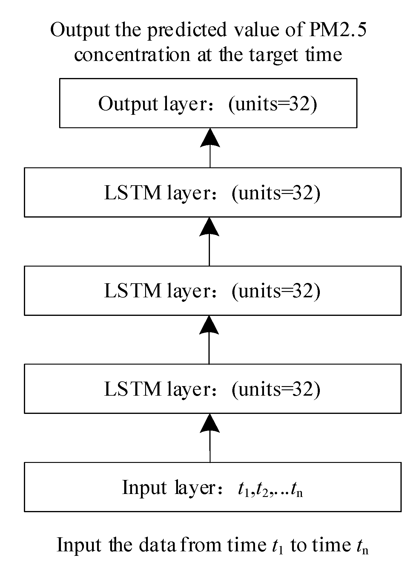
In the application scenario of this article, the D-dimensional air quality data at the latest T time is used as the input of the cyclic neural network, and the network outputs the predicted value of PM2.5 concentration at a certain time in the future. The PM2.5 concentration prediction model based on LSTM is shown in Figure 2.

Figure 2. PM2.5 concentration prediction network based on LSTM.

As shown in Figure 2, the input data is input to the LSTM layer of the first layer, and its output is a continuous complete sequence of each time step, that is, the output length of the layer is equal to the input length. The output of the first LSTM layer is the input of the second LSTM layer, and the output of the second LSTM layer is the output of the last time step of each input sequence, which learns the information of the whole sequence. Finally, in order to get a better prediction result, the output of the second LSTM layer is passed through a fully connected layer, the number of neurons in the density layer is half of that in the previous LSTM layer, and the final output layer outputs the PM2.5 concentration value at the target time.

4.2. LSTM and GRU

LSTM is widely used in natural language processing, time series prediction and other fields. Similar to general RNN, LSTM also has the chain structure of repetitive module, but the repetitive module is different from general recurrent neural network [23,24]. It has four neural network layers (standard recurrent neural network repetitive module), and its structure is shown in Figure 3.

Figure 3. LSTM Module.

Compared with the traditional LSTM model, GRU model is simpler and converges faster. Therefore, to reduce the training time of the model, GRU is used as the core repetitive unit structure of the prediction model. GRU combines the forgetting gate and input gate to form the update gate, and also integrates the unit state and hidden state. The structure of GRU is shown in Figure 4.

Figure 4. GRU network basic unit.

x_t, h_t, r_t, z_t, and ${\tilde{\mathit{h}}}_t$ are the input vector, state memory variable, update gate state, reset gate state and current candidate set state at time t, respectively. I is the identity matrix.

The mathematical description of GRU is:

$$\left\{\begin{array}{l}{\mathit{z}}_t=\sigma ({\mathit{W}}_z\cdot [{\mathit{h}}_{t-1,} {\mathit{x}}_t])\\ {\mathit{r}}_t=\sigma ({\mathit{W}}_r\cdot [{\mathit{h}}_{t-1,} {\mathit{x}}_t])\\ {\tilde{\mathit{h}}}_t=\tanh (\mathit{W}\cdot [{\mathit{r}}_t\times {\mathit{h}}_{t-1,} {\mathit{x}}_t])\\ {\mathit{h}}_t=(\mathit{I}-{\mathit{z}}_t)\times {\mathit{h}}_{t-1}+{\mathit{z}}_t\times {\mathit{h}}_t\\ {\mathit{y}}_t=\sigma ({\mathit{W}}_o\cdot {\mathit{h}}_t)\end{array}\right.$$

(8)

where W_z, W_r, W_h and W_o are the weight parameters of reset gate, update gate, candidate set, output vector y_t, input vector x_t and h_t−1;$\sigma$ is the sigmoid activation function.

The mathematical description of tanh and $\sigma$ are as follows

$$\sigma (x)=\frac{1}{1+e^{-x}}$$

(9)

$$\tanh (x)=\frac{e^x-e^{-x}}{e^x+e^{-x}}$$

(10)

4.3. Prediction of PM2.5 Concentration Based on GRA-GRU Model

The existing prediction models based on machine learning can only use the historical data of the target prediction site when predicting the PM2.5 concentration of a single site. This kind of model does not consider the regional characteristics of PM2.5 and cannot fully consider the regional effects of pollutants. To solve this problem, this paper proposes a PM2.5 concentration prediction model based on GRA-GRU model, which can not only learn the information of time dimension, but also fully consider the influence of the area around the site to be tested.

The basic idea of GRA-GRU neural network is to extract PM2.5 concentration time series of all 14 stations to form PM2.5 concentration data set $X(t)={(X_1(t),X_2(t),\dots ,X_{14}(t))}^T$, and calculate the grey correlation degree among stations through GRA, so as to get PM2.5 concentration spatial weight matrix W_s×s, where s = 14. Then, the spatial weight matrix W_s×s is multiplied by PM2.5 concentration data set X (T) to obtain a new data set with spatial weight. The calculation formula is as follows:

$$X_s(t)=W_{14\times 14}\cdot X(t)=\left[\begin{array}{cccc}0& r_{1,2}& \dots & r_{1,14}\\ r_{2,1}& 0& \dots & r_{2,14}\\ \dots & \dots & & \dots \\ r_{14,1}& r_{14,2}& \dots & 0\end{array}\right]\left[\begin{array}{c}{X}_1(t)\\ X_2(t)\\ \dots \\ X_{14}(t)\end{array}\right]$$

(11)

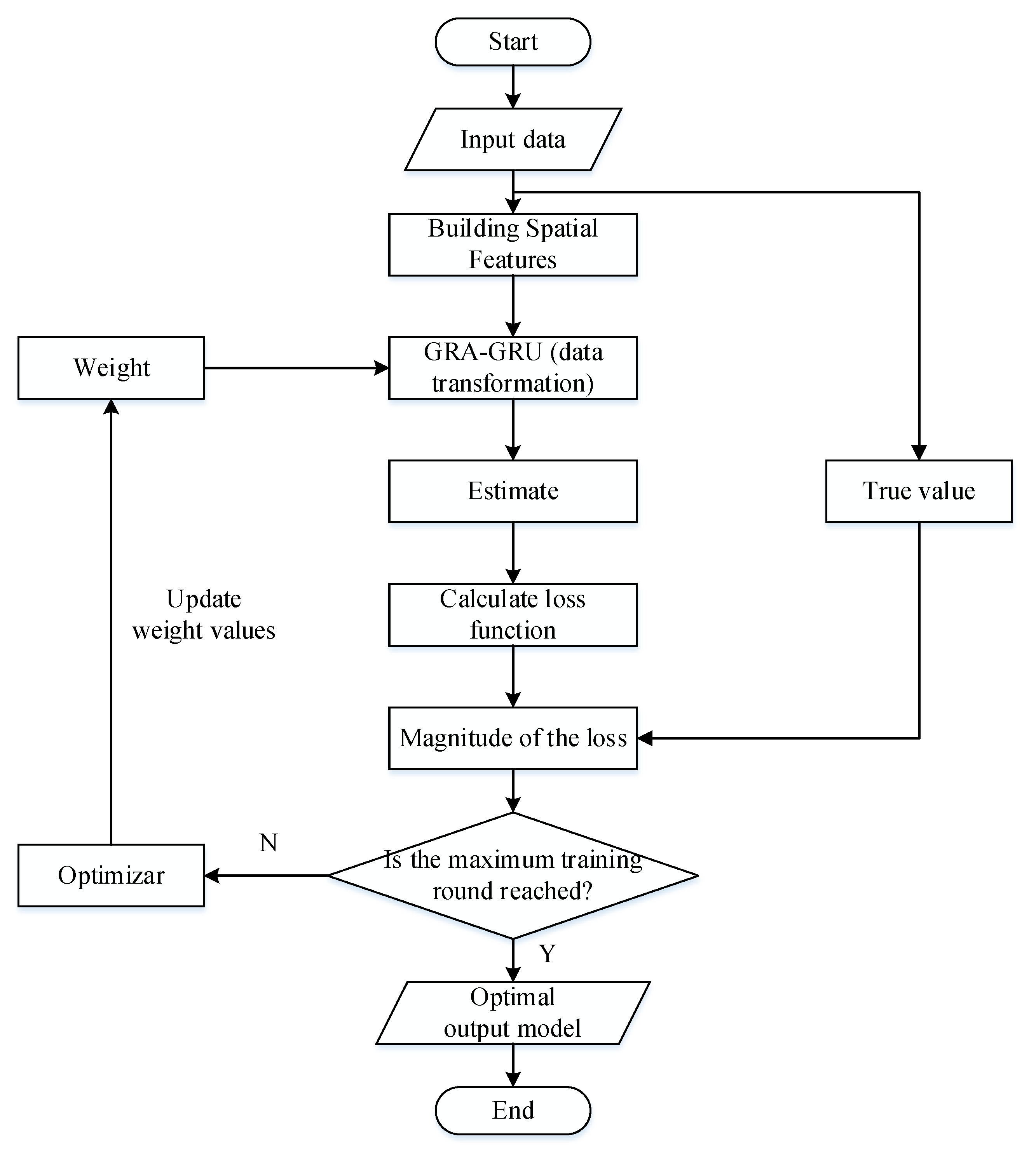
Then, X_s(t) is added to the original data set as the input of the network. Finally, the predicted value of the output of GRA-GRU neural network is compared with the real value to get the loss, and the model parameters are updated by loss back propagation. The flow chart of the GRA-GRU model algorithm is shown in Figure 5. The algorithm steps of GRA-GRU is as follows:

Figure 5. GRA-GRU prediction model.

Step 1: Input preprocessed data;

Step 2: Extract and construct the PM2.5 concentration data set X(t), and calculate the spatial feature set of Equations (1), (6) and (7);

Step 3: Obtain a new data set by splicing the spatial feature set with the original data set, and divide the new data set into training data set and test data set;

Step 4: Input the training data and calculate the predicted value $y_i$;

Step 5: Calculate the mean square error between the predicted value $y_i$ and the real value $y_i$;

Step 6: The model parameters are updated by loss back propagation;

Step 7: Repeat step 4 to step 6 until the maximum training epoch is reached;

Step 8: Verify the model on the test set;

Step 9: End.

5. Experiment and Analysis

5.1. Simulation Parameters and Environment

This paper uses 11,346 h of historical air quality data from 14 air quality monitoring stations in Changchun City from 1 August 2016, to 6 March 2020, as well as historical meteorological data of Changchun City. The data are divided into two categories: (1) Hourly observation data of 10 stations, including PM2.5 concentration, PM10 concentration, O₃ concentration, SO₂ concentration and visibility. The data are updated every 1 h. See Table 1 for details; (2) The objective analysis data of grid three-dimensional meteorological elements in Changchun area, with a spatial resolution of 1 km, is updated every 1 h, mainly including temperature, wind and relative humidity elements.

Table 1. Site Feature Vector of Input GRA-GRU Model.

Field Name	Describe
ID	Station No
PM2.5	PM2.5 concentration
PM10	PM10 concentration
SO2	sulfur dioxide concentration
O3	ozone concentration
vis	visibility
tem	visibility
win	wind speed
rh	relative humidity
prs	Average air pressure

The programming language used in this paper is Python 3.5, while TensorFlow and Keras deep learning framework are used, Pandas and Numpy are used as data preprocessing packages, the visualization package used in the experiment is Matplotlib, and the integrated development environment of the experiment is Pycharm. The training and testing of the experiment are carried out on the remote server. The main configuration of the computer used in this paper is as follows: the operating system is windows10 (64 bit); The memory size is 16 G; The processor is Intel (R) core (TM) i7-7700CPU@3.60 Hz; The disk drive is 1 TB ST1000DM010-2EP disk and 128 GB TigoSSD. According to the number of GRU layers, the root mean square error and the average absolute error reach the minimum when the number of GRU layers is 2. When the number of GRU layers exceeds 2, the error becomes larger. Therefore, the number of GRU network layers d = 2 is selected.

5.2. Loss Function and Precision Evaluation Index

Loss function, also known as objective function, is used to measure the difference between the predicted value ${\tilde{y}}_i$ and the real value $y_i$, and whether the current task is successfully completed. In this paper, mean square error (MSE) is used as the loss function, and the parameters need to be updated constantly to minimize MSE.

$$\mathrm{MSE}=\frac{1}{n}{\displaystyle \sum _{i=1}^n{(y_i-y_i)}^2}$$

(12)

In this paper, mean absolute error (MAE), root mean squared error (RMSE) and mean absolute percentage error (MAPE) are used to evaluate the prediction accuracy of the algorithm. The MAE represents the average absolute value of the deviation between all observations and the predicted value, which can avoid the problem of mutual cancellation of errors, and thus can accurately reflect the size of the actual forecast data error. The RMSE is very sensitive to the large error between the observed value and the predicted value. The MAPE is used to reflect the average level of error in the actual output data, which can avoid the problem of mutual cancellation of errors between data. The smaller the values of $e_{\mathrm{MAE}}$, $e_{\mathrm{RMSE}}$ and $e_{\mathrm{MAPE}}$, the more accurate the predicted result. The following are three kinds of error calculation formulas:

$$e_{\mathrm{MAE}}=\frac{1}{N}{\displaystyle \sum _{i=1}^N\left|y_i-{\widehat{y}}_i\right|}$$

(13)

$$e_{\mathrm{RMSE}}=\sqrt{\frac{{{\displaystyle \sum _{i=1}^N\left(y_i-{\widehat{y}}_i\right)}}^2}{N}}$$

(14)

$$e_{\mathrm{MAPE}}=\frac{1}{n}{\displaystyle \sum _{i=1}^N\left|\frac{y_i-{\widehat{y}}_i}{y_i}\right|}\times 100\%$$

(15)

where y is the observed value, $y_i$ is the predicted value and N is the test set size.

5.3. Super Parameter Selection of GRU Model

Five GRU models with different structures are tested using validation set data. The number of layers, number of hidden neurons, network parameters and errors of each structure are shown in Table 1. It can be seen from Table 2 that simply increasing the number of layers or nodes cannot reduce the error of the model. When the nodes of each layer are more than 300, the error increases significantly. When the nodes of each layer are more than 4 GRU stacks, the error of e_RMSE increases significantly. The model with 128 nodes in each layer has the smallest error and the best performance. Therefore, the GRU model of this structure is selected for the follow-up experiments.

Table 2. Error comparison among different GRU structure.

Structure	Number of Layers	Hide Node	${\mathit{e}}_{\mathbf{MAE}}/\mathbf{ug}·{\mathbf{m}}^{-3}$	${\mathit{e}}_{\mathbf{RMSE}}/\mathbf{ug}·{\mathbf{m}}^{-3}$
GRU-1	1	64	9.93	17.66
GRU-1	1	128	12.34	18.92
GRU-2	2	128	9.81	15.74
GRU-3	3	384	9.93	50.84
GRU-4	4	512	20.68	54.25

Too many training epochs will cause the model to overfit the training data and consume more time. Figure 6 shows the change of $e_{\mathrm{MAPE}}$ of training set and validation set data with the number of training iterations, and the error decreases with the increase of training iterations. When the number of iterations is more than 3000, the model is overfitting, and not only is the generalization ability not improved, but also there is a weak fluctuation. Therefore, we set the number of iterations to 3000. In addition, the learning rate of the model is set as 10⁻³, the decay rate is set as 0.95, the parameter initialization range is set as [−0.06, 0.06] and the model optimization algorithm is Adam algorithm.

Figure 6. Curve of eMAPE with epochs.

5.4. Comparison of Regional PM2.5 Concentration Prediction Models Based on LSTM and GRU

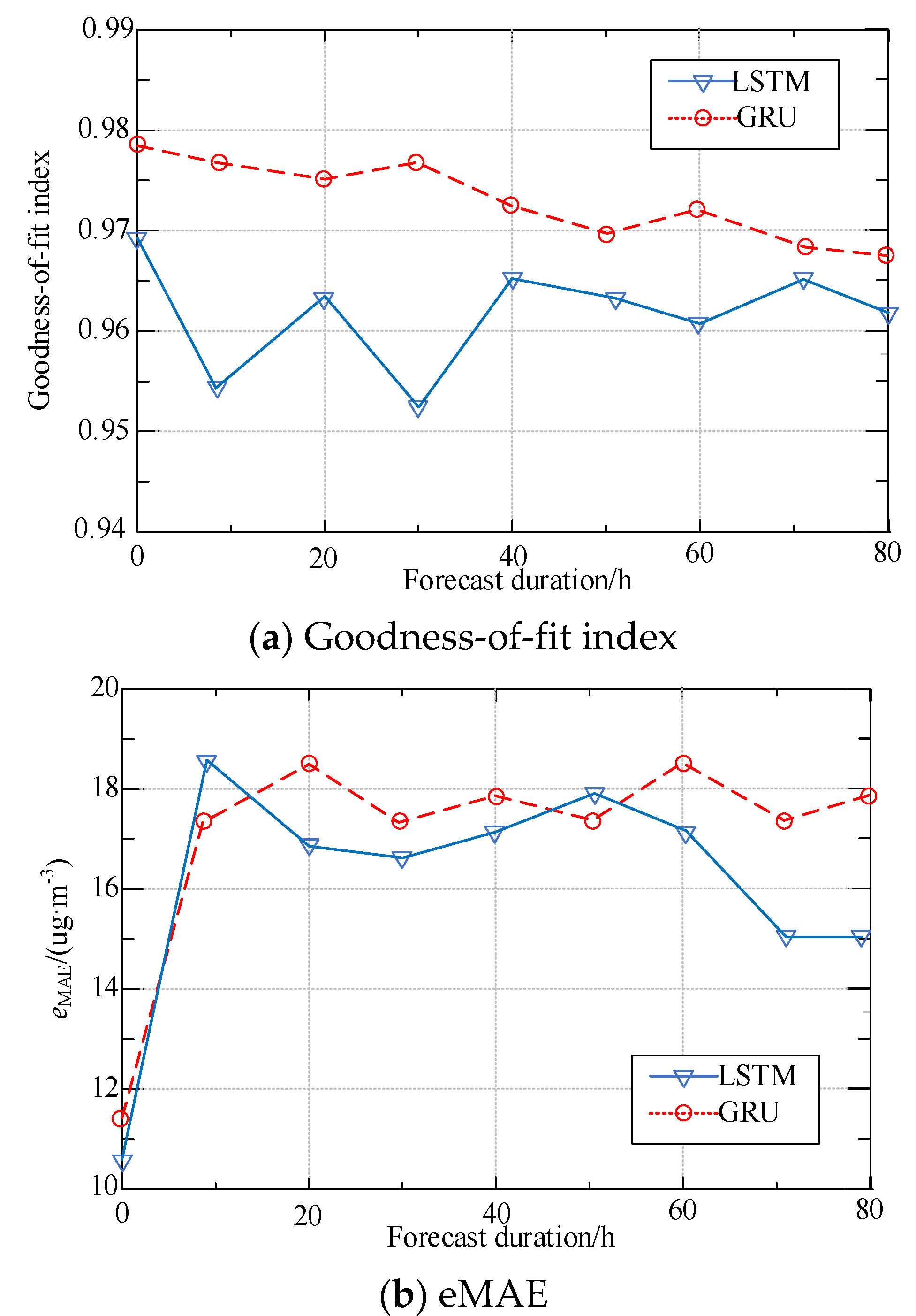
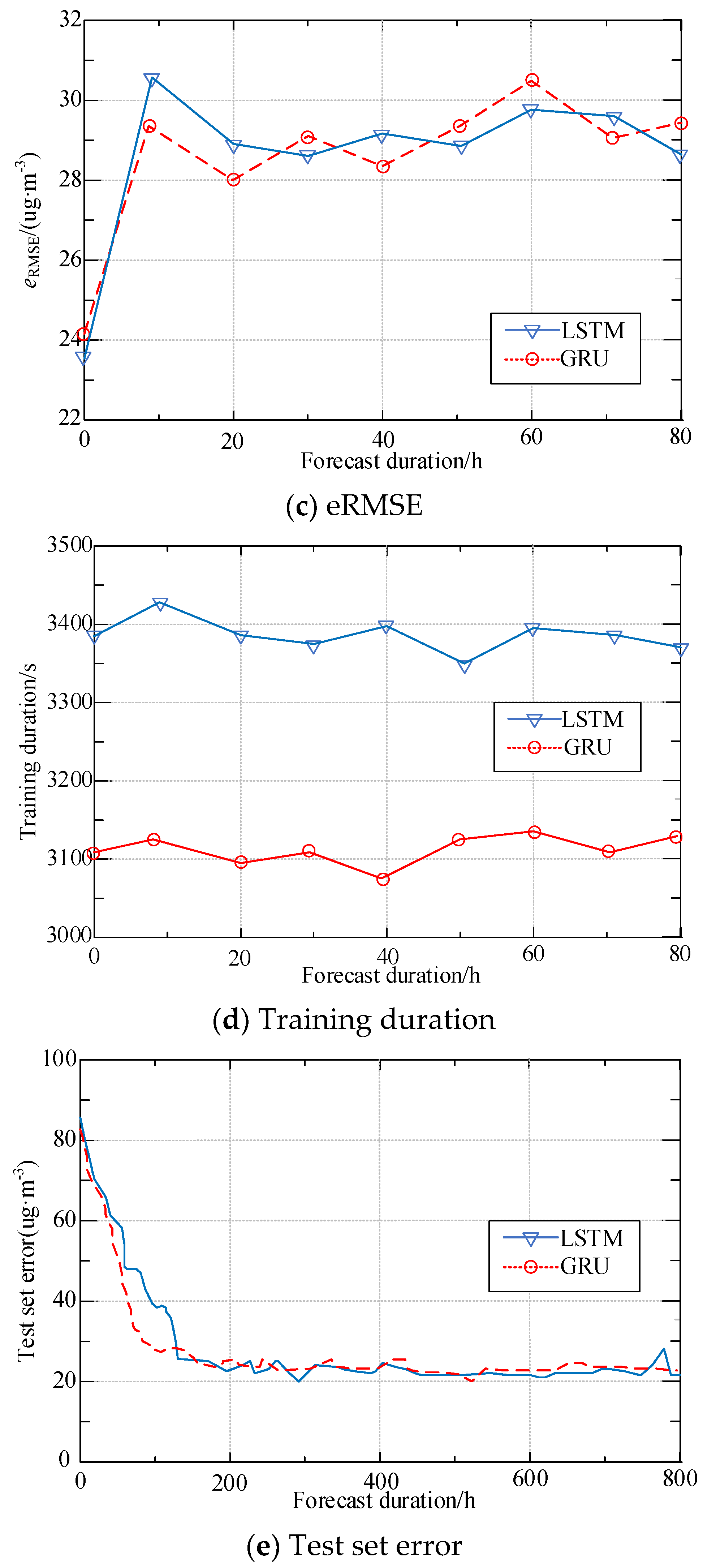
Taking meteorological factors as the model input, Figure 7 shows the prediction accuracy, required training time and convergence epoch number of PM2.5 concentration prediction model based on GRA-GRU network model proposed in this paper. It can be seen from the figure that, compared with the standard LSTM model, the prediction accuracy and prediction error of GRU model are basically the same, but the training time required is less, which indicates that GRU has an obvious effect on improving the calculation efficiency of the model. The average prediction accuracy of the statistical model is further improved and the prediction error is reduced by replacing the standard LSTM unit with GRU, synthesizing the update threshold and fusing the unit state and hidden state.

Figure 7. Comparison of regional PM2.5 concentration prediction models based on LSTM and GRU.

5.5. Performance Comparison with Other Methods

Figure 8 shows the model training error, the abscissa shows the training epochs, and the ordinate shows the training error. As can be seen from Figure 8, the training error of the prediction model based on GRA- LSTM and the prediction model based on GRA-GRU is lower than that of the prediction model based on ordinary LSTM, and the training error of the prediction model based on GRA-GRU is the lowest. On the other hand, the convergence speed of the prediction model based on GRA- LSTM and GRA-GRU is faster than that of based on ordinary LSTM, and the prediction model based on GRA- LSTM has the fastest convergence speed. When the training epochs are more than 20, the training error of GRA-LSTM is not significantly reduced, which shows that the effect of reducing the number of parameters and accelerating the convergence speed by convolution neural network is obvious.

Figure 8. Training Loss.

Table 2 shows the $e_{\mathrm{RMSE}}$ and $e_{\mathrm{MAE}}$ values of LSTM [24], FAA-LSTM [26], CNN-LSTM [28] and GRA-GRU. It can be seen from Table 3 that the prediction effect based on LSTM model is the worst, while the indicators of the prediction model based on GRA-GRU all reach the ideal situation, which indicates that the neural network with cyclic structure can learn the long-term dependence information in the time series, and adding spatial features into the data helps to improve the prediction accuracy of PM2.5 concentration. The prediction model based on FAA-LSTM is very close to the prediction model based on GRA-GRU, and the prediction model based on GRA-GRU is better because FAA-LSTM improves the convergence speed and sacrifices part of the performance.

Table 3. Comparison of prediction accuracy of four models.

Algorithm	${\mathit{e}}_{\mathbf{RMSE}}/\mathbf{ug}·\mathbf{m}{\mathbf{m}}^{-3}$	${\mathit{e}}_{\mathbf{MAE}}/\mathbf{ug}·\mathbf{m}{\mathbf{m}}^{-3}$
LSTM	23.77	17.83
FAA- LSTM	20.16	15.25
CNN-LSTM	19.78	14.15
GRA-GRU	18.32	13.54

6. Conclusions

This paper uses Changchun City as the experimental research area and GRA-GRU as the main network structure to construct a regional PM2.5 concentration prediction model to simulate the temporal change characteristics of regional PM2.5 concentration with various predictive factors, thereby improving the PM2.5 concentration prediction accuracy. We comprehensively analyze the correlation between various meteorological elements such as temperature, relative humidity, precipitation, wind, visibility and PM2.5 concentration, and calculate the correlation coefficient. Secondly, the spatial weight matrix is used to extract the spatial relationship of the original data, so that the model can not only learn the information of the time dimension, but also fully consider the influence of the area around the site to be tested.

However, the proposed method is not perfect, and the following two problems need to be overcome. The first is the selection of meteorological factors. There are some factors that are difficult to obtain and quantify, such as national policies, major activities and emergencies, which will lead to changes in PM2.5 concentration. Therefore, more source data need to be collected in future research. The second is to adjust the parameters of the GRA-GRU model and study the impact of upper air meteorological factors on the prediction results to improve the quality of prediction data. In the follow-up study, the abovementioned two aspects will be considered.

References

1. Qin, Q.; Xu, X.; Dai, Q.; Ye, K.; Wang, C.Y.; Huo, X. Air pollution and body burden of persistent organic pollutants at an electronic waste recycling area of China. Environ. Geochem. Health 2019, 41, 93–123. [Google Scholar] [CrossRef] [PubMed]
2. Wang, H.; Sun, Y.Q.; Zhang, M.; Liu, W.J.; Yang, L.; Zhou, X.W. Adsorption ability of air pollutants by indigenous tree species in ta-pieh mountains. Fresenius Environ. Bull. 2019, 28, 2908–2915. [Google Scholar]
3. Celiktas, V.; Otu, H.; Duzenli, S.; Alharby, H.; Bamagoos, A.; Islam, M.S.; Hossain, A.; Sabagh, A.E. Traffic-induced air pollution effects on physio-biochemical activities of the plant eucalyptus camuldensis. Fresenius Environ. Bull. 2019, 28, 9373–9378. [Google Scholar]
4. Tolis, E.I.; Panaras, G.; Douklias, E.; Ouranos, N.; Bartzis, J.G. Air quality measurements in a medium scale athletic hall: Diurnal and I/O ratio analysis. Fresenius Environ. Bull. 2019, 28, 658–665. [Google Scholar]
5. Gonzalez-Enrique, J.; Turias, I.J.; Jesus Ruiz-Aguilar, J.; Antonio Moscoso-Lopez, J.; Jerez-Aragones, J.; Franco, L. Estimation of NO2 concentration values in a monitoring sensor network using a fusion approach. Fresenius Environ. Bull. 2019, 28, 681–686. [Google Scholar]
6. Afridi, S.G.; Islam, N.; Shams, D.F.; Shams, S.; Khan, A.; Shah, M.; Khan, W.; Shah, M.; Islam, M.; Iqbal, A. Assessment of air pollution tolerance of selected trees and crop species using biochemical and physiological analyses. Fresenius Environ. Bull. 2019, 28, 4805–4810. [Google Scholar]
7. Dai, L.; Zhang, C.; Lei, M. Dynamic forecasting model of short-term PM2.5 concentration based on machine learning. J. Comput. Appl. 2017, 37, 3057–3063. [Google Scholar]
8. Karadirek, I.E.; Aktas, K.; Topkaya, B. Environmental pollution of the mediterranean sea: Evaluation of research activities in the mediterranean sea countries. Fresenius Environ. Bull. 2019, 28, 867–872. [Google Scholar]
9. Duzenli, T.; Alpak, E.M.; Yilmaz, S. Children’s imaginations about environment and their perceptions on environmental problems. Fresenius Environ. Bull. 2019, 28, 9798–9808. [Google Scholar]
10. Xiang, Z.; Azam, M.; Islam, T.; Zaman, K. Environment and air pollution like gun and bullet for low income countries: War for better health and wealth. Environ. Sci. Pollut. Res. 2015, 23, 3641–3657. [Google Scholar]
11. Yuan, G.H.; Yang, W.X. Evaluating China’s air pollution control policy with extended AQI indicator system: Example of the Beijing-tianjin-hebei region. Sustainability 2019, 11, 939. [Google Scholar] [CrossRef] [Green Version]
12. O’Donnell, M.J.; Fang, J.; Mittleman, M.A.; Kapral, M.K.; Wellenius, G.A. Fine particulate air pollution (PM2.5) and the risk of acute ischemic stroke. Epidemiology 2011, 22, 422–432. [Google Scholar] [CrossRef] [PubMed] [Green Version]
13. Campolim, C.M.; Weissmann, L.; Ferreira, C.K.d.O.; Zordão, O.P.; Dornellas, A.P.S.; Castro, G.D.; Zanotto, T.M.; Boico, V.F.; Quaresma, P.G.F.; Lima, R.P.A.; et al. Short-term exposure to air pollution (PM2.5) induces hypothalamic inflammation, and long-term leads to leptin resistance and obesity via Tlr4/Ikbke in mice. Sci. Rep. 2020, 10, 10160. [Google Scholar] [CrossRef] [PubMed]
14. Fong, K.C.; Bell, M.L. Do fine particulate air pollution (PM2.5) exposure and its attributable premature mortality differ for immigrants compared to those born in the United States? Environ. Res. 2021, 196, 110387. [Google Scholar] [CrossRef] [PubMed]
15. Wagner, D.R.; Brandley, D.C. Exercise in thermal inversions: PM2.5 air pollution effects on pulmonary function and aerobic performance. Wilderness Environ. Med. 2020, 31, 16–22. [Google Scholar] [CrossRef] [Green Version]
16. Kushwaha, M.; Upadhya, A.; Savio, E.; Sreekanth, V.; Asundi, J.; Apte, J.; Marshall, J. Mobile-monitoring of Black Carbon and PM2.5 air pollution data only approach from Bangalore, India. Environ. Epidemiol. 2019, 3, 200–221. [Google Scholar]
17. Schwarz, J.; Pokorna, P.; Rychlik, S.; Skachova, H.; Vlcek, O.; Smolik, J.; Zdimal, V.; Hunova, I. Assessment of air pollution origin based on year-long parallel measurement of PM2.5 and PM10 at two suburban sites in Prague, Czech Republic. Sci. Total Environ. 2019, 664, 1107–1116. [Google Scholar] [CrossRef]
18. Chen, R.; Wang, X.; Meng, X.; Hua, J.; Zhou, Z.; Chen, B.; Kan, H. Communicating air pollution-related health risks to the public: An application of the Air Quality Health Index in Shanghai, China. Environ. Int. 2013, 51, 168–173. [Google Scholar] [CrossRef]
19. Chen, J.; Lu, J.; Avise, J.C.; DaMassa, J.A.; Kleeman, M.J.; Kaduwela, A.P. Seasonal modeling of PM2.5 in California’s San Joaquin Valley. Atmos. Environ. 2014, 92, 182–190. [Google Scholar] [CrossRef]
20. Wu, Q.Z.; Xu, W.S.; Shi, A.J.; Li, Y.T.; Zhao, X.J.; Wang, Z.F.; Li, J.X.; Wang, L.N. Air quality forecast of PM10 in Beijing with Community Multi-scale Air Quality Modeling (CMAQ) system: Emission and improvement. Geosci. Model. Dev. 2014, 7, 2243–2259. [Google Scholar] [CrossRef]
21. Wang, T.; Jiang, F.; Deng, J.; Shen, Y.; Fu, Q.; Wang, Q.; Fu, Y.; Xu, J.; Zhang, D. Urban air quality and regional haze weather forecast for Yangtze River Delta region. Atmos. Environ. 2012, 58, 70–83. [Google Scholar] [CrossRef]
22. Zhao, J.C.; Deng, F.; Cai, Y.Y.; Chen, J. Long short-term memory—Fully connected (LSTM-FC) neural network for PM2.5 concentration prediction. Chemosphere 2019, 220, 486–492. [Google Scholar] [CrossRef] [PubMed]
23. Vidushi, C.; Anand, D.; Vijayanand, K. Time series based LSTM model to predict air pollutant’s concentration for prominent cities in India. In Proceedings of the 1st International Workshop on Utility-Driven Mining, London, UK, 20 August 2018. [Google Scholar]
24. Thaweephol, K.; Wiwatwattana, N. Long short-term memory deep neural network model for PM2.5 forecasting in the Bangkok urban area. In Proceedings of the 17th International Conference on ICT and Knowledge Engineering (ICT&KE), Bangkok, Thailand, 20–22 November 2019. [Google Scholar]
25. Lu, G.B.; Yu, E.P.; Wang, Y.J.; Li, H.L.; Cheng, D.P.; Huang, L.; Liu, Z.Y.; Manomaiphiboon, K.; Li, L. A novel hybrid machine learning method (OR-ELM-AR) used in forecast of PM2.5 concentrations and its forecast performance evaluation. Atmosphere 2021, 12, 78. [Google Scholar] [CrossRef]
26. Liu, D.-R.; Hsu, Y.-K.; Chen, H.-Y.; Jau, H.-J. Air pollution prediction based on factory-aware attentional LSTM neural network. Computing 2020, 103, 75–98. [Google Scholar] [CrossRef]
27. Soh, P.-W.; Chang, J.-W.; Huang, J.-W. Adaptive deep learning-based air quality prediction model using the most relevant spatial-temporal relations. IEEE Access 2018, 6, 38186–38199. [Google Scholar] [CrossRef]
28. Huang, C.-J.; Kuo, P.-H. A deep CNN-LSTM model for particulate matter (PM2.5) forecasting in smart cities. Sensors 2018, 18, 2220. [Google Scholar] [CrossRef] [Green Version]
29. Chang, S.-W.; Chang, C.-L.; Li, L.-T.; Liao, S.-W. Reinforcement Learning for Improving the Accuracy of PM2.5 Pollution Forecast Under the Neural Network Framework. IEEE Access 2019, 8, 9864–9874. [Google Scholar] [CrossRef]
30. Lee, C.; Lee, K.; Kim, S.; Yu, J.; Jeong, S.; Yeom, J. Hourly Ground-Level PM2.5 Estimation Using Geostationary Satellite and Reanalysis Data via Deep Learning. Remote Sens. 2021, 13, 2121. [Google Scholar] [CrossRef]
31. Satria, H.; Soekirno, S. Design of PM2.5 and PM10 measuring instruments for analysis of air pollution distribution patterns in the dramaga area based on internet of things. J. Phys. Conf. Ser. 2021, 1816, 012053. [Google Scholar] [CrossRef]