Abstract
This study proposes a method that is used for the nondestructive detection of copper content in corn leaves, which is achieved via visible–near infrared spectroscopy. In this paper, we collected the visible–near infrared spectral data of corn leaves that were planted in soils undergoing different gradients of heavy metal copper stress. Then, a preliminary pretreatment was carried out to obtain the original spectrum (OS), the continuous removal spectrum (CR), and the derivative of ratio spectroscopy (DRS). Singular value decomposition was used for spectral denoising. The characteristic bands corresponding to the OS, CR, and DRS were determined using correlation analysis, as well as mutual information. Based on training the extreme gradient boosting tree (XGBoost) predictive model using feature bands, the copper content in corn leaves was predicted, and a comparative analysis was conducted with the commonly used partial least squares regression (PLSR) model in regression analysis. The results showed that the accuracy of the PLSR and XGBoost models, which were established with CR and DRS, were higher than that of the OS, among which the DRS model had the highest accuracy. For the validation set in the PLSR model, the coefficient of determination (R2) was 0.72, the root mean square error (RMSE) was 1.21 mg/kg, and the residual predictive deviation (RPD) was 1.89. For the validation set in the XGBoost model, the R2 was 0.86, the RMSE was 0.86 mg/kg, and the RPD was 2.66. At the same time, the spectral data of the field-planted corn near a mining area were selected to test the robustness of the model. Among them, the DRS had a higher accuracy in the XGBoost model, where its R2 was 0.51, its RMSE was 0.86 mg/kg, and its RPD was 1.45, thus indicating that the model can better predict the copper content in corn leaves and that the model has a higher robustness, which could provide new ideas for the prediction of heavy metal content in crops.
1. Introduction
With the development of the industry and the progress of technology, the problem of environmental pollution has become increasingly prominent, among which heavy metal pollution has received widespread attention [1,2]. Heavy metals left in the soil for anthropogenic reasons are nondegradable. When the concentration of heavy metals in the soil exceeds the environmental background value, the soil quality is seriously reduced, which eventually leads to heavy metal stress on the crops planted [3,4]. Copper is one of the elements required for the growth of crops, albeit when it is within a certain range. However, the development of the crops can also be affected when copper levels exceed a certain concentration [5]. It poses a serious threat to human health as soon as it enters the human body through the ecosystem or food chain [6]. Bawa’s research revealed that crops that were treated with pesticides containing heavy metals and crops irrigated with water from drilling sources exhibited copper levels that exceeded the permissible limits. In addition, the consumption of crops that exceed the copper limit poses a potential risk of developing cancer [7]. Corn is one of the most widely grown crops in the world, second only to rice in terms of production [8]. Various types of plasma membrane structures are damaged to varying degrees, and the activity of enzymes in the corn plant is reduced when corn is subjected to heavy metal stress, thus affecting physiological and biochemical parameters, which leads to a failure in the normal growth of corn [9,10]. Therefore, the issue of monitoring heavy metals such as copper in corn is of great importance.
Hyperspectral remote sensing is currently at the forefront of remote sensing technology; the technology utilizes multiple narrow electromagnetic wave bands to acquire crucial information from research targets [11,12]. Hyperspectral data contain abundant spatial, radiometric, and spectral information, thereby enabling the detection of substances that were previously undetectable in broadband remote sensing [13]. Instruments such as prism spectrometers, grating spectrometers, Fourier transform spectrometers, and spectrophotometers can be used to obtain the hyperspectral data of research objects [14]. Among these, portable land cover spectrometers possess several advantages, including strong portability, real-time measurement capabilities, multifunctionality, high accuracy, and real-time data processing. These features make them indispensable tools in land cover research, environmental monitoring, agricultural management, and other related fields [15].
The traditional measurement of heavy metal copper content in crops is not only time-consuming and complicated but also damaging to crops, and it can easily cause secondary pollution to the environment [16]. Hyperspectral remote sensing has a wide range of applications in monitoring heavy metal content. Zhang et al. [17] developed an inverse model for heavy metals with a high prediction accuracy, and it is based on the spectral data of cultivated land in major grain producing areas. The model uses fixed-effect variable coefficients based on least squares estimation. Zhang et al. [18] proposed a heavy metal stress sensitivity index, and they used the random forest algorithm to establish a multitemporal monitoring model for the detection of heavy metal stress levels in rice at different stages (which are based on rice hyperspectral data). Azadi [19] extracted sensitive bands in the leaf spectral data of grape seedlings using the partial least squares technique, and they applied multiple linear regression and support vector machine regression to predict the content of five heavy metals in grape seedlings. Zhong et al. [20] employed a genetic algorithm that optimizes a partial least squares regression (GA-PLSR) model to indirectly estimate the concentrations of soil heavy metals, specifically cadmium (Cd) and arsenic (As), and this was achieved by utilizing the hyperspectral data obtained from wheat leaves. Liu et al. [21] identified characteristic variables by conducting a correlation analysis and utilizing multiple linear regression models. Additionally, they developed a vegetation index known as HMSVI to estimate the concentrations of heavy metals, specifically cadmium (Cd), arsenic (As), and lead (Pb), in both peach leaves and soil. The above studies provide a basis for hyperspectral techniques in the context of heavy metal content monitoring. However, there are three shortcomings, i.e., there are more conventional prediction models, there is a low accuracy in the prediction results, and the robustness of the models is unknown.
Different spectral transformation methods can not only highlight spectral characteristics but also improve data quality. Continuum removed (CR) is a typical spectral transformation method which can enhance the absorption and reflection characteristics of the spectral profile [22]. Chen et al. [23] processed the hyperspectral reflectance data of 26 soil samples from oil recovery operation areas in China, and they found that the continuum removed method could be used to improve the correlation between spectral reflectance and petroleum hydrocarbon content, which effectively improved the sensitivity of the spectra to petroleum hydrocarbons. The derivative of ratio spectroscopy (DRS) is a transformation method that was introduced from chemical research to the hyperspectral field. This method can eliminate the influence of interference components, as well as effectively analyze multicomponent mixed systems [24]. Wang et al. [25] analyzed the trend (and obtained better results) during the corrosion process of ettringite, which is a product of concrete corrosion, by using the derivative of ratio spectroscopy through the hyperspectral data of concrete.
An appropriate regression model can establish a closer relationship between the predicted target and the spectral data. The extreme gradient boosting tree (XGBoost) method can fit the characteristic elements of nonlinear relationships. It has been proven that machine learning models have a shorter training time and higher efficiency in processing data [26]. Tian et al. [27] estimated the above-ground biomass of mangrove forests in the south subtropical region of China using eight machine learning models, and they found that the XGBoost model had a fast training speed and high accuracy. Partial least squares regression (PLSR), a widely employed regression analysis technique, demonstrates substantial advantages in handling high-dimensional data, addressing multicollinearity, and extracting relevant information. It has been extensively applied across various domains, yielding favorable outcomes [28,29]. Consequently, this study has opted to undertake a comparative analysis between PLSR and the XGBoost model.
In previous studies, researchers have discovered that the characteristic bands present in corn leaf spectra can be effectively utilized in conjunction with PLSR and XGBoost models to achieve precise predictions of the copper content in corn leaves, particularly those pertaining to heavy metal concentration. In order to reduce the interference of external uncertainties, this study was conducted in a laboratory with controllable conditions. In this study, corn leaves under different gradients of copper stress were used as the research object, and their visible–near infrared original spectrum (OS) was collected by an ASD FieldSpec 4 portable ground object spectrometer. CR and DRS spectral transformation, as well as singular value decomposition (SVD) denoising, were performed. Then, correlation analysis (CA) and mutual information (MI) were used to determine the characteristic bands corresponding to OS, CR, and DRS. The prediction model of the copper content in corn leaves, which is based on PLSR and XGBoost, was established for the selected characteristic bands. At the same time, the spectral data of field-planted corn near a mining area were selected to test the robustness of the model. After comparing the predictive accuracy and robustness of the XGBoost and PLSR models, this study aimed to identify an optimal predictive model for forecasting copper content in corn leaves. This research provides a basis for the rapid detection of copper in corn plants and the management of heavy metal pollution in contaminated areas.
2. Materials and Methods
2.1. Experimental Design
Corn plants under different gradient copper stress were cultured in a plant culture laboratory. The type of corn seeds selected was “Minuo 8”. A CuSO4·5H2O solution with the respective stress gradients of 50, 100, 150, 200, 300, 400, 600, 800, and 1000 mg/kg were added into uncontaminated natural soil as a copper stress reagent for corn plants. Three parallel test sample groups were set up for different copper stress gradients. At the same time, in order to compare the experimental results, three groups of blank control groups were set up, which were marked as CK1, CK2, and CK3, and which did not include heavy metal reagents. The indoor temperature of the cultivation site was controllable, the water and gas environment was suitable, the nutrient elements were sufficient, and the light, water, acid, and alkali conditions were consistent.
Spectral data acquisition was performed in a dark room without the influence of light. To address the situation that the copper content may vary at different locations for the same corn plant leaves, the top leaves were used as new leaves, the middle leaves as middle leaves, and the lower leaves as old leaves when the corn plant samples were grown to the cob stage. The ASD FieldSpec 4 portable ground object spectrometer, with a band range of 350–2500 nm, was used to collect the visible–near infrared spectral data of the old, middle, and new leaves of the corn plants with different copper stress gradients (which were labeled as Cu(50)1-O, Cu(50)1-M, Cu(50)1-N, Cu(1000)3-O, Cu(1000)3-M, and Cu(1000)3-N, with a total of 90 sets of sample data). Through using a halogen lamp with a power of 235 W as a simulated light source for the indoor experiments, each of the leaves of the groups to be measured were laid flat on a black velvet cloth on the experimental table, and the distance between the light source and the sample under test was set to 60 cm. Moreover, the field of view of the light source was set to 15°, and a probe with a field of view of 25° was used to collect data at a distance of 10 cm perpendicular to the surface of the leaves. In order to ensure that the samples were measured completely within the field of view of the spectrometer probe, the diameter of each of the leaves in the groups of leaf samples was made larger than 5 cm, and this was based on the probe’s field of view and the measurement height. To mitigate the potential impact of the surrounding environment, it was recommended that the personnel conducting the spectral measurements wear darker shade attire. The spectrometer was warmed up for 30 min before the formal measurement was started. The spectrometer was calibrated using a standardized whiteboard. To enhance the universality of the measured spectral data for corn leaves, the spectral reflectance of each sample was captured at three distinct positions, with each position being measured three times. The average value derived from the nine spectral reflectance measurements was utilized as the actual spectral reflectance data for each sample in subsequent experimental investigations.
The corn leaves that underwent spectral data collection were washed, dried, crushed, and microwave digested, and the copper content of the corn leaves was determined by inductively coupled plasma emission spectrometry (ICP-OES) (which was undertaken for the validation of the study results).
2.2. Data Preprocessing Methods
CR is a spectral preprocessing method that highlights the absorption and reflection characteristics of a spectral profile, as well as normalizes the reflectance. By means of calculating the maximum extreme value point on the spectral curve as an endpoint of the envelope, as well as by calculating the slope of the line connecting the point with each extreme value point in the wavelength growth direction and taking the maximum slope point as the next endpoint of the envelope, the endpoints are all cycled through to form the envelope of the spectral curve. In addition, the reflectance value of the actual spectral curve is divided by the reflectance value of the corresponding band on the envelope in order to obtain the result of the original spectral curve after removing the envelope, as shown in Equations (1) and (2).
where Si is the envelope removal value of band i; K is the slope between the beginning and end points of the maximum value; ρi is the original spectral reflectance of band i; ρs and ρe are the original spectral reflectance of the beginning and end points of the maximum value, respectively; and λs and λe are the band values corresponding to ρs and ρe.
DRS refers to a method that can operate the ratio of two continuous spectral curves according to the band to obtain a ratio spectrum, and this can then be used to obtain the derivative of the above ratio spectrum, which is processed to obtain a derivative of ratio spectroscopy. This method is a spectral transformation method that is based on a linear mixture model which can suppress the spectral characteristics as denominators and highlight the influence of molecular spectra. In the linear spectral mixing model, the spectral reflectance of a certain band is expressed as a linear combination of the reflectance of each fundamental end element group that accounts for a certain proportion, and the proportion is determined by the abundance of the relevant end element group spectra. Based on this, the linear spectral mixing model is established, as shown in Equation (3).
where i = 1, 2, 3, …, n denotes the spectral channels; k = 1, 2, 3, …, m denotes the end element components; Ak is the abundance of each end element component in the mixture; Rk(λi) is the reflectance of the kth end element at the λi band; and ξ(λi) is the error term and total error term of the ith spectral channel. When the mixed spectrum contains two different components, the simplified linear spectral mixing model is as shown in Equation (4), without considering the effect of errors.
When dividing the reflectance spectrum of the second component on both sides of Equation (4) simultaneously, the following equation is obtained, as shown in Equation (5):
When deriving λi on both sides of Equation (5) simultaneously, the following equation is obtained, as shown in Equation (6):
where is the error compensation term, including nonlinear mixing factors as well as noise, etc. It can be seen from Equation (6) that the spectral data after the ratio derivative transformation are only related to the content of the first component A1 and not to the abundance as a divisor component. The simplicity of the DRS algorithm avoids the complex operation of exhaustive iterations in the least squares method, and it simplifies the process of unmixing mixed spectra.
SVD is a matrix decomposition method that is often used for noise removal or data compression. SVD means that there are always orthogonal matrices U ∈ Rn×n and V ∈ Rm×m for any matrix A ∈ Rn×m, such that the followings holds:
where S = [diag(σ1, σ2, …, σj),O]; j = min(n,m),O is the zero matrix; and σ1 ≥ σ2 ≥ … ≥ σj ≥ 0 is the singular value of matrix A. Let U = [u1,u2, …, un] be the set of left singular vectors corresponding to a singular value, and let V = [v1,v2, …, vm] be the set of right singular vectors corresponding to a singular value. Where there is ui ∈ Rn×1 and vi ∈ Rm×1, then the matrix A can be rewritten as the following equation shown in Equation (8):
Let Ai = uiσiviT(i = 1,2, …, j). According to the results of previous studies, it is known that the singular value of the matrix is the most important information in the matrix, the singular value decays faster from large to small, and the sum of the first 10% or even 1% of the singular values accounts for more than 90% of the sum of all of the singular values. In order to not miss the characteristics, let the sum of the singular values of the first w components be 90% of the sum of the singular values, and also select the first w components for reconstruction to obtain the approximate matrix shown in Equation (9). According to Equation (9), it can be seen that the reconstructed matrix retains the important characteristics on the basis of the original matrix, as well as removes the noise effects.
The OS, CR, and DRS were the basic data of this study.
2.3. Characteristic Band Extraction Methods
The hyperspectral data band interval is small, the data volume is large, and not all the band data are closely related to the model, so there is a certain redundancy phenomenon. If all of the band data are used to build the inverse model, it will not only affect the efficiency but also reduce the model accuracy, so it is necessary to extract the characteristic bands related to the model before modeling.
CA can respond to the degree of correlation between the data. Pearson correlation analysis was performed by band-by-band correlation analysis between the spectra of the corn leaves subjected to different degrees of copper stress and measured copper content, and the correlation coefficient of each band with copper content was calculated. The band that passed the p = 0.01 significance test was taken as the initial selection of the characteristic band. The correlation coefficient formula is shown in Equation (10).
where C is the correlation coefficient between the spectra of the corn leaves with different copper stresses and measured copper content; n is the number of samples; Xi is the spectral data of the ith sample; Yi is the actual copper content of the ith sample; is the mean value of Xi; and is the mean value of Yi.
MI can not only indicate the degree of interdependence of two random variables, but it can also determine the degree of association between them. When the MI is 0, it means that the two are mutually independent variables, and the larger the value of the MI, the higher the degree of association between them. The MI of two discrete random variables T and L can be expressed by Equation (11).
where p(t, l) indicates the probability of T = t, wherein L = l is occurring simultaneously; p(t) is the probability of T = t occurring; and p(l) is the probability of L = l occurring. The elemental concentration of the substance is related to certain bands in the spectrum, the noise data have no relationship with the elemental concentration, and the use of mutual information to remove the data independent from each other and the elemental concentration will play a role in quantitative analysis. In this study, the characteristic bands initially selected by correlation analysis were analyzed by mutual information with the measured copper content, and the top 10 bands with the highest MI values were selected as the characteristic bands for model construction.
2.4. Prediction Model and Evaluation Indexes
PLSR is a regression analysis of component variables that is obtained by combining principal component analysis and typical correlation analysis. It can analyze data with strong covariance, the containment of noise, and multiple independent variables. In order to obtain a relatively reliable regression analysis model, the number of principal components was integrated using the training set with a 9-fold cross-validation estimation of the root mean square error of prediction (RMSEP) and cumulative contribution rate (CCR) when building the partial least squares regression model. The current number of principal components is the optimal number of principal components when the RMSEP approaches 0 and tends to be stable, as well as when the CCR reaches 0.99 and tends to be stable. The construction of the PLSR model in this study was conducted in MATLAB (version R2023b).
XGBoost is an integrated learning method that is implemented on the basis of a gradient boosting decision tree, and it can fit the characteristic elements of nonlinear relationships, it can support parallelization and positive regularization, and it has many advantages such as a fast training speed and high efficiency in processing data. The construction of the XGBoost model in this study was conducted in Python (version 3.12.1).
The evaluation index of the model includes the following three kinds: root mean square error (RMSE), coefficient of determination (R2), and residual predictive deviation (RPD). RMSE represents the difference between the predicted value and the true value. The closer the RMSE is to 0, the higher the prediction accuracy of the model. R2 indicates how well the predicted value fits the true value, and the closer R2 is to 1, the better the fit of the model. The RPD indicates the predictive ability of the model, and an RPD of >2.0 indicates a strong predictive ability of the model; moreover, when 2.0 > RPD > 1.4, then it indicates an average predictive ability of the model, and when the RPD is <1.4, it indicates a poor predictive ability of the model [30]. The RMSE, R2, and RPD were calculated as follows:
where yi and denote the true value and the corresponding predicted value, respectively; denotes the mean of the true values of all of the samples; and n denotes the number of samples.
3. Results
3.1. Data Preprocessing
The copper content of corn leaves measured using ICP-OES under the same stress gradient should be in the same range, but there may be some outliers due to other uncontrollable factors such as the environment. The quartile method was used to calculate the range of copper content in the corn leaves for each stress gradient, and outliers were marked as shown in Figure 1.
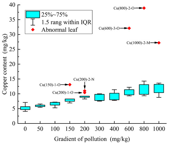
Figure 1.
Normal range and abnormal value of the copper content in leaves in each stress gradient.
The overall copper content in the corn leaves increased gradually with increasing stress gradients, as shown in Figure 1, and 6 of the 90 sets of sample data exceeded the normal range of copper content for the corresponding gradients. All abnormal values that fell outside of the normal range were eliminated. Then, the copper content of each group of leaves was calculated using the mean values of the old, middle, and new leaves of each gradient after excluding outliers, as shown in Table 1. For each copper stress gradient, three sets of parallel experiments were conducted. In this study, the first and third parallel experimental groups were used as the model’s training set, and the second set of parallel experiments was used as the model’s validation set. The validation set samples are indicated by * in Table 1. The measured copper content of the leaves in Table 1 was used in the subsequent calculations.

Table 1.
The copper content of the leaves under different stress gradients.
Figure 2 depicts the original spectral curves of the corn leaves with different gradients of copper stress. It can be seen from the figure that the spectral curves of all samples showed the spectral characteristics of typical vegetation. Due to varying degrees of copper stress, the spectral reflectance of the corn leaves exhibited distinct variations. In the vicinity of the chlorophyll absorption peaks at 450 nm and 650 nm, the spectral reflectance of the corn leaves increased with higher copper content, thus suggesting a reduction in chlorophyll content. Similarly, the reflectance near the green light reflection peak at 540 nm showed an upward trend with increased copper content, thereby indicating a decrease in the greenness of the corn leaves. In the spectral range of 780–1300 nm, which corresponded to the internal structure of corn leaves and was near the water absorption peaks of 1400 nm and 1900 nm, significant differences in reflectance were observed. These differences implied that copper affects the internal structure and water content of corn leaves, although no clear regularity was evident, thus making a direct prediction of the copper content challenging when using the original spectrum alone. Therefore, employing spectral transformation processing becomes necessary to enhance spectral characteristics and to capture the variations in the spectral curves of the corn leaves when under different copper stress gradients.
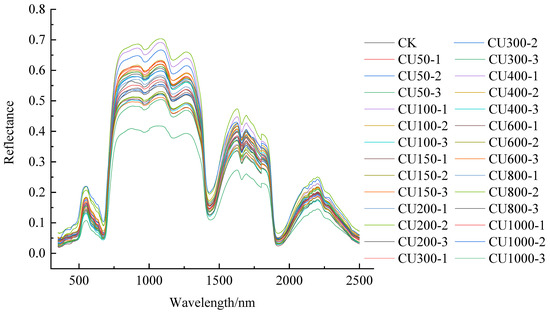
Figure 2.
The original spectral curve of the corn leaves under different gradients of copper stress.
The CR and DRS spectral transformations were performed concurrently on the original spectral curves, and the results are shown in Figure 3 and Figure 4, respectively. The peaks and valleys of the curves were more visible after the CR transformation process, as shown in Figure 3. After the DRS transformation process, the spectral characteristics of the vegetation in the curves had disappeared, leaving only the characteristics of the copper elements visible, as shown in Figure 4.
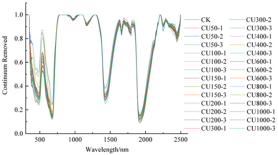
Figure 3.
Continuum removed spectral transformation.
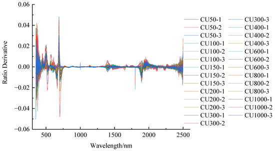
Figure 4.
Derivative of the ratio spectroscopy.
The spectral characteristics of the curves evidently improved after the spectral transformation process, but the spectral curves’ noise effect remained. To remove the noise effect, SVD was applied to the OS, CR, and DRS, where the sum of the first seven singular values of the OS reached 90% of the overall singular values, the sum of the first eleven singular values of the CR reached 90% of the overall singular values, and the sum of the first seventeen singular values of the DRS reached 90% of the overall singular values. As a result, the OS chose the first seven components for reconstruction; CR chose the first eleven components for reconstruction; and DRS chose the first seventeen components for reconstruction. The reconstructed curves are shown in Figure 5. The overall trends of the reconstructed curves with different transformation methods, as well as the spectral curves without SVD treatment, were all consistent, and the original characteristics were preserved, while the noise effects were removed.
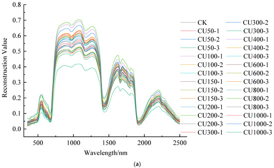
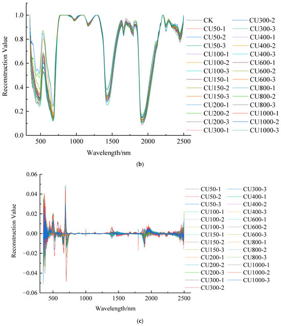
Figure 5.
SVD reconstruction curve. (a) OS; (b) CR; and (c) DRS.
3.2. Extraction of Characteristic Bands
Pearson correlation analysis was performed, band by band, on the spectral training set data of the corn leaves with different levels of copper stress. In the analysis, the measured copper content and the correlation coefficient between each band and copper content was calculated. The bands that passed the p = 0.01 significance test were chosen as the initial selection of the characteristic band. The correlations between each band and copper content before and after SVD treatment were compared and analyzed to demonstrate the effect of the SVD treatment. The comparison results are shown in Figure 6.
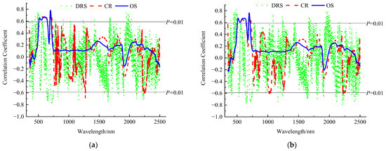
Figure 6.
Comparative analysis of the correlations between the copper content and various bands before and after SVD treatment. (a) Before SVD processing and (b) after SVD processing.
As shown in the figure, after the CR and DRS spectral transformation treatments, the correlation between the corresponding data of each band and copper content increased more clearly than in the OS, and the DRS increased more clearly than the CR. The number of bands passing the p = 0.01 significance test for the three types of data increased significantly after SVD treatment, as shown in Table 2 for the specific data comparison. The DRS transform has the highest number of bands passing the p = 0.01 significance test after the SVD treatment, as shown in the table, with 228 bands passing.
Table 2.
Number of bands passing the p = 0.01 correlation significance test.
The data for the preliminary selected characteristic bands that passed the correlation significance test were subjected to a mutual information analysis of the copper content, and the top 10 bands were chosen as the characteristic bands for model establishment in the order of the MI values from the largest to smallest, as shown in Table 3.
Table 3.
Characteristic bands of the training set extracted by MI.
3.3. Construction of the PLSR Model and Accuracy Evaluation
Based on the OS, CR, and DRS correlation analyses, the PLSR prediction models were built, and the characteristic bands of the training set samples were determined by mutual information, whereby the number of principal components of each model were determined first. Figure 7 depicts the RMSEP and CCR results of the models established by the three transformations of OS, CR, and DRS. It can be seen from the figure that the PLSR prediction models established by using the OS, CR, and DRS had an RMSEP that was close to 0 and where the CCR reached 0.99 when the number of principal components was 4, 2, and 2, respectively.
Figure 7.
The RMSEP and CCR of the three transformation modes. (a) OS; (b) CR; and (c) DRS.
The PLSR prediction model was created according to the chosen master fraction, and the scatter plot of the prediction model effect and accuracy assessment is shown in Figure 8. Figure 8a,b show that the R2 in the training and validation sets of the OS-based prediction model was low, the RMSE was large, and the RPD was less than 1.4, which indicates that the prediction ability of the OS-based prediction model was poor. Figure 8c,d show that the validation set of the prediction model that was established based on CR had a high accuracy, with an R2 of 0.73, an RMSE of 1.19 mg/kg, and an RPD of 1.93. However, the accuracy of the model established by the training set samples was low, and the large gap between the accuracy of the model established by the training set and the validation set samples indicated that the stability of the model was not high. In addition, the RPD was less than 2, thereby indicating a general predictive ability of the model. Figure 8e,f show that the R2 of the DRS prediction model’s training and validation sets was greater than 0.7, the RMSE was small, and the RPD of the training set samples was 2.51, thus indicating that the DRS prediction model has a strong prediction ability and high stability. Overall, the OS-based PLSR prediction model had the lowest predictive power, and it produced the least reliable prediction results. The PLSR prediction model based on CR had a good general prediction ability and achieved better prediction results than OS, but the model’s stability was poor. The PLSR prediction model that is based on DRS outperformed the OS and CR in terms of predictive power and stability.
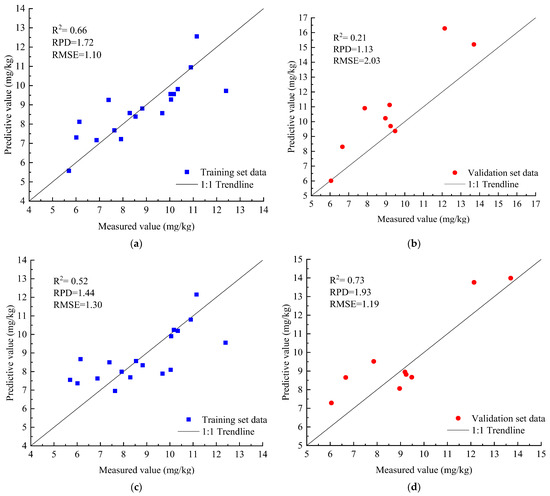
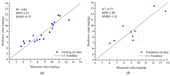
Figure 8.
Scatter diagram and accuracy evaluation of the PLSR model. (a) OS training set; (b) OS validation set; (c) CR training set; (d) CR validation set; (e) DRS training set; and (f) DRS validation set.
3.4. Construction of the XGBoost Model and Accuracy Evaluation
The XGBoost prediction models were built using OS, CR, and DRS correlation analyses, and the training set samples’ characteristic bands were determined by using mutual information. First, the prediction model’s parameters were adjusted, and the XGBoost prediction model’s main parameters were expanded. Grid search was used to determine the optimal parameters of the prediction model that were established based on the OS, CR, and DRS. The training set samples were trained using a nine-fold cross-validation, and the optimal parameters that were obtained are shown in Table 4.
Table 4.
Optimal parameters of the XGBoost prediction model.
The XGBoost prediction model was built using the optimal parameters chosen, and the scatter plot of the prediction model effect and accuracy evaluation are shown in Figure 9. The XGBoost prediction models that were based on OS, CR, and DRS all had high accuracy and strong prediction ability in the training set (as shown in Figure 9), with significant differences in the validation set. Figure 9b shows that the model built using OS had the lowest accuracy with an R2 of 0.45, an RMSE of 1.70, and an RPD of 1.35, thus indicating that the model’s stability was not high, and that the RPD was less than 1.4, thereby indicating that the model had poor predictive ability. Figure 9f shows that the DRS-based model had the highest accuracy, with an R2 of 0.86, an RMSE of 0.86, and an RPD of 2.66, a high model stability, an RPD greater than 2, and a strong predictive ability. In comparison to PLSR, the prediction model based on XGBoost had higher accuracy and prediction ability.
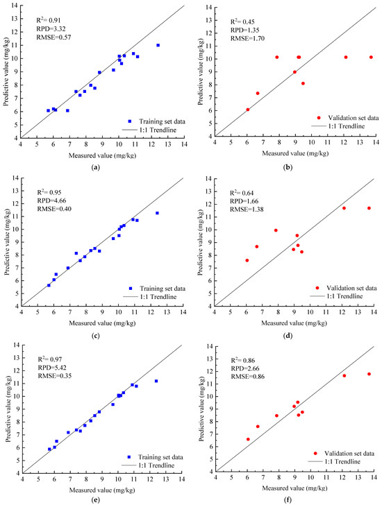
Figure 9.
Scatter diagram and an accuracy evaluation of the XGBoost model. (a) OS training set; (b) OS validation set; (c) CR training set; (d) CR validation set; (e) DRS training set; and (f) DRS validation set.
3.5. Robustness Test of the Model
The visible–near infrared spectral data of the field-grown corn leaves near a mining area in Baoding, Hebei Province, China, were chosen for analysis in order to test the robustness of the two models. In September 2021, fourteen sets of corn leaf samples were collected from different locations near the mining area, and the distribution map of the sampling points is shown in Figure 10.
Figure 10.
Sampling point distribution map.
Healthy corn plants were carefully selected in close proximity to each sampling point, and it was ensured that they were unaffected by pests or diseases. Stainless steel scissors were used to meticulously remove the corn leaves along the stem. The collected corn leaves were preserved in their original condition and securely placed in labeled bags at designated locations. To prevent any cross-contamination with subsequent samples, the scissors were thoroughly cleaned. Three sets of corn leaves were collected from each sampling point. Subsequently, the collected corn leaves were transported to the laboratory. Upon arrival, the leaves were rinsed with deionized distilled water to eliminate any significant contamination that could result from soil or fertilizer spraying. Subsequently, the leaves were air-dried in a natural cool environment until reaching a constant weight. Finally, the indoor spectral data of the corn leaves were meticulously collected, whereby it was ensured that the collection environment and process were consistent with the procedures employed in the previous experiment. The SVC HR-1024I model spectrometer was chosen as the measurement instrument. The sampling interval between the SVC spectrometer and the ASD spectrometer was not consistent; as such, the collected spectral data were first resampled to make the number of bands in the SVC spectrometer consistent with the number of bands in the ASD spectrometer. The collected corn leaves, which were utilized for spectral data analysis, underwent a series of preparatory procedures including cleaning, drying, crushing, and microwave digestion. The determination of copper content in the corn leaves was carried out using an inductively coupled plasma emission spectrometer (ICP-OES), and the corresponding results are presented in Table 5. Upon comparing the data in Table 5 with those in Table 1, it becomes evident that the copper content in the corn leaves near the mining area exhibited a significantly elevated level. This observation strongly suggests that the corn plants in close proximity to the mining site experienced stress due to the presence of high levels of copper, i.e., a heavy metal.
Table 5.
Copper content in the corn leaves near the mining area.
The spectral data collected were processed with the CK group of leaves’ spectral data for the DRS and SVD, and the selected characteristic bands were consistent with those in Table 3. Table 6 displays the accuracy ratings of the prediction models built using PLSR and XGBoost. The table shows that the PLSR-based prediction model had very low accuracy, a negative R2, a large RMSE, an RPD less than 1.4, and poor prediction ability. The XGBoost-based prediction model had an R2 of 0.51, a small RMSE, and an RPD greater than 1.4, thus indicating average prediction ability. This demonstrates that the XGBoost model was more robust than the PLSR model. The accuracy of the prediction model established by field data was low when compared to the model that was established by indoor experiments. However, the prediction model established based on XGBoost also had some prediction ability, thus laying the groundwork for the rapid detection of heavy metal copper in field crops.
Table 6.
Accuracy evaluation of the prediction model.
4. Discussion
In previous studies, hyperspectral technology has been demonstrated to offer several advantages over traditional chemical analysis methods for estimating heavy metal content in crops [31]. Firstly, hyperspectral technology provides comprehensive spectral information, including absorption, reflection, and scattering. These spectral characteristics can capture the variations in the spectral patterns caused by the copper content in leaves, thus enabling the accurate quantification of copper content [32]. Secondly, hyperspectral technology is nondestructive and allows measurements to be taken without causing damage to the leaves. This eliminates the need for sample destruction and reduces waste [33]. Additionally, hyperspectral technology offers high spatiotemporal resolution, thereby allowing for the rapid scanning and monitoring of large-scale corn fields [34].
This study aimed to estimate copper content accurately by collecting the hyperspectral data of corn leaves under different gradients of copper stress, as well as by utilizing the DRS–XGBoost inversion model. The model was successfully applied to farmland near a mining area, thereby yielding satisfactory results. These findings have significant implications for agricultural management and soil pollution monitoring. This research revealed that copper, as a heavy metal, impacts various aspects of corn leaves, including chlorophyll content, greenness, leaf structure, and water content, which can be reflected in the spectral curves of corn leaves. In particular, the spectral range of 780–1300 nm, which corresponds to the internal structure of corn leaves, exhibited the most significant differences. This finding aligns with the research conducted by Zhu et al. [35]. Given the small spectral interval and large data volume of the hyperspectral data, there may be data redundancy. Appropriate spectral transformation techniques can effectively eliminate noise and enhance spectral features [36]. In this study, the SVD, CR, and DRS methods all demonstrated favorable outcomes by preserving the original characteristics and important information of the spectral curve while improving the correlation with copper content. Notably, the SVD–DRS approach exhibited the most pronounced effect. PLSR, a traditional statistical method [37], and XGBoost, a powerful machine learning method [38], were both employed in this study as regression analysis techniques that are widely used in the field. A comparative analysis of the PLSR and XGBoost prediction models revealed that the XGBoost model achieved higher prediction accuracy and better robustness, which is consistent with the research findings of Lin et al. [39].
There are several challenges and limitations associated with the study of hyperspectral inversion for estimating the copper content in corn leaves. Firstly, the choice of inversion models significantly affects the accuracy and stability of the results. Different inversion models have varying assumptions and limitations in processing and analyzing spectral data. Therefore, it is crucial to consider factors such as accuracy, robustness, and computational efficiency when selecting an inversion model. Secondly, the influence of external factors on spectral data should also be taken into account. Factors such as lighting conditions, leaf physiological status, and soil moisture levels can impact spectral data, thereby subsequently affecting the accuracy of the inversion results. Thirdly, the availability and quality of reference data for model calibration and validation pose challenges. Accurate and representative reference data are essential for training and evaluating the inversion models. However, obtaining such data can be time-consuming and resource-intensive. Additionally, the generalizability of the inversion models should be considered. The performance of the models may vary when applied to different regions or when under different environmental conditions. Therefore, it is necessary to validate the models across various locations and conditions to assess their reliability and applicability. In conclusion, this study showcases the potential of hyperspectral inversion as a method for accurately estimating copper content in corn leaves. Despite the existing challenges and limitations, this technique offers a rapid, nondestructive, and quantitative approach that holds promise for agricultural management and environmental monitoring. Further research endeavors can focus on refining inversion algorithms, enhancing estimation accuracy, and investigating the potential applications of hyperspectral technology in diverse crop and environmental domains.
5. Conclusions
Based on the visible–NIR spectral data of corn leaves undergoing different gradients of heavy metal copper stress, the respective spectra were classified as OS, CR, and DRS. The spectra were denoised using SVD, and the characteristic bands were selected by CA and MI to build a prediction model of the copper content in corn leaves based on PLSR and XGBoost. The model’s robustness was tested using visible–near infrared spectral data from field-grown corn leaves near a mining site. The findings are as follows:
(1) Spectral transformation processing can improve the correlation between spectral data and copper content, with DRS having a more pronounced effect than CR. (2) SVD effectively removed the influence of noise in spectral data and improved the correlation between spectral data and copper content, while the DRS had a higher number of bands passing the p = 0.01 significance test. (3) The accuracy of the PLSR and XGBoost prediction models based on spectral transform was higher than the original data, whereby the XGBoost model that is based on DRS had the highest accuracy in the validation set, with an R2 of 0.86, an RMSE of 0.86 mg/kg, and an RPD of 2.66. (4) The robustness of the DRS-based XGBoost model outperformed that of the PLSR model.
The research method presented in this article offers novel insights and solutions for the efficient detection of copper content, a heavy metal, in crops. Furthermore, it serves as a valuable reference for predicting the content of other heavy metals in crops. This study establishes an XGBoost prediction model that is based on DRS, which enables the rapid and accurate prediction of copper content in crops. This achievement lays a solid foundation for addressing areas affected by heavy metal pollution.
Author Contributions
Conceptualization, B.W., K.Y. and Y.L.; methodology, B.W., K.Y. and Y.L.; software, B.W.; validation, B.W.; formal analysis, B.W.; investigation, B.W.; data curation, B.W. and K.Y.; writing—original draft preparation, B.W.; writing—review and editing, B.W., Y.L. and J.H.; visualization, B.W.; supervision, K.Y. and J.H.; funding acquisition, K.Y. All authors have read and agreed to the published version of the manuscript.
Funding
This research was funded by the Science and Technology Fundamental Resources Investigation Program (2022FY101905), the National Natural Science Foundation of China (41971401), and the China University of Mining and Technology (Beijing) Doctoral Student Top Innovative Talent Cultivation Fund Project (BBJ2023017).
Institutional Review Board Statement
Not applicable.
Informed Consent Statement
Not applicable.
Data Availability Statement
Data are contained within the article.
Conflicts of Interest
The authors declare no conflict of interest.
References
- Liu, S.; Peng, B.; Li, J. Ecological Risk Evaluation and Source Identification of Heavy Metal Pollution in Urban Village Soil Based on XRF Technique. Sustainability 2022, 14, 5030. [Google Scholar] [CrossRef]
- Wu, Y.; Li, X.; Yu, L.; Wang, T.; Wang, J.; Liu, T. Review of soil heavy metal pollution in China: Spatial distribution, primary sources, and remediation alternatives. Resour. Conserv. Recycl. 2022, 181, 14. [Google Scholar] [CrossRef]
- Chakraborty, S.; Man, T.; Paulette, L.; Deb, S.; Li, B.; Weindorf, D.; Frazier, M. Rapid assessment of smelter/mining soil contamination via portable X-ray fluorescence spectrometry and indicator kriging. Geoderma 2017, 306, 108–119. [Google Scholar] [CrossRef]
- Chakraborty, S.; Weindorf, D.C.; Deb, S.; Li, B.; Paul, S.; Choudhury, A.; Ray, D.P. Rapid assessment of regional soil arsenic pollution risk via diffuse reflectance spectroscopy. Geoderma 2017, 289, 72–81. [Google Scholar] [CrossRef]
- Fu, P. Study on the Difference and Inversion of Soil Copper and Lead Concentration in Frequency Domain Spectrum; China University of Mining and Technology: Beijing, China, 2019. [Google Scholar]
- Gujre, N.; Mitra, S.; Soni, A.; Agnihotri, R.; Rangan, L.; Rene, E.R.; Sharma, M.P. Speciation, contamination, ecological and human health risks assessment of heavy metals in soils dumped with municipal solid wastes. Chemosphere 2020, 262, 128013. [Google Scholar] [CrossRef]
- Bawa, U. Heavy metals concentration in food crops irrigated with pesticides and their associated human health risks in Paki, Kaduna State, Nigeria. Cogent Food Agric. 2023, 9, 24. [Google Scholar] [CrossRef]
- Food and Agriculture Organization of the United Nations. World Food and Agriculture; Food and Agriculture Organization: Rome, Italy, 2012. [Google Scholar]
- Li, Y.; Yang, K.; Rong, K.; Zhang, C.; Gao, P. Spectral characteristics and monitoring of maize under heavy metal copper stress. Spectrosc. Spectr. Anal. 2019, 39, 2823–2828. [Google Scholar]
- Dai, W. Effects of Heavy Metals on Growth and Physiological and Biochemical Characteristics of Maize; Gansu Agricultural University: Lanzhou, China, 2017. [Google Scholar]
- Song, R.; Feng, Y.; Cheng, W.; Wang, X. Advance in Hyperspectral Images Change Detection. Spectrosc. Spectr. Anal. 2023, 43, 2354–2362. [Google Scholar] [CrossRef]
- Gu, Y.; Liu, T.; Gao, G.; Ren, G.; Ma, Y.; Chanussot, J.; Jia, X. Multimodal hyperspectral remote sensing: An overview and perspective. Sci. China Inf. Sci. 2021, 64, 24. [Google Scholar] [CrossRef]
- Bioucas-Dias, J.M.; Plaza, A.; Camps-Valls, G.; Scheunders, P.; Nasrabadi, N.; Chanussot, J. Hyperspectral remote sensing data analysis and future challenges. IEEE Geosci. Remote Sens. Mag. 2013, 1, 6–36. [Google Scholar] [CrossRef]
- Yan, C.S.; Chen, Y.W.; Yang, H.M.; Ahokas, E. Optical spectrum analyzers and typical applications in astronomy and remote sensing. Rev. Sci. Instrum. 2023, 94, 30. [Google Scholar] [CrossRef] [PubMed]
- Pearlshtien, D.H.; Pignatti, S.; Greisman-Ran, U.; Ben-Dor, E. PRISMA sensor evaluation: A case study of mineral mapping performance over Makhtesh Ramon, Israel. Int. J. Remote Sens. 2021, 42, 5882–5914. [Google Scholar] [CrossRef]
- Zaib, M.; Sarfaraz, A.; Akhtar, N.; Shahzadi, T. Sensitive determination of Cu (II) ions using different doped carbon dot and silver nanocomposites: Comparative study. Int. J. Environ. Sci. Technol. 2022, 19, 9861–9872. [Google Scholar] [CrossRef]
- Zhang, Q.; Zhang, H.; Zhang, H.; Wang, X.S.; Liu, W.K. Hybrid Inversion Model of Heavy Metals with Hyperspectral Reflectance in Cultivated Soils of Main Grain Producing Areas. Trans. Chin. Soc. Agric. Mach. 2017, 48, 148–155. [Google Scholar]
- Zhang, Z.; Liu, M.; Liu, X.; Zhou, G. A New Vegetation Index Based on Multitemporal Sentinel-2 Images for Discriminating Heavy Metal Stress Levels in Rice. Sensors 2018, 18, 2172. [Google Scholar] [CrossRef] [PubMed]
- Mirzaei, M.; Verrelst, J.; Marofi, S.; Abbasi, M.; Azadi, H. Eco-Friendly Estimation of Heavy Metal Contents in Grapevine Foliage Using In-Field Hyperspectral Data and Multivariate Analysis. Remote Sens. 2019, 11, 2731. [Google Scholar] [CrossRef]
- Zhong, L.; Chu, X.; Qian, J.; Li, J.; Sun, Z. Multi-Scale Stereoscopic Hyperspectral Remote Sensing Estimation of Heavy Metal Contamination in Wheat Soil over a Large Area of Farmland. Agronomy 2023, 13, 2396. [Google Scholar] [CrossRef]
- Liu, H.; Niu, T.; Yu, Q.; Su, K.; Yang, L. Inversion and Estimation of Heavy Metal Element Content in Peach Forest Soil in Pinggu District of Beijing. Spectrosc. Spectr. Anal. 2022, 42, 3552–3558. [Google Scholar] [CrossRef]
- Yang, H.; Du, J. Classification of desert steppe species based on unmanned aerial vehicle hyperspectral remote sensing and continuum removal vegetation indices. Optik 2021, 247, 167877. [Google Scholar] [CrossRef]
- Chen, C.; Jiang, Q.; Zhang, Z.; Shi, P.; Xu, Y.; Liu, B.; Xi, J.; Chang, S. Hyperspectral Inversion of Petroleum Hydrocarbon Contents in Soil Based on Continuum Removal and Wavelet Packet Decomposition. Sustainability 2020, 12, 4218. [Google Scholar] [CrossRef]
- Zhao, H.; Zhang, L.; Cen, Y.; Wu, T.; Wang, J. Analysis of strong linear band characteristics based on ratio derivative spectroscopy. J. Infrared Millim. Waves 2013, 32, 563–568. [Google Scholar] [CrossRef]
- Wang, J.; Cao, L.; Xu, G.; Feng, X.; Wu, B. Study on hyperspectral detection method of sodium sulfate corrosion products in concrete. Spectrosc. Spectr. Anal. 2019, 39, 1724–1730. [Google Scholar]
- Chen, T.Q.; Guestrin, C. XGBoost: A scalable tree boosting system. In Proceedings of the 22nd ACM SIGKDD International Conference on Knowledge Discovery and Data Mining, San Francisco, CA, USA, 13–17 August 2016; ACM: New York, NY, USA, 2016; pp. 785–794. [Google Scholar]
- Tian, Y.; Huang, H.; Zhou, G.; Zhang, Q.; Tao, J.; Zhang, Y.; Lin, J. Aboveground mangrove biomass estimation in Beibu Gulf using machine learning and UAV remote sensing. Sci. Total Environ. 2021, 781, 146816. [Google Scholar] [CrossRef]
- Hong, Y.; Chen, Y.; Zhang, Y.; Liu, Y.; Liu, Y.; Yu, L.; Liu, Y.; Cheng, H. Transferability of Vis-NIR models for Soil Organic Carbon Estimation between Two Study Areas by using Spiking. Soil Sci. Soc. Am. J. 2018, 82, 1231–1242. [Google Scholar] [CrossRef]
- Liu, Y.; Xu, H.; Sun, X.; Jiang, X.; Rao, Y. Study on general model for online detection of sugar content in different varieties of apple by near infrared spectroscopy. Spectrosc. Spectr. Anal. 2020, 40, 922–928. [Google Scholar]
- Summers, D.; Lewis, M.; Ostendorf, B.; Chittleborough, D. Visible near-infrared reflectance spectroscopy as a predictive indicator of soil properties. Ecol. Indic. 2011, 11, 123–131. [Google Scholar] [CrossRef]
- Zhang, S.; Fei, T.; Chen, Y.; Hong, Y. Estimating cadmium-lead concentrations in rice blades through fractional order derivatives of foliar spectra. Biosyst. Eng. 2022, 219, 177–188. [Google Scholar] [CrossRef]
- Zhao, H.; Cui, B.; Jia, G.; Gan, F. The influence analysis of reflectance anisotropic of canopy on the prediction accuracy of Cu stress based on laboratory multi-directional measurement. In Proceedings of the International Conference on Optical Instruments and Technology—Optoelectronic Imaging/Spectroscopy and Signal Processing Technology, Beijing, China, 26–28 October 2019; Spie-Int Soc Optical Engineering: Bellingham, WA, USA, 2020. [Google Scholar]
- Saha, D.; Manickavasagan, A. Machine learning techniques for analysis of hyperspectral images to determine quality of food products: A review. Curr. Res. Food Sci. 2021, 4, 28–44. [Google Scholar] [CrossRef]
- Li, C.; Cui, Y.; Ma, C.; Niu, Q.; Li, J. Hyperspectral inversion of maize biomass coupled with plant height data. Crop Sci. 2021, 61, 2067–2079. [Google Scholar] [CrossRef]
- Zhu, Y.; Qu, Y.; Liu, S.; Cheng, S. Spectral response of wheat and lettuce to copper pollution. J. Remote Sens. 2014, 18, 335–352. [Google Scholar]
- Shen, L.; Gao, M.; Yan, J.; Li, Z.-L.; Leng, P.; Yang, Q.; Duan, S.-B. Hyperspectral Estimation of Soil Organic Matter Content using Different Spectral Preprocessing Techniques and PLSR Method. Remote Sens. 2020, 12, 1206. [Google Scholar] [CrossRef]
- Wang, Q.; Jin, J. Leaf transpiration of drought tolerant plant can be captured by hyperspectral reflectance using PLSR analysis. iForest—Biogeosci. For. 2016, 9, 30–37. [Google Scholar] [CrossRef]
- Loggenberg, K.; Strever, A.; Greyling, B.; Poona, N. Modelling Water Stress in a Shiraz Vineyard Using Hyperspectral Imaging and Machine Learning. Remote Sens. 2018, 10, 202. [Google Scholar] [CrossRef]
- Lin, N.; Fu, J.; Jiang, R.; Li, G.; Yang, Q. Lithological Classification by Hyperspectral Images Based on a Two-Layer XGBoost Model, Combined with a Greedy Algorithm. Remote Sens. 2023, 15, 3764. [Google Scholar] [CrossRef]
Disclaimer/Publisher’s Note: The statements, opinions and data contained in all publications are solely those of the individual author(s) and contributor(s) and not of MDPI and/or the editor(s). MDPI and/or the editor(s) disclaim responsibility for any injury to people or property resulting from any ideas, methods, instructions or products referred to in the content. |
© 2023 by the authors. Licensee MDPI, Basel, Switzerland. This article is an open access article distributed under the terms and conditions of the Creative Commons Attribution (CC BY) license (https://creativecommons.org/licenses/by/4.0/).