Prediction of CO₂ Emissions Related to Energy Consumption for Rural Governance

Abstract

In the context of rural revitalization, many industries have begun to shift towards rural areas. Industrial agglomeration not only brings economic growth to rural areas, but also increases local carbon emissions. This is particularly evident in some industrialized rural areas with high energy consumption. To accurately implement rural environmental governance, this study selected population, energy consumption, coal proportion, urbanization rate, and other factors as the influencing factors of carbon emissions. The grey correlation analysis method was used to obtain the correlation coefficient of the influencing factors. Then, the relationship between carbon emissions and economic growth, energy consumption, and other influencing factors was analyzed from multiple perspectives. In addition, this study constructed an energy consumption carbon emission prediction model based on deep learning networks, aiming to provide reference data for rural greenhouse gas emission reduction. These results confirmed that the correlation coefficients of the influencing factors of carbon emissions were all higher than 0.6, indicating that their carbon emissions were highly correlated. These test results on the dataset confirm that the RMSE values of the proposed model are all around 0.89, indicating its good prediction accuracy. Therefore, the proposed carbon emission prediction model can provide scientific and reasonable reference data for rural air governance.

1. Introduction

China is a major energy consumption (EC) country, with coal, oil, and natural gas as the main sources of fossil fuel consumption, making it a carbon emission (CE) country. The rapid urbanization process has led to a sharp increase in the number of urban residents, and EC has also been continuously increasing [1]. With urbanization, the construction land in rural areas is also increasing day by day. Over the past thirty years, the development mode of “high pollution, high EC, and high emissions” has led to a great waste of land resources, and has also strengthened the role of “carbon source” and weakened the role of “carbon sink” [2]. Ultimately, this has led to a significant increase in CE in urban and rural areas of China, resulting in rapid degradation of the ecological and living environment in both urban and rural areas. This has a significant impact on the socio-economic and environmental sustainability of urban and rural areas [3,4]. On the one hand, the development of rural economy has greatly improved the lives of villagers. The per capita household necessities of farmers are increasing, and their living habits are also becoming closer to those of cities and towns. On the other hand, this has also led to an increasing level of EC in rural areas, as well as an increasing amount of exhaust and waste emissions from villagers’ production and daily life. The EC of rural residents has gradually shown the characteristics of “high carbonization” [5]. Especially for heavy industrial areas, industrial transfer has become a condition for rapid development of rural economy and a factor affecting high emissions in rural areas. Industry is a very important material production industry, playing a crucial role in the entire national economic system [6]. At present, there is a huge EC in China’s industrial development, which is parallel to the rapid development of the Chinese economy. After the reform and opening up, rural industries in China have developed rapidly, presenting a unique development trend in East Asia. This trend constitutes China’s unique mode of industrialization development, enabling rural areas in China to find a practical development path in the process of industrialization [7,8]. After the 21st century, rural industry has become an important economic growth point in the national economy. By 2005, the added value of rural enterprises had reached CNY 400 billion, with an average annual growth rate exceeding 10%. The industrial added value in rural areas accounts for 44% of the total national income, while employment in rural areas accounts for 43% of the country’s non-agricultural employment, and 34% of its exports are derived from industries in rural areas [9]. However, in promoting the development of rural industry, it has also had adverse effects on the ecological environment, farmers’ lives, agricultural production, EC, etc. The sustainable development of rural industries refers to the emphasis on the effective utilization and conservation of resources, aiming to reduce dependence on and loss of natural resources in the process of economic development by promoting sustainable production and consumption methods, adopting efficient resource utilization technologies and circular economy models, achieving coordinated economic growth and environmental protection, and promoting sustainable development. In rural environmental governance, measures should be taken to reduce waste in agricultural production processes and improve the efficiency of agricultural resource utilization. Therefore, on the premise of ensuring the efficient development of rural industries, reducing the pollution caused by industries, thereby saving energy and reducing emissions, is a key issue that needs to be addressed in the sustainable development of rural industries. Given this, this study will use grey relation analysis (GRA) to measure the degree of correlation between CE factors affecting industrialized rural areas. And this study takes into account the collaboration of spatiotemporal features and constructs Spatial Temporal Graph Convolutional Networks (ST-GCN) for rural CE prediction.

The full text mainly includes the following four parts. Firstly, there is a literature review on EC and CE prediction models. The second part is an analysis of influencing factors and the construction of quantitative prediction models for high-EC rural areas. The third part is an analysis of the correlation degree of carbon driving factors and the utility of prediction models. Finally, there is a summary on the GRA and prediction models proposed by this research.

2. Related Works

In order to achieve modern development, traditional rural areas have transformed from a small-scale peasant economy to an industrial economy, which has enabled rural revitalization, but has also brought about a huge environmental crisis. In order to achieve sustainable social and economic development, determining how to carry out rural governance has become crucial. The problem that needs to be addressed in this study is how to construct a measurement method for carbon emissions in industrialized rural areas and their influencing factors, and how to solve and predict carbon emissions based on deep learning models. In rural governance research, Brown D explores how rural settlements are urbanized and how rural governance is transformed in this process. The article proposes a comparative agenda aimed at exploring and comparing the institutional changes that have occurred in the ‘transitional space’, the complexity of governance brought about by these changes, and the consequences of establishing urban planning systems in rural settlements in history [10]. Researchers such as Bhuvana M have measured the satisfaction of rural residents by analyzing the service quality of e-government public service centers. The causal relationship was tested through structural formula modeling. Research has found that trust, availability, and information quality are the main factors in evaluating the service quality of public service centers using e-government services [11]. Yaacoub E et al. believe that accessing the internet will provide people living in rural or impoverished areas with the possibility of making progress in education, health, environment, and business levels. Therefore, the main limitation in providing connectivity between rural and impoverished areas is the cost of return deployment. In addition, they conducted an analysis of the energy demand and cost-effectiveness of the studied technology [12]. Yaacoub E conducted research on IoT connectivity in rural areas, discussing intelligent wireless resource management and network planning technologies for IoT access/front-end networks. These results confirm the good performance of the proposed method in scheduling IoT devices [13].

In terms of EC, scholars such as Kirikkaleli D explore the impact of renewable EC and public–private partnership energy investment on India’s CO₂ emissions while controlling technological innovation and economic growth. These results confirm a long-term co-integration relationship between consumption-based CE quantity and its possible determinants [14]. Dong K et al. investigated the emission–growth–renewable energy relationship of a global panel consisting of 120 countries and four income-based subpanels from 1995 to 2015. Research has shown significant differences in the impact of renewable EC on CO₂ emissions for various income-based sub panels [15]. Murad M W et al. investigate the dynamic relationship between technological innovation, EC, energy prices, and economic growth in Denmark from 1970 to 2012, using multivariate settings to test time series data. This analysis uses the autoregressive distribution lag (ARDL) method for co-integration to examine the short-term and long-term dynamics between variables [16].

Many scholars have conducted rich and colorful research on CE prediction. Wei Z et al. used the Tapio decoupling model to explore the relationship between CE and the economy in Henan Province. They used the STIRPAT extended model and ridge regression to study the influencing factors of CE in Henan Province, and obtained the CE prediction formula. These results confirm that the energy intensity effect and energy structure effect can promote the optimization of the relationship between Henan Province’s economy and CE. The energy structure and CE intensity have a significant negative impact on CE, while the industrial structure has a significant positive impact on CE [17]. Liu Y and other scholars propose an EC prediction method based on the efficiency of global data center transportation and electricity usage to predict and analyze the future EC and CE of global data centers. This study provides support for global EC forecasting and guides the layout of future global data centers from an EC perspective. In addition, it provides support for the feasibility of integrating energy and information networks under the concept of global energy interconnection [18]. Adame M F et al. integrated a comprehensive global dataset of carbon storage, mangrove distribution, deforestation rates, and land use change drivers into the mangrove CE prediction model. It predicts the “normal” emissions and soil carbon sequestration potential of mangrove loss rates. These results confirm the areas where policy action is needed to address emissions caused by mangrove loss, as well as the driving factors that can be found to prevent these emissions [19]. Yu Y et al. established an extended population, affluence, and technology regression stochastic impact model to study the impact of technological innovation on CO₂ emissions. These results confirm that with the introduction of appropriate technological innovation policies by the government during the “New Normal” period, China will make new progress in CO₂ emission reduction in the future [20]. Ran Q et al. used random forest technology to filter out factors affecting industrial CE in order to slow down global warming and promote low-carbon economic development. These statistical results confirm that the predicted values of industrial CO₂ emissions are surprisingly close to the actual values. By 2030, the industrial sector’s CE will reach its highest level [21]. Lv T et al. used regression population, wealth, and technology random impact models to understand the complex relationship and impact mechanism between urbanization and CE. They analyzed the impact and differential effects of urbanization and population on CE in the ecological civilization demonstration zone of Jiangxi Province. In addition, scenario analysis was used to define nine development scenarios and predict the future CE of Jiangxi Province. These results confirm that from the perspective of spatiotemporal pattern, the changes in CE in Jiangxi Province are uneven. The CE in the peripheral area has significantly increased [22]. Jin I’s prediction model based on Kaya’s identity was used to simulate the CE path before the target year. These results confirm the need to design a climate policy that improves energy and carbon intensity by accelerating technological advancements in climate [23].

In summary, the research direction of rural governance is mainly based on statistical methods for data analysis, with less reliance on intelligent prediction models. In CE research, scenario analysis and random impact models are often used. But there are few studies that combine the two to study the impact and prediction of rural CE. In view of this, this study will construct a CE influencing factor analysis and prediction model based on GRA and ST-GCN to provide a data reference for rural low-carbon governance.

3. Construction of CE Prediction Model for Air Governance in Industrialized Rural Areas

Obtaining accurate CE information is crucial for decomposing the driving factors in CE. This study introduces how to calculate CO₂ emissions from industrial and rural areas, and conducts research on CO₂ emissions and their influencing factors. GRA is used to determine the degree of correlation between various influencing factors and CO₂ emissions to construct subsequent regional CO₂ prediction models.

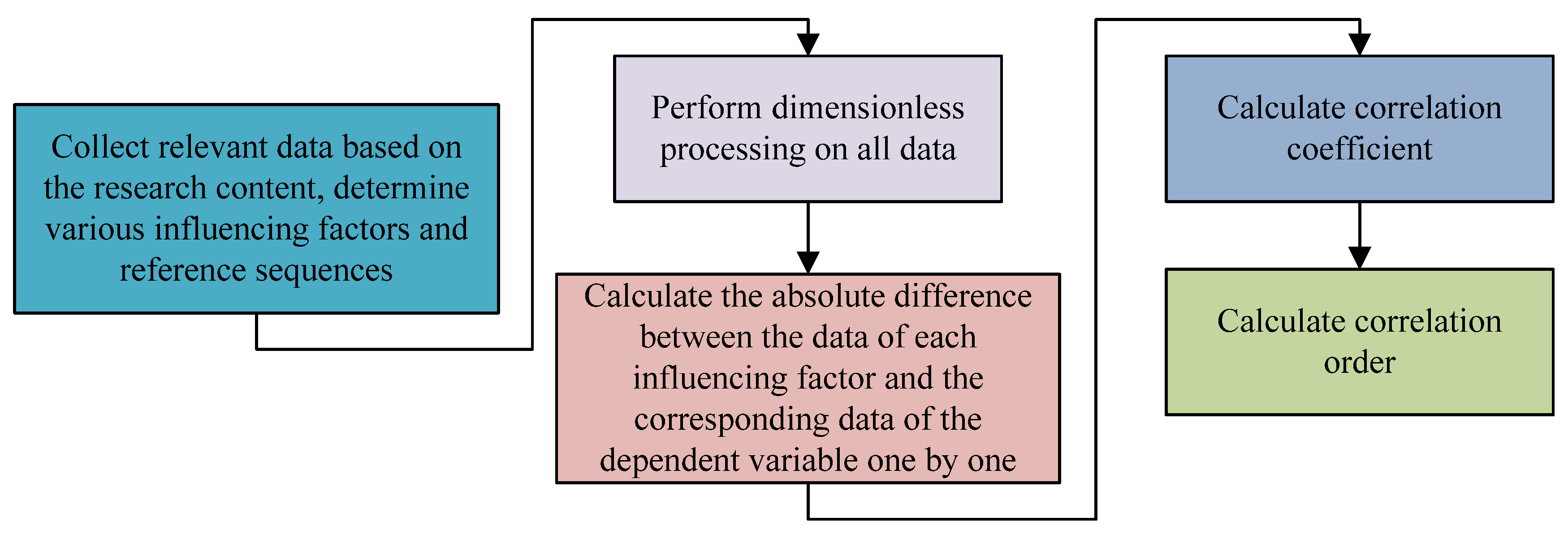
3.1. Calculation of CE in Industrialized Rural Areas and Analysis of Influencing Factors

To ensure the accuracy of various EC calculations, it is necessary to obtain correct EC quantity data and obtain the correlation coefficients of various ECs to provide necessary data support for accurate estimation of energy consumption CE quantity. Previously, most calculations on CE were based on data from three minerals, namely coal, oil, and natural gas [24,25]. Their advantages are also obvious, that is, the data are easy to obtain and the calculation is relatively easy. However, these studies overlook the fact that the proportions of various types of energy and the CE factors generated are different, resulting in computational errors [26]. Therefore, increasing the types of energy involved in the calculation and then calculating the CE quantity will result in more accurate CE calculation results. In terms of obtaining CE factors, the CO₂ ratio of the Climate Change Panel is used by most scientists to calculate CO₂ emissions. Therefore, the CO₂ index in the guidelines issued by the Climate Change Panel can be used to calculate the CO₂ emissions of the study area [27]. Formula (1) is the calculation for CO₂ generated after energy use.

$$C_E={\displaystyle \sum _{i=1}^n{E}_i\times S_i\times \alpha }$$

(1)

In Formula (1), C_E represents the CE quantity, expressed in 10,000 tons. E_i represents the energy consumption of the i-th type in billions of cubic meters [28]. S_i represents the CE coefficient corresponding to the i-th energy source in tons of fuel. α represents the conversion factor between carbon and CO₂, dimensionless, with a value of 44/12. Formula (2) is the CE coefficient.

$$\left\{\begin{array}{l}H{V}_i=C{F}_i\times 29.307\times {10}^3\\ C_i=N_i\times H{V}_i\times \beta \end{array}\right..$$

(2)

In Formula (2), HV_i represents the heat of the i-th energy source in megajoules. HV_i represents the coefficient of converting standard coal for the i-th energy source, dimensionless. C_i represents the CE coefficient of the i-th energy source in tons of fuel. β represents the conversion coefficient between gram and ton, with a value of 1 × 10⁻⁶ [29,30]. N_i represents the oxidation rate of the fuel, taken as 100% of the ideal state.

Table 1. CE coefficient of main types of energy.

Number	Energy Type	Conversion Coefficient of Standard Coal (kg Standard coal/kg)	CE Coefficient (ton of Carbon/ton)
1	Raw coal	0.71	2.02
2	Washed coal	0.90	2.46
3	Coke	0.97	3.08
4	Crude oil	1.43	3.09
5	Gasoline	1.47	2.99
6	Kerosene	1.47	3.10
7	Diesel oil	1.46	3.16
8	Fuel oil	1.43	3.24
9	Liquefied petroleum gas	1.71	3.17
10	Natural gas	1.33	21.87

shows the CE coefficients of the main types of energy. The carbon emission coefficient shown in Table 1 refers to the amount of carbon emissions per unit of energy generated during the combustion or use of each type of energy. In the process of carbon emission accounting, carbon emission coefficients will be used to calculate the emissions of each stage. Carbon accounting through carbon emission coefficients can directly quantify carbon emission data, which is crucial for the operation of the carbon trading market. We converted the physical statistics of various energy consumptions into standard statistics, multiplied them by their respective carbon emission coefficients, and added them up to obtain the total carbon emissions.

From Table 1, the energy sources with a CE coefficient higher than 3.0 are coke, crude oil, kerosene, diesel, fuel oil, and liquefied petroleum gas. Only raw coal, washed coal, and natural gas have a CE coefficient lower than 2.5. Due to different influencing factors, CO₂ emissions may also change [31,32]. Quantitatively studying the relationship between various influencing factors and CE, and predicting them based on this, can provide a basis for formulating corresponding carbon reduction policies. Through the organization of research by domestic and foreign researchers on the driving factors of CE volume, factors such as GDP, population size, urbanization rate, EC quantity, and energy types have been discovered, as shown in

Table 2. Influence factors.

Type	Influence Factor	Unit	Definition
1	Population	Ten million	The total number of people living in a certain area or group
2	GDP	CNY trillion	The final result of production activities of all permanent units in a country (or region) within a certain period of time
3	Urbanization rate	%	The proportion of urban population to the total population (including agriculture and non-agriculture)
4	Total industrial output value	CNY trillion	The total amount of products produced within a certain period of time
5	Labor productivity	%	The efficiency of products produced by workers during the reporting period
6	Number of people engaged	Ten thousand people	Total number of people engaged in production and operation
7	EC	100 million tons	The energy resources consumed in the production process that exist in their original form in nature and are not processed or converted

. The increase in population will lead to rapid development of secondary industry, increasing demand for energy use, and ultimately increasing carbon emissions. Population growth leads to greater resource consumption, which in turn increases carbon emissions. The continuous increase in GDP is a key factor leading to an increase in carbon emissions. Energy is an important foundation for improving economic levels and is crucial for the development of national or regional economies. By accelerating the process of industrialization and urbanization to develop the economy, the urban modernization development model will also promote an increase in energy consumption and carbon emissions. The situation of energy consumption can reflect the efficiency of regional energy utilization and the effectiveness of carbon reduction work. The degree of carbon drive varies among different types of energy, so it is also necessary to include it.

Considering that GRA is not limited by the number of samples or the correlation between samples, this study chose it for factor impact analysis. One of the main foundations of GRA is to determine the correlation between points based on the similarity of their overall morphology at each moment. As time passes, the parameters become increasingly close, forming a learning process about the geometric similarity between two or more continuous curves [33,34]. A high similarity indicates a close relationship between them. The foundation of this method is system analysis. Its core is to rank the “factors that affect the development of the system” according to their importance or degree of influence, that is, to rank the correlation between each element and the system. When the correlation between related factors is high, the corresponding factor has a stronger effect. Figure 1 shows the steps of GRA.

According to Figure 1, we firstly collected relevant data based on the research content, determined the influencing factors and reference sequences (dependent variables), and then performed dimensionless processing on all data. Due to the different physical meanings and units of each variable, it is not possible to directly compare and analyze them, or it is difficult to obtain accurate results during analysis. Therefore, when conducting grey correlation analysis, it is generally necessary to perform dimensionless processing on the data. Then, the absolute differences between the data of each influencing factor and the corresponding data of the dependent variable are calculated one by one, and the correlation coefficient between each influencing factor and the dependent variable is calculated in order to measure the correlation between each influencing factor and the dependent variable (reference data), which is called the correlation order [35,36]. Formula (3) is the correlating coefficient ${\varsigma }_i\left(k\right)$ and the correlating degree r_i.

$$\left\{\begin{array}{l}{\varsigma }_i\left(k\right)=\frac{\underset{i,k}{\min }\left|x_o\left(k\right)-x_i\left(k\right)\right|+\rho \underset{i,k}{\max }\left|x_o\left(k\right)-x_i\left(k\right)\right|}{\left|x_o\left(k\right)-x_i\left(k\right)\right|+\rho \underset{i,k}{\max }\left|x_o\left(k\right)-x_i\left(k\right)\right|}\\ r_i=\frac{1}{m}{\displaystyle \sum _{k=1}^m{\varsigma }_i\left(k\right), k=1, 2, \dots , m}\end{array}\right.$$

(3)

In Formula (3), $x_i\left(k\right)$ represents input data. ρ represents the resolution coefficient with a numerical range of 0 to 1. Its low numerical value indicates a small difference between factors, which means it is difficult to distinguish the differences between factors. Usually, ρ is 0.5.

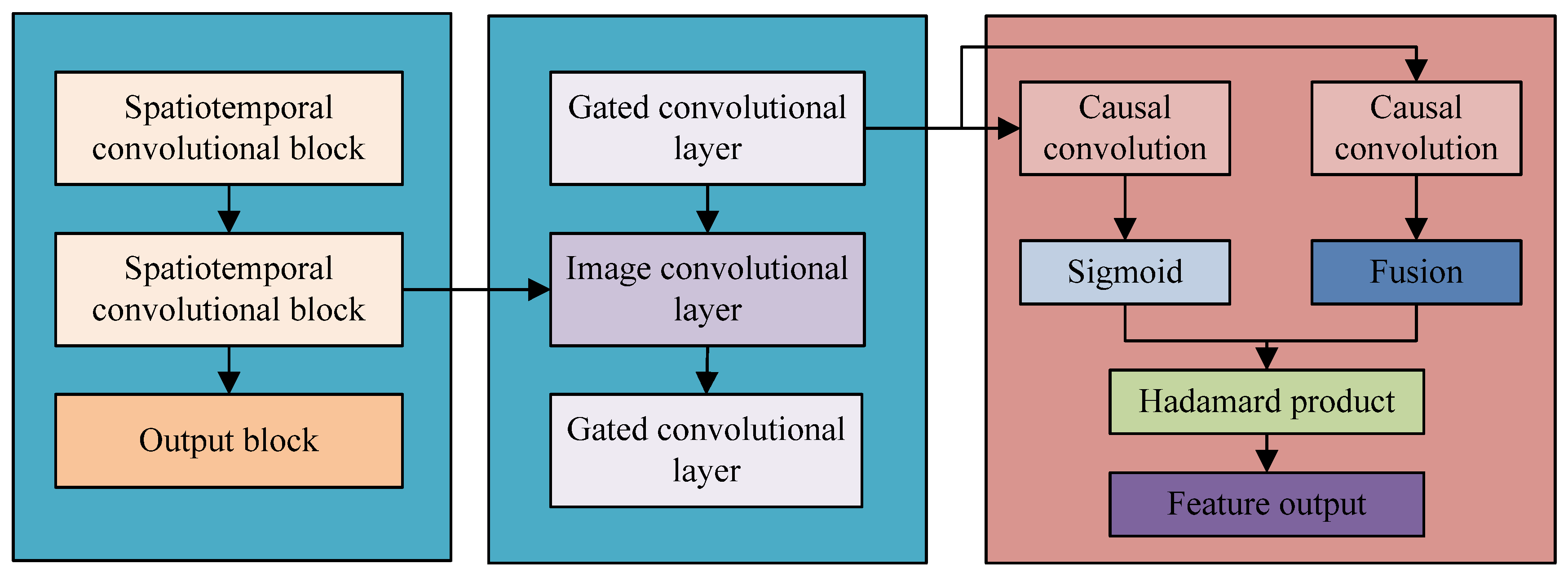
3.2. Construction of CO₂ Emission Prediction Model Based on Deep Learning Network

There are a large number of carbon sources in the industrial production process in rural areas. The spatiotemporal distribution characteristics of its carbon source are complex. Conventional methods for predicting carbon sources and sinks have difficulty effectively analyzing their spatiotemporal characteristics. To address this issue, a new spatiotemporal prediction method based on a graph convolutional network is proposed to improve the applicability of the model in the spatial domain. The prediction problem of CE is to accurately predict the CE data of future networks based on historical data. Based on graph theory, Formula (4) is established to represent the mapping relationship between historical data and future data.

$$\left({\tilde{X}}_{p+1}^1, {\tilde{X}}_{p+2}^1, \dots , {\tilde{X}}_{p+\tau }^1\right)=f\left(\left(X_1, X_2, \dots , X_p\right); G\left(V,E,A\right)\right)$$

(4)

In Formula (4), $\left(X_1, X_2, \dots , X_p\right)$ represents the CE data at ρ time points for a given graph G. By using the mapping function $f\left(\cdot \right)$, historical CE data can be mapped to future CE data $\left({\tilde{X}}_{p+1}^1, {\tilde{X}}_{p+2}^1, \dots , {\tilde{X}}_{p+\tau }^1\right)$. There are certain regional differences in the level of economic development, energy CO₂ emissions, and emission policies among different provinces. Simulating only at the time scale will lead to a lack of in-depth analysis of its spatial characteristics and neglect of its spatiotemporal correlation [37,38]. Therefore, it is vital to analyze the spatiotemporal characteristics and internal connections of CE at the regional scale. Figure 2 is a schematic diagram of graph theory.

The CE network was treated as a graph structure $G=\left(V,E,L\right)$. V represents the collection of provinces and cities in the network, denoted as a node set. E represents the connection relationship between provinces and cities, denoted as an edge set. L represents the Laplace matrix. G represents the topological relationship of a carbon network. Figure 3 shows the topological relationship of the weightless network.

A graph G is composed of N nodes. The adjacency matrix A can be used to describe the interrelationships between these nodes, which can provide a better understanding of the structure of the image [39]. Formula (5) is the neighboring matrix.

$$A_{i,j}=\left\{\begin{array}{l}1,\left(v_i,v_j\right)\in E\\ 0,\left(v_i,v_j\right)\notin E\end{array}\right.$$

(5)

In Formula (5), $\left(v_i,v_j\right)$ represents the combination of nodes. If two nodes are connected, the adjacent matrix value is equal to 1. If there is no connectivity between two nodes, the adjacency matrix of that node is 0. Within a certain period of time, the CE of various rural areas can be described using historical data X and neighboring matrix A [40]. By using spatiotemporal convolution, the interaction between time and space can be displayed, thereby obtaining the predicted results after the i-th node. Figure 4 shows ST-GCN.

ST-GCN is a new type of network based on multiple feature information, consisting of three types of feature sets: spatiotemporal convolution, causal convolution, and graph convolution. These characteristics have their own unique characteristics and can be transformed into each other, forming an efficient integrated network of multiple characteristics. By organically combining two temporal gated convolutional layers with a set of spatial graph convolutional layers, a clear straight cylindrical structure can be obtained. This structure is based on convolutional kernels in the time domain and spatial graph, which can effectively extract complex information. Graph convolution is a neural network used to process graph data, which uses convolution operations to aggregate information between nodes and uses the aggregated information as input, continuously repeating convolution operations until the desired depth is reached. The input of graph convolution is graph data, a convolution operation is performed on the neighbors of each node, and the node is updated with the convolution results. Graph convolution uses a nonlinear activation function to process the convolution results and uses the results as input for the next layer of convolution. Ultimately, graph convolution can transform node states into task-related labels and other outputs. Graph convolution utilizes information from neighboring nodes to extract structural features, while traditional convolutional neural networks are based on image data to better capture and analyze complex models. Formula (6) is time-gated convolution.

$$\Gamma \times \tau X=P\otimes \sigma \left(Q\right)$$

(6)

In Formula (6), Γ represents the region before gated convolution. P and Q represent independent regions’ output after convolution. $\otimes$ represents the Hadamard product. σ represents the sigmoid function. ST-GCN uses a one-dimensional convolution method to solve a nonlinear excitation function. This method takes M as the input order and X as the feature quantity for each node. It is not limited to initial inputs and outputs, and can be repeated multiple times, thus improving the learning results of the model. Formula (7) is spatial graph convolution.

$${\vartheta }_{.g}x=\vartheta \left(L\right)x\approx {\displaystyle \sum _{k=0}^{k-1}{\theta }_k{T}_k\left(\tilde{L}\right)x}$$

(7)

In Formula (7), ${\vartheta }_{.g}$ represents the convolutional kernel. $T_k\left(\tilde{L}\right)$ represents the Chebyshev polynomial, which is used to approximate the characteristics of adjacent nodes at levels 0-k-1 of each node and correct them. This method not only efficiently solves network problems with complex topological structures, but also enhances its learning performance for spatial attributes. When organizing data, it is necessary to normalize it into data within the range of [0, 1]. Currently, in the evaluation parameter indicators of analytical models, data normalization is widely used, with the goal of overcoming the disadvantage of different data units. After normalization, each data point becomes a pure value without units, which is convenient for subsequent comparative analysis of various indicators. Formula (8) is a data normalization method based on maximum standardization.

$$\left\{\begin{array}{l}{x}_i=\frac{x_i-\min x_i}{\max x_i-\min x_i}\\ y_i=\frac{y_i-\min y_i}{\max y_i-\min y_i}\end{array}\right.$$

(8)

By normalizing the data in this way, the raw data are converted into a net value that does not have units and can be used as an index. This value can be applied to compare various variables and improve the performance and generalization ability of the model.

Table 3. Normalized data on factors affecting carbon emissions in industrialized rural areas selected for research.

Region	GDP	Population Size	Urbanization Rate	Energy Consumption	Energy Type
Zhao Wang Zhuang Zhen Lu Er Gang Cun, Laiyang City, Yantai City, Shandong Province	0.0129	0.0187	0.3025	0.0503	0.6467
Pan Shi Dian Zhen Hu Shan Cun, Haiyang City, Yantai City, Shandong Province	0.0163	0.1472	0.4975	0.1056	0.8801
Fang Yuan Jie Dao Mou Jia Cun, Haiyang City, Yantai City, Shandong Province	0.0091	0.0449	0.4827	0.0368	0.9309
Liu Ge Zhuang Zhen Liu Ge Zhuang Cun, Haiyang City, Yantai City, Shandong Province	0.0174	0.1680	0.0253	0.0207	0.6936
Guo Cheng Zhen Qian Kuang Cun, Haiyang City, Yantai City, Shandong Province	0.0005	0.0121	0.2714	0.0253	0.6128
Liu Ge Zhuang Zhen Fang Li Cun, Haiyang City, Yantai City, Shandong Province	0.0178	0.0616	0.2911	0.0378	0.6923

shows normalized data on factors affecting carbon emissions in industrialized rural areas selected for research. The data sources for population, GDP, and energy consumption are the statistical yearbooks of prefecture level cities from 2005 to 2022.

4. Utility Analysis of CE Prediction Model in Industrialized Rural Areas Based on Deep Learning Networks

To verify the effectiveness of the ST-GCN-based CE prediction model proposed by this research, support vector machine (SVM) and convolutional neural network (CNN) were selected as comparative models, and the industrialized rural areas of Laiyang City and Haiyang City in Yantai City, Shandong Province were taken as the research objects.

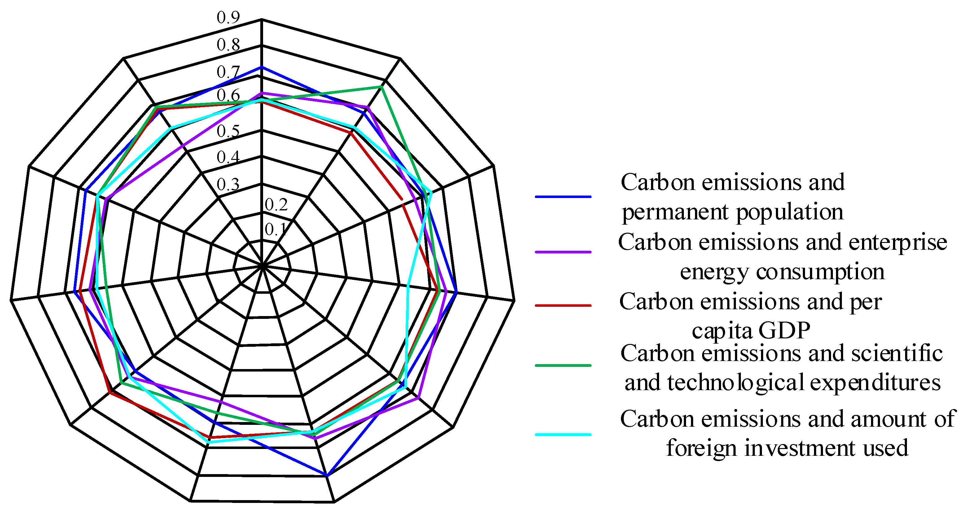
4.1. Analysis of Correlation Results of CE-Influencing Factors in Industrialized Rural Areas

Shandong Province is a region with a relatively fast development speed, a high degree of openness to the outside world, and a strong innovation driven effect in China. It plays an important role in the country’s four modernizations and the expansion of opening up to the outside world, plays an important role in national development, and has a significant influence nationwide. This article selects Luergang Village, Zhaowangzhuang Town, Laiyang City, Yantai City, Shandong Province; Hushan Village, Panshidian Town, Haiyang City, Yantai City, Shandong Province; Moujia Village, Fangyuan Street, Haiyang City, Yantai City, Shandong Province; Liugezhuang Village, Liugezhuang Town, Haiyang City, Yantai City, Shandong Province; Qiankuang Village, Guocheng Town, Haiyang City, Yantai City, Shandong Province; and Fangli Village, Liugezhuang Town, Haiyang City, Yantai City, Shandong Province, as the research objects, and the main energy consumption of each industrial sector category was selected from the 2005–2022 statistical yearbook. Meanwhile, the Moran’s I value calculation method was used for spatial correlation analysis.

From Figure 5, the cumulative contribution of CE brought about by the development effect of industrialized rural economy is the largest, which has played a promoting role in the increase of CE in the study area. Among them, the cumulative value between 2013 and 2022 reaches 5896 tons, and the contribution of the remaining three major factors to CO₂ emissions is negative, indicating that they have a significant inhibitory effect on CO₂ emissions. Among these influencing factors, the cumulative CE corresponding to the energy structure intensity effect, EC intensity effect, and population size effect are −6530 tons, −4558 tons, and −2780 tons, respectively.

Table 4. Spatial correlation analysis.

Industrial Functions	Year	Moran’s I	p-Value	Z-Score	Industrial Functions	Year	Moran’s I	p-Value	Z-Score
Industrial CE	2014	0.114	<0.05	6.3122	Living CE	2014	0.385	<0.05	21.9918
	2016	0.3	<0.05	8.3658		2016	0.31	<0.05	8.7669
	2018	0.263	<0.05	7.5172		2018	0.436	<0.05	11.834
	2020	0.048	<0.05	1.7253		2020	0.354	<0.05	13.7516
	2022	0.045	>0.05	1.4006		2022	0.202	<0.05	7.5203
Building CE	2014	0.19	<0.05	11.1912	Public CE	2014	−0.152	<0.05	−10.7103
	2016	0.331	<0.05	9.802		2016	−0.429	<0.05	−12.0519
	2018	0.134	<0.05	3.7417		2018	−0.401	<0.05	−11.5734
	2020	−0.065	<0.05	−3.0851		2020	−0.33	<0.05	−13.3907
	2022	0.03	>0.05	0.8669		2022	−0.43	<0.05	−14.2779
Commercial CE	2014	0.011	>0.05	−0.0584	CE from the transportation industry	2014	0.171	<0.05	10.1696
	2016	0.08	<0.05	2.252		2016	0.205	<0.05	6.1525
	2018	0.166	<0.05	4.7099		2018	0.273	<0.05	8.0469
	2020	0.353	<0.05	14.4168		2020	0.325	<0.05	13.795
	2022	0.356	<0.05	11.6346		2022	0.285	<0.05	9.9201

shows the spatial correlation analysis.

From Table 4, it can be seen that before dropping to 0.045 in 2020, the overall Moran index of industrial and CO₂ emissions increased from 0.114 in 2014 to 0.3. The p-values in 2014, 2016, and 2020 all reached a significance level of 5%, indicating a positive spatial correlation. But in 2022, its significance could not reach 5%, and Z was only 1.4006. This indicates that there is a trend of first increasing and then decreasing in the spatial aggregation of industrial functions and CE. And the overall Moran index between commercial and CO₂ emissions is also constantly increasing. Among them, the p-values between commercial functions and CE quantity in 2014 and 2016 are both below the 5% significant level, and show a trend from randomness to clustering spatially.

In Figure 6, from 2007 to 2022, overall, the correlation between CE quantity in the study area and the three influencing factors of science and technology expenditure, external funds, and corporate energy EC gradually increased. Overall, there was a decreasing trend in the correlation between the permanent population and per capita GDP in various regions and CO₂ emissions. From a local perspective, the relationship between enterprise energy EC and per capita GDP and rural industrial CE had a high volatility correlation. In 2012, 2016, and 2021, there was a significant reversal between per capita GDP and CO₂ emissions in the region. From 2008 to 2010 and 2014, the correlation between corporate EC and CO₂ emissions underwent significant changes. In 2020, in addition to the per capita GDP indicator, the correlation between various influencing factors and CE volume showed a decreasing trend, indicating that low-carbon development had achieved certain results in recent years.

From Figure 7, it can be seen that in terms of the correlation between carbon emissions and permanent population, the highest value is 0.72; the highest value in the correlation between carbon emissions and enterprise energy consumption is 0.73. The correlation between rural areas and per capita GDP in most cities is above 0.6.

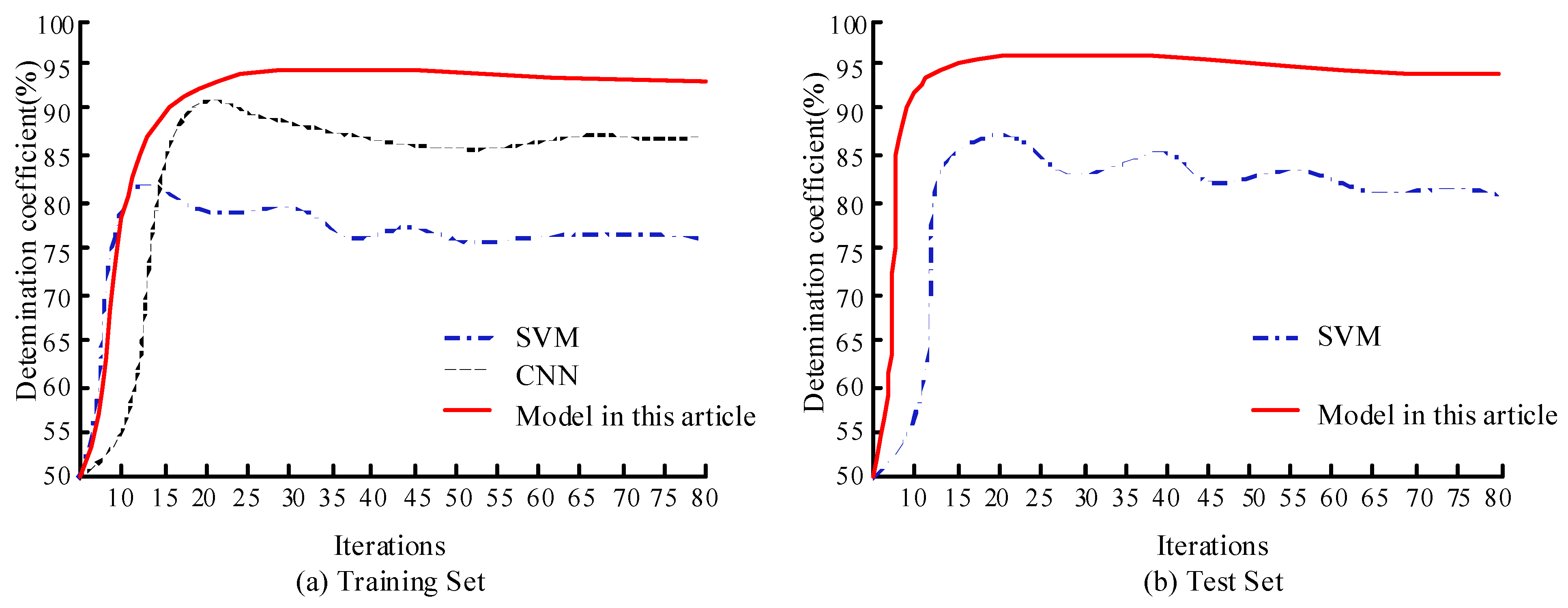
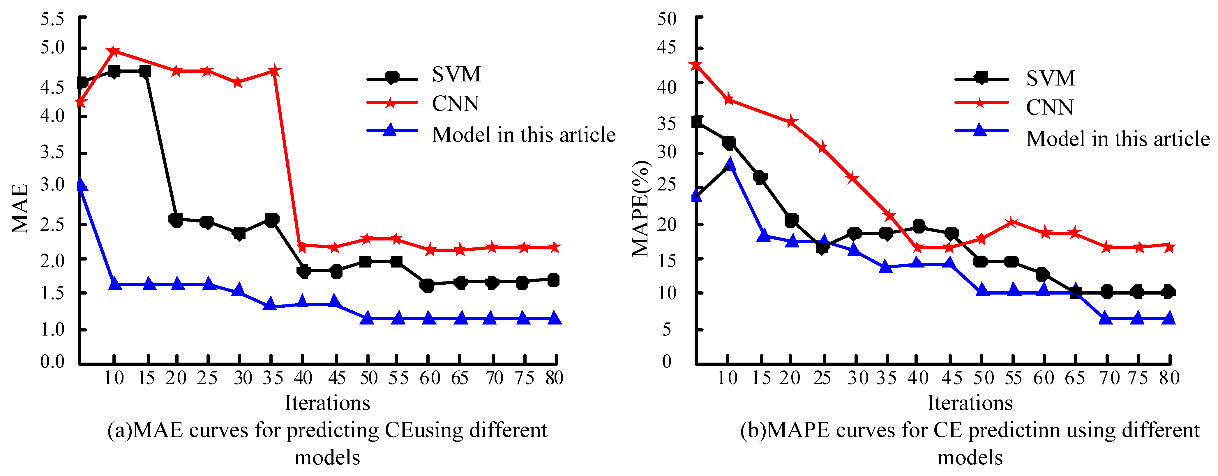
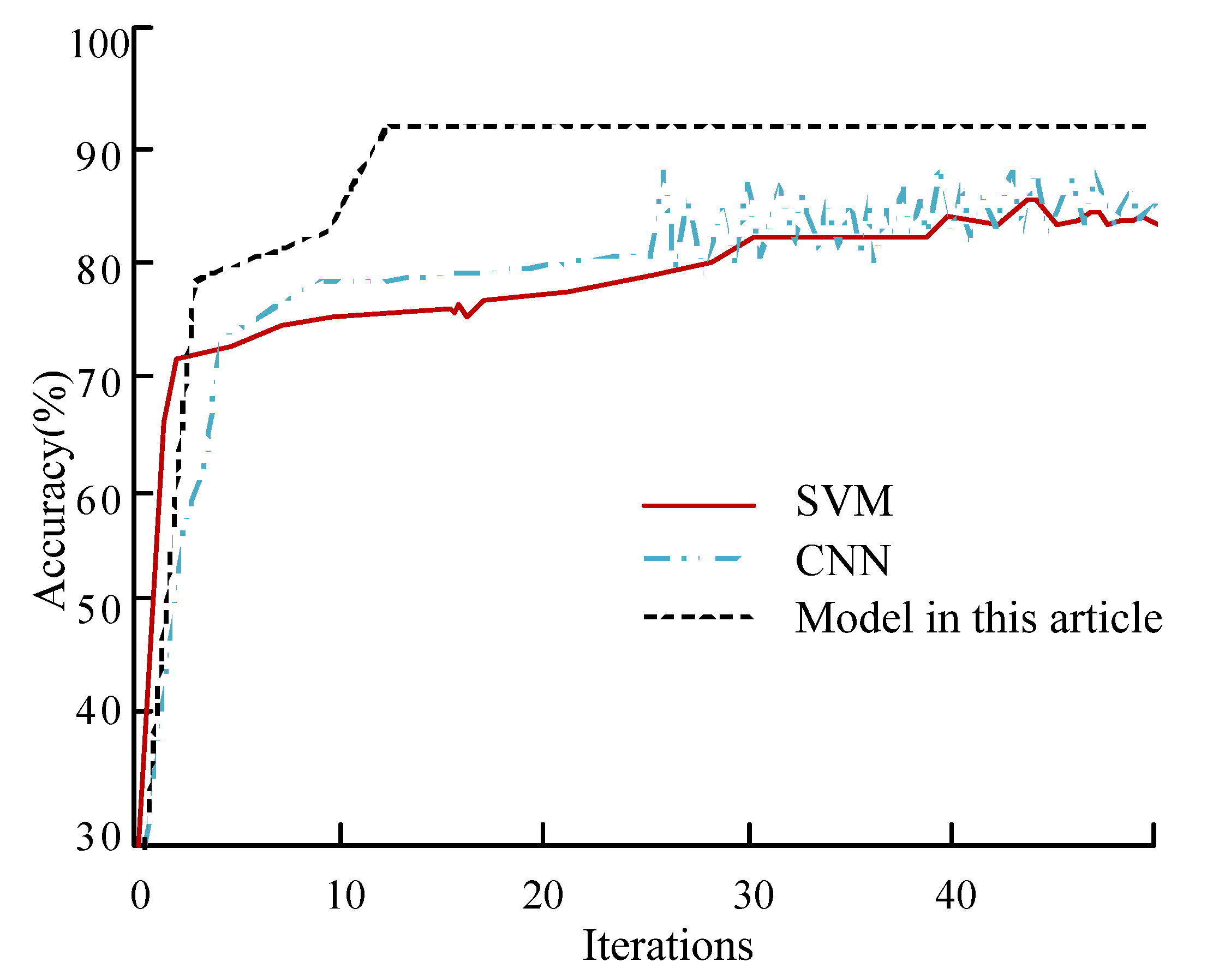
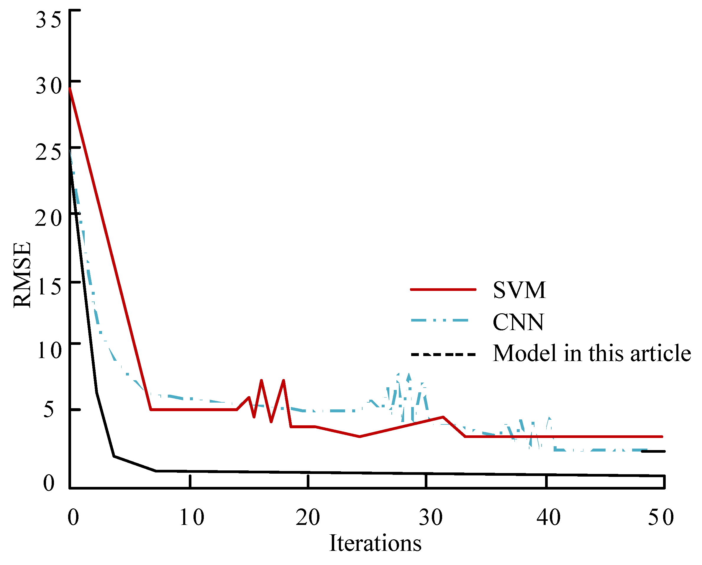
4.2. Effectiveness Analysis of CE Prediction Model

After converting and normalizing the data, the dataset was divided into training and testing sets in a 7:3 ratio. The evaluation indicators of the model include coefficient of determination, root mean square error (RMSE), mean absolute error (MAE), and mean absolute percentage error (MAPE). If MAPE is 0, it indicates that the model has the best performance. If MAPE is greater than 100%, it indicates that the model has poor performance. In contrast, MAE and MAPE are less susceptible to extreme values. And RMSE makes it more sensitive to abnormal data by multiplying the error by the square of the error. Compared to other indicators, MAPE uses percentages to measure the degree of error.

In Figure 8a, as the iteration increases, the decision coefficient curve of the proposed CE prediction model on the training set becomes smoother, with smaller fluctuations, and the final convergence value obtained was the highest, with a size of 92.6%. SVM and CNN prediction models have higher fluctuation frequency and amplitude, and their convergence speed and value are lower than those of this model. The convergence values of the determination coefficients for the latter two models were 75.2% and 87.3%, respectively. After comparison, the proposed algorithm improved the convergence value of the coefficient by 17.4% and 5.3% compared to them. From Figure 8b, on the test set, this proposed model begins to converge at iteration 15. Although there is a slight decrease during the iteration, the overall curve does not fluctuate, resulting in a convergence value of 94.8%. The CNN prediction model, on the other hand, has a higher initial convergence time and significant fluctuations, resulting in a convergence value of 88.6%. These all indicate that the proposed algorithm has higher accuracy in CE prediction.

In Figure 9a, the MAE of the proposed prediction model shows a rapid decline and tends to converge steadily. When the iteration is 10, the model begins to enter the convergence stage. When the iteration is 80, the model obtains a final convergence value of 1.18. The SVM and CNN used for comparison have a certain upward trend in the early stages of iteration, and there are significant fluctuations in the middle stage. The latter two models both tend to converge at around 40 iterations, with final convergence values of 1.68 and 2.24, both lower than the proposed model. In Figure 9b, the MAPE of the proposed model shows a stepwise downward trend, first decreasing at iteration 10 and achieving a convergence value of 6.8 at iteration 70. However, SVM and CNN have a certain upward range in the middle of the iteration, and their final convergence values are also higher than the proposed model, with values of 16.9 and 10.1, respectively. Therefore, these indicate that the proposed model has smaller prediction errors.

From Figure 10, the accuracy of the three prediction models shows an increasing trend. However, the proposed model begins to converge at iteration 12, and the final convergence value obtained at the completion of the iteration is 91.6%. Although SVM and CNN are in a relatively stable climbing stage in the early stages of iteration, their accuracies begin to fluctuate significantly with the increase of iteration, and they ultimately fail to obtain convergence values.

From Figure 11, the RMSE of the proposed model decreases the fastest and the convergence stage is the most stable. When the iteration is 50, it obtains a final RMSE of 0.89. However, SVM and CNN prediction models have a larger slope in the descent stage, more fluctuations in the iteration stage, and ultimately obtain a larger RMSE.

5. Conclusions

As urbanization continues to advance, economic development also brings huge environmental problems, and the surge in CE quantity has made the greenhouse gas effect more significant. To reduce industrial pollution in cities, many industries choose to relocate factories to rural areas. This study constructed a GRA-based CE influencing factor analysis method and an ST-GCN-based CE prediction model to analyze the correlation degree and prediction effect of carbon-driving factors in industrialized rural areas. These results confirmed that in the test set, the proposed model began to converge at iteration 15. Despite some slight attenuation during the iteration, the overall curve remained stable, and the final convergence value reached 94.8%. However, CNN had a longer initial convergence period and significant volatility, ultimately reaching only 88.6% of the convergence value. In addition, the MAPE of the proposed model exhibited significant attenuation at iteration 10, and its convergence reached 6.8 at iteration 70. The MAPE values of the control group were all above 10. These results confirmed that this model had high prediction accuracy and could better reflect the actual situation. Li R et al. studied the impact on carbon emissions from four aspects: energy, trade, society, and economy, taking into account economic growth and energy intensity. Their results show that economic growth and increased energy intensity promote an increase in carbon emissions, while increasing renewable energy consumption helps to reduce carbon emissions. They also proposed policy recommendations to reduce per capita carbon emissions by adjusting the economic, energy, social, and trade structures [41]. Li Y et al. used panel data from 30 provinces in China from 2011 to 2017 to empirically test the impact of energy structure and digital economy on carbon emissions. The results indicate that the energy structure dominated by coal has a significant driving effect on carbon emissions. Compared with non-resource-based provinces, the increase in energy structures dominated by coal has a greater impact on carbon emissions in resource-based provinces [42]. Carbon emissions are greatly affected by GDP. At the level of economic development, increasing economic cooperation between provinces and cities is necessary to change the economic development model, increase efforts to develop a low-carbon economy, establish economic development goals of low energy consumption and low pollution, and improve energy utilization efficiency and implement technological innovation through the achievement of these goals. The transformation process of high-energy-consuming industries is vital. Only by developing clean energy technologies and using renewable energy, and changing and developing energy from multiple aspects, can we promote the transformation of energy consumption structures. This can be achieved by actively promoting research on carbon reduction-related technologies, researching and developing low-carbon clean energy technologies, and jointly seeking a green development path. Research also requires funding, and the government needs to focus on researchers, increase investment in carbon reduction-related technology research, and actively innovate related technologies such as energy conversion and improving utilization efficiency. By expanding the research scope of this article, from Shandong Province to surrounding provinces and cities, and finally to the entire country, to conduct in-depth research on the economic development, energy consumption, and carbon emissions of various provinces and cities across the country, only in this way can we more accurately predict the peak time of China’s carbon emissions and grasp the achievement of China’s “dual carbon” goals, providing policy recommendations and theoretical basis for China’s carbon reduction work.

References

1. Duarte, A.J.; Malheiro, B.; Arnó, E.; Perat, I.; Silva, M.F.; Fuentes-Durá, P.; Guedes, P.; Ferreira, P. Engineering education for sustainable development: The European project semester approach. IEEE Trans. Educ. 2020, 63, 108–117. [Google Scholar] [CrossRef]
2. Mai, V.; Vanderborght, B.; Haidegger, T.; Khamis, A.; Bhargava, N.; Boesl, D.B.O.; Gabriels, K.; Jacobs, A.; Moon, A.; Murphy, R.; et al. The role of robotics in achieving the united nations sustainable development goals—The experts’ meeting at the 2021 IEEE/RSJ IROS workshop. IEEE Robot. Autom. Mag. 2022, 29, 92–107. [Google Scholar] [CrossRef]
3. Liu, Q.; Sun, S.L.; Rong, B.; Kadoch, M. Intelligent reflective surface based 6g communications for sustainable energy infrastructure. IEEE Wirel. Commun. 2021, 28, 49–55. [Google Scholar] [CrossRef]
4. Pao, H.T.; Fu, H.C.; Tseng, C.L. Forecasting of CO2 emissions, energy consumption and economic growth in China using an improved grey model. Energy 2012, 41, 400–409. [Google Scholar] [CrossRef]
5. Ding, T.; Jia, W.H.; Shahidehpour, M.; Han, O.Z.; Sun, Y.G.; Zhang, Z.Y. Review of optimization methods for energy hub planning, operation, trading, and control. IEEE Trans. Sustain. Energy 2022, 13, 1802–1818. [Google Scholar] [CrossRef]
6. Li, Y.; Han, M.; Yang, Z.; Li, G.Q. Coordinating flexible demand response and renewable uncertainties for scheduling of community integrated energy systems with an electric vehicle charging station: A bi-level approach. IEEE Trans. Sustain. Energy 2021, 12, 2321–2331. [Google Scholar] [CrossRef]
7. Zhang, Y.X.; Xu, Y.; Yang, H.M.; Dong, Z.Y.; Zhang, R. Optimal whole-life-cycle planning of battery energy storage for multi-functional services in power system. IEEE Trans. Sustain. Energy 2020, 11, 2077–2086. [Google Scholar] [CrossRef]
8. Xu, D.; Wu, Q.W.; Zhou, B.; Li, C.B.; Bai, L.; Huang, S. Distributed multi-energy operation of coupled electricity, heating, and natural gas networks. IEEE Trans. Sustain. Energy 2020, 11, 2457–2469. [Google Scholar] [CrossRef]
9. Li, Y.; Wang, R.N.; Yang, Z. Optimal scheduling of isolated microgrids using automated reinforcement learning-based multi-period forecasting. IEEE Trans. Sustain. Energy 2022, 13, 159–169. [Google Scholar] [CrossRef]
10. Brown, D. Towards a comparative research agenda on in situ urbanisation and rural governance transformation. Int. Dev. Plan. Rev. 2021, 43, 289–320. [Google Scholar] [CrossRef]
11. Bhuvana, M.; Vasantha, S. Assessment of rural citizens satisfaction on the service quality of common service centers (CSCs) of e-governance. J. Crit. Rev. 2020, 7, 302–305. [Google Scholar] [CrossRef]
12. Yaacoub, E.; Alouini, M.S. A key 6g challenge and opportunity—Connecting the base of the pyramid: A survey on rural connectivity. Proc. IEEE 2020, 108, 533–582. [Google Scholar] [CrossRef]
13. Yaacoub, E.; Alouini, M.S. Efficient Fronthaul and Backhaul Connectivity for IoT Traffic in Rural Areas. IEEE Internet Things Mag. 2021, 4, 60–66. [Google Scholar] [CrossRef]
14. Kirikkaleli, D.; Adebayo, T.S. Do public-private partnerships in energy and renewable energy consumption matter for consumption-based carbon dioxide emissions in India? Environ. Sci. Pollut. Res. 2021, 28, 30139–30152. [Google Scholar] [CrossRef] [PubMed]
15. Dong, K.Y.; Dong, X.C.; Jiang, Q.Z. How renewable energy consumption lower global CO2 emissions? Evidence from countries with different income levels. World Econ. 2020, 43, 1665–1698. [Google Scholar] [CrossRef]
16. Murad, M.W.; Alam, M.M.; Noman, A.H.M.; Ozturk, I. Dynamics of technological innovation, energy consumption, energy price and economic growth in Denmark. Environ. Prog. Sustain. Energy 2019, 38, 22–29. [Google Scholar] [CrossRef]
17. Wei, Z.Q.; Wei, K.K.; Liu, J.C. Decoupling relationship between carbon emissions and economic development and prediction of carbon emissions in Henan Province: Based on Tapio method and STIRPAT model. Environ. Sci. Pollut. Res. 2023, 30, 52679–52691. [Google Scholar] [CrossRef] [PubMed]
18. Liu, Y.N.; Wei, X.X.; Xiao, J.Y.; Liu, Z.H.J.; Xu, Y.; Tian, Y. Energy consumption and emission mitigation prediction based on data center traffic and PUE for global data centers. Glob. Energy Int. 2020, 3, 272–282. [Google Scholar] [CrossRef]
19. Adame, M.F.; Connolly, R.M.; Turschwell, M.P.; Lovelock, C.E.; Fatoyinbo, T.; Lagomasino, D.; Goldberg, L.A.; Holdorf, J.; Friess, D.A.; Sasmito, S.D.; et al. Future carbon emissions from global mangrove forest loss. Glob. Chang. Biol. 2021, 27, 2856–2866. [Google Scholar] [CrossRef] [PubMed]
20. Yu, Y.; Du, Y. Impact of technological innovation on CO2 emissions and emissions trend prediction on ‘New Normal’ economy in China. Atmos. Pollut. Res. 2019, 10, 152–161. [Google Scholar] [CrossRef]
21. Ran, Q.Y.; Bu, F.B.; Razzaq, A.; Ge, W.F.; Peng, J.; Yang, X.D.; Xu, Y. When will China’s industrial carbon emissions peak? Evidence from machine learning. Environ. Sci. Pollut. Res. 2023, 30, 57960–57974. [Google Scholar] [CrossRef] [PubMed]
22. Lv, T.G.; Hu, H.; Xie, H.L.; Zhang, X.M.; Wang, L.; Shen, X.Q. An empirical relationship between urbanization and carbon emissions in an ecological civilization demonstration area of China based on the STIRPAT model. Environ. Dev. Sustain. 2023, 25, 2465–2486. [Google Scholar] [CrossRef]
23. Jin, I. Probability of achieving NDC and implications for climate policy: CO-STIRPAT approach. J. Econ. Anal. 2023, 2, 82–97. [Google Scholar] [CrossRef]
24. Pan, G.S.; Gu, W.; Lu, Y.P.; Qiu, H.F.; Lu, S.; Yao, S. Optimal planning for electricity-hydrogen integrated energy system considering power to hydrogen and heat and seasonal storage. IEEE Trans. Sustain. Energy 2020, 11, 2662–2676. [Google Scholar] [CrossRef]
25. Hu, J.J.; Liu, X.T.; Shahidehpour, M.; Xia, S.W. Optimal operation of energy hubs with large-scale distributed energy resources for distribution network congestion management. IEEE Trans. Sustain. Energy 2021, 12, 1755–1765. [Google Scholar] [CrossRef]
26. Li, Z.W.; Cheng, Z.P.; Liang, J.; Si, J.K.; Dong, L.H.; Li, S.H. Distributed event-triggered secondary control for economic dispatch and frequency restoration control of droop-controlled ac microgrids. IEEE Trans. Sustain. Energy 2020, 11, 1938–1950. [Google Scholar] [CrossRef]
27. Lu, R.Z.; Ding, T.; Qin, B.Y.; Ma, J.; Fang, X.; Dong, Z.Y. Multi-stage stochastic programming to joint economic dispatch for energy and reserve with uncertain renewable energy. IEEE Trans. Sustain. Energy 2020, 11, 1140–1151. [Google Scholar] [CrossRef]
28. Yu, D.M.; Ebadi, A.G.; Jermsittiparsert, K.; Jabarullah, N.H.; Vasiljeva, M.V.; Nojavan, S. Risk-constrained stochastic optimization of a concentrating solar power plan. IEEE Trans. Sustain. Energy 2020, 11, 1464–1472. [Google Scholar] [CrossRef]
29. Guo, Z.J.; Wei, W.; Chen, L.J.; Dong, Z.Y.; Mei, S.W. Impact of energy storage on renewable energy utilization: A geometric description. IEEE Trans. Sustain. Energy 2021, 12, 874–885. [Google Scholar] [CrossRef]
30. Hua, H.C.; Qin, Z.M.; Dong, N.Q.; Qin, Y.C.; Ye, M.J.; Wang, Z.D.; Chen, X.Y.; Cao, J.W. Data-driven dynamical control for bottom-up energy internet system. IEEE Trans. Sustain. Energy 2022, 13, 315–327. [Google Scholar] [CrossRef]
31. Zheng, Y.; Song, Y.; Huang, A.D.; Hill, D.J. Hierarchical optimal allocation of battery energy storage systems for multiple services in distribution systems. IEEE Trans. Sustain. Energy 2020, 11, 1911–1921. [Google Scholar] [CrossRef]
32. Ge, L.J.; Liu, H.X.; Yan, J.; Zhu, X.S.; Zhang, S.; Li, Y.Z. Optimal integrated energy system planning with dg uncertainty affine model and carbon emissions charges. IEEE Trans. Sustain. Energy 2022, 13, 905–918. [Google Scholar] [CrossRef]
33. Wang, Y.Q.; Qiu, J.; Tao, Y.C.; Zhao, J.H. Carbon-oriented operational planning in coupled electricity and emission trading markets. IEEE Trans. Power Syst. 2020, 35, 3145–3157. [Google Scholar] [CrossRef]
34. Wei, X.; Zhang, X.; Sun, Y.X.; Qiu, J. Carbon emission flow oriented tri-level planning of integrated electricity–hydrogen–gas system with hydrogen vehicles. IEEE Trans. Ind. Appl. 2021, 58, 2607–2618. [Google Scholar] [CrossRef]
35. Bao, J.B.; He, D.B.; Luo, M.; Choo, K.K.R. A survey of blockchain applications in the energy sector. IEEE Syst. J. 2021, 15, 3370–3381. [Google Scholar] [CrossRef]
36. Yang, L.F.; Luo, J.Y.; Xu, Y.; Zhang, Z.R.; Dong, Z.Y. A distributed dual consensus admm based on partition for dc-dopf with carbon emission trading. IEEE Trans. Ind. Inform. 2020, 16, 1858–1872. [Google Scholar] [CrossRef]
37. Cheng, Y.H.; Zhang, N.; Zhang, B.S.; Kang, C.Q.; Xi, W.M.; Feng, M.S. Low-Carbon operation of multiple energy systems based on energy-carbon integrated prices. IEEE Trans. Smart Grid 2020, 11, 1307–1318. [Google Scholar] [CrossRef]
38. Patterson, D.; Gonzalez, J.; Hölzle, U.; Le, Q.; Liang, C.; Munguia, L.M.; Rothchild, D.; So, D.R.; Texier, M.; Dean, J. The carbon footprint of machine learning training will plateau, then shrink. Computer 2022, 55, 18–28. [Google Scholar] [CrossRef]
39. Yan, M.Y.; Shahidehpour, M.; Alabdulwahab, A.; Abusorrah, A.; Gurung, N.; Zheng, H.H.; Ogunnubi, O.; Vukojevic, A.; Paaso, E.A. Blockchain for transacting energy and carbon allowance in networked microgrids. IEEE Trans. Smart Grid 2021, 12, 4702–4714. [Google Scholar] [CrossRef]
40. Huang, W.J.; Zhang, N.; Cheng, Y.H.; Yang, J.W.; Wang, Y.; Kang, C.Q. Multienergy networks analytics: Standardized modeling, optimization, and low carbon analysis. Proc. IEEE 2020, 108, 1411–1436. [Google Scholar] [CrossRef]
41. Li, R.; Wang, Q.; Liu, Y.; Jiang, R. Per-capita carbon emissions in 147 countries: The effect of economic, energy, social, and trade structural changes. Sustain. Prod. Consum. 2021, 27, 1149–1164. [Google Scholar] [CrossRef]
42. Li, Y.; Yang, X.; Ran, Q.; Wu, H.T.; Irfan, M.; Ahmad, M. Energy structure, digital economy, and carbon emissions: Evidence from China. Environ. Sci. Pollut. Res. 2021, 28, 64606–64629. [Google Scholar] [CrossRef] [PubMed]
Figure 1. Schematic diagram of grey correlation analysis.
Sustainability 15 16750 g001
Figure 2. Schematic diagram of graph theory.
Sustainability 15 16750 g002
Figure 3. Topological relationships of unauthorized networks.
Sustainability 15 16750 g003
Figure 4. Schematic diagram of spatiotemporal graph convolution model.
Sustainability 15 16750 g004
Figure 5. Accumulated variation value of CE-influencing factors.
Sustainability 15 16750 g005
Figure 6. Time series grey correlation degree.
Sustainability 15 16750 g006
Figure 7. Cross-section grey correlation degree.
Sustainability 15 16750 g007
Figure 8. Coefficient curves determined by different models.
Sustainability 15 16750 g008
Figure 9. MAE and MAPE curves for CE prediction using different models.
Sustainability 15 16750 g009
Figure 10. Accuracy curves of CE prediction for different models.
Sustainability 15 16750 g010
Figure 11. RMSE curves for carbon emission prediction using different models.
Sustainability 15 16750 g011