Article

Optimal Operation of Distribution Networks Considering Renewable Energy Sources Integration and Demand Side Response

1
Electrical Engineering Laboratory, University of Kasdi Merbah, Ouargla 30000, Algeria
2
IREENA Laboratory, Nantes University, 44035 Nantes, France
3
Department of Electrical Engineering, Faculty of Engineering, Sohag University, Sohag 82524, Egypt
4
LACoSERE Laboratory, University of Amar Telidji, Laghouat 03000, Algeria
*
Author to whom correspondence should be addressed.
Sustainability 2023, 15(24), 16707; https://doi.org/10.3390/su152416707
Submission received: 16 October 2023 / Revised: 19 November 2023 / Accepted: 7 December 2023 / Published: 10 December 2023

Abstract

:
This paper demonstrates the effectiveness of Demand Side Response (DSR) with renewable integration by solving the stochastic optimal operation problem (OOP) in the IEEE 118-bus distribution system over 24 h. An Improved Walrus Optimization Algorithm (I-WaOA) is proposed to minimize costs, reduce voltage deviations, and enhance stability under uncertain loads, generation, and pricing. The proposed I-WaOA utilizes three strategies: the fitness-distance balance method, quasi-opposite-based learning, and Cauchy mutation. The I-WaOA optimally locates and sizes photovoltaic (PV) ratings and wind turbine (WT) capacities and determines the optimal power factor of WT with DSR. Using Monte Carlo simulations (MCS) and probability density functions (PDF), the uncertainties in renewable energy generation, load demand, and energy costs are represented. The results show that the proposed I-WaOA approach can significantly reduce costs, improve voltage stability, and mitigate voltage deviations. The total annual costs are reduced by 91%, from 3.8377 × 10⁷ USD to 3.4737 × 10⁶ USD. Voltage deviations are decreased by 63%, from 98.6633 per unit (p.u.) to 36.0990 p.u., and the system stability index is increased by 11%, from 2.444 × 10³ p.u. to 2.7245 × 10³ p.u., when contrasted with traditional methods.

1. Introduction

1.1. Motivation

In recent years, the reliability of energy supplies to consumers has gained paramount significance. This is owing to its role as a pivotal determinant of both capacity quality and customer satisfaction within distribution networks. Enterprises wield a plethora of options to enhance distribution network reliability, including the utilization of Renewable Energy Sources (RESs). RESs, like wind and solar power, present promising low-carbon substitutes for conventional fossil fuels [1,2]. Nevertheless, the intermittent and uncertain characteristics of RESs present complex hurdles to grid design. To tackle these challenges, the integration of RESs and the implementation of Demand Side Management strategies come to the forefront. DSR, comprising compact power facilities located proximately to the point of consumption, holds the capacity to alleviate strain on centralized networks and bolster resilience through fault isolation for swift recovery from downtimes. Complementary to this, DSR techniques like real-time pricing (RTP) exhibit the potential to reduce energy consumption during peak demand intervals. Collaboratively, the synergy of RESs and DSR stands poised to revamp the distribution system, allowing for a substantial integration of renewable energy. This transformation is indispensable for steering toward a sustainable energy future [3,4].

1.2. Related Work

Several studies have been carried out on the integration of renewable energies into electrical networks. For example, the authors in [5] present a novel and effective approach to the ideal siting and dimensioning of PV resources in distribution networks. In [6], a hybrid Harmony Search Algorithm approach is proposed to enhance bus voltage profiles and minimize power losses in the distribution network (DN). Integrating the Particle Artificial Bee Colony algorithm with Harmony Search addresses convergence issues. The hybrid algorithm determines optimal locations and sizes for distributed generators and capacitor banks (CB), proving superior loss reduction compared to current methods in the literature on test systems with 33 and 119 nodes. The authors in [7] present a method for optimal placement and sizing of PV and WT in distribution networks. Their approach, using a weighted aggregation Particle Swarm Optimization technique, addresses power loss minimization, voltage stability, and network security while considering the stochastic nature of renewable resources. Applied to an Indian rural distribution network, the method showcases effective enhancement of network operational benefits. In [8], a reinforcement learning-based method is proposed for optimal sizing of PV sources in unbalanced distribution networks, considering uncertainty and seasonal variations. The technique is validated on IEEE 13- and 37-bus feeders and is shown to be suitable for real-system implementation. The paper [9] addresses various technological challenges related to stability issues associated with high PV penetration into the power grid. These challenges include frequency regulation, active power reduction, reactive power injection, and energy storage. In [10], ramp-rate control algorithms have been proposed to minimize grid power fluctuations by using energy storage systems. The technical challenges arising from the extensive integration of PV systems into the electrical grid, like voltage limit violations and frequency disturbances, are explored in [11]. The optimal network reconfiguration is obtained using an enhanced whale optimization approach [12]. The mine blast method is used to find the best location and size of CB in DN [13] and the grey wolf optimization method [14]. The ant lion optimization algorithm in [15] is suggested for the best RES sizing and allocation in DN. The authors of the paper [16] have proposed a new method for optimal placement and sizing of RESs in DN, considering the uncertainties of RESs output powers and loading. In [17], the Salp Swarm Algorithm is applied to optimize the allocation of WT in DN to reduce overall energy and power loss. This approach supports the integration of commercially available renewable energy technologies, particularly wind turbines, and responds to global environmental concerns. In [18], the authors introduce a novel methodology, HHO-PSO, for optimizing the planning of RESs in active distribution systems. The results demonstrated that HHO-PSO provides superior solutions, maximizing techno-economic benefits. In [19], the authors propose a new algorithm for optimal allocation of distributed generation units in radial distribution networks. The proposed algorithm, called AEO-OBL, is a modified form of the optimization method modeled on artificial ecosystems. The authors in [20] propose an effective RESs allocation strategy for energy loss minimization in the presence of variable power demand. In [21], the study introduces a hybrid stochastic-IGDT strategy to improve the resilient functioning of intelligent DN with the incorporation of RESs and intelligent parking facilities. A comprehensive integration of storage approaches for the OOP of energy storage systems is proposed in DN [22]. In [23], a method is presented for concurrent positioning of distribution static compensators, RESs, and DN reconfiguration using stochastic multi-objective optimization. The problem is formulated as a mixed-integer, nonlinear programming problem. The authors in [24] propose a new approach for the optimal siting and sizing of wind turbines and devices for storing energy in distribution networks. The suggested methodology takes into account the impact of WTs on power quality, specifically flicker emission. In [4], the authors propose a technique for improving the reliability of DN using DSR programs and smart charging/discharging of plug-in electric vehicles (PEV). In [25], a DSR mechanism is introduced to enable energy consumers to adjust their energy consumption patterns as proposed. The authors in [26] study the potential benefits of DSR resources for distribution networks. They consider two different types of customers: residential and commercial. They install data loggers on two real distribution feeders in Golpayegan city and collect load profiles. They then use these load profiles to develop two DSR programs: time-of-use and emergency DSR. They apply the DSR programs to the real network and simulate the system using the CYME software. In [27], the authors address the uncertainties introduced by the stochastic nature of RESs and DSR in distribution grids. The authors in [28] present a novel darts game theory-based optimization algorithm for microgrid formation, considering multiple objectives, topological and electrical constraints, and demand response. The modified IEEE 33-bus test system is used to validate the suggested methodology, demonstrating its superiority over existing methods and its potential to improve system resiliency under extreme events.
The addition of Cauchy mutations to optimization algorithms has been shown to improve their capability to address intricate global engineering optimization challenges. This enhancement leads to the discovery of better optimal solutions, as has been demonstrated by many research studies [29]. Furthermore, the refinement of optimization performance is achievable through the harmonization of fitness and distance considerations within the search process. This improvement has been substantiated through a diverse array of research inquiries [30].
In this context, quasi-opposite-based learning (QOBL) emerges as a widely adopted strategy to amplify population diversity within optimization algorithms. Proposed as an extension of the opposition-based learning approach, QOBL operates on a similar premise, involving the evaluation of agents at their opposite points within the parameter space. QOBL extends this principle by uniformly assessing points selected along a straight line connecting the search space’s center with the opposing point of the agent’s current location. The viability of QOBL holds promise for further enriching optimization algorithms’ performance and diversification strategies, contributing to a holistic advancement in engineering optimization techniques [31]. Table 1 summarizes the work given and compares it to other relevant research on the optimal operation of DN with RESs.

1.3. Contribution

As evident, the literature on addressing the OOP is extensive. However, to our knowledge, only a limited number of studies have tackled the stochastic OOP with optimal WT and solar PV system integration along with DSR while accounting for uncertainties in wind speed fluctuations, load, temperature shifts, variations in solar irradiation, and the volatility of energy purchasing prices. In summary, the research gaps identified in these studies are outlined below:
  • References [5,6,7] identified the optimal locations for PV and WT, but the shortcoming in these studies is the lack of consideration for uncertainty and DSR.
  • References [8,17,18,32,33] explored the issue of OOP, taking into consideration uncertainties in load, radiation, and wind speed. However, these studies omitted uncertainties related to temperatures and prices. Additionally, the Demand Side Response was not considered in these studies.
  • References [4,27,28] investigated the optimal operation problem (OOP) while relying exclusively on Demand Side Response to enhance the performance of the electrical distribution network. However, a limitation of these studies is the lack of consideration for all uncertainties within the system.
In this study, we investigate the impact of integrating a system comprising photovoltaic generators and wind turbines in conjunction with Demand Side Response. We introduce a novel approach termed the Improved Walrus Optimization Algorithm, aiming to address the optimization challenge within the IEEE 118 Distribution Network. Our primary objective is twofold: to reduce costs and voltage deviations (VD) while enhancing the voltage stability index (VSI) for the duration of a day. The effectiveness of the model is carefully evaluated, taking uncertainties into account in wind speed fluctuations, load, temperature shifts, variations in solar irradiation, and the volatility of energy purchasing prices. We compare our proposed method (I-WaOA) against established optimization techniques, including Sand Cat swarm optimization (SCSO), Artificial Hummingbird Algorithm (AHA), Dandelion Optimizer (DO), Harmony Search (HS), Artificial Rabbits Optimization (ARO), Chernobyl Disaster Optimizer (CDO), Zebra Optimization Algorithm (ZOA), and standard Walruses behavior (WaOA).
Figure 1 represents the graphical summary of this paper, incorporating the integration of RESs with DSR in line with the DN of impedance R i , j + j X i , j connected between buses i and j.
The key accomplishments of this research can be summarized as follows:
  • A novel Improved Walrus Optimization Algorithm (I-WaOA) is proposed to solve the optimal operation problem (OOP) of renewable energy resources (RESs) with Demand Side Response (DSR) in distribution networks (DN).
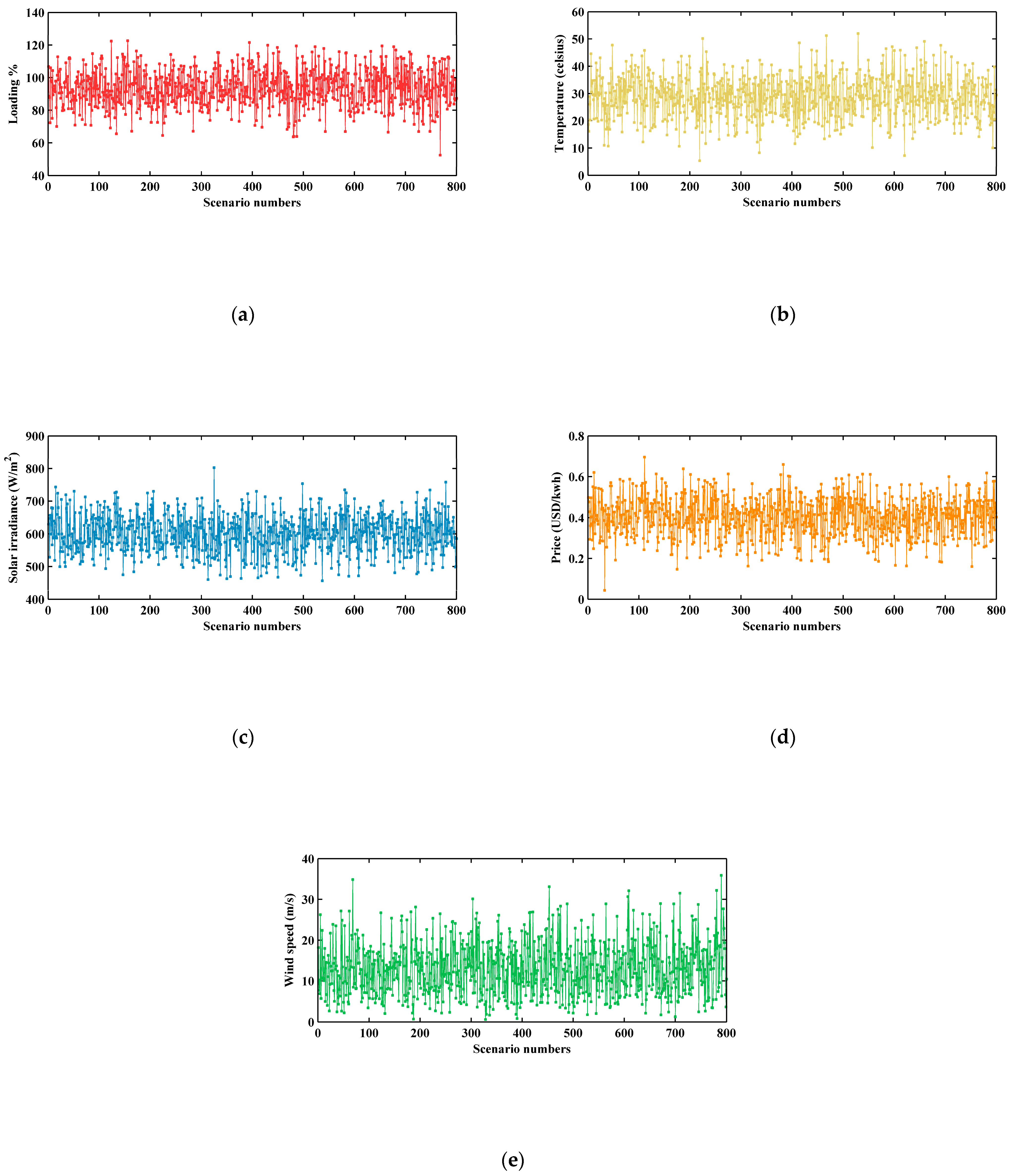
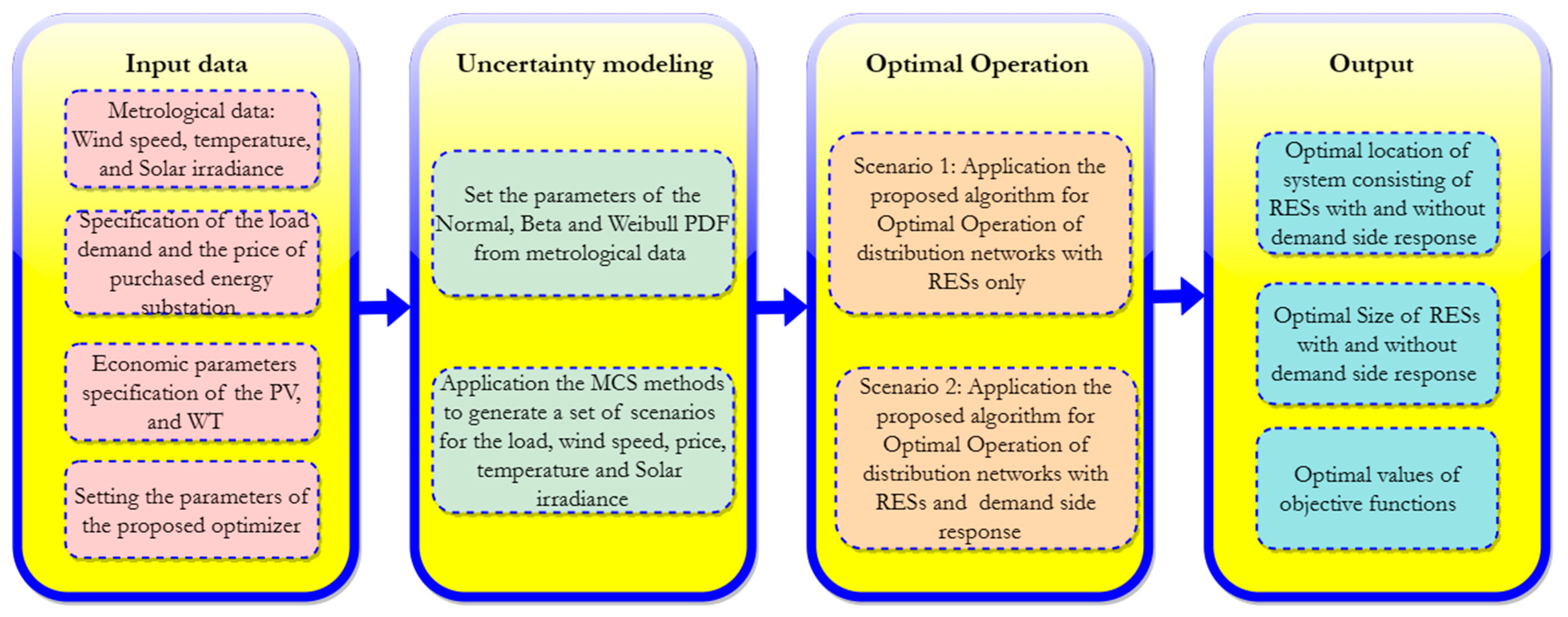
  • The uncertainties related to load demand, RESs generation, temperature, and energy pricing are represented through PDF and simulated using MCS.
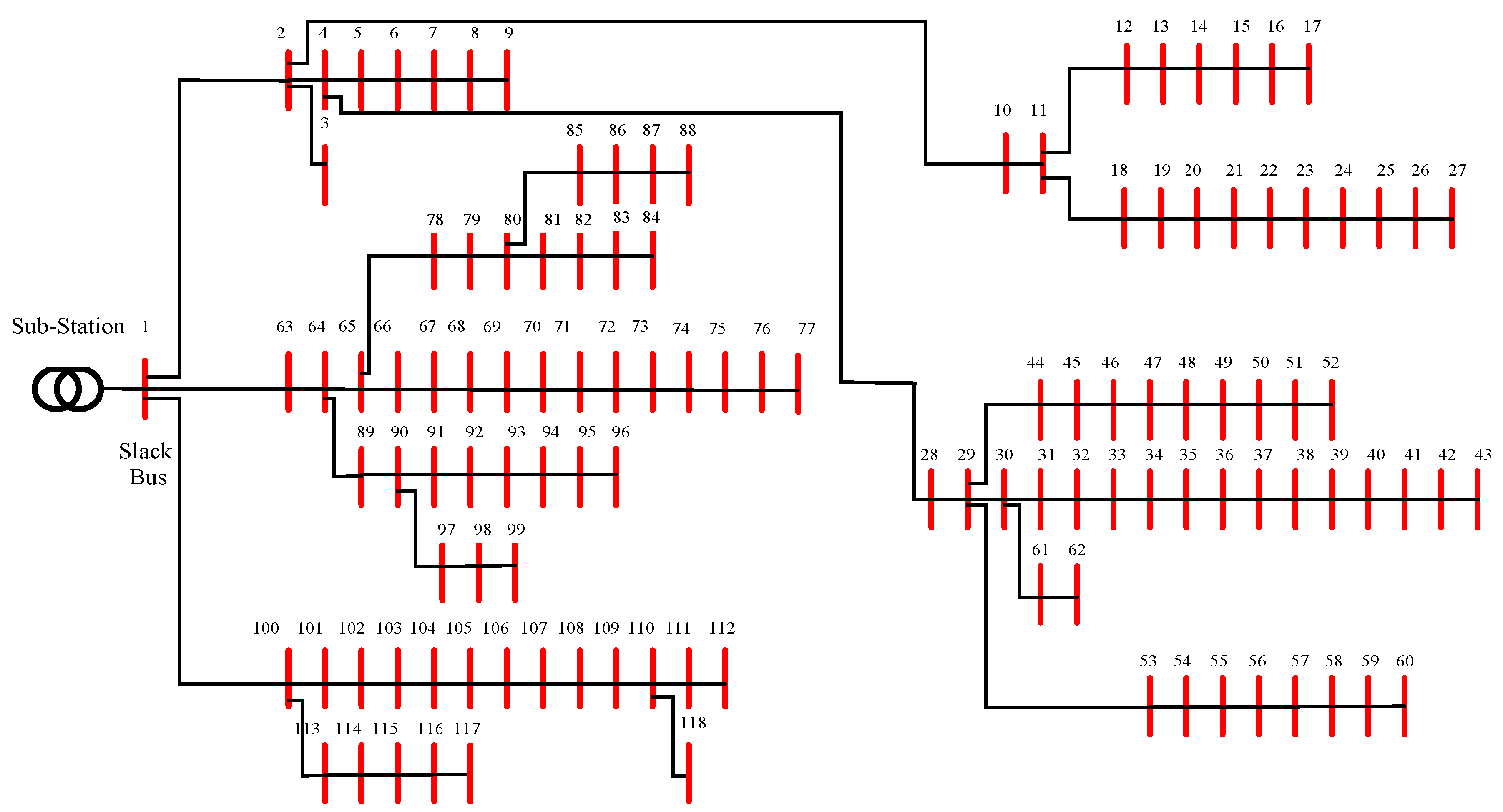
  • The optimal size and location of wind turbines, solar photovoltaics, and DSR resources are determined simultaneously under uncertainties to minimize costs, reduce voltage deviations, and improve voltage stability in the IEEE 118-bus DN.
  • The proposed I-WaOA is demonstrated to outperform other optimization algorithms, like SCSO, AHA, DO, HS, CDO, ZOA, ARO, and standard WaOA, in handling uncertainties and solving the complex optimal operation problem.

1.4. Organization of Article

The paper presents the structure of an optimal planning study of a power system under uncertainties. Section 2 introduces the problem and its mathematical formulation. Section 3 discusses the modeling of systems, while Section 4, Section 5 and Section 6 present the uncertainty parameters, mathematical formulations of the WaOA, and I-WaOA problems, respectively. Section 7 is reserved for simulation results and discussions, and Section 8 concludes the paper with the implications of the results.

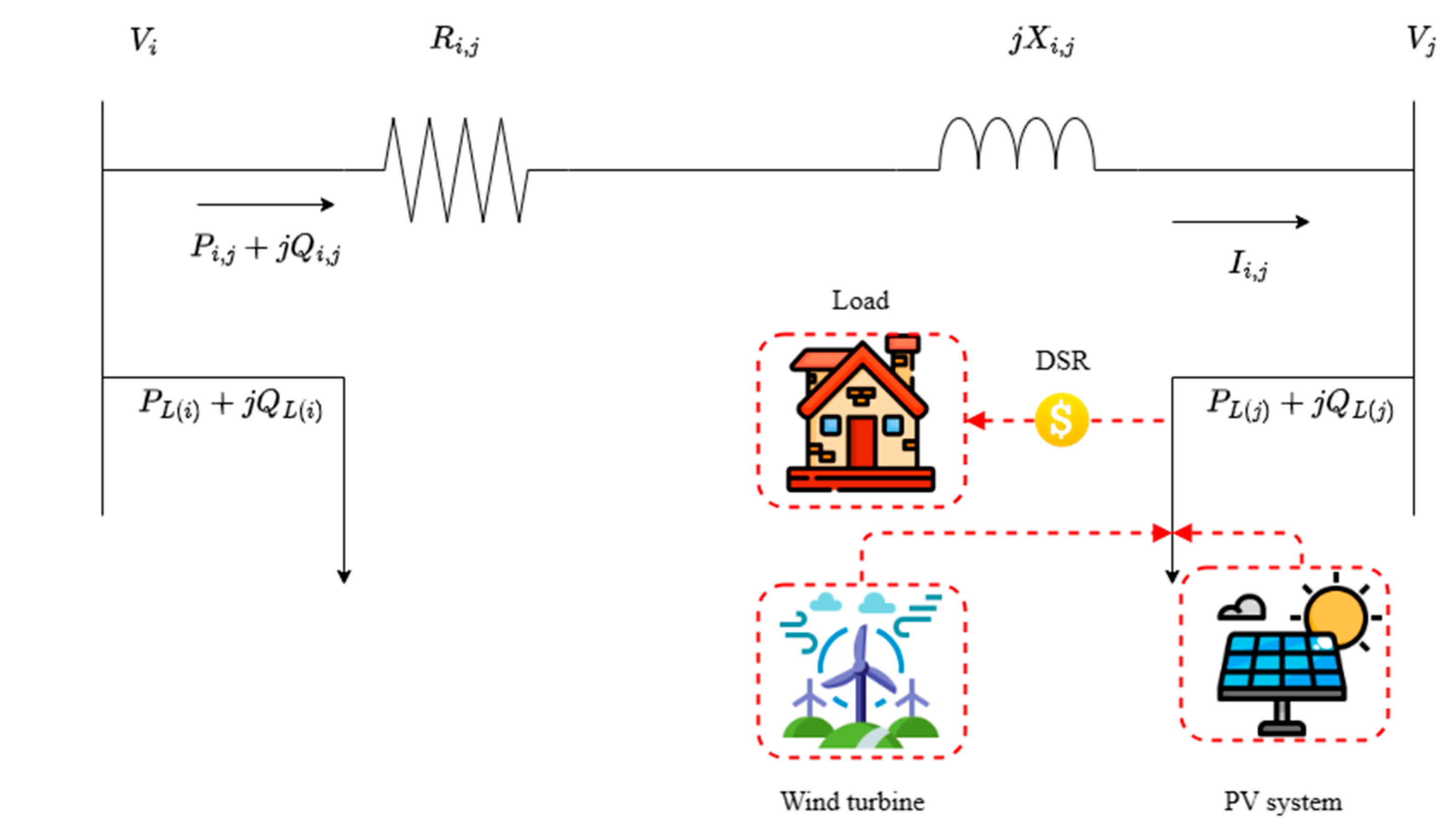
2. Formulating the Problem

This section presents the formulation of the problem, detailing both the optimal operation’s governing constraints and objective function.

2.1. Objective Function

Multiple objective functions are examined in this study, and they are as follows:

2.1.1. The Minimization of Costs

The considered objective function includes the cost of WT ( C W T ), the cost of PV units ( C P V ), the annual price of energy loss ( C L o s s ), and the price of electricity procured from the grid ( C G r i d ) . The total annual price can be written as:
C = C W T + C P V + C L o s s + C G r i d
In which,
C G r i d = 365 × h = 1 24 P G r i d ( h ) × U G r i d ( h )
where U G r i d is the price of buying energy from the network and P G r i d ( h ) is the hourly power taken out of the grid.
C L o s s = 365 × U L o s s × h = 1 24 P T _ L o s s ( h )
where U L o s s represents the expenditure associated with energy loss and P T _ L o s s ( h )   indicates the overall power losses during time h .
C P V = C P V i n s t + C P V O & M
where C P V O & M denotes the maintenance and operating expenses for the PV unit, while C P V i n s t represents the installation cost of the PV system.
C P V O & M = 365 × U P V O & M × i = 1 N s h = 1 24 P P V ( i , h )
C P V i n s t . = C F × U P V × P r a t e d _ P V
where P r a t e d _ P V is the maximum amount of power that the PV system can generate, and C F is a factor that influences how quickly the cost of the PV system is paid back.
C W T = C W T i n s t . + C W T O & M
where C W T O & M is the wind’s maintenance and operating costs and C W T i n s t . is the cost of installing the WT.
C W T O & M = 365 × U W T O & M × i = 1 N s h = 1 24 P W T ( i , h )
where the maintenance and operating expenses for WTs and PVs are represented by U W T O & M and U P V O & M . N s is the number of RESs with the DSR system considered.
      C W T i n s t . = C F × U W T × P r a t e d _ W T
where U W T and U P V stand for the corresponding purchasing costs of WTs and PVs. The rated generated power of WT is denoted by P r a t e d _ W T   . P W T ( i , h ) and P P V ( i , h ) denote the hourly produced power from WTs and PVs of the ith system.
C F = β × ( 1 + β ) N P   ( 1 + β ) N P 1
where N P and β are the system lifetime and interest rate of the PVs or WTs, respectively.

2.1.2. Increasing the Voltage Level

To ensure that the power grid operates efficiently and reliably, the voltage deviations should be maintained within an allowable range, ideally close to 1 p.u. The definition of the overall voltage deviation is [34,35]:
T V D = h = 1 24 i = 1 N B V ( i , h ) 1
where V ( i , h ) represents the hourly voltage of the ith bus and N B represents the number of buses in the network.

2.1.3. Enhanced System Stability

The index for voltage stability of the bus j is as follows [36,37]:
V S I j = V i 4 4   P j   X i , j Q j   R i , j 2 4 ( P j   R i , j + Q j   X i , j ) 2 V i 2
T V S I = h = 1 24 j = 2 N B V S I ( j , h )
where V S I ( j , h ) is the voltage stability index for bus j. P j and Q j define the real and reactive power flow of the branch between i and j near at bus j, respectively. X i , j and R i , j represents the reactance and resistance of the transmission line.
The optimization takes into account the following three goal functions concurrently:
min F = min ε 1 F 1 + ε 2 F 2 + ε 3 F 3
F 1 = C R E R s / D S R C B a s e
F 2 = T V D R E R s / D S R T V D B a s e
F 3 = 1 T V S I
where B a s e and R E R s / D S R are the base case and subscripts referring to RESs with DSR, respectively. The weighted values of ε 1 , ε 2 , and ε 3 were chosen to be 0.5, 0.25, and 0.25, respectively [15].

2.2. Inequality and Equality Constraints

2.2.1. Limitations of the Network (Inequality Constraints)

V m i n V ( i , h ) V m a x
i = 1 N s P P V _ r a t e d , i + i = 1 N s P W T _ r a t e d , i i = 1 N B P L o a d , i
P F m i n P F i P F m a x         i = 1,2 , , N s
I i I m a x , i                   i = 1,2 , , N T
where V max and V min are the upper and lower voltage limits, respectively. P Load represents the real load. N T defines the number of lines. I max , i is the maximum allowable current limit of the line i. P F min and P F max are the minimum and maximum of the WT power factor, respectively. The power factor of the PV farms should be equal to one.

2.2.2. Equality Constraints

P S ( h ) + i = 1 N s P P V , i ( h ) + i = 1 N s P W T , i ( h ) =   i = 1 N T P L o s s , i ( h ) + i = 1 N B P L o a d , i ( h )
Q S ( h ) + i = 1 N s Q W T , i ( h ) =   i = 1 N T Q L o s s , i ( h ) + i = 1 N B Q L o a d , i ( h )
where Q S ( h ) and P S ( h )   are the hourly reactive and real powers of the main network, respectively.

3. Modeling the Systems
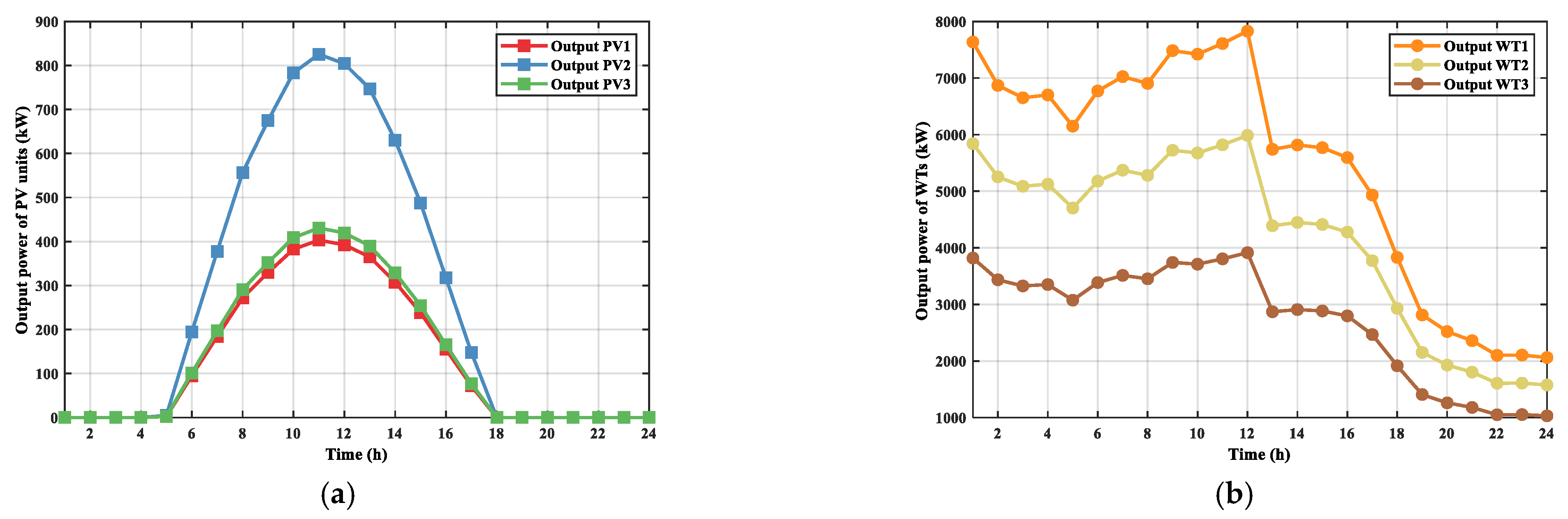
3.1. PV System

The power output of a PV system can be determined using the following formula:
T c ( h ) = T a ( h ) + I h 800 N O C T 20
P P V h = A P V η P V h I h
The total area used by the PV array, labeled as A P V in (m2), is multiplied by a number representing the efficiency of conversion of the PV panels, η P V , to get the output produced by the PV, expressed as P P V (kW). The temperature of the cell is expressed in degrees Celsius as T c . The temperature outside in degrees Celsius is represented by T a . I is the solar insolation in (kW/m2). The instantaneous efficiency of PV panels η P V is obtained using the following equation [38]:
η P V ( h ) = η r η t × 1 γ T a h T r γ I ( h ) N O C T 20 800 1 η r η t
where η t is the effectiveness of the maximum power point tracking device, and η r is the PV panels’ reference efficiency. It also takes into account the temperature coefficient of efficiency γ , which for silicon cells, normally ranges from 0.004 to 0.006 per (°C). Notable operating cell temperature N O C T in (°C), reference temperature T r in (°C) for PV cells, and ambient temperature T a in (°C) are also considered.

3.2. WT System

The WT energy output ( P W T ) can be determined using the following formula:
P W T W = 0 f o r W < W i   a n d   W > W o P r a t e d _ W T W W i W r W i f o r W i W W r P r a t e d _ W T f o r   W r < W W o
The used wind turbine has a rated power of 250 kW, a rated velocity W r of 15 m/s, a cut-out speed W o of 25 m/s, and a cut-in speed W i of 2.5 m/s [39].

3.3. Demand Side Response

The power fluctuations in the distribution system can vary significantly on a daily basis, resulting in substantial differences between the minimum and maximum energy consumption. Demand Side Response is a viable approach to modifying customers’ consumption patterns. In essence, DSR entails altering the power consumption of electric utility customers to align it more effectively with the system’s supply. In other words, demand response programs focus on adjusting the demand for power rather than manipulating the supply [40,41].
In this research, the real-time pricing (RTP) program is employed as the demand-side response program due to its widespread and practical application. RTP is considered one of the most common and beneficial DSR programs, and its implementation in a real distribution system is relatively straightforward. As a result, the outcomes of this study closely align with the performance of an actual distribution system [42,43].

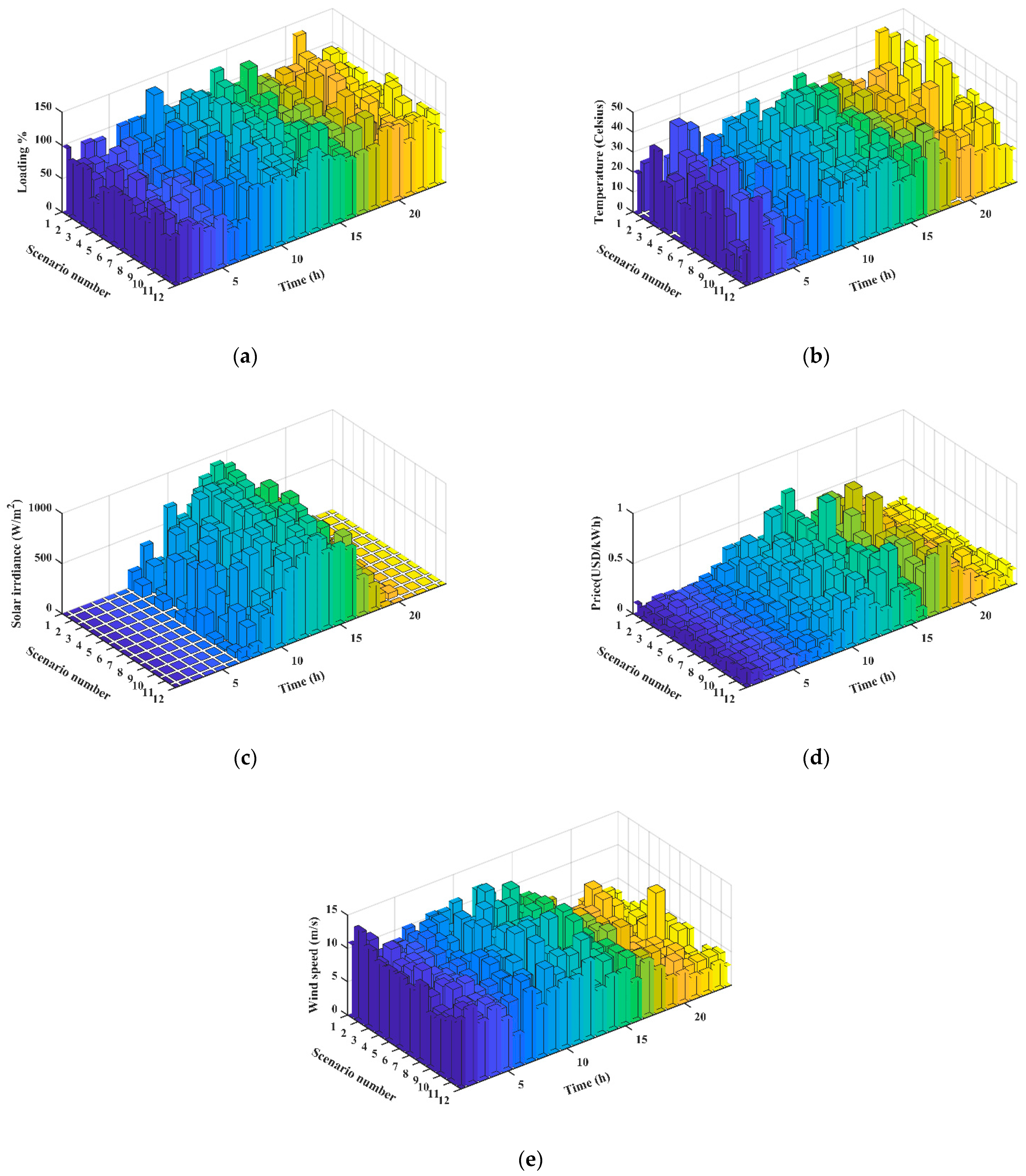
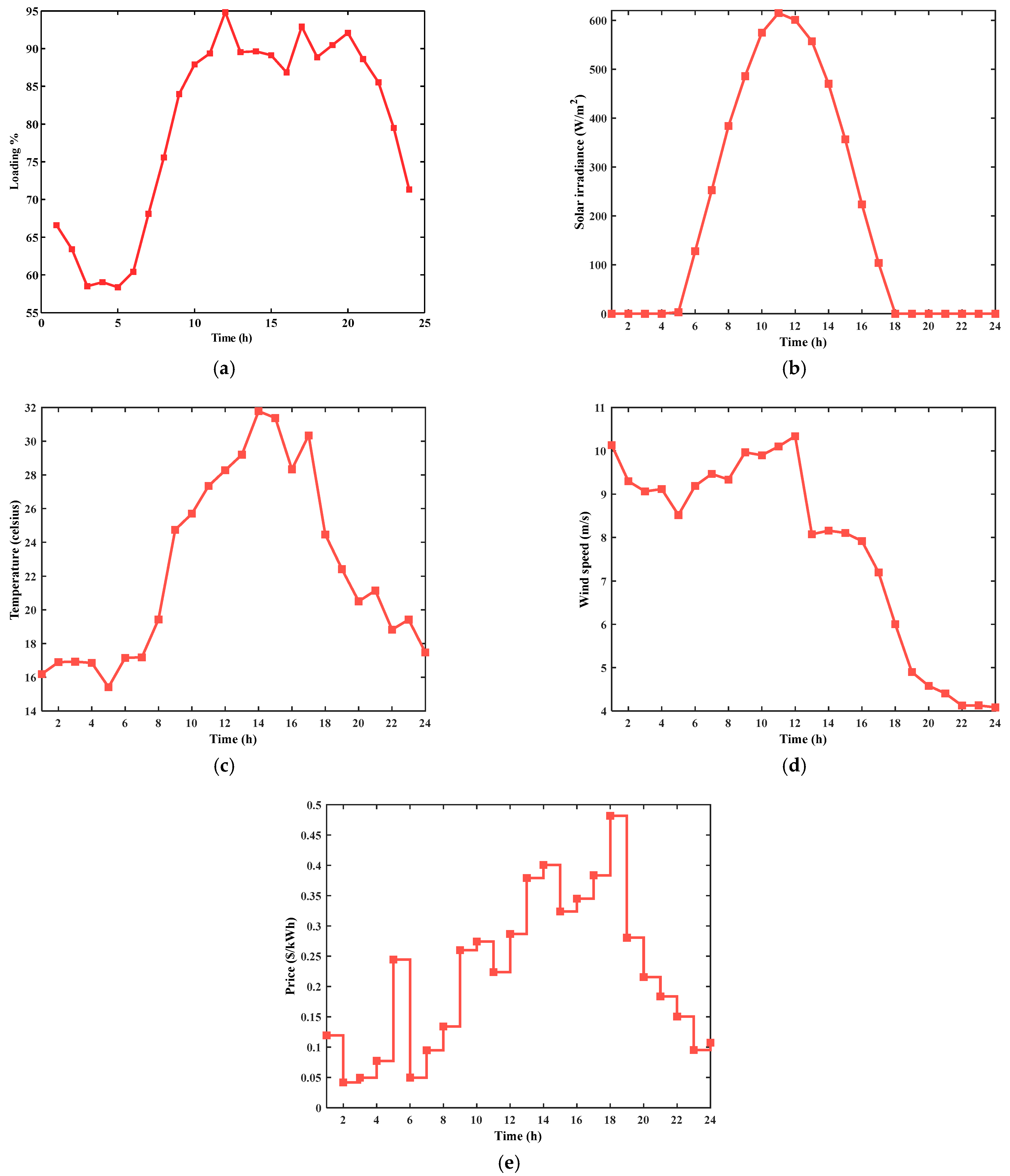
4. Representing the Uncertainties

The uncertainty in the parameters is depicted in the following manner:

4.1. A Probabilistic Representation of Solar Irradiance

The variations in sun irradiance have been modeled using the Beta PDF in the following way [44,45]:
f b ( G ) = Γ φ + τ Γ φ Γ τ s φ 1 ( 1 G ) τ 1 0 G 1 ; φ , τ 0 0 otherwise
where μ represents the mean value derived from past data and σ is the standard deviation. The following equations can be used to determine τ and φ [46,47]:
τ = 1 μ × μ × 1 + μ σ 2 1
φ = μ × τ 1 μ

4.2. A Probabilistic Representation of Wind Speed

To represent the uncertainty of wind speed, the following is an explanation of how the Weibull PDF is applied [48,49]:
F ( W ) = k c W c k 1 e x p W c k
where W stands for the speed of the wind. The Weibull PDF scale and parameters for shape are represented by the c and k , respectively.

4.3. A Probabilistic Representation of Load Demand

The normal PDF can be used to model the uncertainty in load demand as follows. [47]:
f n L = 1 σ L 2 π × e x p L μ L 2 2 σ L 2
where the loading’s mean value is represented by μ L and the standard deviation is represented by σ L .

4.4. The Probabilistic Representation of Price

The price of electricity is a highly important random characteristic in a power system since it is an uncertain value derived from the grid. Equation (33) illustrates how the normal PDF, based on its mean value μ P and standard deviation σ P , can be used to simulate the PDF of the price of electricity [50,51]:
f P = 1 σ P 2 π e x p P μ P 2 2 σ P 2

4.5. The Probabilistic Representation of Temperature

Since the temperature outside is constantly changing, it is considered an erratic variable, and its uncertainty is expressed as follows using the normal probability distribution:
f T = 1 σ T 2 π e x p ( T μ T   ) 2 2 σ T 2
where the mean temperature is represented by μ T and the standard deviation by σ T .
Monte Carlo simulations were used to generate 800 data points for solar irradiance, temperature, wind speed, load, and price, using the parameters of the probability density function (PDF) of each variable determined from the collected data [52]. However, to reduce the computational burden of the simulation, a data-based reduction method followed by conditional control was used to reduce the number of cases to a more manageable size (12 cases) [53,54]. Figure 2 shows generated scenarios of these parameters at 12:00. A.M.
Figure 3 illustrates specific scenarios selected for Monte Carlo simulations of a power system over a 24 h period after data reduction. The figure provides a unique insight into the probabilistic analysis of the system, where the data have been refined to enhance simulation efficiency and present an accurate depiction of potential scenarios throughout the specified period.

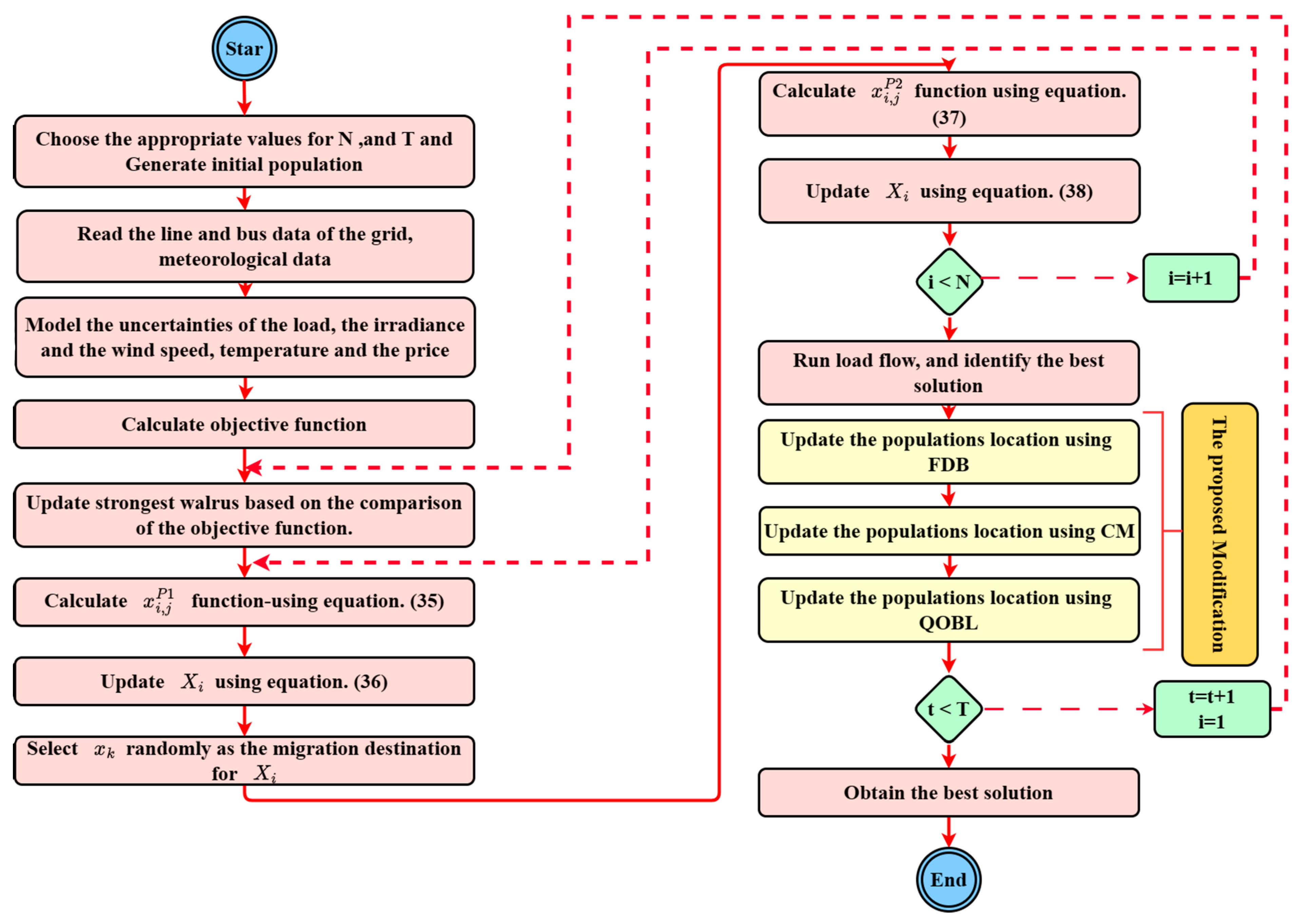
5. Walrus Optimization Algorithm (WaOA)

WaOA is a bio-inspired algorithm that uses the behavior of walruses to search for food. By randomly initializing the population of walruses and then moving them around according to their fitness values, WaOA can effectively explore the search space and find better solutions [55].

5.1. Feeding Strategy

The position of each walrus is updated by moving towards the strongest walrus, which is the best solution found so far. The mathematical representation of updating the walruses’ positions is structured around their feeding behavior, guided by the dominant member of the group, as described by Equations (35) and (36).
x i , j P 1 = x i , j + r a n d i , j S W j I i , j x i , j
X i = X i P 1 , F i P 1 < F i , X i ,   else ,  
In the first phase of WaOA, new positions x i , j P 1 for each walrus   i t h are generated based on the feeding strategy. The   j t h dimension of the new position is x i , j P 1 . After evaluating the function of objective F i P 1 at this new location,   x i , j   represents the location of particle i in dimension j. Meanwhile, X i   is a vector that encompasses the position across all dimensions. rand i , j introduces randomness by generating numbers between 0 and 1. The best solution so far S W j acts as the strongest walrus that guides movement. To boost exploration, I i , j are integers of 1 or 2 chosen randomly. I i , j   = 2 causes broader jumps versus 1 for normal steps. This expands the search space, helping to escape local optima and find new promising areas. In summary, the first phase updates positions via a randomized process biased towards the best solution so far. Occasional large steps enhance global exploration to avoid getting trapped.

5.2. Migration

The position of each walrus is updated by migrating toward the position of another randomly selected walrus. WaOA utilizes this migration procedure to steer the walruses throughout the exploration of the search space, aiding them in identifying favorable regions within it. This behavioral mechanism is formally expressed through Equations (37) and (38).
x i , j P 2 = x i , j + r a n d i , j x k , j I i , j x i , j , F k < F i , x i , j + r a n d i , j x i , j x k , j , e l s e ,
X i = X i P 2 , F i P 2 < F i , X i ,   else ,  
Here,   x i , j P 2 represents the newly generated position of the   i t h walrus derived from the second phase. x i , j P 2 signifies its position on the jth dimension. F i P 2 corresponds to its objective function value. X k , where k     { 1 ,   2 ,   ,   N } and k     i , represents the position of the selected walrus to which the ith walrus is migrated. x k , j is the position of the k t h walrus on the jth dimension, and F k indicates its objective function value.

5.3. Escaping Predators

WaOA uses the natural behavior of walruses to improve its ability to find food. By simulating the way walruses shift their positions in response to threats, WaOA can more effectively explore the search space and find better solutions. In the algorithm, a virtual neighborhood is established around each walrus, where new positions are randomly generated within this range using Equations (39) and (40). If the objective function improves with this novel location, it substitutes the old one, as outlined in Equation (41). This behavior simulation within WaOA enhances its efficacy in local search and adaptation to the problem’s landscape.
x i , j P 3 = x i , j + l b l o c a l , j t + u b l o c a l , j t   rand   l b l o c a l , j t
Local   bounds   :   l b l o c a l , j t = l b j t , u b l o c a l , j t = u b j t ,
X i = X i P 3 , F i P 3 < F i , X i ,   else ,  
In this context, x i , j P 3   refers to the newly created position of the   i t h walrus using the third phase. x i , j P 3 designates its location on the   j t h dimension. F i P 3   stands for its objective function value. t represents the iteration cycle. l b j and u b j   symbolize the lower and upper limits of the   j t h variable, respectively. Additionally, l b l o c a l , j t   and u b l o c a l , j t   denote the locally permitted lower and upper bounds for the   j t h variable, respectively, which simulate localized exploration within the vicinity of potential solutions.

6. Improved Walrus Optimization Algorithm (I-WaOA)

I-WaOA employs three strategies. The initial approach uses the Cauchy mutation, followed by the second method grounded in the fitness-distance balance (FDB) concept. The final strategy is the Quasi-Oppositional-Based Learning (QOBL) method.

6.1. The Cauchy Mutation (CM)

CM is a powerful technique that can be used to improve the efficiency of algorithm optimization. It has been shown to be effective in escaping from local optima and finding better solutions to problems [29,56,57]. In the proposed algorithm, CM is used to generate new solutions that are more likely to be better than the current solutions. The mathematical representation of CM is as follows:
X i t + 1 = X i t + α   Cauchy   ( μ , σ ) X i t X best  
F ( x ) = 1 π a r c t a n 2 ( x μ ) σ + 1 2
where represent entrywise multiplication, α denotes to the step size, Cauchy   ( μ , σ ) represent Cauchy distribution with mean μ and standard deviation σ , F ( x ) is cumulative distribution function of the Cauchy distribution function, and σ and μ are the scale parameters and the location, with values selected to be 4.5 and 0.8, respectively [58].

6.2. The Fitness-Distance Balance (FDB)

One way to choose the ideal optimization solution from the pool of available options is to use the FDB selection method. It works by measuring the value of the strength of each candidate solution and its distance from the optimal solution. The difference between two solutions is calculated by taking the absolute value. The FDB method then selects candidate solutions with their highest fitness values and shortest distances to the optimal solution. This helps the algorithm focus on candidate solutions that are good and search the search area around the optimal solution [59,60,61,62].
D S i = x i 1   Best   1 2 + x i 2   Best   2 2 + + x i d   Best   d 2
Then, build the fitness and distance value vectors in the following manner:
D S = D S 1 , D S 2 , , D S n
F = F 1 , F 2 , , F n
After that, the fitness and distance values may be adjusted in the manner shown below:
n o r m D S i = D S i m i n ( D S ) m a x ( D S ) m i n ( D S )
n o r m F i = F i m i n ( F ) m a x ( F ) m i n ( F )
where the fitness vectors and distance’s minimum and maximum are represented by the terms m i n and m a x , respectively. The FDB score is determined using the formula below:
FDB score   i = α 1 n o r m F i + ( 1 α ) n o r m D S i
In which
α = 0.5 1 + t T m a x

6.3. The Quasi-Opposite Based Learning (QOBL)

QOBL is a highly effective method designed to identify specific regions within a population that are likely to yield optimal solutions. By strategically employing the QOBL selection and promptly assigning it a collision count, the algorithm expedites the process, leading to improved efficiency in the context of meta-heuristic algorithms [63,64,65,66,67,68]. The following is an illustration of QOBL.
f o r   i = 1 : N o . Populations
   f o r   j = 1 : N o . Dimensions
     x i , j o = L b j + U b j x i , j
     C i , j = L b j + U b j / 2
     i f   ( x i , j < C i , j )
       x i , j q o = C i , j + x i , j o C i , j ×   rand
       e l s e
         x i , j q o = C i , j + C i , j x i , j o ×   rand
     e n d
   e n d
e n d
The Improved Walrus Optimization Algorithm represents an enhanced iteration of the WaOA algorithm, integrating three key strategies to elevate its performance. The utilization of Cauchy mutation, a more assertive operator than in the original WaOA, enables I-WaOA to break free from local optima, fostering exploration across new regions of the search space. The incorporation of Fitness-Distance Balance ensures a harmonized equilibrium between exploration and exploitation capabilities, preventing entrapment in local optima and facilitating the discovery of the global optimal solution. Additionally, the Quasi-Oppositional-Based Learning method empowers I-WaOA to navigate uncharted territories within the search space, contributing to its proficiency in locating the global optimal solution. The I-WaOA algorithm was developed to examine the weaknesses of the basic WaOA algorithm, such as its susceptibility to getting trapped in local optima and its potential for performance improvement.
The I-WaOA for the optimal operation solution is shown in Figure 4. Figure 5 shows the process for solving the stochastic OOP of a DN.

7. Results of Simulation

The performance of the proposed Improved Walrus Optimization Algorithm (I-WaOA) for solving the IEEE 118-bus system optimization problem was evaluated by comparing it against several established optimization algorithms. These included Chernobyl disaster optimizer (CDO) [69], Artificial hummingbird algorithm (AHA) [70], Dandelion Optimizer (DO) [71], Harmony Search (HS) [72], Artificial rabbits optimization (ARO) [73], Sand Cat swarm optimization (SCSO) [74], Zebra optimization algorithm (ZOA) [75], and standard walruses behavior (WaOA) [55]. All the algorithms were executed using MATLAB R2019b on a computer with 6 GB of RAM and an Intel i7 CPU running at 2.5 GHz. The comparative analysis aimed to assess the performance of the proposed I-WaOA against current state-of-the-art optimization techniques. The different cases that were studied are presented here:

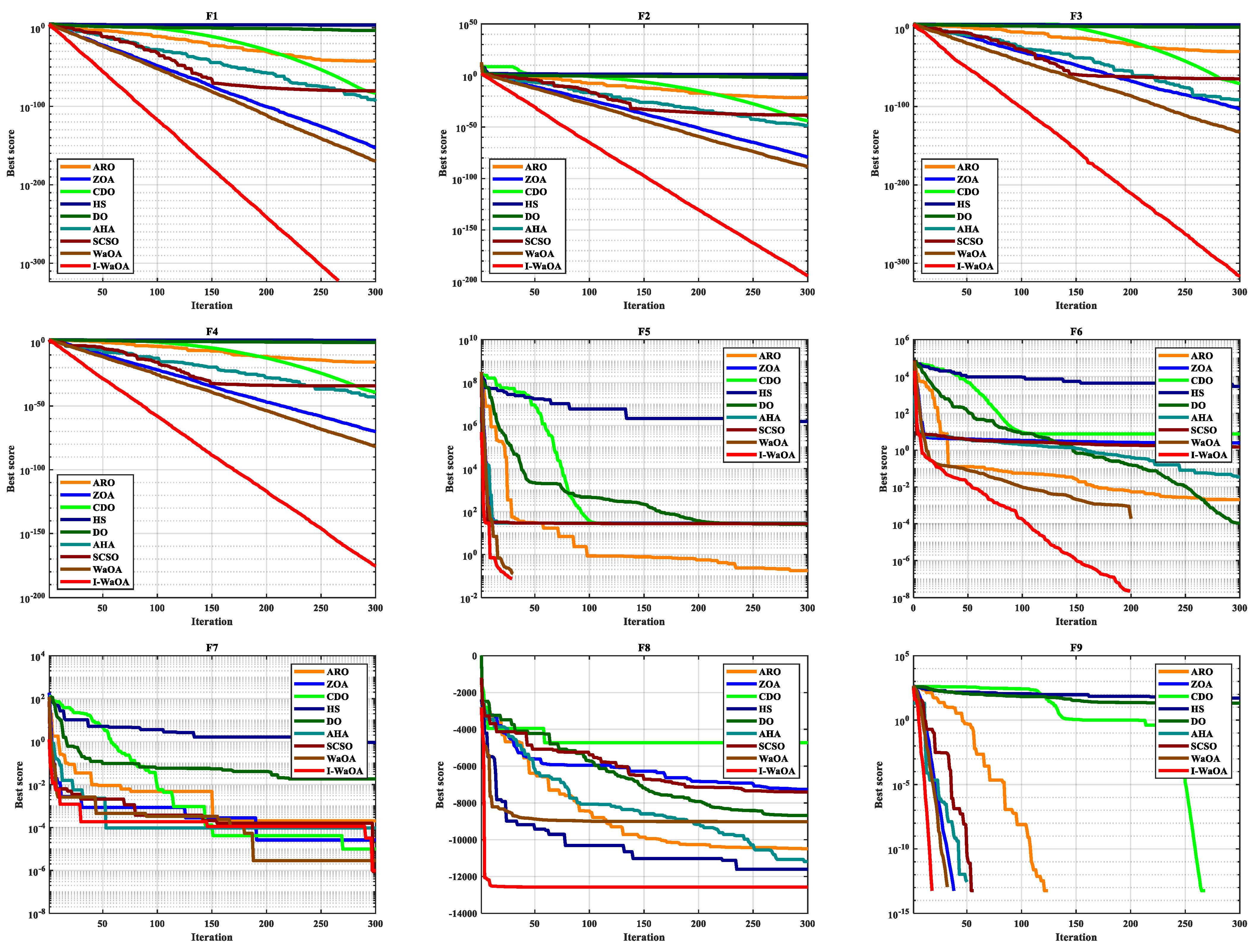
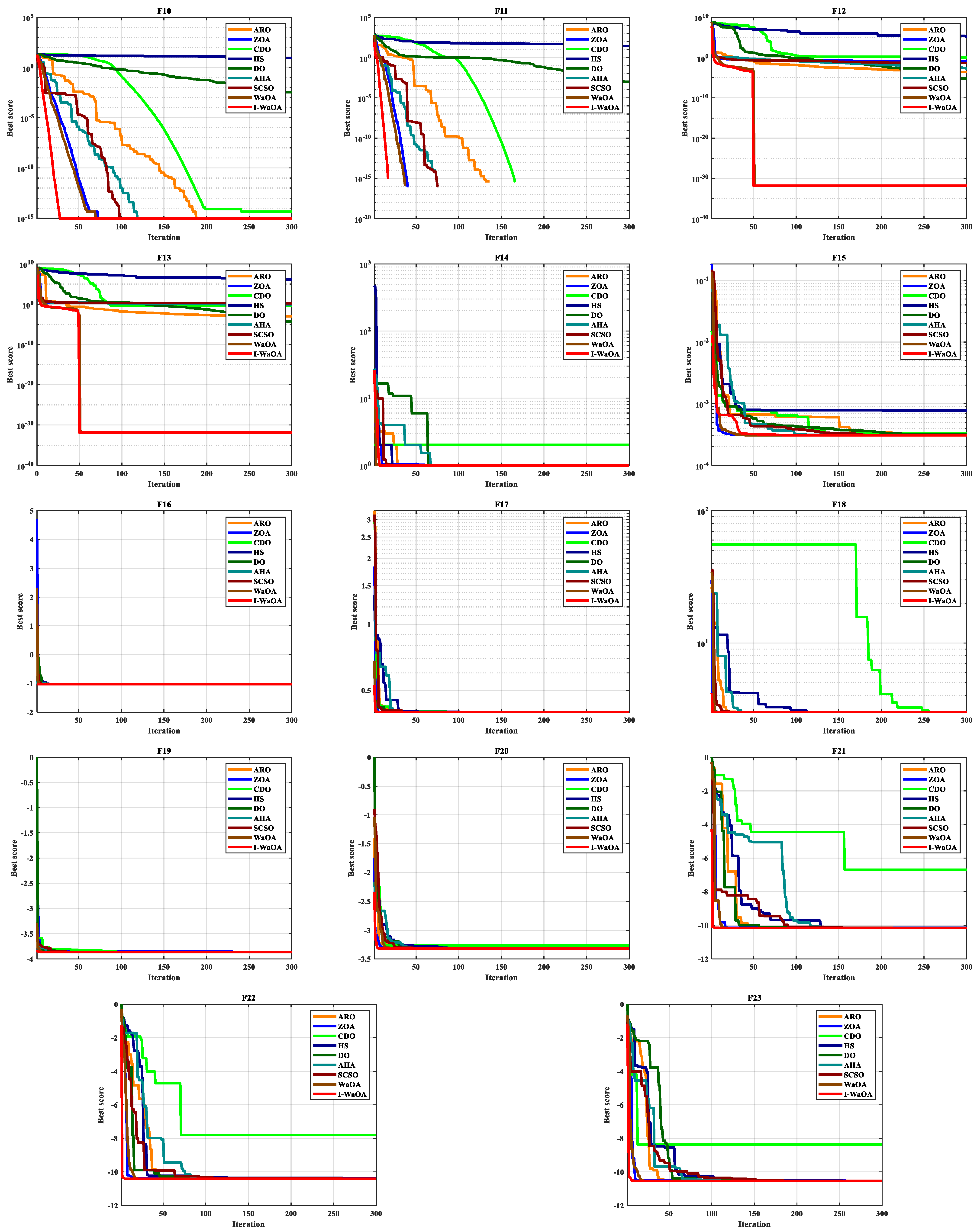
7.1. Testing the I-WaOA Technique on a Set of Commonly Used Test Functions

In this study, we employ the proposed I-WaOA method to evaluate 23 classic functions shown in Table 2, Table 3 and Table 4 [76,77,78]. To ensure consistency, the parameters for all situations are set based on Table 5, and the results are recorded after running the experiment 30 times.

7.1.1. Statistical Results Analysis

This section presents a comparative analysis of the proposed I-WaOA with other optimization methods, including SCSO, AHA, DO, HS, CDO, ZOA, ARO, and the conventional WaOA. Statistical results, as shown in Table 6, encompass the mean, worst, SD, and best among all algorithm approaches.
Table 6 shows that for the majority of the functions under study, the suggested I-WaOA optimizer performs better than the others in terms of worst, best, and mean values. This means that the I-WaOA optimizer was able to find better solutions on average, as well as the best and worst solutions, than the other optimizers. All algorithms have a community size of 30 and a maximum iteration of 300.

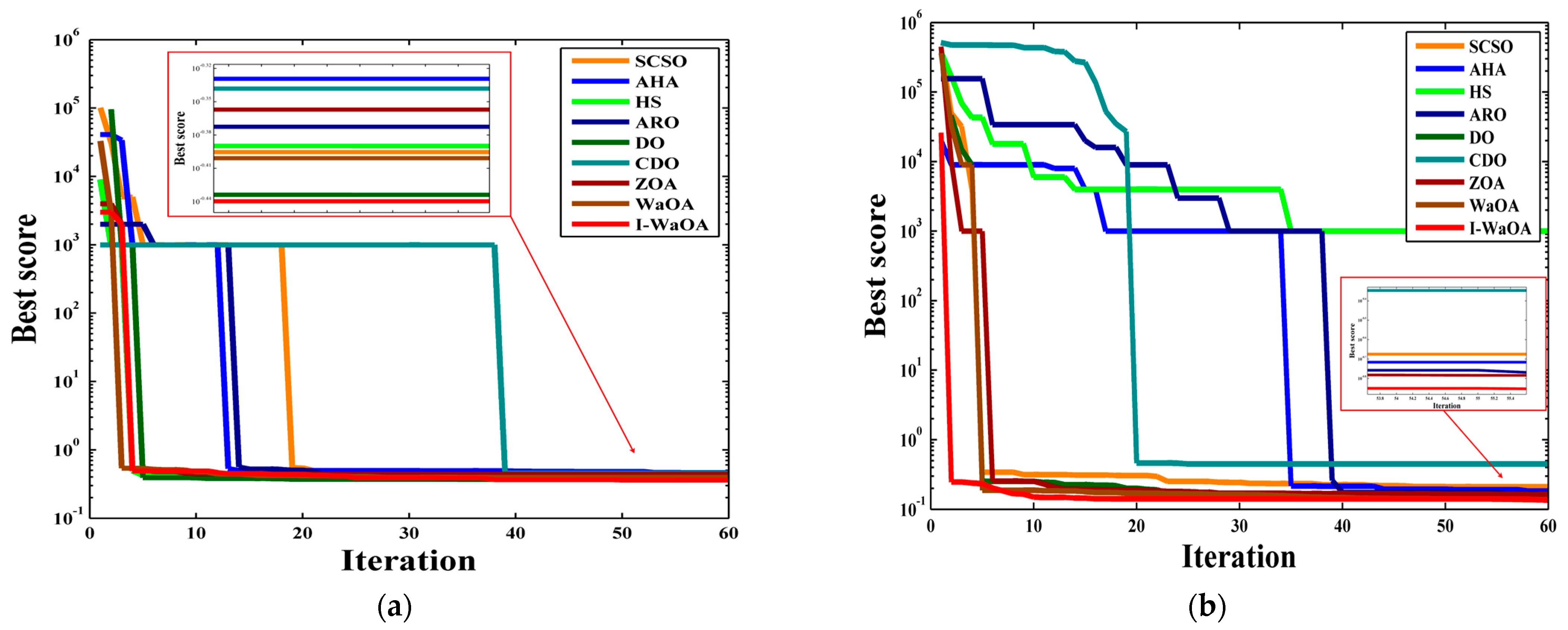
7.1.2. Convergence Curve Analysis

The I-WaOA algorithm’s convergence graphs and those of other previously published techniques, including AHA, SCSO, DO, HS, CDO, ZOA, ARO, and standard WaOA, can be observed in Figure 6.
The proposed I-WaOA algorithm was shown to be more accurate and faster than other algorithms based on convergence curves. The proposed modifications to the WaOA algorithm enhance both the exploration and exploitation phases of the algorithm, which allows it to converge to an optimal solution more quickly than the traditional WaOA algorithm.

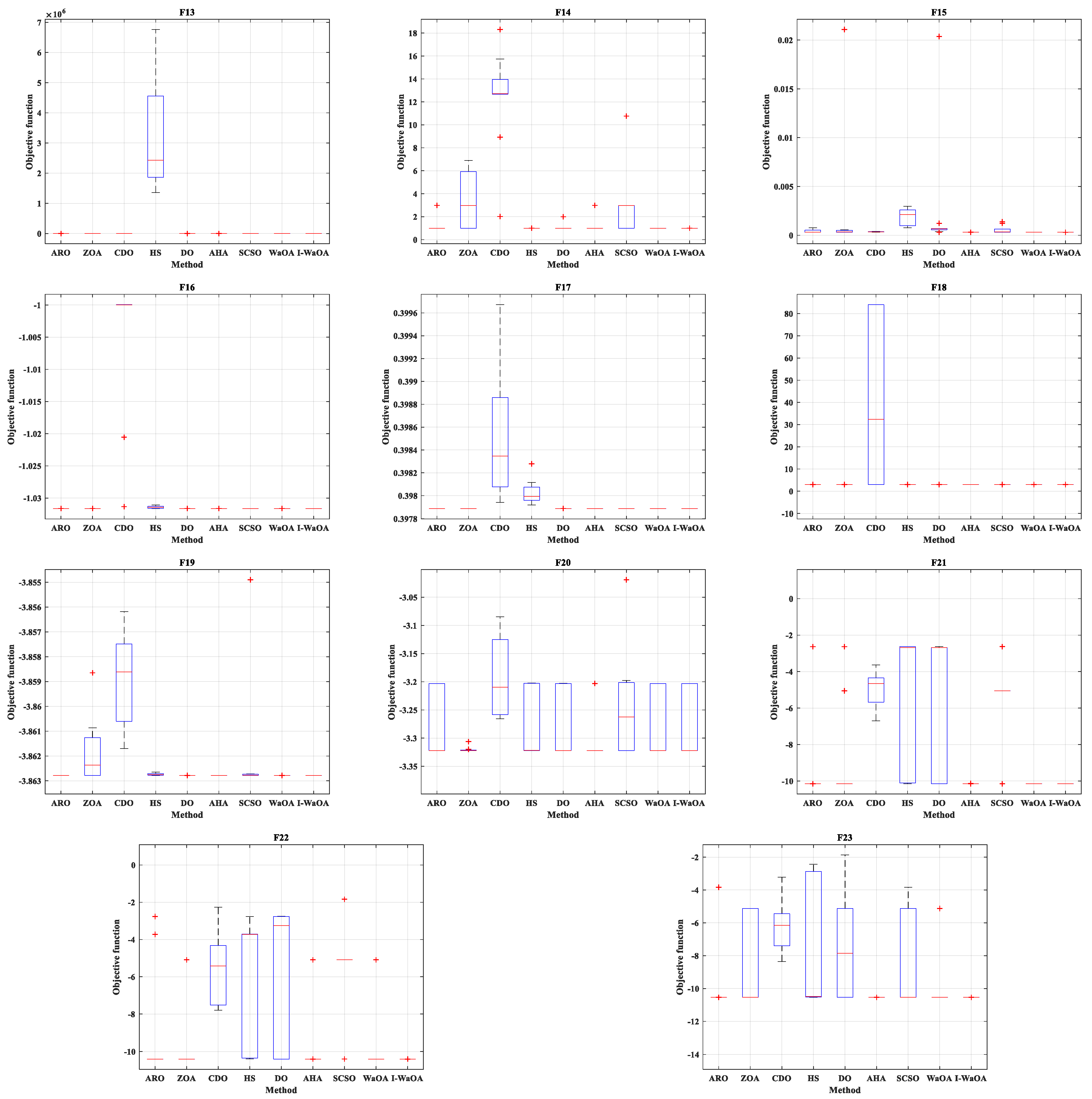
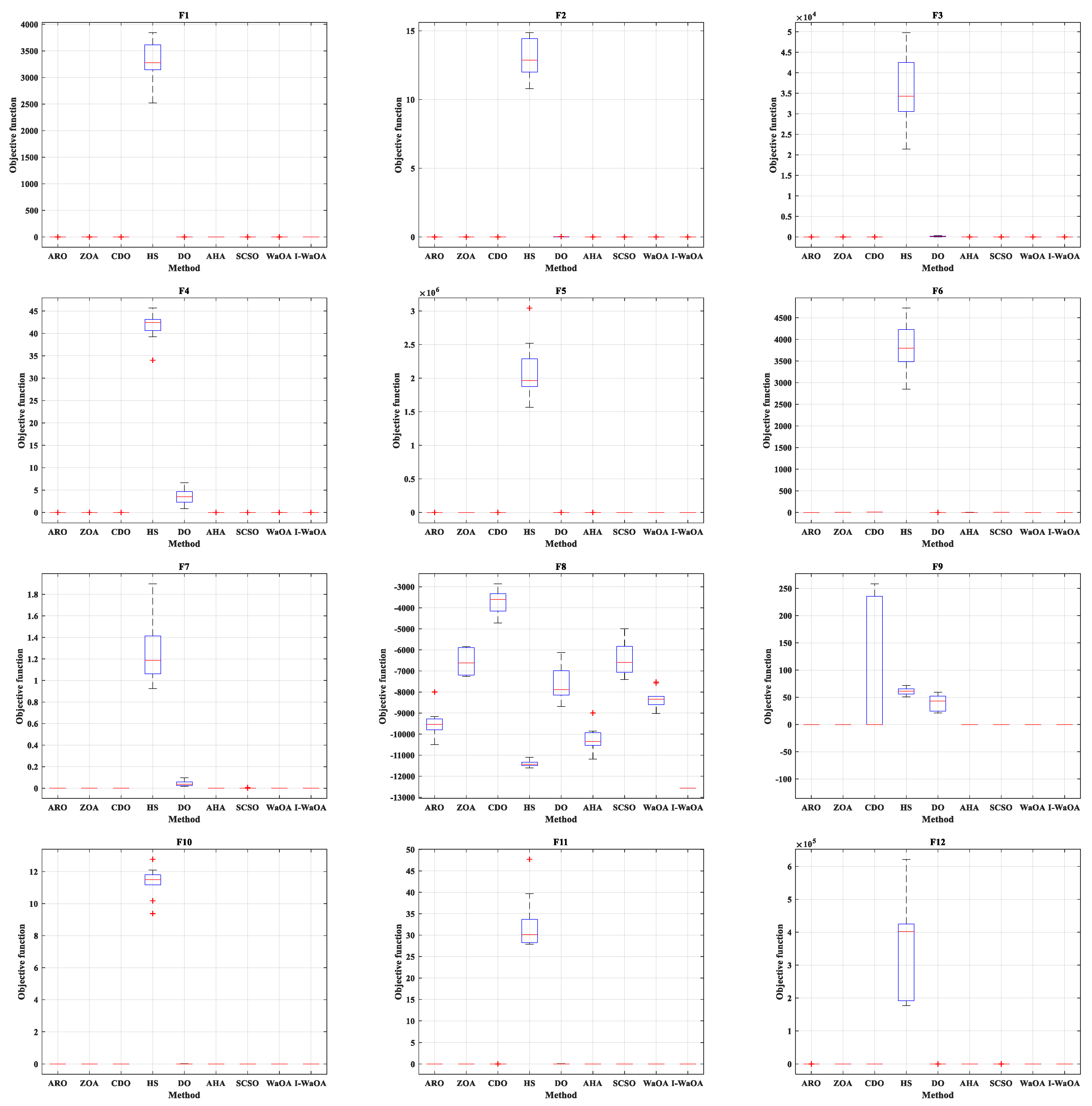
7.1.3. Analysis Using Boxplots

Boxplot graphs effectively display data distribution patterns in four equal groups, enabling examination of data distribution features. Figure 7 shows the boxplots for the proposed I-WaOA method and other published optimization techniques. The boxplots for I-WaOA visibly display a smaller spread compared to the other optimization techniques.

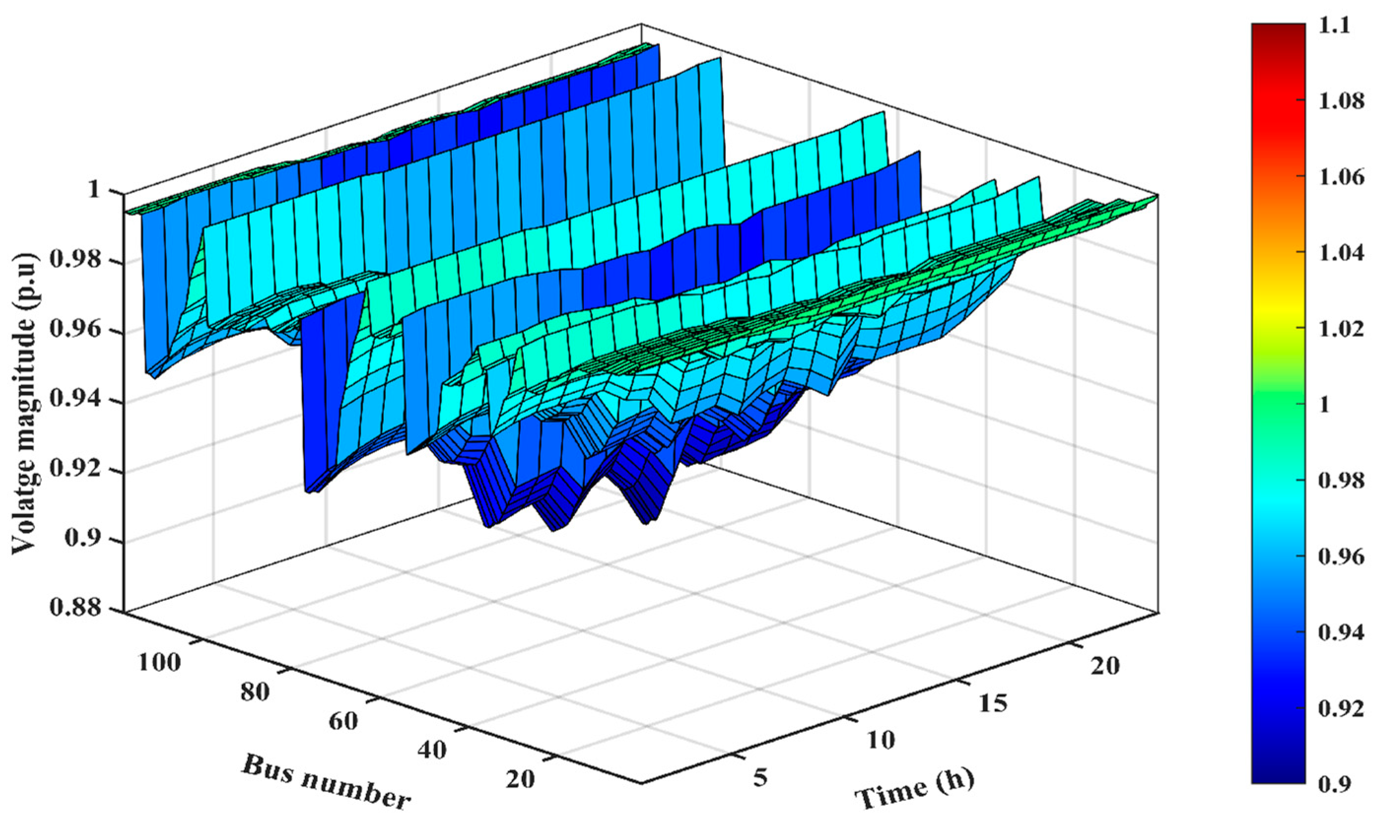
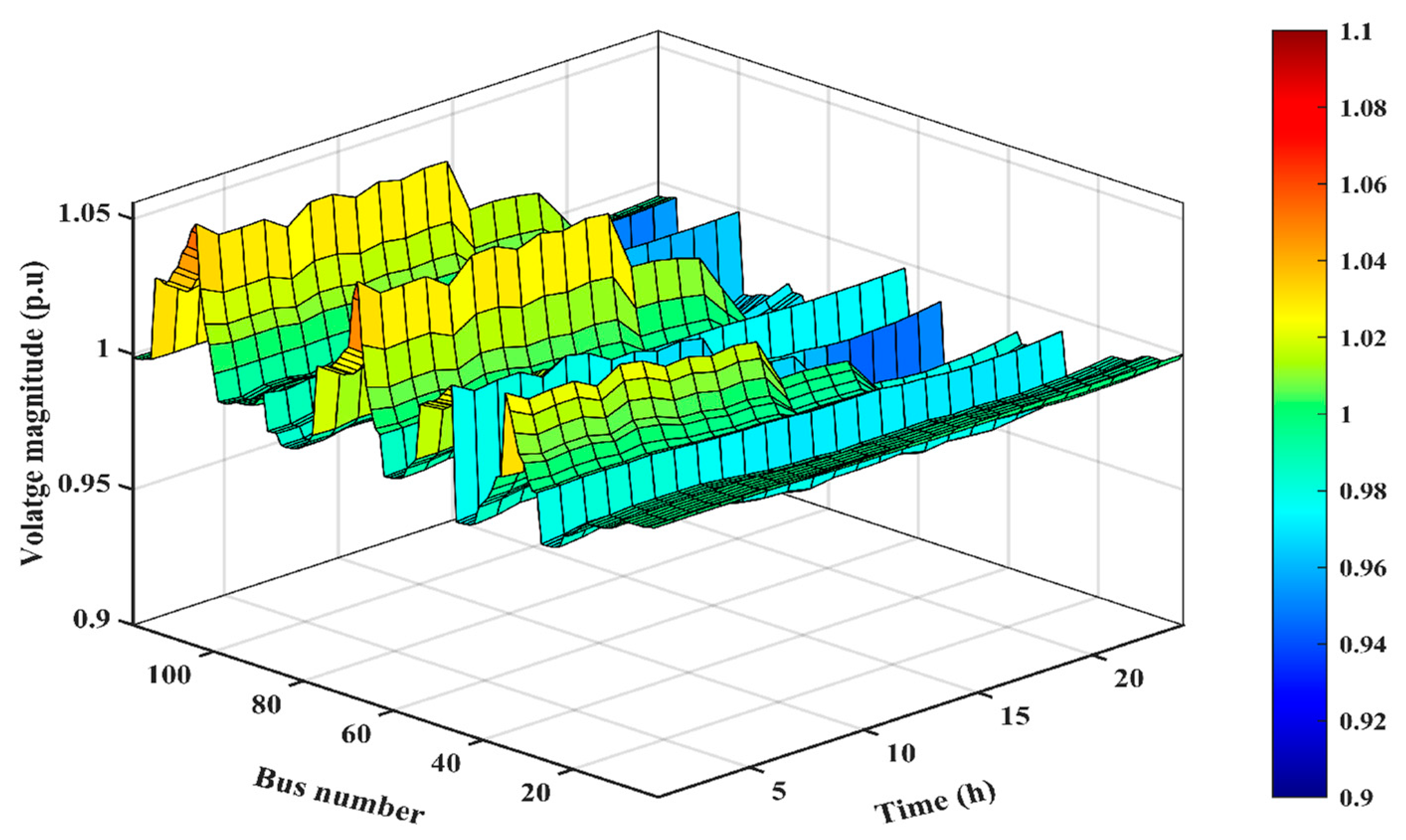
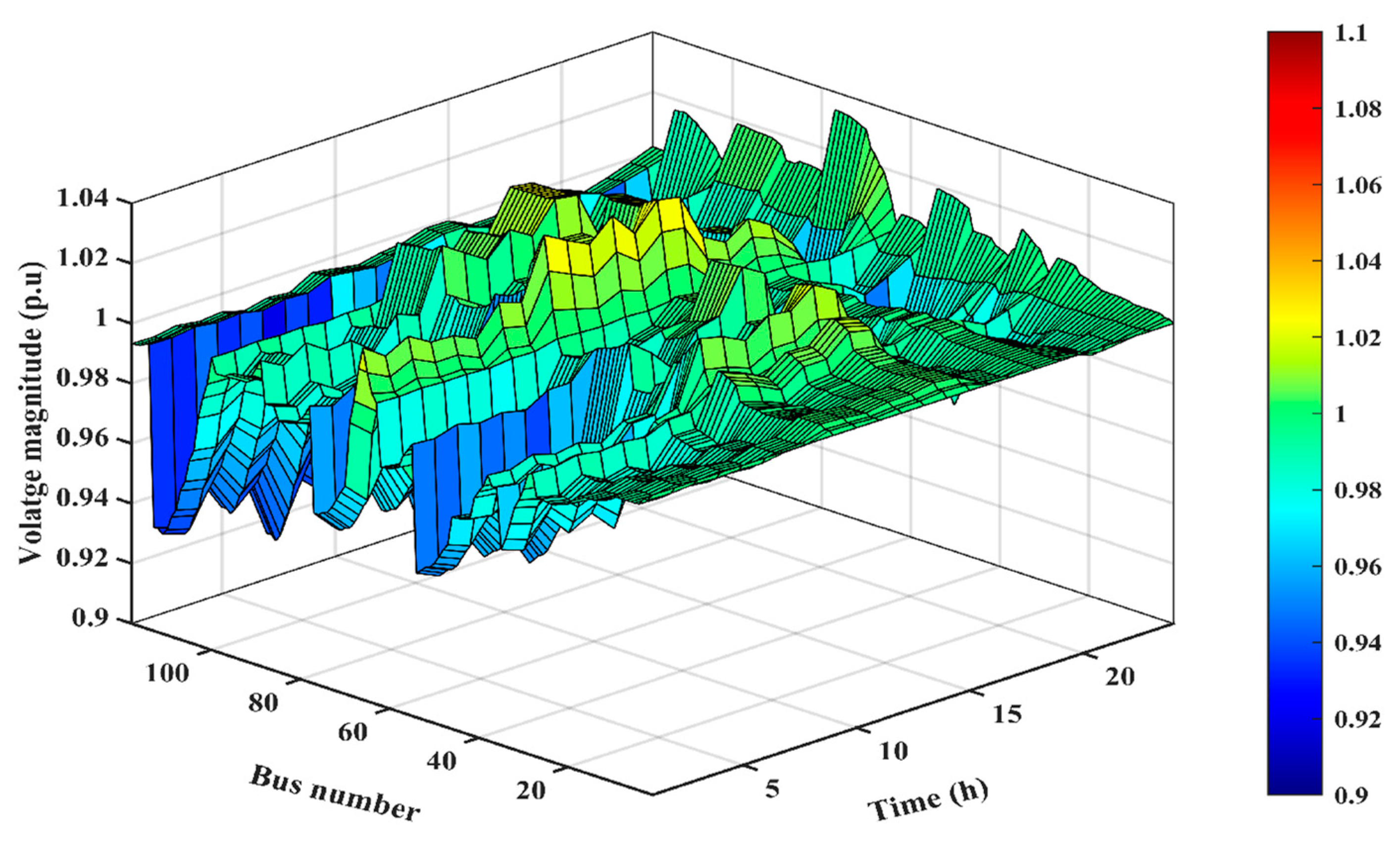
7.2. Applying the Suggested Approach to Solve the IEEE 118 Distribution Network’s Optimal Operating Problem

In this section, we implement the I-WaOA approach to address the OOP and ascertain the optimal placement of three systems composed of one PV unit rating and one WT in each system within the IEEE 118 distribution network. The configuration, depicted in Figure 8, encompasses 118 buses and 117 branches. Pertinent data are provided in [79]. Meteorological information, including wind speed and solar radiation, along with temperature data, is sourced from [7,80], respectively. To verify the suggested I-WaOA algorithm’s effectiveness, we conduct a comparative analysis between its results and those obtained from the original method. For a meaningful and unbiased comparison, the population size and maximum iteration count of the suggested methods are fixed at 25 and 60, respectively. Table 7 lists the operational restrictions together with the RESs price variables.
The methodology presented in Section 4 took into account a variety of uncertainties, encompassing variations in electricity price, wind speed, temperature, solar irradiation, and load. Figure 9 shows the anticipated day-ahead load demand, market energy purchasing prices, wind speed, irradiance, and temperature patterns.
The results obtained from conducting case studies on the 118 bus system are presented in Table 8. This table provides information about the impact of integrating PVs and WTs both with and without Demand Side Response on the system. Overall, it offers insights into how PVs, WTs, and DSR can enhance the operation of distribution grids that utilize energy sources.
The primary goal of this study was to optimize expenses while enhancing the performance of the system by incorporating renewable energy resources and Demand Side Response into an electrical DN. The findings indicated that the proposed I-WaOA algorithm proved effective in reducing costs, improving voltage stability, and minimizing voltage deviations. In the scenario where no RESs were integrated into the DN, the total annual cost amounted to 3.8806 × 10⁷ USD. However, by using the suggested I-WaOA algorithm and strategically allocating RES, this cost is significantly decreased to 1.8230 × 10⁷ USD, resulting in a reduction in voltage deviations from 98.6633 per unit (p.u.) to 49.9790 p.u. Moreover, there was an enhancement in Voltage Stability Index, increasing from 2.4440 × 10³ p.u. to 2.6965 × 10³ p.u. The best places for the systems in the DN are 35, 68, and 104, respectively. The WTs ratings are 4250 kW, 6500 kW, and 8500 kW, respectively; in contrast, the solar modules’ comparable areas are 5.1878 × 10³ m2, 9.9422 × 10³ m2, and 4.8552 × 10³ m2.
In a case involving the integration of RESs with DSR, there was a reduction in total annual costs to 3.4737 × 10⁶ USD along with a decrease in voltage deviations to 36.0990 p.u. while witnessing an increase in VSI to 2.7245 × 10³ p.u. The best places for the systems in the DN are 26, 31, and 66, respectively. The WTs ratings are 250 kW, 1500 kW, and 6250 kW, respectively; in contrast, the solar modules’ comparable areas are 4242 m2, 7.7015 × 10⁴ m2, and 1.1217 × 10⁴ m2.
The study of the most efficient integration of RESs with DSR in the IEEE 118-bus distribution network has resulted in the presentation of voltage profiles for all cases. Figure 10, Figure 11 and Figure 12 provide a detailed look at the impact of integrating these systems on the overall voltage performance of the DN. The figures allow for a comparison of the voltage profiles before and after integration, providing insights into changes in voltage stability and overall system performance.
Figure 10, Figure 11 and Figure 12 demonstrate that integrating various technologies and system configurations can significantly impact voltage stability and overall distribution network performance. The observed improvements in voltage profiles provide valuable insights into the effectiveness of integrated approaches and can help identify the most suitable case for specific network conditions.
The power produced by the PV units and WT is depicted in Figure 13 in the case of only RESs and Figure 14 in the case of RESs with DSR.
The variation in power output for both WT and PV units is visually demonstrated in Figure 13 and Figure 14. These figures highlight how the power yields of these units experience continuous fluctuations due to variations in wind speed and irradiance.
Figure 15 visually demonstrates the convergence of the IEEE 118-bus system. This figure showcases the convergence curve for cases: (a) after integrating RESs only and (b) after integrating RESs with DSR.
The outcomes presented in Figure 15 demonstrate that the I-WaOA model exhibits a faster convergence rate and attains higher solution quality compared to the WaOA model. Specifically, for the scenarios involving RESs only and RESs with DSR, the I-WaOA algorithm converged to solutions of 0.3616 and 0.1363, respectively. Conversely, the same scenarios led the WaOA algorithm to converge at 0.3971 and 0.1373, respectively. In terms of solution quality, the I-WaOA algorithm yielded lower objective function values for all two scenarios. The objective function value serves as an indicator of how effectively the solution aligns with the optimization criteria, with a lower value signifying a superior solution. It should be highlighted here that the initial iteration process and the results of other algorithms are better. However, the result of the proposed algorithm is the best at the end of the iteration process compared to the other techniques. This is due to the Cauchy mutation, which increases the exploration process of the I-WaOA during the initial iteration process. Furthermore, these algorithms suffer from premature convergence.

8. Conclusions

This research offers an Improved Walrus Optimization Algorithm (I-WaOA) to solve the challenging Optimal Operation Problem (OOP) in distribution networks with high penetration of renewable generation. The uncertainties in load demand, wind and solar power generation, and energy prices pose significant challenges for optimal planning and operation. To tackle this, the I-WaOA incorporates the Quasi-Oppositional-Based Learning, the Cauchy mutation, and Fitness-Distance balance schemes to enhance optimization performance. The proposed approach is demonstrated on the IEEE 118-bus distribution network by optimizing three key objectives: minimizing the total system cost, reducing voltage deviations, and improving voltage stability under uncertainties. The optimal allocation and sizing of wind, solar PV, and DSR are simultaneously determined as part of the OOP solution. Monte Carlo simulations and probability density functions are used to model uncertainties in wind speed, load, solar irradiance, solar energy prices, and temperature. Results show that integrating optimally placed and sized renewable generation with DSR leads to significant improvements in all three objectives compared to the base case, despite uncertainties. The I-WaOA algorithm outperforms the classical Walrus Optimization Algorithm approach for the complex Optimal Operation Problem. This underscores the advantages of the proposed modifications in handling increased variability and optimizing for high renewable penetration. In conclusion, the paper provides an effective framework for stochastic optimal operation solutions, considering renewable uncertainties. The analysis against the original WaOA method highlights I-WaOA’s superior performance, reducing total costs from 3.8377 × 10⁷ USD to 3.4737 × 10⁶ USD, decreasing TVD from 98.6633 p.u. to 36.0990 p.u., and increasing TVSI from 2.444 × 10³ p.u. to 2.7245 × 10³ p.u. compared to the base case. The Improved Walrus Optimization Algorithm can handle the growing complexity of modern power grids with large-scale renewable integration.

Author Contributions

Conceptualization, A.T.H.; Methodology, A.T.H., F.S., A.S., M.E., H.E.A.A. and S.A.; Software, A.T.H., M.E. and H.E.A.A.; Validation, A.T.H. and M.E.; Formal analysis, A.T.H.; Investigation, A.T.H., F.S. and A.S.; Writing—original draft, A.T.H.; Writing—review & editing, F.S., A.S., M.E. and S.A.; Visualization, A.T.H.; Supervision, F.S. All authors have read and agreed to the published version of the manuscript.

Funding

This research was partially supported by the National Research Agency (ANR), LEAP RE “MiDiNA—Microgrids Development in North Africa” project, grant number “ANR-23-LERE-0002-01”.

Institutional Review Board Statement

Not applicable.

Informed Consent Statement

Not applicable.

Data Availability Statement

Data is contained within the article.

Conflicts of Interest

The authors declare no conflict of interest.

References

  1. Ammari, C.; Belatrache, D.; Touhami, B.; Makhloufi, S. Sizing, optimization, control and energy management of hybrid renewable energy system—A review. Energy Built Environ. 2022, 3, 399–411. [Google Scholar] [CrossRef]
  2. Hachemi, A.T.; Sadaoui, F.; Arif, S.; Saim, A.; Ebeed, M.; Kamel, S.; Jurado, F.; Mohamed, E.A. Modified reptile search algorithm for optimal integration of renewable energy sources in distribution networks. Energy Sci. Eng. 2023. [Google Scholar] [CrossRef]
  3. Bakhshinejad, A.; Tavakoli, A.; Moghaddam, M.M. Modeling and simultaneous management of electric vehicle penetration and demand response to improve distribution network performance. Electr. Eng. 2021, 103, 325–340. [Google Scholar] [CrossRef]
  4. Sadeghian, O.; Nazari-Heris, M.; Abapour, M.; Taheri, S.S.; Zare, K. Improving reliability of distribution networks using plug-in electric vehicles and demand response. J. Mod. Power Syst. Clean Energy 2019, 7, 1189–1199. [Google Scholar] [CrossRef]
  5. Montoya, O.D.; Giral-Ramírez, D.A.; Hernández, J.C. Efficient integration of pv sources in distribution networks to reduce annual investment and operating costs using the modified arithmetic optimization algorithm. Electronics 2022, 11, 1680. [Google Scholar] [CrossRef]
  6. Muthukumar, K.; Jayalalitha, S. Optimal placement and sizing of distributed generators and shunt capacitors for power loss minimization in radial distribution networks using hybrid heuristic search optimization technique. Int. J. Electr. Power Energy Syst. 2016, 78, 299–319. [Google Scholar] [CrossRef]
  7. Kayal, P.; Chanda, C. Optimal mix of solar and wind distributed generations considering performance improvement of electrical distribution network. Renew. Energy 2015, 75, 173–186. [Google Scholar] [CrossRef]
  8. KN, M.; EA, J. Optimal integration of distributed generation (DG) resources in unbalanced distribution system considering uncertainty modelling. Int. Trans. Electr. Energy Syst. 2017, 27, e2248. [Google Scholar]
  9. Mansouri, N.; Lashab, A.; Guerrero, J.M.; Cherif, A. Photovoltaic power plants in electrical distribution networks: A review on their impact and solutions. IET Renew. Power Gener. 2020, 14, 2114–2125. [Google Scholar] [CrossRef]
  10. Martins, J.; Spataru, S.; Sera, D.; Stroe, D.-I.; Lashab, A. Comparative study of ramp-rate control algorithms for PV with energy storage systems. Energies 2019, 12, 1342. [Google Scholar] [CrossRef]
  11. Mansouri, N.; Lashab, A.; Sera, D.; Guerrero, J.M.; Cherif, A. Large photovoltaic power plants integration: A review of challenges and solutions. Energies 2019, 12, 3798. [Google Scholar] [CrossRef]
  12. Abd Elazim, S.M.; Ali, E.S. Optimal network restructure via improved whale optimization approach. Int. J. Commun. Syst. 2021, 34, e4617. [Google Scholar] [CrossRef]
  13. Abd Elazim, S.M.; Ali, E.S. Optimal locations and sizing of capacitors in radial distribution systems using mine blast algorithm. Electr. Eng. 2018, 100, e4617. [Google Scholar] [CrossRef]
  14. Hachemi, A.; Sadaoui, F.; Arif, S. Optimal Location and Sizing of Capacitor Banks in Distribution Systems Using Grey Wolf Optimization Algorithm. In Proceedings of the International Conference on Artificial Intelligence in Renewable Energetic Systems, Tamenrasset, Algeria, 20–22 November 2022; Springer International Publishing: Cham, Switzerland, 2022; pp. 719–728. [Google Scholar]
  15. Ali, E.S.; Abd Elazim, S.M.; Abdelaziz, A.Y. Ant lion optimization algorithm for renewable distributed generations. Energy 2016, 116, 445–458. [Google Scholar] [CrossRef]
  16. Ramadan, A.; Ebeed, M.; Kamel, S.; Ahmed, E.M.; Tostado-Véliz, M. Optimal allocation of renewable DGs using artificial hummingbird algorithm under uncertainty conditions. Ain Shams Eng. J. 2023, 4, 101872. [Google Scholar] [CrossRef]
  17. Hasanov, M.; Boliev, A.; Suyarov, A.; Urinboy, J.; Jumanov, A. Optimal Integration of Wind Turbine Based Dg Units in Distribution System Considering Uncertainties. In Khasanov, Mansur; et al. ”Rider Optimization Algorithm for Optimal DG Allocation in Radial Distribution Network.”, Proceedings of the 2020 2nd International Conference on Smart Power & Internet Energy Systems (SPIES), 15–18 September 2020, Bangkok, Thailand; IEEE: Piscataway, NJ, USA, 2020; pp. 157–159. [Google Scholar]
  18. Elkadeem, M.R.; Elaziz, M.A.; Ullah, Z.; Wang, S.; Sharshir, S.W. Optimal planning of renewable energy-integrated distribution system considering uncertainties. IEEE Access 2019, 7, 164887–164907. [Google Scholar] [CrossRef]
  19. Khasanov, M.; Kamel, S.; Houssein, E.H.; Rahmann, C.; Hashim, F.A. Optimal allocation strategy of photovoltaic-and wind turbine-based distributed generation units in radial distribution networks considering uncertainty. Neural Comput. Appl. 2023, 35, 2883–2908. [Google Scholar] [CrossRef]
  20. Mahdavi, M.; Schmitt, K.; Bayne, S.; Chamana, M. An Efficient Model for Optimal Allocation of Renewable Energy Sources in Distribution Networks with Variable Loads. In Proceedings of the 2023 IEEE Texas Power and Energy Conference (TPEC), College Station, TX, USA, 13–14 February 2023; IEEE: Piscataway, NJ, USA, 2023; pp. 1–6. [Google Scholar]
  21. Khodadadi, A.; Abedinzadeh, T.; Alipour, H.; Pouladi, J. Optimal resilient operation of smart distribution network in the presence of renewable energy resources and intelligent parking lots under uncertainties. Int. J. Electr. Power Energy Syst. 2023, 147, 108814. [Google Scholar] [CrossRef]
  22. Gangwar, T.; Padhy, N.P.; Jena, P. Storage allocation in active distribution networks considering life cycle and uncertainty. IEEE Trans. Ind. Inform. 2022, 19, 339–350. [Google Scholar] [CrossRef]
  23. Safari, A.; Karimi, M.; Najmi, P.H.; Farrokhifar, M. Multi-objective model for simultaneous distribution networks reconfiguration and allocation of D-STATCOM under uncertainties of RESs. Int. J. Ambient. Energy 2022, 43, 2577–2586. [Google Scholar] [CrossRef]
  24. Ghaffari, A.; Askarzadeh, A.; Fadaeinedjad, R. Optimal allocation of energy storage systems, wind turbines and photovoltaic systems in distribution network considering flicker mitigation. Appl. Energy 2022, 319, 119253. [Google Scholar] [CrossRef]
  25. Jahani, M.T.G.; Nazarian, P.; Safari, A.; Haghifam, M. Multi-objective optimization model for optimal reconfiguration of distribution networks with demand response services. Sustain. Cities Soc. 2019, 47, 101514. [Google Scholar] [CrossRef]
  26. Mohammad Hoseini Mirzaei, S.; Ganji, B.; Abbas Taher, S. Performance improvement of distribution networks using the demand response resources. IET Gener. Transm. Distrib. 2019, 13, 4171–4179. [Google Scholar] [CrossRef]
  27. Osório, G.J.; Shafie-khah, M.; Lotfi, M.; Ferreira-Silva, B.J.; Catalão, J.P. Demand-side management of smart distribution grids incorporating renewable energy sources. Energies 2019, 12, 143. [Google Scholar] [CrossRef]
  28. Osman, S.R.; Sedhom, B.E.; Kaddah, S.S. Optimal resilient microgrids formation based on darts game theory approach and emergency demand response program for cyber-physical distribution networks considering natural disasters. Process Saf. Environ. Prot. 2023, 173, 893–921. [Google Scholar] [CrossRef]
  29. Li, K.; Li, S.; Huang, Z.; Zhang, M.; Xu, Z. Grey Wolf Optimization algorithm based on Cauchy-Gaussian mutation and improved search strategy. Sci. Rep. 2022, 12, 18961. [Google Scholar] [CrossRef]
  30. Tabak, A.; Duman, S. Levy Flight and Fitness Distance Balance-Based Coyote Optimization Algorithm for Effective Automatic Generation Control of PV-Based Multi-Area Power Systems. Arab. J. Sci. Eng. 2022, 47, 14757–14788. [Google Scholar] [CrossRef]
  31. Ghafari, R.; Mansouri, N. Improved Harris Hawks Optimizer with chaotic maps and opposition-based learning for task scheduling in cloud environment. Clust. Comput. 2023, 1–49. [Google Scholar] [CrossRef]
  32. Hasanov, M.; Suyarov, A.; Urinboy, J.; Boliev, A. Optimal Integration of Photovoltaic Based DG Units in Distribution Network Considering Uncertainties. Int. J. Acad. Appl. Res. 2021, 5, 195–198. [Google Scholar]
  33. Ebeed, M.; Ahmed, D.; Kamel, S.; Jurado, F.; Shaaban, M.F.; Ali, A.; Refai, A. Optimal energy planning of multi-microgrids at stochastic nature of load demand and renewable energy resources using a modified Capuchin Search Algorithm. Neural Comput. Appl. 2023, 35, 17645–17670. [Google Scholar] [CrossRef]
  34. Asaad, A.; Ali, A.; Mahmoud, K.; Shaaban, M.F.; Lehtonen, M.; Kassem, A.M.; Ebeed, M. Multi-objective optimal planning of EV charging stations and renewable energy resources for smart microgrids. Energy Sci. Eng. 2023, 11, 1202–1218. [Google Scholar] [CrossRef]
  35. Purlu, M.; Turkay, B.E. Optimal Allocation of Renewable Distributed Generations Using Heuristic Methods to Minimize Annual Energy Losses and Voltage Deviation Index. IEEE Access 2022, 10, 21455–21474. [Google Scholar] [CrossRef]
  36. Amin, A.; Ebeed, M.; Nasrat, L.; Aly, M.; Ahmed, E.M.; Mohamed, E.A.; Alnuman, H.H.; El Hamed, A.M.A. Techno-Economic Evaluation of Optimal Integration of PV Based DG with DSTATCOM Functionality with Solar Irradiance and Loading Variations. Mathematics 2022, 10, 2543. [Google Scholar] [CrossRef]
  37. Barnwal, A.K.; Yadav, L.K.; Verma, M.K. A Multi-Objective Approach for Voltage Stability Enhancement and Loss Reduction under PQV and P Buses through Reconfiguration and Distributed Generation Allocation. IEEE Access 2022, 10, 16609–16623. [Google Scholar] [CrossRef]
  38. Diaf, S.; Diaf, D.; Belhamel, M.; Haddadi, M.; Louche, A. A methodology for optimal sizing of autonomous hybrid PV/wind system. Energy Policy 2007, 35, 5708–5718. [Google Scholar] [CrossRef]
  39. Eltamaly, A.M.; Mohamed, M.A.; Alolah, A.I. A novel smart grid theory for optimal sizing of hybrid renewable energy systems. Sol. Energy 2016, 124, 26–38. [Google Scholar] [CrossRef]
  40. Zhao, F.; Li, Z.; Wang, D.; Ma, T. Peer-to-peer energy sharing with demand-side management for fair revenue distribution and stable grid interaction in the photovoltaic community. J. Clean. Prod. 2023, 383, 135271. [Google Scholar] [CrossRef]
  41. Dey, B.; Misra, S.; Marquez, F.P.G. Microgrid system energy management with demand response program for clean and economical operation. Appl. Energy 2023, 334, 120717. [Google Scholar] [CrossRef]
  42. Xu, B.; Wang, J.; Guo, M.; Lu, J.; Li, G.; Han, L. A hybrid demand response mechanism based on real-time incentive and real-time pricing. Energy 2021, 231, 120940. [Google Scholar] [CrossRef]
  43. Xu, D.; Zhong, F.; Bai, Z.; Wu, Z.; Yang, X.; Gao, M. Real-time multi-energy demand response for high-renewable buildings. Energy Build. 2023, 281, 112764. [Google Scholar] [CrossRef]
  44. Akbari, M.A.; Aghaei, J.; Barani, M.; Savaghebi, M.; Shafie-Khah, M.; Guerrero, J.M.; Catalao, J.P.S. New metrics for evaluating technical benefits and risks of DGs increasing penetration. IEEE Trans. Smart Grid 2017, 8, 2890–2902. [Google Scholar] [CrossRef]
  45. Ali, A.; Raisz, D.; Mahmoud, K.; Lehtonen, M. Optimal placement and sizing of uncertain PVs considering stochastic nature of PEVs. IEEE Trans. Sustain. Energy 2019, 11, 1647–1656. [Google Scholar] [CrossRef]
  46. Ebeed, M.; Ali, A.; Mosaad, M.I.; Kamel, S. An improved lightning attachment procedure optimizer for optimal reactive power dispatch with uncertainty in renewable energy resources. IEEE Access 2020, 8, 168721–168731. [Google Scholar] [CrossRef]
  47. Zubo, R.H.; Mokryani, G.; Abd-Alhameed, R. Optimal operation of distribution networks with high penetration of wind and solar power within a joint active and reactive distribution market environment. Appl. Energy 2018, 220, 713–722. [Google Scholar] [CrossRef]
  48. Ozay, C.; Celiktas, M.S. Statistical analysis of wind speed using two-parameter Weibull distribution in Alaçatı region. Energy Convers. Manag. 2016, 121, 49–54. [Google Scholar] [CrossRef]
  49. Jamal, R.; Zhang, J.; Men, B.; Khan, N.H.; Ebeed, M.; Kamel, S. Solution to the deterministic and stochastic Optimal Reactive Power Dispatch by integration of solar, wind-hydro powers using Modified Artificial Hummingbird Algorithm. Energy Rep. 2023, 9, 4157–4173. [Google Scholar] [CrossRef]
  50. Morstyn, T.; Teytelboym, A.; Hepburn, C.; McCulloch, M.D. Integrating P2P energy trading with probabilistic distribution locational marginal pricing. IEEE Trans. Smart Grid 2019, 11, 3095–3106. [Google Scholar] [CrossRef]
  51. Shojaabadi, S.; Abapour, S.; Abapour, M.; Nahavandi, A. Simultaneous planning of plug-in hybrid electric vehicle charging stations and wind power generation in distribution networks considering uncertainties. Renew. Energy 2016, 99, 237–252. [Google Scholar] [CrossRef]
  52. Rubinstein, R.Y.; Kroese, D.P. Simulation and the Monte Carlo Method; John Wiley & Sons: Hoboken, NJ, USA, 2016. [Google Scholar]
  53. Growe-Kuska, N.; Heitsch, H.; Romisch, W. Scenario reduction and scenario tree construction for power management problems. In Proceedings of the 2003 IEEE Bologna Power Tech Conference Proceedings, Bologna, Italy, 23–26 June 2003; IEEE: Piscataway, NJ, USA, 2003; Volume 3, p. 7. [Google Scholar]
  54. Biswas, P.P.; Suganthan, P.N.; Mallipeddi, R.; Amaratunga, G.A. Optimal reactive power dispatch with uncertainties in load demand and renewable energy sources adopting scenario-based approach. Appl. Soft Comput. 2019, 75, 616–632. [Google Scholar] [CrossRef]
  55. Trojovský, P.; Dehghani, M. A new bio-inspired metaheuristic algorithm for solving optimization problems based on walruses behavior. Sci. Rep. 2023, 13, 8775. [Google Scholar] [CrossRef]
  56. Bao, Y.-Y.; Xing, C.; Wang, J.-S.; Zhao, X.-R.; Zhang, X.-Y.; Zheng, Y. Improved teaching–learning-based optimization algorithm with Cauchy mutation and chaotic operators. Appl. Intell. 2023, 1–28. [Google Scholar] [CrossRef]
  57. Zhao, X.; Fang, Y.; Liu, L.; Xu, M.; Li, Q. A covariance-based Moth–flame optimization algorithm with Cauchy mutation for solving numerical optimization problems. Appl. Soft Comput. 2022, 119, 108538. [Google Scholar] [CrossRef]
  58. Wei, J.; Chen, Y.; Yu, Y.; Chen, Y. Optimal randomness in swarm-based search. Mathematics 2019, 7, 828. [Google Scholar] [CrossRef]
  59. Kahraman, H.T.; Aras, S.; Gedikli, E. Fitness-distance balance (FDB): A new selection method for meta-heuristic search algorithms. Knowl. Based Syst. 2020, 190, 105169. [Google Scholar] [CrossRef]
  60. Aras, S.; Gedikli, E.; Kahraman, H.T. A novel stochastic fractal search algorithm with fitness-distance balance for global numerical optimization. Swarm Evol. Comput. 2021, 61, 100821. [Google Scholar] [CrossRef]
  61. Duman, S.; Kahraman, H.T.; Guvenc, U.; Aras, S. Development of a Lévy flight and FDB-based coyote optimization algorithm for global optimization and real-world ACOPF problems. Soft Comput. 2021, 25, 6577–6617. [Google Scholar] [CrossRef]
  62. Xu, Y.; Peng, Y.; Su, X.; Yang, Z.; Ding, C.; Yang, X. Improving teaching–learning-based-optimization algorithm by a distance-fitness learning strategy. Knowl. Based Syst. 2022, 257, 108271. [Google Scholar] [CrossRef]
  63. Si, T.; Miranda, P.B.; Bhattacharya, D. Novel enhanced Salp Swarm Algorithms using opposition-based learning schemes for global optimization problems. Expert Syst. Appl. 2022, 207, 117961. [Google Scholar] [CrossRef]
  64. Basu, M. Quasi-oppositional differential evolution for optimal reactive power dispatch. Int. J. Electr. Power Energy Syst. 2016, 78, 29–40. [Google Scholar] [CrossRef]
  65. Warid, W.; Hizam, H.; Mariun, N.; Wahab, N.I.A. A novel quasi-oppositional modified Jaya algorithm for multi-objective optimal power flow solution. Appl. Soft Comput. 2018, 65, 360–373. [Google Scholar] [CrossRef]
  66. Guha, D.; Roy, P.; Banerjee, S. Quasi-oppositional symbiotic organism search algorithm applied to load frequency control. Swarm Evol. Comput. 2017, 33, 46–67. [Google Scholar] [CrossRef]
  67. Dutta, S.; Paul, S.; Roy, P.K. Optimal allocation of SVC and TCSC using quasi-oppositional chemical reaction optimization for solving multi-objective ORPD problem. J. Electr. Syst. Inf. Technol. 2018, 5, 83–98. [Google Scholar] [CrossRef]
  68. Guha, D.; Roy, P.K.; Banerjee, S. Quasi-oppositional differential search algorithm applied to load frequency control. Eng. Sci. Technol. Int. J. 2016, 19, 1635–1654. [Google Scholar] [CrossRef]
  69. Shehadeh, H.A. Chernobyl disaster optimizer (CDO): A novel meta-heuristic method for global optimization. Neural Comput. Appl. 2023, 35, 10733–10749. [Google Scholar] [CrossRef]
  70. Zhao, W.; Wang, L.; Mirjalili, S. Artificial hummingbird algorithm: A new bio-inspired optimizer with its engineering applications. Comput. Methods Appl. Mech. Eng. 2022, 388, 114194. [Google Scholar] [CrossRef]
  71. Zhao, S.; Zhang, T.; Ma, S.; Chen, M. Dandelion Optimizer: A nature-inspired metaheuristic algorithm for engineering applications. Eng. Appl. Artif. Intell. 2022, 114, 105075. [Google Scholar] [CrossRef]
  72. Geem, Z.W.; Kim, J.H.; Loganathan, G.V. A new heuristic optimization algorithm: Harmony search. Simulation 2001, 76, 60–68. [Google Scholar] [CrossRef]
  73. Wang, L.; Cao, Q.; Zhang, Z.; Mirjalili, S.; Zhao, W. Artificial rabbits optimization: A new bio-inspired meta-heuristic algorithm for solving engineering optimization problems. Eng. Appl. Artif. Intell. 2022, 114, 105082. [Google Scholar] [CrossRef]
  74. Seyyedabbasi, A.; Kiani, F. Sand Cat swarm optimization: A nature-inspired algorithm to solve global optimization problems. Eng. Comput. 2022, 39, 2627–2651. [Google Scholar] [CrossRef]
  75. Faramarzi, A.; Heidarinejad, M.; Stephens, B.; Mirjalili, S. Equilibrium optimizer: A novel optimization algorithm. Knowl. Based Syst. 2020, 191, 105190. [Google Scholar] [CrossRef]
  76. Jamil, M.; Yang, X.-S. A literature survey of benchmark functions for global optimisation problems. Int. J. Math. Model. Numer. Optim. 2013, 4, 150–194. [Google Scholar] [CrossRef]
  77. Molga, M.; Smutnicki, C. Test functions for optimization needs. Test Funct. Optim. Needs 2005, 101, 48. [Google Scholar]
  78. Mohapatra, S.; Mohapatra, P. American zebra optimization algorithm for global optimization problems. Sci. Rep. 2023, 13, 5211. [Google Scholar] [CrossRef] [PubMed]
  79. Zhang, D.; Fu, Z.; Zhang, L. An improved TS algorithm for loss-minimum reconfiguration in large-scale distribution systems. Electr. Power Syst. Res. 2007, 77, 685–694. [Google Scholar] [CrossRef]
  80. Ehsan, A.; Yang, Q. Optimal integration and planning of renewable distributed generation in the power distribution networks: A review of analytical techniques. Appl. Energy 2018, 210, 44–59. [Google Scholar] [CrossRef]
  81. Augustine, N.; Suresh, S.; Moghe, P.; Sheikh, K. Economic dispatch for a microgrid considering renewable energy cost functions. In Proceedings of the 2012 IEEE PES Innovative Smart Grid Technologies (ISGT), Washington, DC, USA, 16–20 January 2012; IEEE: Piscataway, NJ, USA; pp. 1–7. [Google Scholar]
  82. Gampa, S.R.; Das, D. Optimum placement and sizing of DGs considering average hourly variations of load. Int. J. Electr. Power Energy Syst. 2015, 66, 25–40. [Google Scholar] [CrossRef]
  83. Sultana, S.; Roy, P.K. Optimal capacitor placement in radial distribution systems using teaching learning based optimization. Int. J. Electr. Power Energy Syst. 2014, 54, 387–398. [Google Scholar] [CrossRef]
  84. El-Fergany, A. Optimal allocation of multi-type distributed generators using backtracking search optimization algorithm. Int. J. Electr. Power Energy Syst. 2015, 64, 1197–1205. [Google Scholar] [CrossRef]
Figure 1. Basic construction of the proposed RESs with a DSR-based system.
Sustainability 15 16707 g001
Figure 2. The scenarios generated by MCS at 12:00 A.M. for (a) loading, (b) temperature, (c) solar irradiance, (d) price, and (e) wind speed.
Sustainability 15 16707 g002
Figure 3. Data-reduced scenarios for Monte Carlo simulations of a power system over 24 h for (a) loading, (b) temperature, (c) solar irradiance, (d) price, and (e) wind speed.
Sustainability 15 16707 g003
Figure 4. Flow diagram for the optimal operation solution for the suggested I-WaOA.
Sustainability 15 16707 g004
Figure 5. Steps for addressing the integration of RESs with DSR and system uncertainties for determining the optimal operation of a distribution grid.
Sustainability 15 16707 g005
Figure 6. Convergence analysis of various optimizers on test benchmark functions.
Sustainability 15 16707 g006aSustainability 15 16707 g006b
Figure 7. Boxplot analysis of test benchmark functions using various algorithms.
Sustainability 15 16707 g007aSustainability 15 16707 g007b
Figure 8. Schematic diagram of the IEEE 118 distribution network.
Sustainability 15 16707 g008
Figure 9. Displays of (a) the loading, (b) the solar irradiance, (c) temperature, (d) wind speed, and (e) market price for purchasing energy.
Sustainability 15 16707 g009
Figure 10. Voltage results for the base case.
Sustainability 15 16707 g010
Figure 11. Voltage results after integration of RESs only.
Sustainability 15 16707 g011
Figure 12. Voltage results after integration of RESs with DSR.
Sustainability 15 16707 g012
Figure 13. The hourly power output of RESs for the case of only RESs: (a) output of PV units and (b) output of WT units.
Sustainability 15 16707 g013
Figure 14. The hourly power output of RESs for the case of RESs with DSR: (a) output of PV units and (b) output of WT units.
Sustainability 15 16707 g014
Figure 15. Convergence curve of the IEEE 118-bus system benchmark cases: (a) after integration of RESs only and (b) after integration of RESs with DSR.
Sustainability 15 16707 g015
Table 1. A comparative analysis of the presented work against other relevant studies on the optimal operation of DN.
ReferencesDG TypeUncertaintyImproved ApproachObjective FunctionDSR
TemperatureIrradiancePriceLoadingWind Speed Cost of PVCost of WTCost of Energy lossCost of GridSystem Stability IndexVoltage Deviations
[4]PEV
[5]PV
[6]WT with CB
[7]WT with PV
[8]PV
[17]WT
[18]WT with PV
[32]PV
[33]WT with PV
[27]WT with PV
[28]WT with PV
This paperWT with PV
Table 2. Unimodal functions.
F m i n RangeFunction
0[−100, 100] f 1 k = j = 1 n k j 2
0[−10, 10] f 2 k = j = 1 n k j + j = 1 n k j
0[−100, 100] f 3 k = j = 1 n i 1 j k i 2
0[−100, 100] f 4 k = m a x j       k j ,   1 j n
0[−30, 30] f 5 k = j = 1 n 1 [ 100 k j + 1 k j 2 2 + k j 1 2 ]
0[−100, 100] f 6 k = j = 1 n 1 [ k j + 0.5 ] 2
0[−1.28, 1.28] f 7 k = j = 1 n j k j 4 + r a n d o m ( 0,1 )
Table 3. Multimodal functions.
F m i n RangeFunction
−12.56[−500, 500] f 8 k = j = 1 n k j   s i n k j
0[−5.12, 5.12] f 9 k = j = 1 n k j 2 10   c o s ( 2 π k j ) + 10
0[−32, 32] f 10 k = 20 e x p 0.2 1 n j = 1 n k j 2 e x p 1 n j = 1 n c o s ( 2 π k j ) + 20 + e
0[−600, 600] f 11 k = 1 4000 j = 1 n k j 2 j = 1 n c o s k j j + 1
0
0
[−50, 50]
[−50, 50]
f 12 k = π n 10 sin π z 1 + j = 1 n 1 z j 1 2 1 + 10 sin 2 π z j + 1 + z n 1 2 + j = 1 n u ( k j , 10 ,   100 ,   4 )
f 13 k = 0.1 sin 2 3 π k 1 + j = 1 n k j 1 2 1 + sin 2 3 π k j + 1 + k n 1 2 1 + sin 2 2 π k n + j = 1 n u ( k j , 5 ,   100 ,   4 )
u ( k j , v , s , h ) = s k j v h                                             k j > v         0                                           v < k j < v s k j v h                                   k j < v
Table 4. Fixed-dimension multimodal benchmark functions.
F m i n RangeFunction
1[−65.536, 65.536] f 14 k = 1 500 + i = 1 25 1 i + j = 1 2 ( k j a j i ) 6 1
0.00030[−5, 5] f 15 k = j = 1 11   a j k j ( b j 2 + b j k 2 ) b j 2 + b j k 3 + k 4 2
−1.0316[−5, 5] f 16 k = 4 k 1 2 2.1 k 1 4 + 1 3 k 1 6 + k 1 k 2 4 k 2 2 + 4 k 2 4
0.398[−5, 5] f 17 k = k 2 5.1 4 π 2 k 1 2 + 5 π k 1 6 2 + 10 1 1 8 π c o s   k 1 + 10
3[−2, 2] f 18 k = 1 + k 1 + k 2 + 1 2 ( 19 14 k 1 + 3 k 1 2 14 k 2 + 6 k 1 k 2 + 3 k 2 2     30 + 2 k 1 3 k 2 2 ( 18 32 k 1 + 12 k 1 2 + 48 k 2 36 k 1 k 2 + 27 k 2 2    
−3.86[1, 3] f 19 k = j = 1 4 c j   e x p   i = 1 3 a j i k i p j i 2
−3.32[0, 1] f 20 k = j = 1 4 c j   e x p   i = 1 6 a j i k i p j i 2
−10.153[0, 10] f 21 k = j = 1 5 k a j k a j T + c j 1  
−10.402[0, 10] f 22 k = j = 1 7 k a j k a j T + c j 1  
−10.536[0, 10] f 23 k = j = 1 10 k a j k a j T + c j 1  
Table 5. The parameters selected for the optimization algorithms.
AlgorithmParameterValue
SCSO [74] Phases control range (R)
Sensitivity range (rg)
Populations
Maximum iteration
[−2rg, 2rg]
[2, 0]
30
300
AHA [70]Migration coefficient
Populations
Maximum iteration
2n
30
300
DO [71] α
k
Populations
Maximum iteration
[0, 1]
[0, 1]
30
300
CDO [69]r
Populations
Maximum iteration
[0, 1]
30
300
HS [72]HMCR
PAR
Populations
Maximum iteration
0.95
0.45
30
300
ZOA [75]Populations
Maximum iteration
30
300
ARO [73]Populations
Maximum iteration
30
300
WaOA [55]Populations
Maximum iteration
30
300
I-WaOAPopulations
Maximum iteration
30
300
Table 6. Statistical findings of various optimization algorithms on the standard functions.
Fun.I-WaOAWaOASCSOAHADOHSCDOZOAARO
F1
Best01.69 × 10−1726.03 × 10−744.44 × 10−910.0002652519.2265.30 × 10−851.41 × 10−1527.05 × 10−37
Average02.66 × 10−1683.76 × 10−652.46 × 10−820.0009753492.244.54 × 10−801.53 × 10−1488.87 × 10−31
Worst02.46 × 10−1672.81 × 10−641.83 × 10−810.0017164462.5832.87 × 10−795.97 × 10−1488.86 × 10−30
SD009.05 × 10−655.88 × 10−820.000597566.37269.20 × 10−802.39 × 10−1482.80 × 10−30
F2
Best2.64 × 10−1964.70 × 10−902.92 × 10−408.08 × 10−500.00722910.289397.61 × 10−433.37 × 10−813.69 × 10⁻²²
Average1.36 × 10−1898.26 × 10−863.26 × 10−361.18 × 10−420.01354613.190994.73 × 10−416.18 × 10−781.08 × 10⁻¹⁸
Worst2.70 × 10−1886.79 × 10−852.40 × 10−351.32 × 10−410.02085116.23063.79 × 10−407.16 × 10−779.32 × 10⁻¹⁸
SD01.55 × 10−855.95 × 10−363.63 × 10−420.0038211.8836199.14 × 10−411.70 × 10−772.40 × 10⁻¹⁸
F3
Best3.16 × 10−3171.01 × 10−1332.68 × 10−651.72 × 10−9219.8624721433.181.75 × 10−714.66 × 10−1041.62 × 10−30
Average2.20 × 10−3046.13 × 10−1234.46 × 10−592.10 × 10−73126.979135753.525.28 × 10−591.97 × 10−881.98 × 10⁻²⁴
Worst2.00 × 10−3035.76 × 10−1224.39 × 10−582.10 × 10−72283.661949787.795.28 × 10−581.97 × 10−871.83 × 10⁻²³
SD01.81 × 10−1221.39 × 10−586.63 × 10−7385.141818923.1021.67 × 10−586.22 × 10−885.73 × 10⁻²⁴
F4
Best3.27 × 10−1761.51 × 10−825.90 × 10−351.07 × 10−430.82029334.008656.41 × 10−406.48 × 10−712.28 × 10⁻¹⁶
Average1.05 × 10−1681.40 × 10−791.20 × 10−294.83 × 10−393.54508541.787945.54 × 10−381.14 × 10−689.42 × 10⁻¹⁴
Worst9.88 × 10−1681.34 × 10−781.19 × 10−283.04 × 10−386.64049645.661982.52 × 10−378.04 × 10−687.15 × 10⁻¹³
SD04.22 × 10−793.75 × 10−299.54 × 10−391.9355873.3618137.92 × 10−382.58 × 10−682.22 × 10⁻¹³
F5
Best002.72 × 1012.66 × 10125.5149415659342.78 × 1012.83 × 1011.76 × 10−1
Average002.84 × 1012.74 × 10129.9293121041212.82 × 1012.86 × 1011.50
Worst002.88 × 1012.87 × 10145.2089130436462.87 × 1012.89 × 1016.61
SD005.40 × 10−16.14 × 10−15.543385420298.42.84 × 10−11.82 × 10−12.42
F6
Best001.493.43 × 10−20.0001092850.6297.502.442.07 × 10−3
Average002.193.26 × 10−10.0002353806.0617.502.991.85 × 10−2
Worst003.076.58 × 10−10.0006024724.1477.503.724.01 × 10−2
SD006.002.37 × 10−10.000138607.639804.79 × 10−11.27 × 10⁻²
F7
Best9.92 × 10−72.86 × 10−68.83 × 10−79.48 × 10−50.0182630.9250589.82 × 10−62.62 × 10−52.06 × 10−4
Average5.88 × 10−56.65 × 10−55.40 × 10−44.65 × 10−40.044151.2618382.01 × 10−41.39 × 10−49.75 × 10−4
Worst1.53 × 10−41.86 × 10−46.53 × 10−31.16 × 10−30.0981751.8970374.58 × 10−43.49 × 10−41.92 × 10−3
SD4.31 × 10−55.29 × 10−51.44 × 10−33.00 × 10−40.0240730.2685221.51 × 10−49.20 × 10−54.80 × 10−4
F8
Best−1.26 × 10+4−9.02 × 10+3−7.41 × 10+3−1.12 × 10⁴−8685.03−11610.1−4.72 × 10³−7.26 × 10³−1.05 × 10⁴
Average−1.26 × 10⁴−8.34 × 10³−6.43 × 10³−1.03 × 10⁴−7626.41−11407.5−3.71 × 10³−6.59 × 10³−9.49 × 10³
Worst−1.26 × 10⁴−7.52 × 10³−4.99 × 10³−8.99 × 10³−6129.31−11106.4−2.86 × 10³−5.85 × 10³−8.00 × 10³
SD7.52 × 10−105.03 × 1028.17 × 1025.93 × 102765.964144.02695.46 × 1025.75 × 1026.43 × 102
F9
Best000021.0660350.57476000
Average000040.2192960.927579.60 × 10100
Worst000059.4094271.638482.58 × 10200
SD000015.384316.7323791.24 × 10200
F10
Best8.88 × 10−168.88 × 10−168.88 × 10−168.88 × 10−160.0034189.3803154.44 × 10−158.88 × 10−168.88 × 10⁻¹⁶
Average8.88 × 10−162.66 × 10−158.88 × 10−168.88 × 10−160.00671211.325954.44 × 10−158.88 × 10−168.88 × 10⁻¹⁶
Worst8.88 × 10−164.44 × 10−158.88 × 10−168.88 × 10−160.0095112.766124.44 × 10−158.88 × 10−168.88 × 10⁻¹⁶
SD01.87 × 10−15000.001880.95227000
F11
Best00000.00099527.86147000
Average00000.01685132.781211.61 × 10−300
Worst00000.04435947.689181.61 × 10−200
SD00000.0137776.3414145.08 × 10−300
F12
Best1.57 × 10−321.57 × 10−324.72 × 10−22.13 × 10−36.11 × 10−6176966.71.111.38 × 10−12.74 × 10⁻⁴
Average1.57 × 10−321.57 × 10−321.27 × 10−11.22 × 10−20.324104352773.61.442.38 × 10−12.23 × 10⁻³
Worst1.57 × 10−321.57 × 10−323.54 × 10−12.28 × 10−22.799928621526.71.673.64 × 10−18.00 × 10⁻³
SD2.88 × 10−482.88 × 10−488.71 × 10−26.39 × 10−30.876357142951.52.90 × 10−017.64 × 10−22.80 × 10−3
F13
Best1.35 × 10−321.35 × 10−321.736.67 × 10−14.38 × 10−513606774.87 × 10−11.839.98 × 10−4
Average1.35 × 10−321.35 × 10−322.292.200.00673930469846.20 × 10−12.252.60 × 10−2
Worst1.35 × 10−321.35 × 10−322.792.780.04415567614267.69 × 10−12.711.42 × 10−1
SD2.88 × 10−482.88 × 10−483.67 × 10−15.95 × 10−10.01390817308311.01 × 10−12.84 × 10−14.17 × 10−2
F14
Best9.98 × 10−19.98 × 10−19.98 × 10−19.98 × 10−19.98 × 10−10.9980042.029.98 × 10−19.98 × 10⁻¹
Average9.98 × 10−19.98 × 10−12.971.201.1968090.9980121.23 × 1013.271.20
Worst9.98 × 10−19.98 × 10−11.08 × 10−12.981.9920310.9980711.83 × 1016.902.98
SD7.40 × 10−1702.916.27 × 10−10.4191192.11 × 10−54.352.236.27 × 10−1
F15
Best3.07 × 10−43.07 × 10−43.08 × 10−43.07 × 10−43.14 × 10−40.0007793.27 × 10−43.08 × 10−43.08 × 10−4
Average3.07 × 10−43.07 × 10−45.62 × 10−43.08 × 10−40.0026150.0019693.57 × 10−42.44 × 10−34.04 × 10−4
Worst3.07 × 10−43.07 × 10−41.38 × 10−33.10 × 10−40.0203630.0029774.08 × 10−42.11 × 10−27.7 × 10−4
SD1.45 × 10−151.60 × 10−194.04 × 10−48.01 × 10−70.0062418.55 × 10−42.88 × 10−56.55 × 10−31.56 × 10⁻⁴
F16
Best−1.030−1.030−1.030−1.030−1.030−1.03162−1.030−1.030−1.030
Average−1.030−1.030−1.030−1.030−1.03163−1.03141−1.030−1.030−1.030
Worst−1.030−1.030−1.030−1.030−1.03163−1.03106−1−1.030−1.030
SD07.40 × 10−171.02 × 10−97.35 × 10−151.12 × 10−112.02 × 10−041.12 × 10−29.95 × 10−105.07 × 10⁻¹⁶
F17
Best3.9888 × 10−13.9888 × 10−13.9888 × 10−13.9888 × 10−13.9888 × 10−10.3979183.9888 × 10−13.9888 × 10−13.9888 × 10−1
Average3.9888 × 10−13.9888 × 10−13.9888 × 10−13.9888 × 10−10.3978870.3980313.9888 × 10−13.9888 × 10−13.9888 × 10−1
Worst3.9888 × 10−13.9888 × 10−13.9888 × 10−13.9888 × 10−10.3978870.3982794.00 × 10−13.9888 × 10−13.9888 × 10−1
SD006.43 × 10−802.12 × 10−101.05 × 10−45.27 × 10−41.62 × 10−80
F18
Best333333.000039333
Average333333.005313.67 × 10133
Worst333333.0178198.41 × 10133
SD4.44 × 10−164.91 × 10−163.81 × 10−51.22 × 10−158.17 × 10−85.75 × 10−33.54 × 1011.72 × 10−51.48 × 10⁻¹⁶
F19
Best−3.86−3.86−3.86−3.86−3.86−3.86278−3.86−3.86−3.86
Average−3.86−3.86−3.86−3.86−3.86278−3.86274−3.86−3.86−3.86
Worst−3.86−3.86−3.85−3.86−3.86278−3.86265−3.86−3.86−3.86
SD9.36 × 10−168.63 × 10−162.49 × 10−37.40 × 10−161.41 × 10−74.33 × 10−51.81 × 10−31.32 × 10−36.94 × 10⁻¹⁶
F20
Best−3.32−3.32−3.32−3.32−3.32−3.32197−3.27−3.32−3.32
Average−3.27−3.27−3.24−3.30−3.28631−3.27421−3.19−3.32−3.27
Worst−3.20−3.20−3.02−3.20−3.20292−3.20242−3.08−3.31−3.20
SD6.14 × 10−26.14 × 10−29.91 × 10−25.01 × 10−25.75 × 10−26.15 × 10−27.10 × 10−24.96 × 10−36.14 × 10−2
F21
Best−1.02 × 101−1.02 × 101−1.02 × 101−1.02 × 101−1.02 × 101−10.15−6.7−1.02 × 101−1.02 × 101
Average−1.02 × 101−1.02 × 101−5.59−1.02 × 101−4.91872−4.90209−4.99−8.89−9.40
Worst−1.02 × 101−1.02 × 101−2.63−1.01 × 101−2.63047−2.62769−3.63−2.63−2.63
SD1.03 × 10−151.32 × 10−152.606.52 × 10−33.613.619.50 × 10−12.722.38
F22
Best−1.04 × 101−1.04 × 101−1.04 × 101−1.04 × 101−1.04 × 101−10.3979−7.79−1.04 × 101−1.04 × 101
Average−1.04 × 101−9.34−5.29−9.87−5.91376−6.21638−5.47−9.87−8.97
Worst−1.04 × 101−5.09−1.84−5.09−2.75193−2.7657−2.26−5.09−2.77
SD1.78 × 10−152.242.071.683.873.581.891.683.03
F23
Best−1.050 × 101−1.050 × 101−1.050 × 101−1.050 × 101−1.050 × 101−10.5328−8.36−1.050 × 101−1.050 × 101
Average−1.050 × 101−9.45−8.24−1.050 × 101−7.2443−7.45963−6.05−8.91−9.87
Worst−1.050 × 101−5.13−3.84−1.050 × 10+1−1.85948−2.42579−3.22−5.13−3.84
SD1.78 × 10−152.282.985.37 × 10−63.643.951.652.612.12
Table 7. The limitations and the coefficients of expenses.
ParameterValue
WT cost [81]
The investment cost ( U W T )1400 USD/kW
The maintenance and operation costs ( U W T O & M )0.01 USD/kWh
The interest rate ( β W T )10%
The lifetime ( N P W T )20
PV cost [82]
The investment cost ( U P V )770 USD/kW
The maintenance and operation costs ( U P V O & M )0.01 USD/kWh
The interest rate ( β P V )10%
The lifetime ( N P P V )20
Cost coefficients [83]
The energy loss cost ( U L o s s ) 0.06 USD/kWh
Constraints of grid and generators
Voltage boundaries [84] 0.9   p . u V 1.1   p . u
Area sizes 0 a r e a 89057       m 2
WT sizes 0 W T 90     t u r b i n e s
Power factor of the PV1
Power factor of the WT 0.7 P F 1
Table 8. The IEEE 118 distribution network’s energy management results.
ItemWithout RESs and DSRWith RESs OnlyWith RESs and DSR
WAOAI-WAOAWAOAI-WAOA
Energy losses (kWh)1.9613 × 10⁴1.8894 × 10⁴1.4501 × 10⁴7.8651 × 1037.8020 × 103
Purchased power from the grid (kW)4.5347 × 10⁵1.2795 × 10⁵1.3920 × 10⁵3.8089 × 10⁴5.8284 × 10⁴
Optimal location of systems-210438 66
676836 31
73569 26
Optimal area of the solar modules (m2)-3.2911 × 1034.8552 × 1035.4034 × 10⁴1.1217 × 10⁴
7.0174 × 1039.9422 × 1037.4928 × 1037.7015 × 10⁴
4.2454 × 1035.1878 × 1031.5157 × 10⁴4242
Optimal-size WTs (kW)-1000850020006250
9250650057501500
1025042502250250
Optimal PF of WTs-0.88500.83780.75240.7566
0.84770.84280.70000.7351
0.82710.71560.70000.7113
Total annual energy loss cost (USD)4.2952 × 10⁵4.1378 × 10⁵3.1758 × 10⁵1.7225 × 10⁵1.7086 × 10⁵
Total annual purchased energy cost (USD)3.8377 × 10⁷1.2646 × 10⁷1.3344 × 10⁷1.8089 × 1034.6348 × 10⁴
Total annual RESs cost (USD)-4.7564 × 10⁶4.5683 × 10⁶3.4428 × 10⁶3.2565 × 10⁶
T V D ( p . u ) 98.663366.100449.979035.774936.0990
T V S I ( p . u ) 2.4440 × 1032.5926 × 1032.6965 × 1032.7358 × 1032.7245 × 103
Total annual cost (USD)3.8806 × 10⁷1.7817 × 10⁷1.8230 × 10⁷3.6169 × 10⁶3.4737 × 10⁶
Best MOF-0.39710.36160.13730.1363
Disclaimer/Publisher’s Note: The statements, opinions and data contained in all publications are solely those of the individual author(s) and contributor(s) and not of MDPI and/or the editor(s). MDPI and/or the editor(s) disclaim responsibility for any injury to people or property resulting from any ideas, methods, instructions or products referred to in the content.

